The Optimum Is Not the Goal: Capturing the Decision Space for the Planning of New Neighborhoods

1. Introduction

Urban planning has ever been a complex task. A reason for this complexity is the requirement to take decisions that have long lasting implications on various domains and are taken on many scales by different actors during several phases of a planning project (Albers, 1997).

The multitude of domains affected by the outcomes of a planning process—and thus to be respected during this process—encompasses the urban form and function as the layout of cities and the distribution of services (Oswald et al., 2003; Steemers, 2003; Schwarz, 2010). A related but yet distinct domain is formed by social aspects such as the spatial variation of density, or the livability, e.g., in form of open space (Lehnerer, 2009). Economic aspects comprise a third domain in form of costs and benefits for the individual and for the community (Keirstead and Shah, 2013). To this adds with increasing importance the responsibility of planning cities that are sustainable not only regarding the aforementioned domains but also regarding the demand for and supply of energy and their environmental implications (Moavenzadeh et al., 2002; Oswald et al., 2003; Steemers, 2003). This variety of domains implies also the existence of multiple, potentially conflicting goals (Fujita et al., 1999; Anders, 2016; Dijkstra et al., 2016).

Furthermore, urban systems inherently span multiple spatial scales ranging from beyond the city borders, concerning, e.g., the exchange of material, energy, people, and information (Robinson, 2011), down to the scale of, e.g., a single wall, whose insulation impacts energy demand (Ratti et al., 2003; König et al., 2009; Knoll and Oertel, 2012; Rode et al., 2014). From a scientific perspective, even this range of scales could be considered too narrow for a holistic assessment of city-related questions, but from a practitioner’s perspective it might be already considered too wide as it adds the difficulty of considering the aforementioned domains over multiple scales. The impact and therewith importance of considering all domains and scales simultaneously, however, is to date not evident to any of us (Pfenninger et al., 2014; Allegrini et al., 2015).

Next to these rather “physical” properties of a city exists a hurdle that results from the practice of planning itself: although the decisions of planners have a considerably high impact on the ultimately built neighborhood, their decisions are not the only ones affecting the final result. Some of their decisions that are made during early phases of the planning process have ultimately to be realized by implementations during later phases of the process (Bruno et al., 2011). Those implementations, however, are also subject to decisions of different actors, such as energy supplier(s), architects, building contractors, landlords, and tenants. This holds especially if the decisions of planners take the form of postulated targets. An example therefore would be the target for a specific share of energy from renewable sources (RES), where the achievement of the target ultimately depends on the ensemble of decisions for energy supply technologies or the insulation of buildings.

Adopting a common denotation in the field of multilevel optimization (Floudas, 2000; Pistikopoulos et al., 2007), all actors other than planners will be referred to as followers. In the context of urban planning, this denotation is merely referring to the chronology of decisions and not to the hierarchy of actors. The followers decide partly based on knowledge that would be already available to the planners, but might be over looked due to the sheer amount of it (e.g., spatially highly resolved information), partly based on knowledge that is just created by the planners as being a result of their decision. The decisions of followers also create knowledge that on the contrary was not available upstream in the planning process, but might have affected the initial decisions. This dilemma can theoretically be only overcome by a simultaneous making of all decisions (Bruno et al., 2011). Although being quite hypothetical, the obstacles to such simultaneous decision making in urban planning are hereafter considered.

Due to the multitude of domains and scales affected, the amount of all decisions to be taken during a planning process is very high, spanning a considerably large decision space (Figure 1). This decision space is especially large for greenfield urban planning, where the task is to sketch a new urban development on an unbuilt patch of land. In fact, it is so large that a single individual could not hope to capture all interdependencies within this decision space and all its boundaries. A group of individuals would already more likely be capable to do so, which lead to the rise of collaborative planning (Godschalk and Mills, 1966). However, it brings along limitations of communication and thus mutual understanding. Whether a single person or a group, there remains the limitation that they are not entitled by law to take all decisions. Although the legal situation might partly result from the recognition of the mental and communication limitations, a part of the decisions is expressively left to followers to respect their freedom. This holds especially for more subjective or context-specific decisions about, e.g., architectural design, which can thus not be decided “at once” and are almost impossible to anticipate. However, other decisions by followers are more rationally driven and thus easier to anticipate and it is this kind of decisions, this work aims at incorporating in the planning process. This process could then profit from the insight into the effect of decisions of the planners on those of the followers, by adapting the upstream decisions accordingly.

FIGURE 1

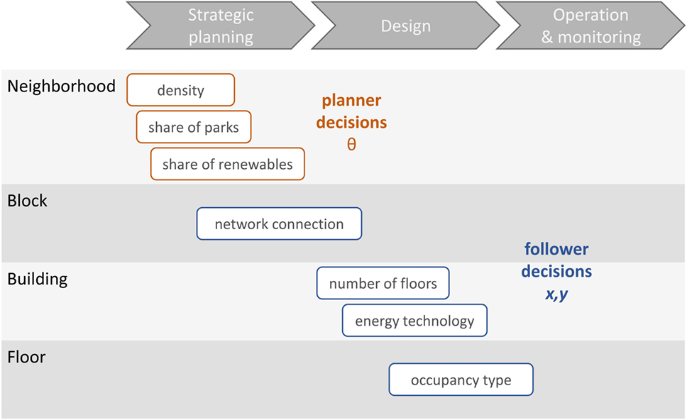
Figure 1. Examples of decisions to be made by different actors during the phases of an urban planning process and being implemented on different scales.

1.1. Choice of Methodology

The issue of a decision space too large to capture by a human leads to the employment of computation methods (Bruno et al., 2011; Saleh and Al-Hagla, 2012). One method of letting the computer not only evaluate scenarios, where all input is decided by humans, but also take decisions, is the application of optimization algorithms. Several classes of optimization algorithms exist, which differ by, e.g., speed, robustness against numeric starting conditions, permissible mathematical formulations, or if finding the global optimum is guaranteed (Reeves, 1993; Floudas, 1995; Bierlaire, 2015). Mixed-integer linear programming (MILP) is deemed to be especially suited for the purpose of this work, since it allows to comparably quickly generate a multitude of plans (Williams, 2013), and to include both continuous and discrete decision variables, but is easier to solve than mixed-integer non-linear programs (Conejo et al., 2006, p. 12). It lies in the nature of optimization that it leads to extreme solutions at corner points or edges of the solution space (Keirstead and Shah, 2013). This is, however, to some extent contradictory to the task of urban planners who rather have to balance many interests, which moreover are not even all quantifiable (Ligmann-Zielinska et al., 2008). Thus, the final outcome of the planning process might not lie on an extreme point of the solution space, which means that a mathematical optimum could be, but is not necessarily the goal (Brill, 1979; Markl et al., 2009; Bruno et al., 2011).

This insight is respected by the choice of different techniques for different types of decisions. The decision space is separated by sorting the decisions according to the actors who typically take them. The computer takes the multitude of the decisions of the followers while the human takes the typical planning decisions (Figure 1). A form of optimization that is suited for this purpose is known as multiparametric optimization where a number of decision variables are decided by the algorithm dependent on parametrized constraints (Gal, 1995; Pistikopoulos et al., 2007; Liu et al., 2011). A sampling technique is then used to systematically capture the decision space (Saleh and Al-Hagla, 2012) with all its bounds and interior tipping points (Scheffer et al., 2012) at which the system design would change subject to the decision of planners.

1.2. Research Goal

In this context, the research goal is to develop a multiparametric mixed-integer linear programming model that incorporates decisions for multiple domains, scales, phases, and actors of an urban development project. This article contains the description and demonstration of the optimization method and the developed model. Both form the computational basis for a decision support tool named URB^io, which was introduced in Cajot et al. (2017), and whose decision support aspects will be described in a future article. First applications of URB^io can be found in Cajot et al. (2016) and Hsieh et al. (2017).

Beforehand, existing literature on computer models is presented, which combine different domains and scales of urban planning, and which preferably employ optimization techniques.

1.3. State-of-the-Art

Batty (2009) sorts models in the urban field into three main classes: land-use transport (LUT) models, urban dynamics models, and models that represent individual agents as cellular automata, agent-based models, and microsimulation. Models of the first class (LUT) typically focus on the relationship between urban form and function as stated by Keirstead and Shah (2013). They also review LUT models that include optimization techniques. Examples for such models are the ones of Ligmann-Zielinska et al. (2008) and Kumar et al. (2016), who both use MILP to generate land-use plans on a city scale considering, e.g., the compatibility of adjacent land uses.

The work of Bruno et al. (2011) couples a parametric design software with a genetic algorithm to generate a multitude of urban plans and thus explore the decision space of urban planners heuristically. Their model comprises 5 decision variables for location, program, density, proximity, and mixed-use quality. Saleh and Al-Hagla (2012) make use of parametric design without employing an optimization algorithm to explore the interactions between urban form and environmental aspects, namely, the microclimate. Shi et al. (2017) have recently reviewed the efforts of coupling design generation software, with energy simulation and heuristic optimization algorithms to create and evaluate urban designs under energy aspects. Haque and Asami (2014) take heuristic optimization for urban planning down to the floor scale by including building height and mixed use via a continuous decision variable. They further consider different actors in form of governmental planner and land developer. The group “Kaisersrot” developed different computational tools for architectural or urban design from sub-floor to district scale employing statistical methods, concepts of self-organization, or optimization in form of genetic algorithms (Hovestadt, 2010). The examples they provide incorporate in different combinations urban form and function, social aspects as densities, proximities and view, and economic aspects as construction costs.

The so far mentioned articles have in common that energy aspects of urban systems are marginal, or completely out of their scope. On the contrary, however, there exists a whole body of research on energy planning. Relevant reviews include the ones by Mirakyan and De Guio (2013) and Huang et al. (2015), who compare tools that can be employed during different phases of the process of planning community or city-scale energy systems. Markovic et al. (2011) reviewed this kind of tools with an additional focus on the environmental impact of those energy systems. Allegrini et al. (2015) performed a review on computational methods that address the planning, design, and operation of energy supply systems spanning from building to district scale. One of the conclusions drawn is that there were still no tools that can be used for parametric analysis on the urban scale and that conform to an optimization process. The review of Reinhart and Cerezo Davila (2016) addresses the so-called urban energy building models (UBEM) designed for operational energy demand estimation. The listed works have as common goal the application of physically detailed building models on a neighborhood or city scale.

An overview over recent developments and applications of multiparametric programming is given by Oberdieck et al. (2016). Of the reviewed studies, the ones dealing with problems of bilevel programming and multiobjective optimization are closest to the purpose of this work. However, none is addressing the problem of urban or energy planning.

The ensemble of aforementioned reviews reveals that there are only few tools that consider both energy and non-energy aspects for the planning of urban systems. Existing work in this direction is presented in greater detail in the following. Riera Pérez and Rey (2013) use the decision support tool SméO to evaluate 3 urban renewal scenarios. Their work regards a quite complete range of urban planning aspects and spans the building to neighborhood scale. Robinson et al. (2007) developed SUNtool for fast and physically rigorous analyses of interdependencies between urban form and building energy demand. This is achieved by incorporating dynamic models, with a specific focus on shortwave irradiation exchange and user behavior. The tool was demonstrated on a case study of 100 buildings with each two thermal zones, thus spanning floor to neighborhood scales. Optimization is achieved by parametric studies although a coupling with, e.g., genetic algorithms was mentioned as a potential extension. Fonseca et al. (2017) use their tool CEA to examine the interactions between mixture of buildings’ occupancy types, environmental performance in terms of emissions and noise pollution, and resilience of both energy and transport infrastructure. They cover sub-building scales with, e.g., the calculation of user densities up to the scale of a new neighborhood of 25 ha. As for most previous tools, the urban form and function are user input in form of different design scenarios.

Following tools employ also optimization methods: Keirstead et al. (2009) introduced SynCity an integrated modeling framework for the design of minimum energy layouts in early-phase urban planning. This was especially achieved by introducing modeling of energy demand and supply into the field of optimization-based land-use models. To allow for a finer spatial resolution without significantly increasing computational costs they chose to use MILP (Keirstead and Shah, 2011). The case studies presented in Keirstead and Shah (2011) deal with the partly quantitative allocation of urban functions within a real district which is separated into about 40 distinct sites and a hypothetic, regular grid of 100 16-ha cells. Since the decision variables are surfaces and densities, the scale range should be rather classified as block to neighborhood, thus neglecting phenomena on building or even floor scale. Both the sizing of energy utilities and networks and the consideration of costs and partly even environmental implications in the form of emissions were included in SynCity for hypothetic grids of 16–256 cells (Keirstead et al., 2012) and in the tool DESDOP of Weber et al. (2010) and Weber and Shah (2011). However, both works considered the design of the energy supply utilities as a sequential step after the allocation and sizing of urban functions.

As a further development of the above presented SUNtool of Robinson et al. (2007) can be seen the tool CitySim (Kämpf, 2009; Robinson et al., 2009). In Kämpf et al. (2010), it is coupled with an evolutionary algorithm to optimize the design of a set of about 32 buildings with different, predefined block layouts in terms of their volume for their received annual irradiation offset by their thermal losses. Taking into account also the surroundings of the buildings their spatial scales span the buildings up to the district. The study focuses on the trade-off between urban form and solar potential. UMI is a Rhinoceros plug-in for the design of new neighborhoods (Reinhart et al., 2013). It incorporates social, energy, and environmental aspects. The urban form for each scenario has to be specified by the user and is thus extrinsic to the model. Presented case studies range from floor to neighborhood scale. Parametric modeling and optimization can be achieved using Grasshopper (Rakha and Reinhart, 2011). Best et al. (2015) developed a model for early-stage urban planning considering densities and building functions, which allows to simultaneously optimize energy supply and demand on an hourly time scale using a genetic algorithm. The smallest covered scale comprises floors. A larger scale is represented via an aggregation of individually simulated buildings.

1.4. Identified Gaps

The recent years have seen some progress toward a combination of several domains and scales within single tools. However, there still remain gaps, especially between the rather traditional urban planning domains concerning social aspects and urban form and function, and the energy planning domain concerning supply, transport, and demand of energy as well as its environmental and economic implications. This manifests in criteria of the, respectively, other domains either not being regarded or having to be provided as inputs to the model. Furthermore, tools that come from the field of building simulation often aim to take detailed modeling to larger scales. As these tools need relatively precise information regarding urban form, they tend to focus on urban design aspects rather than urban planning aspects (Reinhart et al., 2013). A second gap lies in the form of employed optimization algorithm if any. Almost all of the recently developed tools rely on heuristic optimization methods (Kumar et al., 2016). The last gap concerns the usage of multiparametric optimization: Despite the fact that it seems well suited, it was so far not applied to urban planning problems.

2. Methods and Material

2.1. Multiparametric Programming

This section shows how the task of urban planning can be stated as a multiparametric programming problem. Decisions are usually taken based on performance indicators Π, which are themselves a function of the former:

$\mathrm{\Pi }=F\left(\mathrm{\varphi }\right),\varphi \in \mathbf{\Phi },$ (1)

where ϕ denotes all variables whose values are to be decided (i.e., decision variables) within their regarding variable space Φ. Based on the recognition that the number of decisions is very large, further that these decisions are made by different actors at different phases of the urban development project, and last that all these decisions influence the final values of the performance indicators (see section 1), the decisions are roughly separated into decision variables θ, which are typically decided by planners at early phases and larger scales of the urban project, and decision variables x and y, which are typically decided by different stakeholders at later phases and smaller scales.

$\mathrm{\Pi }=f\left(\theta ,\mathit{x},\mathit{y}\right),\theta \in \mathrm{\Theta },\mathit{x}\in \mathbb{\text{R}},\mathit{y}\in \mathbb{\text{Z}}.$ (2)

Here, x denotes continuous variables and y denotes discrete (i.e., binary or integer) variables. They are decided by an optimization algorithm which solves the following multiparametric mixed-integer linear programming problem (Pistikopoulos et al., 2007):

$\begin{array}{lll}\hfill {\displaystyle \underset{x,y}{\text{min}}}& & f\left(\theta ,\mathit{x},\mathit{y}\right)=c_x^T\left(\theta \right)\cdot \mathit{x}+c_y^T\left(\theta \right)\cdot \mathit{y},\hfill \\ \hfill \text{subject to}& & P_x\left(\theta \right)\cdot \mathit{x}+P_y\left(\theta \right)\cdot \mathit{y}=p\left(\theta \right),\hfill \\ \hfill & & Q_x\left(\theta \right)\cdot \mathit{x}+Q_y\left(\theta \right)\cdot \mathit{y}\le q\left(\theta \right),\hfill \\ \hfill & & \theta \in \mathrm{\Theta },x\in {\mathbb{R}}_{\ge 0}^n,y\in {\mathbb{Z}}^q,\hfill \end{array}$ (3)

where optimal values for x and y are determined in dependence on the values of θ. x and y can thus be interpreted as rational reactions of the followers to the decisions of the planners θ (Pistikopoulos et al., 2007, p. 129f). In this work, the problem of the followers [equation (3)] is solved using a mixed-integer linear programming algorithm, while the problem of the planners [equation (2)] is explored via systematic sampling (Thompson, 2012) of the decision space. This means that the values of decisions of the planners θ are systematically changed, and the resulting values for decision variables of the followers x and y as well as the values of the performance indicators Π are captured.

2.2. Optimization Model

Criteria of the following domains are modeled: (a) urban form and function, (b) social aspects, (c) energy supply, distribution, and demand, and both (d) environmental and (e) economic implications.

The range of considered scales is set to cover the floor scale up to the neighborhood scale. The choice for the smallest scale is mainly due to the planning task of designing both horizontally and vertically mixed-use developments that foster social equality (Ligmann-Zielinska et al., 2005). The largest scale is selected to cover most of phenomena that only arise when looking beyond the building scale, while remaining small enough that actual outcomes of the model can have a practical meaning (Riera Pérez and Rey, 2013).

The model builds on common optimization modeling approaches for urban planning and the design and operation of energy systems, respectively. Where the model employs these approaches, only a short explanation of the equations listed in Tables 1–2 and references for further reading is provided. However, for some aspects the reviewed modeling approaches were found insufficient. After stating reasons for novel developments, those parts of the model are described in greater detail.

TABLE 1

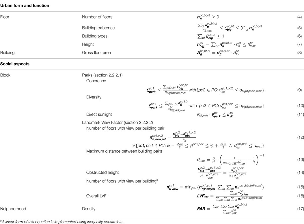
Table 1. Model equations for urban form and function and social aspects.

TABLE 2

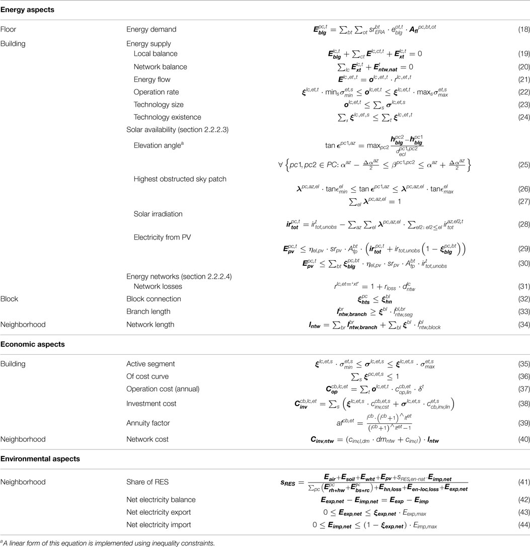
Table 2. Model equations for energy, economic, and environmental aspects.

2.2.1. General Overview

A planning site for a new neighborhood is divided into parcels on which buildings can be placed. These buildings are comprised of floors of potentially different occupancy types [equation (4)]. The buildings again can be of different types (e.g., mixed use or single family homes) and have type-dependent height limitations and typical footprints [equations (5)–(7)] (Haque and Asami, 2014). Based on the resulting gross floor area (GFA) [equation (8)] the density in form of floor area ratio (FAR) [equation (17)] can be calculated.

Further is this area used to estimate energy demands [equation (18)] (Keirstead and Shah, 2011) based on national norms for newly constructed buildings (see section 2.3.3.1). These demands have to be met by decentralized or centralized energy conversion technologies, where the latter are connected with the buildings via exchange technologies and networks. Closing the according energy balances allows to determine operation rates of each technology [equations (19)–(22)] (Samsatli and Jennings, 2013). These are used to calculate operation costs [equation (37)] and to determine the purchased technologies and their sizes [equations (23) and (24)] (Weber, 2008). Thus, the model accounts for both the design and operation of energy technologies. Using piecewise linearization to account for economies of scale, the active segment of the investment cost curves is selected with equations (35) and (36). These allow to calculate investment costs [equation (38)], which can be annualized with equation (39) (Yokoyama et al., 2002).

The share of renewable energy sources serves as an indicator to assess the sustainability of the energy supply. To calculate this share, the sum of all energy coming from such sources (air, soil, PV, waste heat, and partly the national electricity network) is divided by the sum of buildings’ demands, transport losses, and electricity exports [equation (41)].

2.2.2. Novel Model Components

2.2.2.1. Parks

Several authors covered the optimal allocation of parks on the city scale considering aspects such as population density, air and water quality, noise, the urban heat island effect, or land-use patterns (Neema and Ohgai, 2010, 2013; Yuan et al., 2011; Fernández et al., 2015). Assessments on the district to neighborhood scale treat, for example, the accessibility, connectivity, costs, number of beneficiaries, or population density, respectively (Sefair et al., 2012; Yu et al., 2014). This work focuses on the relationships between parks and their surroundings on the building to floor scale. The modeled aspects are inspired by the work of Jacobs (1961), who describes several basic principles characterizing parks with a positive contribution to their environment.

2.2.2.1.1. Coherence. First, parks should be enclosed and clearly delimited by a certain number of buildings, rather than isolated at the border of the community. Not only does a proper enclosure by buildings visually and spatially define the park as a positive feature but it also increases its accessibility. This is implemented by providing a constraint on occupied parcels around parks [equation (9)]. Implications of this constraint can be influenced by setting the minimum number of buildings around a park n_blg@park,min: Higher numbers result to more enclosed parks. Setting the maximum Euclidean distance between the park’s parcel and surrounding parcels d_{blg@parks,max} defines the perimeter in which surrounding buildings should be considered. Different combinations of both parameters allow to either enforce or prohibit specific layouts such as parks located at corners of blocks.

2.2.2.1.2. Diversity. Second, and related to the enclosure principle, surrounding buildings should offer a high diversity of uses. This in turns ensures a high diversity of users, leading to a more continuous occupation of the park throughout the day. In the model, this can be enforced by putting thresholds on numbers of floors of a certain occupancy type on parcels around parks [equation (10)].

2.2.2.1.3. Direct Sunlight. Third, the attractiveness of the park is also influenced by the amount of direct sunlight. Depending on the climatic context, complete obstruction of sunlight by tall buildings should be fostered or avoided. Here constraint (11) ensures a minimum of direct solar irradiation ir_dir (see section 2.2.2.3).

2.2.2.2. Landmark View Factor

The quality of living space and with it its cost is influenced by the view it offers on surrounding landmarks (Benson et al., 1998; Thalmann, 2010). In recognition of the demand for computer tools that inform planners, architects, and building contractors, previous attempts exist to visualize or quantify this view in computer models. The Ladybug plug-in for Grasshopper developed by Roudsari et al. (2013a) allows to visualize the obstruction to views from specified locations within a given urban scene by means of view roses. Ferreira et al. (2015) calculate the visibility of landmarks by rendering urban scenes from sampling points distributed over the landmark and determining buildings from which these points could be seen. Both of these tools estimate the view on a building scale without indicating a quantification on a neighborhood scale. In addition, they are designed to analyze extrinsically defined scenes where the here proposed model considers urban form intrinsically.

Consequently, a performance indicator to assess view quality is introduced here: The landmark view factor (LVF) is defined as the share of floors, either per building or per neighborhood, that have a view on a specified landmark. The number of floors per building with a view can be approximated by calculating the vertical part of a building from which the landmark could be seen and dividing it by the average floor height (see Figure 2A). This number is calculated for each pair of buildings, where one is potentially obstructing the view of the other [equation (12)]. This is accounted for by regarding only parcels that are both within a maximum distance d_max [equation (13)] and a certain, predefined angular range Δψ (see Figure 2B). This view range depends on the type of landmark. In the case of a natural land mark such as a mountain range, most likely only a broader view range would be considered as providing a building with a nice view than it would be the case with, e.g., an architectural landmark.

FIGURE 2

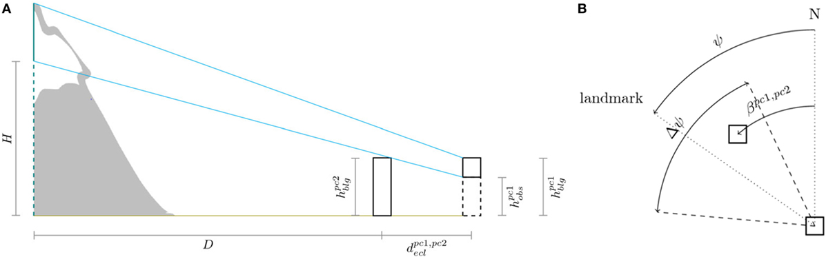
Figure 2. Views of a planning site to illustrate considered heights, distances and angles for the calculation of the LVF. (A) Side view. (B) Top view.

The height of the obstructed part of the building can be deduced from the height of the landmark H, the distance toward the landmark D and the Euclidean distance between the two considered buildings d_ecl using the intercept theorem [equation (14)]. In the case, there is no obstruction by any building the number of floors with a nice view equals the number of residential and office floors of the building [equation (15)]. Commercial floors are thus not being valorized for a nice view. To be able to compare resulting neighborhood layouts, an overall LVF is calculated [equation (16)].

2.2.2.3. Solar Availability

To assess solar availability, a novel method was developed that integrates cumulative skies into an MILP formulation. The electricity generated by PV panels depends on the tilt angle and area of these panels and on the amount of incident irradiation. The amount of solar irradiation during a specific time period coming from a specific sky patch can be assessed using cumulative skies (Robinson and Stone, 2004). The incident irradiation on the rooftop then depends on obstructions toward the sky vault. In urban surroundings, near-field obstructions depend mainly on the location and height of surrounding buildings. Therefore, for each azimuth direction of all sky patches, the maximum elevation angle of all rooftops is computed, that potentially obstruct sky patches in this direction [equation (25)] (compare Figures 3 and 2B). Using special ordered sets of type 1 (Beale and Tomlin, 1969) for the discretization of the sky vault, the highest obstructed sky patch is then determined according to equations (26) and (27).

FIGURE 3

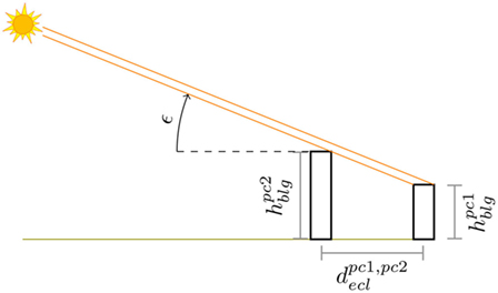
Figure 3. Calculation of obstruction to sun patch.

The surface-specific irradiation for each parcel and each time step is then a function of obstructed sky patches [equation (28)]. Finally, the upper bound for the electricity output of a roof mounted PV panel with electric efficiency η_el is resulting from equations (29) and (30) where the panel surface depends on the constructed building’s footprint and the share of roof surface available and suited for PV panel installation sr_PV.

2.2.2.4. Energy Networks

The network model was developed with the goal of obtaining a good estimation of the network lengths while increasing the problem size as little as possible. A conventional way to include the network layout in MILP formulations is to decide the existence of connections between nodes using binary variables for each potential connection (Söderman and Pettersson, 2006; Weber, 2008; Fazlollahi, 2014). For larger problems, this results into a high amount of binaries. In contrary, the method proposed here uses binary variables for the decision of whether a block is connected to a network. In principle, the method could be extended down to the building scale but currently a building can only be connected if a block is connected [equation (32)]. The network length and layout is then calculated based on branches and constraints on their lengths. For this purpose, potential network layouts for a planning site are identified. These layouts are then analyzed to identify branches: The main branch is starting at the point where the neighborhood scale network is connected to a heating center or a city-wide network. Following this branch, at each bifurcation it is checked for each bifurcating pipe if it connects more than one block. If so, an additional branch is defined. Otherwise, it is defined as a block connection whose length is stored. Afterward, it is determined for each pair of blocks and branches, how long the branch would at least have to be if the block was connected, resulting in the lengths of the branch segments. Each branch length is then calculated via equation (33), and the total length of a network is calculated via equation (34). From this, investment costs can be estimated [equation (40)].

Furthermore, distances between locations of supply and demand influence operation costs. An exchange technology extracts from the neighborhood-wide network [equation (20)], the amount required for satisfying the local balance [equation (19)] plus an amount to account for transfer losses [equation (31)]. Depending on the energy carrier, this loss is assumed proportional to both the amount of transferred energy and the distance over which the energy is transferred. This distance is calculated as the sum of the network distance and the Manhattan distance (Black, 2006) between the parcel and the point the block is connected to the network.

2.2.3. Relation between Model and Multiparametric Formulation

This section is concluded by indicating the roles of the presented variables and parameters in formulation (3): Discrete decision variables y for the optimization model are the number of floors of buildings n_fl [equation (4)], the existence ξ of buildings [equations (6)–(5)], parks [equations (9)–(11)], and energy conversion technologies [equations (29) and (30)] at specific locations, and the connection of blocks [equation (32)]. In addition, auxiliary variables are required for piecewise linearized functions as, e.g., λ for the sky dome model [equations (26)–(28)]. Core continuous decision variables x are the operation rates of technologies [equations (21) and (22)].

Although the planner could in principle adjust the values of all parameters, the main parameters are those that parametrize constraints by specifying minimum or maximum accepted bounds for performance indicators. The formulation of these constraints depends on the problem at hand, which will be illustrated in section 3.

2.3. Data

The case study, based on which the model was developed, is an ongoing greenfield development project aimed at transforming a rural zone into a neighborhood named Les Cherpines. This zone is located in the south-eastern part of the canton of Geneva, Switzerland. The development area comprises 58 ha and shall host 3,000 dwellings and 2,500 jobs. A neighborhood master plan has been issued in 2013 and defines several goals for the new development (Office de l’urbanisme, 2013). To cope with the increasing demand for residential and office space in the canton (Office de l’urbanisme, 2011), it shall achieve a high FAR. The new development shall meet “eco-district” standards corresponding to a coverage of at least 75% of the energy demand from renewable sources and the construction of buildings according to the Swiss energy label MINERGIE. Envisaged energy sources are among others low-temperature waste heat from an industrial zone located in the south-east of Les Cherpines, geothermal heat, and electricity from PV.

The spatial allocation of buildings is performed based on a preliminary site layout which is defined by the master plan (Office de l’urbanisme, 2013). It indicates the foreseen locations of major streets and some specific functionalities as an industrial zone in the southwestern part and a sports ground in the northern part of the area. To limit the initial scope of this study, the aforementioned elements were taken as fixed so that the remaining elements (i.e., buildings for residential and commercial purposes and for offices) are to be determined by the optimization. Based on the layout of the master plan a map is generated (see Figure 4) showing the various elements considered by the optimization model.

FIGURE 4

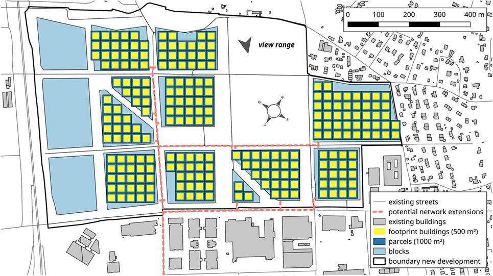
Figure 4. Map of the case study Les Cherpines.

2.3.1. Urban Form and Function

Statistical analyses of the building stock of Geneva were carried out using data provided by SITG (1957), to identify representative values for parcel and building parameters. The results are summarized in Table 3.

TABLE 3

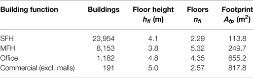
Table 3. Average values for form-related building parameters of the building stock of Geneva, for which the full set of listed parameters is available.

The permissible building height in the canton of Geneva is 21 m (Le grand conseil de la république et canton de Genève, 1988), which can be increased to 27 m to allow for an extra floor, if this floor is used for residential purposes. Thus, the maximum number of floors was set to 6.

The areas between the streets, which are already sketched in the preliminary layout (Figure 4), are defined as blocks and all blocks not containing any predefined building functions were meshed with a regular grid of evenly sized parcels. As a first approximation these parcels are taken to be quadratic. The parcels’ alignment deviates about 32.1° from global north toward west.

Based on Table 3, the footprint of mixed-use buildings and SFH is assumed to be 250 and 125 m², respectively. Afterward, the parcel size was set to 1,000 m² where each parcel is foreseen to host two buildings of the same type. These both decisions were taken out of several considerations: First, is this about the smallest size of existing adjacent parcels, which lie in the northeast of the new development (Figure 4), and allows thus a continuous urban form. Second, both decisions reflect the targeted trade-off between spatial detail and computational tractability since one building per parcel would mean doubling the number of parcels. Third, this parcel size allows to extend the model by the definition of typical office or commercial buildings which still would fit into a parcel each. And fourthly, the resulting building area ratio of one parcel is for mixed-use buildings 0.5 and for SFH 0.25, which is in line with common values for central and rural developments, respectively (Ruzicka-Rossier, 2005). The chosen parcel size resulted in a separation of the case study area into 233 parcels.

2.3.2. Social

Table 4 lists assumed surface values related to residential use. An average gross floor area per job of A_jobs = 30 m² was taken from Rey and Lufkin (2013).

TABLE 4

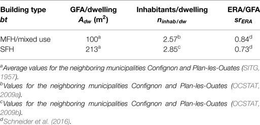
Table 4. Dwelling surface, occupancy rate, and surface ratio for two building types (GFA, gross floor area; ERA, energetic reference area).

2.3.2.1. Landmark View Factor

A mountain range named “Jura” can be seen from the area, which peaks at about 1,700 m. Table 5 lists the parameters required for calculating the LVF under the assumptions that one wants to see at least the uppermost 300 m of altitude.

TABLE 5

Table 5. Geometric parameters for calculating the landmark view factor.

2.3.3. Energy

2.3.3.1. Energy Demand

The project goals require that all buildings should be constructed according to the Swiss MINERGIE-P standard for thermal insulation of buildings. This standard defines a peak heating demand of 10 W/m² for all buildings (MINERGIE, 2016), which is here also assumed for peak cooling demand. The annual energy demands listed in Table 6 are based on the Swiss SIA directive for energy efficient buildings and include auxiliary energy for heating systems, ventilation, electric appliances, and lighting.

TABLE 6

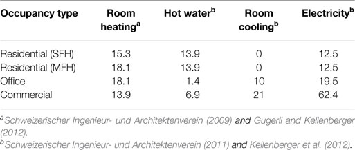
Table 6. Energy reference area-specific annual energy demands per occupancy type (kWh/m² a).

Supply temperatures of 12°C for cooling requirements and 55°C for hot water and heating requirements (Girardin, 2012, p. 78) were assumed to estimate coefficients of performance of chillers and heat pumps, respectively.

2.3.3.2. Energy Supply

For this study, only centralized CHP technologies are foreseen, while chillers and PV panels are installed only at the buildings. Boilers and heat pumps can be installed both centrally or decentrally. Two different annual efficiencies are used for heat pumps to account for higher efficiencies of larger, centralized technologies. Table 7 lists the different efficiencies for all considered energy conversion technologies.

TABLE 7

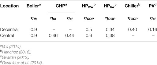
Table 7. Efficiencies of energy conversion technologies.

The numerical assumptions regarding the estimation of PV potential include the panels’ conversion efficiency (see Table 7), the available roof surface area for PV panels, the panels’ tilt angle, and the skydome. The roof surface can be partly shaded by roof superstructures such as chimneys or machine rooms for elevator systems. Furthermore, the roof surface available for PV panels might be reduced by windows. After reduction of these factors the remaining surface is still not equal to the collector surface since in the case of flat roofs the panels should be mounted with a certain tilt angle to maximize the incident annual irradiation on the panels, depending on the geographical location. Consequently, it is assumed here that the PV panel area is 50% of the footprint area. In addition, a panel tilt angle of 30° is taken (Desthieux et al., 2014, p. 19), which maximizes the annual solar irradiation exploitation for the latitude of Geneva.

In principle, a skydome containing the 145 sky patches of the Tregenza sky could be used to assess the solar potential. The piecewise linear formulation, however, requires a binary variable for each sky patch. Thus, the MILP problem would become already for small numbers of parcels quite large. This can be counteracted by disaggregating the sky vault into a smaller number of patches (Figure 5).

FIGURE 5

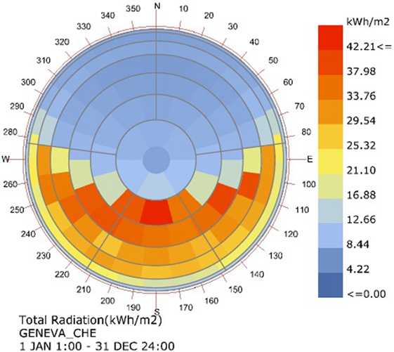
Figure 5. Top view of a spheric skydome indicating the total annual irradiation on a surface tilted 30° toward south for the location of Geneva: aggregation into larger patches indicated by gray lines (cumulative sky created with Ladybug; Roudsari et al., 2013b).

2.3.3.3. Energy Networks

Losses in the electric grid are assumed as 5% of the supplied electricity (Best et al., 2015, p. 164) while losses in the gas grid are neglected (Keirstead et al., 2012, Table 2). Losses in the heating network are estimated as 4.3% of supplied heat per kilometers of network distance (Keirstead et al., 2012, Table 2). Its nominal supply temperature is set to 60°C at the heating center.

An industrial zone is located toward the south-east of the area with already installed pipes for a heating network. Consequently, an attractive option could be to employ the incidental waste heat for satisfying the new neighborhood’s energy demands. The waste heat is taken as being constantly available over the year with a power of 10.75 MW at a temperature of 20°C.

2.3.4. Environment

Table 8 lists the meteorologic parameters that influence the design of the energy conversion technologies. The EnergyPlus weatherfile available for Geneva is used to generate the cumulative sky (EnergyPlus, 2017). Furthermore, a constant soil temperature of 10°C is assumed (Weber and Shah, 2011).

TABLE 8

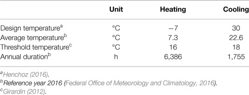
Table 8. Meteorologic parameters.

For the calculation of the RES shares on parcel and neighborhood scale, a RES share of 47.1% for the Swiss supplier electricity mix is taken, considering only electricity from verifiable sources and further taking waste incineration as renewable (Frischknecht et al., 2012).

2.3.5. Costs

Assumed interest rates are as follows: 1.7% for owner-occupants (reference year 2016) (Schweizerische Nationalbank, 2017) and 6% for the energy provider (OFEV, 2016).

2.3.5.1. Energy Supply

An economic lifetime of 15 years is taken for all energy conversion technologies (Henchoz, 2016, p. 82). For the economic analysis, cost functions of several authors were compared. Non-linear cost functions were linearized with up to 5 segments where the choice of number and range of segments was made to achieve a good approximation of the original function. The resulting ranges, intercepts, and slopes of these segments are listed in Table 9. A conversion factor of 1.1 CHF/EUR is used for the costs of Voll (2014) and Henchoz (2016).

TABLE 9

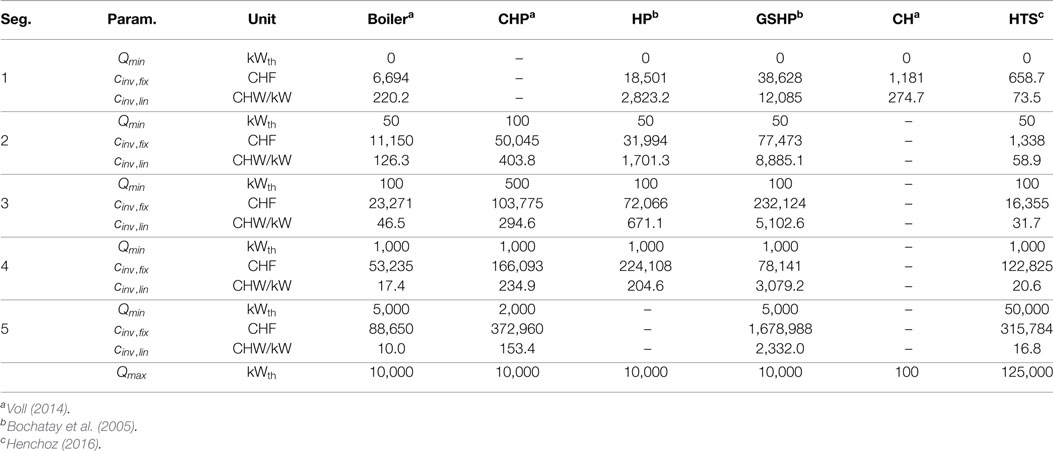
Table 9. Linearized cost functions of energy conversion technologies.

The same cost function is used for air–water heat pumps and water–water heat pumps, neglecting the additional costs of air–water heat pumps due to larger heat exchangers. The cost function for GSHP includes the costs for the geothermal probe. The cost function of Voll (2014) for CHP technologies is extrapolated below 0.5 and above 3.2 MW. To convert the reference quantity of the cost function for heat exchangers given by Henchoz (2016) from area to power, his assumed heat transfer coefficient of 2.5 kW/m² K and an estimated logarithmic mean temperature difference of 5 K were used. For PV panels, a fixed cost coefficient of 4,000 CHF/kW_peak is taken (Desthieux et al., 2014, p. 33).

2.3.5.2. Energy Networks

For the calculation of operation costs, an electricity price of 0.2076 CHF/kWh (Eidgenössische Elektrizitätskommission, 2016) is assumed for all actors. Further prices are listed in Table 10. The heat price at which the local supplier buys is the price for waste heat of the industrial zone and is an assumption of the authors.

TABLE 10

Table 10. Energy prices in CHF/kWh.

For the calculation of investment costs an economic lifetime of 40 years is taken. Consequently, repeated investments in conversion technologies with lifetimes shorter than 40 years (see section 2.3.5.1) are taken into account for the calculation of, e.g., the annual rate of return (Henchoz, 2016, p. 82). As the new development is located within the city boundaries, some infrastructure is already existent, e.g., electric lines which are passing by all blocks. Consequently, no installation costs for an electric grid are considered. The city-wide gas grid is assumed to end at the same point as the existing heating pipes confidentiality issue Figure 4. The investment costs for new gas pipes are estimated with a factor of 375 CHF/m based on Keirstead et al. (2012) (Table 2). To estimate the investment costs for a new heating network the cost function of Henchoz (2016) (Table 1.12) is used with a length- and diameter-specific cost factor of 5,670 CHF/m² and a length-specific cost factor of 613 CHF/m. An average diameter of the network pipes of 0.15 m is assumed based on existing networks in comparable neighborhoods. The resulting length-specific costs are in the range of the costs given by Keirstead et al. (2012) (Table 2).

3. Application

3.1. Influence of Density and Share of Renewables on Energy System, Costs, and Urban Form

The developed methodology is demonstrated by answering two practical questions. The first one is addressing a cost effective energy supply system: What are the implications of the decisions of the planners regarding density and environmental targets on the resulting energy supply system assuming that the owner-occupants of the buildings and the local energy supplier act according to economic interests?

The density target consists in the FAR that the new neighborhood should have, and the environmental target is the share of RES its energy supply shall achieve. These two indicators form thus the decisions of the planners θ in equation (2), and their values are varied systematically to capture the according decision space. The second group of actors affected by the given question is the owner-occupants of the buildings. They are assumed as one homogenous group that has the common and only goal of limiting their energy-related costs. Thus, the assumption is made that all buildings are occupied by their owners and no conflict of interest exists as might be the case for landlords and tenants. This means that annualized investment cost and annual operation cost for the energy supply are paid by the same actor. The third considered actor is the local energy supplier whose task is the provision of the energy infrastructure with networks and centralized technologies. Similar to the group of owner-occupants, it is assumed that the supplier follows an economic interest that might manifest itself in providing only supply options that guarantee them a certain annual rate of return. All numeric values are listed in section 2.3. The above listed interests translate into the following optimization problem:

$\begin{array}{ll}\hfill \text{min}& {\displaystyle \sum _{\mathit{pc}}}{\displaystyle \sum _{\mathit{et}}}\left({\mathit{af}}^{\mathit{cb}\text{=}\mathit{‘owner’,et}}\cdot {\mathit{C}}_{\mathit{\text{inv}}}^{\mathit{cb}\text{=}\mathit{‘owner’,pc,et}}+{\mathit{C}}_{\mathit{\text{op}}}^{\mathit{cb}\text{=}\mathit{‘owner’,pc,et}}\right),\hfill \\ \hfill \text{subject to}& {\mathit{FAR}}_{\mathit{min}}\le \mathit{\text{FAR}}\le {\mathit{FAR}}_{\mathit{max}}={\mathit{FAR}}_{\mathit{min}}+0.01,\hfill \\ \hfill & s_{\mathit{RES,min}}\le {\mathit{s}}_{\mathit{\text{RES}}},\hfill \\ \hfill & {\mathit{RR}}_{\mathit{min}}\le \frac{-{\mathit{C}}_{\mathit{\text{op}}}^{\mathit{cb}\text{=}\mathit{‘supplier’,et}}}{{\sum }_{\mathit{et}}{\mathit{C}}_{\mathit{\text{inv}}}^{\mathit{cb}\text{=}\mathit{‘supplier’,et}}+{\mathit{C}}_{\mathit{inv}\text{,}\mathit{ntw}}}.\hfill \end{array}$ (45)

3.1.1. Decision Space of Planners

Figure 6 shows the decision space of the planners that was captured by solving the above stated optimization problem. On the horizontal axes, the decision variables of the planners are plotted, one out of the social domain with the FAR, and the other out of the environmental domain with share of RES. Figure 6A displays performance indicators for owner-occupants out of the economic domain, with total costs on the vertical axis and operation costs on the color bar. Figure 6B shows indicators for the energy supply system in form of connection rates, which reflect the shares of buildings that are connected to the heating network (vertical axis) or the gas network (color bar), respectively. Figure 6C presents indicators for the urban form, with the building area ratio (BAR) on the vertical axis and the average building height on the color bar. Each point on the resulting surfaces is a single plan for which all decisions of the followers are fixed according to equation (45). Small circles indicate selected plans, for which the urban layout is given in Figure 7.

FIGURE 6

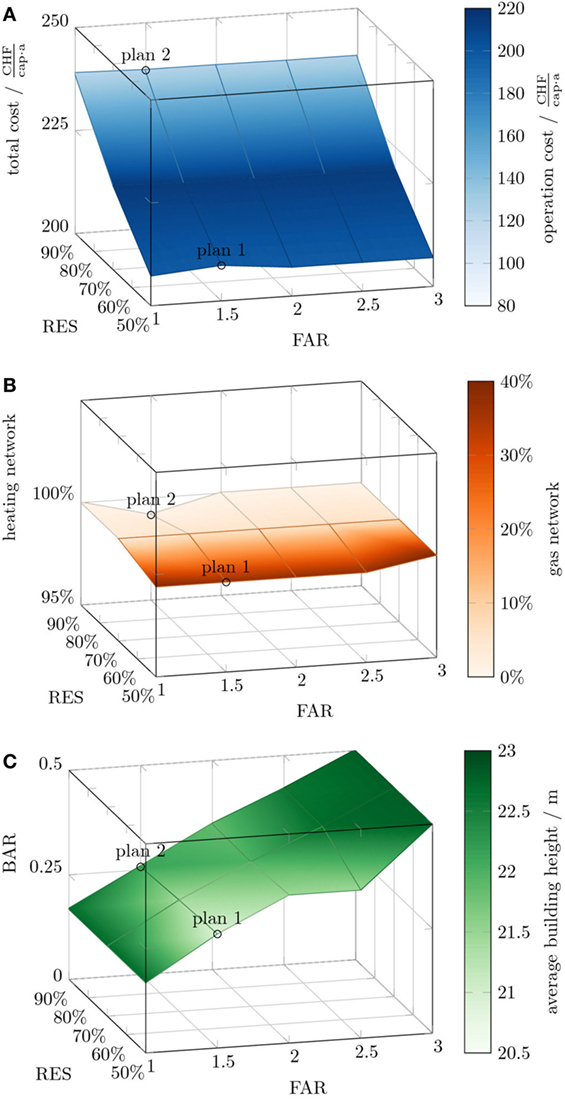
Figure 6. Capturing the decision space for planners: impact of their decisions on density and share of RES (horizontal axes) on 6 indicators (vertical axis, color bar) for costs, energy system, and urban form (circles indicate plans that are presented in more detail in section 3.1.2). (A) Costs of owner-occupants, (B) connection rates, and (C) urban form.

FIGURE 7

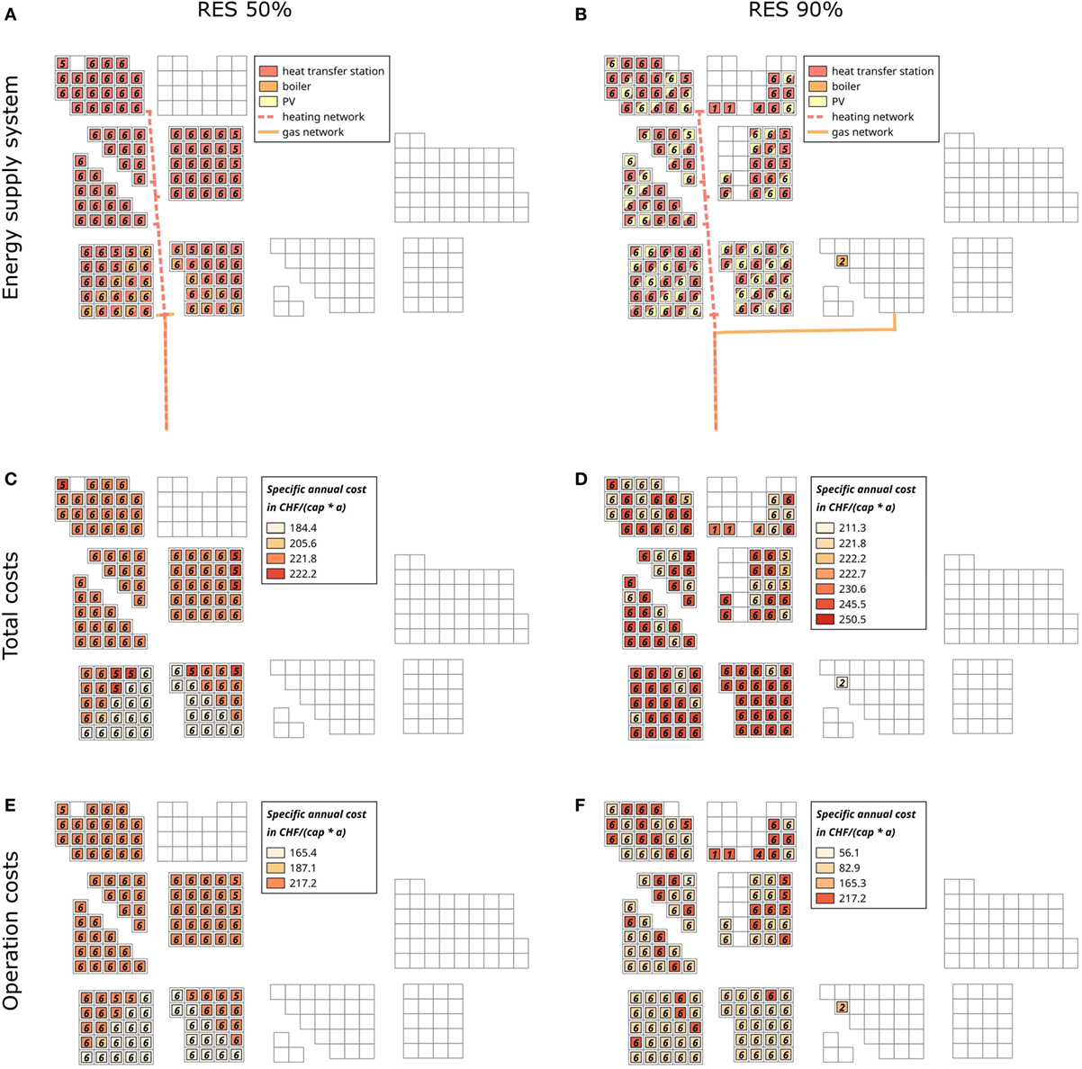
Figure 7. Urban form and energy supply system for selected plans of varying shares of RES and a constant FAR of 1.5 (numbers indicate total floors). (A) Plan 1 (RES 50%): energy supply system. (B) Plan 2 (RES 90%): energy supply system. (C) Plan 1 (RES 50%): total costs. (D) Plan 2 (RES 90%): total costs. (E) Plan 1 (RES 50%): operation costs. (F) Plan 2 (RES 90%): operation costs.

Figure 6A reveals that an increasing share of RES leads to an increase in capita-specific total costs of the owner-occupants, which form the objective function, but a decrease in their operation costs. This is due to the choice of owner-occupants regarding their energy supply system which will be illustrated in greater detail in section 3.1.2. It is further remarkable that an increasing FAR implies only a very small decrease in total costs.

The indicators for the energy supply system (Figure 6B) show that all buildings are connected to the heating network independent on the targets for FAR and share of RES. Furthermore, the gas network connection rate decreases with an increasing share of RES, which prevents natural gas as source for heating. A dependency of the connection rates on the FAR is not recognizable. The reason therefore will become clear when observing the effects on the urban form indicators: Figure 6C illustrates that the increase in FAR is achieved by increasing the BAR of the neighborhood rather than constructing taller buildings. First, it is less costly for the group of owner-occupants to install fewer energy technologies of larger size than many small technologies due to a sublinear increase of their investment costs with nominal power (see section 2.3.5.1). This also explains why almost no decrease of total costs of owner-occupants with an increasing FAR is detectable in Figure 6A. Second, small buildings that have to be spread out over more parcels to obtain a given FAR, require longer energy network connections than few, tall buildings. However, since all buildings are connected to at least one energy carrier network (see Figure 6A), the constraint on supplier costs demands for a grouping of this building into a few blocks, close to the feed-in point of the existing networks, to decrease the total network lengths and therewith investment costs.

3.1.2. Decisions of Followers

Two plans are presented in detail to exemplarily illustrate the decisions of the followers. Figure 7A shows that the buildings are clustered to assure the supplier the targeted annual profit as stated earlier. Furthermore, all buildings are connected to the heating network. In addition, about 40% of all buildings use natural gas boilers. All buildings connected to both networks import annually 2.1 GWh of natural gas and 30.4 MWh of heat. Thus, the heat received from the heating network covers only the peak load in cold hours. Figure 7C reveals that under the given prices this combination would indeed be cheapest for the owner-occupants. However, it is not employed in all buildings since the constraint on RES puts a limit on the usage of natural gas for heating. Although the chosen energy supply system respects the constraint on annual supplier profit, is it unlikely that a supplier would be ready to offer this option. To prevent these designs, the model and according data could incorporate, e.g., load-dependent heat prices, or an additional constraint to exclude connections to both networks.

In plan 2, again all buildings are connected to the heating network and clustered in 6 blocks (Figure 7B). However, the higher minimum share of RES of 90% allows only one building to be heated by a boiler yet. Furthermore, this constraint requires to equip about 35% of all buildings with PV panels. The installation of these panels means that the owner-occupants of those buildings pay higher total costs (Figure 7D), but lower operation costs (Figure 7F).

3.2. Influence of Density and Share of Parks on Landmark View and Urban Form

If followers acted purely economically driven, the previously identified plans would best reflect their interests. However, these plans are not attractive under other considerations since a densely clustered, high-rise environment is likely to not be considered very livable by most occupants. One implication of such dense plans is that open spaces are not nearby or even entirely missing (i.e., for an FAR of 3). A further implication is that the view on, e.g., surrounding landmarks is very limited. Such a view influences in turn the prices of buildings or flats within these buildings, at which building contractors can sell them to owner-occupants (Benson et al., 1998; Thalmann, 2010). Inspired by these shortcomings, a second practical question aims at aspects of livability rather than the energy system and its economic and environmental effects: what are the implications of the decisions of the planners regarding density and park targets on the resulting urban form assuming that the building contractors try to maximize the view of all buildings? The resulting optimization problem is given by:

$\begin{array}{ll}\hfill \text{max}& {\displaystyle \sum _{\mathit{pc}}}{\mathit{n}}_{\mathit{fl},\mathit{\text{view}}}^{\mathit{pc}},\hfill \\ \hfill \text{subject to}& {\mathit{FAR}}_{\mathit{min}}\le \mathit{\text{FAR}}\le {\mathit{FAR}}_{\mathit{max}}={\mathit{FAR}}_{\mathit{min}}+0.01,\hfill \\ & s_{\mathit{park,min}}\le \frac{{\sum }_{\mathit{pc}}{\mathit{\xi }}_{\mathit{\text{park}}}^{\mathit{pc}}\cdot A_{\mathit{par}}^{\mathit{pc}}}{{\sum }_{\mathit{pc}}{A}_{\mathit{par}}^{\mathit{pc}}}.\hfill \end{array}$ (46)

To respect the conditions for livable parks (section 2.2.2.1), it is assumed that parks are surrounded by at least 5 buildings [equation (9)], which together comprise a minimum of 3 residential floors, 2 office floors, and 1 commercial floor [equation (10)], and which are not further away than 50 m. Besides that, parks shall have a minimum annual solar irradiation of 500 kWh/m² a [equation (11)].

3.2.1. Decision Space of Planners

Figure 8 shows a similar plot as for the first question, which illustrates the decision space for planners. The surface spanning up this space is of triangular shape, which is due to the existence of a maximum achievable share of parks for a given density. It can be further noted that the achievable LVF increases with decreasing FAR and decreasing share of parks, respectively. Within the given ranges of FAR and park share, the FAR has the bigger effect on LVF. This observation will get clear when looking at the map indicating the decisions of all followers.

FIGURE 8

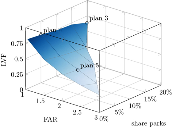
Figure 8. Capturing the decision space for planners: their decisions on density and share of parks influence the maximum achievable LVF (circles indicate plans that are presented in more detail in section 3.2.2).

3.2.2. Decisions of Followers

For a low density of 1 and a low park share of 5%, a very high LVF is obtainable: 78% of all floors have a nice view (Figure 9B). For most blocks, the highest buildings, and thus with best view, are located at the south-eastern-most row of parcels, the furthest away from the next block in the direction of the landmark. This has two implications: The highest buildings line up at the south-eastern border of the plan, perpendicular to the direction of a nice view. In addition, there is a diagonal line of high buildings. Almost all buildings located north of this diagonal have only one floor. The parks are mainly located at the north-western border of the blocks and unevenly distributed over the neighborhood. This could be counteracted by a constraint on the spatial distribution of parks.

FIGURE 9

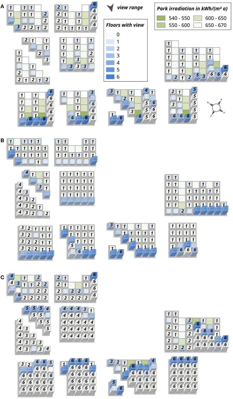
Figure 9. Urban form, landmark view, and park irradiation for selected plans of varying densities and park shares (numbers indicate total floors). (A) Plan 3: FAR 1.0, park share 20%. (B) Plan 4: FAR 1.0, park share 5%. (C) Plan 5: FAR 2.0, park share 5%.

For the same density but a higher park share of 20%, the achievable LVF is 64% (Figure 9A). The higher number of parks implies that less parcels can be occupied by buildings. To still achieve the same FAR, the floors have to be stacked up to less, but higher buildings. These few, high buildings are obstructing the view more than many, small buildings. The parks are arranged in the form of long “alleys” in the direction of the landmark. More shaded areas are located at the southern-eastern ends, surrounded by the higher buildings with nice views. Due to those alleys, many floors of these buildings, however, have rather a tunnel view on the landmark. An improvement of the concept of the LVF could thus include the visible range of the landmark. Furthermore, those alleys could be combined to form less numerous but therefore wider park alleys by increasing the perimeter d_{blg@parks,max}, within which surrounding buildings should be considered, for the constraints on coherence [equation (9)] and diversity [equation (10)]. Those alleys also bring about that especially from the south-eastern ends of the parks, the landmark is more visible. Thus, in comparison with the previous plan 4, a shift from private view toward public view can be stated.

For the same park share as for plan 4, but with a higher density of 2, at most 39% of all floors can have a nice view (Figure 9C). Rather than lines of high buildings, the algorithm generates blocks of mainly the same building height, where height differences mainly occur between blocks. Here, the first row of each block in view direction enjoys a nice view. Parks are located at almost the same parcels as for the case of a lower density.

4. Discussion

4.1. Key Contributions

Urban planning comprises many conflicting goals, which are not easily resolvable and whose solution is commonly left to the intuition of the planners. The presented approach takes up this practice by offering them a computational method where they can quickly detect the impact of their decisions on those the followers are likely to take. By aggregating the decisions of the followers to planning parameters, as densities or shares of, e.g., parcel functions, the method is targeting early planning phases. The combination of several domains in one model allows to simultaneously regard multiple aspects of urban planning, namely, social, economic, form, environmental, and energy aspects, which commonly have to be tackled with different tools.

The computational method employs optimization to assist in resolving conflicts between these domains. It aims to do so, not by calculating the ultimate solution, but aggregating the results of many optimizations to reveal potentials, limitations, trade-offs, and contradictions of and within the decision space of the planners. The application of the method to answer two practical planning questions revealed, e.g., the impact of sustainability targets on the energy supply system or the maximum achievable view factor in dependence on number of parks.

Results are in first line available in form of three-dimensional charts of the decision space, which reveal the general trends and trade-offs inherent to the planning question at hand. Maps showing the decisions of the followers serve to explain and understand in detail these observed trends and trade-offs rather than providing a final urban design. They may serve as basis from which planners continue based on their intuition and experience.

4.2. Limitations

4.2.1. Validity of Results

Model-based methodologies face the trade-off between detail and accuracy on the one hand and computational costs on the other hand. If such methods were ordered according to this trade-off, the one proposed would rather lie somewhere in the middle. It is more detailed but also more costly than spreadsheet tools, which serve to do rough estimations, but are limited when it comes to generating and optimizing a great number of plans. On the other hand, it is less detailed but also less costly than dynamic simulation tools, which serve to, e.g., create operation schedules, and which are mostly fit for specific purposes, such as the estimation of energy demand in buildings or transport needs. These kind of tools would further have to be coupled with heuristic optimization methods to reveal similar insights as the proposed tool is able to give.

The advantage in computational speed over the group of simulation tools is partly achieved by only allowing linear model formulations. They come at the price of modeling accuracy since many phenomena arising in the urban context are of non-linear nature. Although this can be partly overcome by piecewise linearization of non-linear functions, as also employed in this work, this remains an approximation.

However, since the task in early-phase urban planning is to create, compare, and decide between different sketches, users might be ready to accept a lower degree of accuracy for getting a better overview of their decision space in a faster way. A certain number of thus identified sketches could then be validated with more accurate and detailed simulation tools.

4.2.2. Interpretability of Results

Another limitation next to the accuracy of generated results is their interpretability. On the one hand, plans found by numerical optimization should first of all be considered as extreme solutions (Keirstead and Shah, 2013, p. 330f). Although there is the possibility to make the plans less extreme and more balanced by subsequently adding constraints respecting more and more aspects, their extreme nature will persist. It is therefore left to the planner to adequately make use of these extreme solutions and insights in a meaningful way (deVries et al., 2005).

On the other hand, interpreting the generated abstract urban form, depicted by a regular grid occupied with cubes, is not straightforward. This form should be interpreted as representing relationships (Bruno et al., 2011, p. 105) and would naturally not be built directly. So far the planner would still have to deduce the rules expressed by the arrangements of the blocks and translate them into a realistic urban form. A first step in such a process could be to move the buildings as placed by the algorithm within their parcels or to reshape their footprint while respecting the FAR, building height and floor types as calculated by the model. However, the greater these changes, the more likely it is that certain calculated indicators do not hold anymore. Thus, a validation with more detailed simulation tools would become even more important. One could also think of a new series of optimizations using different assumptions on size and position of footprints and parcels. In summary, the generated results, not only but especially concerning the urban form, should not be seen as dogmatic but indicative.

4.2.3. Balanced Modeling

A third limitation lies in the fact that not all aspects of urban systems are easy to quantify and thus to include in the model (Ligmann-Zielinska et al., 2008; Bruno et al., 2011). Williams (2013) states that the necessity to take decisions, however, often implies an implicit quantification of “unquantifiable concepts,” and that in comparison with such an implicit quantification, the endeavor to make a quantification explicit is preferable. The degree of ease with which criteria can be measured and modeled can even affect the attention they are given (Roy, 1985; Meadows, 1998; Desthieux, 2005). In this line, it would be imperative to include as many aspects as possible in the model, even though or yet especially if they seem very hard to quantify. Another approach would be to use the proposed methodology to identify a few plans that are promising concerning the modeled aspects and subsequently assess these plans regarding aspects that are not modeled. The arrangement of buildings, for example, illustrates well both philosophies: Design rules based on expert knowledge could possibly be identified, which could then be implemented in the model On the other hand, the generated maps allow—with a certain faculty of abstraction (see section 4.2.2)—an a posteriori judgment by a human (Bruno et al., 2011).

4.2.4. Graphical Representation

The decision space of planners was represented by plotting criteria on three spatial axes and coloring the resulting surface (Figures 6 and 8). However, these plots are naturally limited in the number of indicators presented at the same time, and make it hard to identify numeric values. A graphical representation to overcome these limitations is the use of parallel coordinate plots (Cajot et al., 2017).

4.3. Potential Future Work

4.3.1. Exploitation of Model

Potential future work could start with a further exploitation of the already existing model. For example, the two presented practical questions could be combined to one optimization problem to assess the trade-off between a clustering of high-rise buildings, which is desirable to reduce energy related costs (section 3.1), and a scattering of buildings of various heights, which increases livability (section 3.2). In addition to that, other insights could be gained by alterations of the underlying data, e.g., by varying the energy prices or considering different occupancy types.

4.3.2. Extension of Model

4.3.2.1. Scales

Although the model already spans a considerable range of scales from floor to neighborhood, there is still plenty of room to incorporate more spatial scales. This holds especially for enlarging the considered scales toward the district or even beyond. A first step in this direction was done with looking at nearby resources, here in form of waste heat from a neighboring industrial zone. However, there are other aspects and also other domains where an expansion of the focus should have an impact on decisions. An example therefore would be the optimization of the landmark view within the new neighborhood while compromising as little as possible the landmark views of existing, surrounding neighborhoods.

With just 4 time steps (base and peak demand of heating and cooling, respectively), the temporal resolution of both input data and results is very low. A refinement of the temporal scales by, e.g., incorporating typical days should allow to incorporate the effect of operation strategies on the system performance. An extension toward larger time scales is also conceivable to determine not only where and what kind of buildings or equipment to build or purchase, respectively, but also when.

4.3.2.2. Domains

Not only could further scales but also further aspects of urban systems be considered. The current model incorporates, for example, only operational energy demand. Further work could thus implement the embodied energy and greenhouse gas emissions due to the construction of buildings and the energy supply system. The underlying trade-offs between embodied and operational energy should indeed influence the decisions (Kellenberger et al., 2012, p. 86). Also would the primary energy demand for energy technologies allow to compare the performance of the neighborhood with target values as defined by the 2000-Watt society concept (Schweizerischer Ingenieur- und Architektenverein, 2011). Likewise non-energy related environmental aspects could be included as, e.g., soil permeability. A domain which was so far entirely left aside concerns the mobility of the neighborhood’s occupants.

4.3.2.3. Application

The model could be further adopted to also apply to redevelopment projects of existing neighborhoods where the outer form of only a part of the building stock might be subject to change. While this would reduce the relevance or necessity, respectively, of some indicators and decision variables, others might be more important or additionally required.

4.3.3. Extension of Methodology

4.3.3.1. Capturing the Decision Space

The goal of capturing the decision space and its tipping points can be achieved in computationally more efficient ways than proposed here. One way of doing so is to employ more sophisticated sampling techniques to determine the combination of parameters (i.e., decisions of planners) for which an optimization over the decisions of the followers shall be performed. Another way consists in the use of dedicated multiparametric programming algorithms to identify critical regions (Pistikopoulos et al., 2007; Kopanos and Pistikopoulos, 2014).

4.3.3.2. User Interaction

The answer to a specific planning question might result in the conjecture that there are more hidden trade-offs and thus bring up new questions. These new questions can be answered independently, as was done for this article, and could be considered as looking at the decision space from a different, independent perspective. However, this approach risks to result in conflicting plans and thus making decisions difficult again.

It would be better to answer newly arising questions building on the already obtained results, e.g., fixing the energy supply system identified in the first step and then optimizing the LVF. This constitutes rather a deeper exploration of the decision space. A third way would be to adapt the original problem statement with respect to newly discovered or suspected trade-offs. This requires in the following a recapturing of the decision space. Which of these approaches is suited, highly depends on the decision-maker and the questions at hand. Consequently, an interface would be needed to let the decision-maker steer the exploration of the decision space by defining and refining objectives and constraints. Based on discussions with different stakeholders of the urban domain, such an interface is currently under development to complete the decision support tool URB^io.

Nomenclature

α	Azimuth angle of sky patch
β	Angle from north toward direction of building
δ	Duration of time step
Δψ	View range around landmark
ε	Elevation angle of sky patch
λ	Binary variable for sky patch
ϕ	All decision variables
Π	Performance indicator
ψ	Angle from north toward direction of landmark
σ	Reference size of technology
θ	Decision variables for user, parameters for model
ξ	Existence of …
A	Area
af	Annuity factor
C	Cost
c	Vector containing objective function coefficients
D	Distance to landmark
d	Distance
dm	Diameter
E	Energy flow
e	Specific energy flow (to area or length)
H	Height of landmark
h	Height
hn	Heating network
hts	Heat transfer station
i	interest rate
ir	Surface-specific irradiation
l	Length
lt	Lifetime
n	Number of …
o	Operation rate of technology
P	Matrix containing equality constraint coefficients
p	Vector containing right-hand side parameters of equality constraints
Q	Matrix containing inequality constraint coefficients
q	Vector containing right-hand side parameters of inequality constraints
r	rate-specific energy flow
RR	Rate of return
s	Share
x	Continuous decision variables for computer/optimization
y	Continuous decision variables for computer/optimization
Acronyms
ASHP	Air source heat pump
CH	Chiller
CHP	Combined heat and power
ERA	Energetic reference area
FAR	Floor area ratio
GFA	Ground floor area
GSHP	Ground source heat pump
HP	Heat pump
HTS	Heat transfer station
LVF	Landmark view factor
MFH	Multifamily home
MILP	Mixed integer linear programming
PV	Photovoltaic
RES	Renewable energy sources
Set members
com	Commercial
mix	Mixed-use building
off	Office
rsd	Residential
sfh	Single family home
Subscripts
air	Heat from the air
blg	Building
bs	Building services
cst	Constant part of equation
dir	Direct
dm	Diameter specific
ecl	Euclidean
en-loc	Local electricity network
en-nat	National electricity network
exp	Export
fl	Floors
fp	Footprint
gr	Gradient
hn	Heating network
hw	Hot water
ic	Intercept
imp	Import
inv	Investment
l	Length specific
lin	Linear part of equation
loss	Network losses
max	Maximum value
min	Minimum value
net	Net
ntw	Network
obs	Obstructed
op	Operation
par	Parcel
park	Park
rc	room cooling
rel	Relative
rh	Room heating
seg	Segment
soil	Heat from the ground
tot	Total
unobs	Unobstructed
view	Indicating floors with view
wht	Waste heat
x	For continuous variables
y	For discrete variables
Sets
Φ	All decision variables
Θ	Decision variables for user, parameters for model
AZ	Azimuth angles of sky patches
BL	Blocks
BR	Network branches
BT	Building types
CB	Cost balances
CT	Conversion technologies
EL	Elevation angles of sky patches
ET	Energy technologies
LC	Locations of buildings or centralized technologies
OT	Occupancy types
PC	Parcels
S	Segments of linearized function
T	Times
XT	Exchange technologies

Throughout the article the following notation is adopted: Normal fonts are parameters not subject to optimization. Bold set are variables that are decision variables in the model formulation or variables derived from those. All sets are fully capitalized, while their according indices are uncapitalized and members of sets are put in single quotes. Furthermore, the convention is made that whenever an equation defines a variable indexed over some set, the variable is defined for all set members if not stated otherwise. The same applies for sums: the sum is made over the entire set of the given index, if not stated otherwise.

Author Contributions

All authors contributed substantially to the conception of the work and to its intellectual content and approved the final version.

Conflict of Interest Statement

The authors declare that the research was conducted in the absence of any commercial or financial relationships that could be construed as a potential conflict of interest.

Funding

The authors gratefully acknowledge the European Commission for providing financial support under the FP7-PEOPLE-2013 Marie Curie ITN project “CI-NERGY” with Grant Agreement Number 606851 and the Swiss Competence Center for Energy Research under the project “FURIES.” The authors would also like to thank the urban planning and energy offices from the canton of Geneva for their constructive inputs in the elaboration of this work.

References

Albers, G. (1997). Zur Entwicklung der Stadtplanung in Europa: Begegnungen, Einflüsse, Verflechtungen. Basel: Birkhäuser.

Google Scholar

Allegrini, J., Orehounig, K., Mavromatidis, G., Ruesch, F., Dorer, V., and Evins, R. (2015). A review of modelling approaches and tools for the simulation of district-scale energy systems. Renew. Sustain. Energ. Rev. 52, 1391–1404. doi: 10.1016/j.rser.2015.07.123

CrossRef Full Text | Google Scholar

Anders, S. (2016). Stadt als System, Vol. 9. Stadt + Landschaft: Verlag Dorothea Rohn

Google Scholar

Batty, M. (2009). “Urban modeling,” in International Encyclopedia of Human Geography (Oxford, UK: Elsevier), 51–58.

Google Scholar

Beale, E., and Tomlin, J. A. (1969). “Special facilities in a general mathematical programming system for non-convex problems using ordered sets of variables,” in Proceedings of the 5th International Conference on Operations Research, Tavistock.

Google Scholar

Benson, E. D., Hansen, J. L., Schwartz, A. L., and Smersh, G. T. (1998). Pricing residential amenities: the value of a view. J. Real Estate Finance Econ. 16, 55–73. doi:10.1023/A:1007785315925

CrossRef Full Text | Google Scholar

Best, R. E., Flager, F., and Lepech, M. D. (2015). Modeling and optimization of building mix and energy supply technology for urban districts. Appl. Energy 159, 161–177. doi:10.1016/j.apenergy.2015.08.076

CrossRef Full Text | Google Scholar

Bierlaire, M. (2015). Optimization: Principles and Algorithms. Lausanne: EPFL Press.

Google Scholar

Black, P. E. (2006). “Manhattan distance,” in Dictionary of Algorithms and Data Structures [online], eds V. Pieterse, and P. E. Black (National Institute of Standard and Technology). Available at: https://www.nist.gov/dads/HTML/manhattanDistance.html.

Google Scholar

Bochatay, D., Blanc, I., Jolliet, O., Maréchal, F., Manasse-Ratsimandresy, T., and Beck, R. (2005). Projet PACOGEN, Evaluation économique et environnementale de systèmes énergétiques à usage résidentiel. Technical report. Available at: http://infoscience.epfl.ch/record/59329

Google Scholar

Brill, E. D. (1979). The use of optimization models in public-sector planning. Manage. Sci. 25, 413–422. doi:10.1287/mnsc.25.5.413

CrossRef Full Text | Google Scholar

Bruno, M., Henderson, K., and Kim, H. M. (2011). “Multi-objective optimization in urban design,” in Proceedings of the 2011 Symposium on Simulation for Architecture and Urban Design (Boston, MA: Society for Computer Simulation International), 102–109.

Google Scholar

Cajot, S., Schüler, N., Peter, M., Koch, A., Page, J., and Maréchal, F. (2016). “Establishing links for the planning of sustainable districts,” in Expanding Boundaries: Systems Thinking in the Built Environment (Zurich: vdf Hochschulverlag AG), 11.

Google Scholar

Cajot, S., Schüler, N. C., Peter, M., Koch, A., and Maréchal, F. (2017). “Interactive optimization for early-stage urban planning,” in Energy Procedia, Vol. 122, ed. J.-L. Scartezzini (Elsevier), 445–450. doi:10.1016/j.egypro.2017.07.383

CrossRef Full Text | Google Scholar

Conejo, A. J., Castillo, E., Minguez, R., and Garcia-Bertrand, R. (2006). Decomposition Techniques in Mathematical Programming: Engineering and Science Applications. Berlin; Heidelberg; New York: Springer Science & Business Media.

Google Scholar

Desthieux, G. (2005). Approche systémique et participative du diagnostic urbain. Ph.D. thesis, EPFL, Lausanne.

Google Scholar

Desthieux, G., Gallinelli, P., and Camponovo, R. (2014). Analyse du potentiel de production énergétique par les panneaux solaires thermique et PV. Rapport final 2. Geneva: Hepia.

Google Scholar

deVries, B., Tabak, V., and Achten, H. (2005). Interactive urban design using integrated planning requirements control. Automation Constr. 14, 207–213. doi:10.1016/j.autcon.2004.07.006

CrossRef Full Text | Google Scholar

Dijkstra, L., Maseland, J., Europäische Kommission and Centre for Human Settlements. (eds) (2016). The State of European Cities 2016: Cities Leading the Way to a Better Future. Luxembourg: Publications Office of the European Union.

Google Scholar

Eidgenössische Elektrizitätskommission. (2016). Strompreis-Webseite der ElCom: Vergleichen Sie Ihren Strompreis. Available at: https://www.strompreis.elcom.admin.ch/Map/ShowSwissMap.aspx

Google Scholar

Eidgenössisches Departement für Wirtschaft, Bildung und Forschung. (2016). Eidg. Volkswirtschaftsdepartement EVD. Preisüberwachung.

Google Scholar

EnergyPlus. (2017). Weather Data. Available at: https://energyplus.net/weather

Google Scholar

Fazlollahi, S. (2014). Decomposition Optimization Strategy for the Design and Operation of District Energy Systems. Ph.D. thesis, EPFL, Lausanne.

Google Scholar

Federal Office of Meteorology and Climatology. (2016). MeteoSwiss IDAWEB: Welcome at IDAWEB!. Available at: https://gate.meteoswiss.ch/idaweb/system/welcome.do

Google Scholar

Fernández, F. J., Alvarez-Vázquez, L. J., García-Chan, N., Martínez, A., and Vázquez-Méndez, M. E. (2015). Optimal location of green zones in metropolitan areas to control the urban heat island. J. Comput. Appl. Math. 289, 412–425. doi:10.1016/j.cam.2014.10.023

CrossRef Full Text | Google Scholar

Ferreira, N., Lage, M., Doraiswamy, H., Vo, H., Wilson, L., Werner, H., et al. (2015). “Urbane: a 3D framework to support data driven decision making in urban development,” in 2015 IEEE Conference on Visual Analytics Science and Technology (VAST), eds M. Chen, and G. Andrienko (IEEE), 97–104.

Google Scholar

Floudas, C. A. (1995). Nonlinear and Mixed-Integer Optimization. New York: Oxford University Press, Inc.

Google Scholar

Floudas, C. A. (2000). “Deterministic global optimization,” in Nonconvex Optimization and Its Applications, eds P. Panos, and H. Reiner, Vol. 37 (Boston, MA, USA: Springer), 00873.

Google Scholar

Fonseca, J. A., Estévez-Mauriz, L., Forgaci, C., and Björling, N. (2017). Spatial heterogeneity for environmental performance and resilient behavior in energy and transportation systems. Comput. Environ. Urban Syst. 62, 136–145. doi:10.1016/j.compenvurbsys.2016.11.001

CrossRef Full Text | Google Scholar

Frischknecht, R., Itten, R., and Flury, K. (2012). Treibhausgas-Emissionen Schweizer Strommixe. Uster, Switzerland: Bundesamt für Umwelt BAFU. Technical report.

Google Scholar

Fujita, M., Krugman, P., and Venables, A. J. (1999). The Spatial Economy: Cities, Regions, and International Trade. Cambridge, London: MIT Press.

Google Scholar

Gal, T. (1995). Postoptimal Analyses, Parametric Programming, and Related Topics, 2nd Edn. Berlin; Boston: De Gruyter.

Google Scholar

Girardin, L. (2012). A GIS-Based Methodology for the Evaluation of Integrated Energy Systems in Urban Area. Ph.D. thesis, EPFL, Lausanne.

Google Scholar

Godschalk, D. R., and Mills, W. E. (1966). A collaborative approach to planning through urban activities. J. Am. Inst. Plann. 32, 86–95. doi:10.1080/01944366608979362

CrossRef Full Text | Google Scholar

Gugerli, H., and Kellenberger, D. (2012). Rechenhilfe für Arealentwicklung für die 2000-Watt-Gesellschaft. Zürich: Intep.

Google Scholar

Haque, A., and Asami, Y. (2014). Optimizing urban land use allocation for planners and real estate developers. Comput. Environ. Urban Syst. 46, 57–69. doi:10.1016/j.compenvurbsys.2014.04.004

CrossRef Full Text | Google Scholar

Henchoz, S. (2016). Potential of Refrigerant Based District Heating and Cooling Networks. Ph.D. thesis, EPFL, Lausanne.

Google Scholar

Hovestadt, L. (2010). Kaisersrot – Solutions You Cannot Draw. Available at: http://www.kaisersrot.ch/kaisersrot-02/Welcome.html

Google Scholar

Hsieh, S., Schüler, N. C., Shi, Z., Fonseca, J. A., Maréchal, F., and Schlueter, A. (2017). Defining Density and Land Uses under Energy Performance Targets at the Early Stage of Urban Planning Processes. Lausanne, Switzerland: CISBAT.

Google Scholar

Huang, Z., Yu, H., Peng, Z., and Zhao, M. (2015). Methods and tools for community energy planning: a review. Renew. Sustain. Energ. Rev. 42, 1335–1348. doi:10.1016/j.rser.2014.11.042

CrossRef Full Text | Google Scholar

Jacobs, J. (1961). The Death and Life of Great American Cities. New York: Vintage Books. 16837 Google-Books-ID: P_bPTgOoBYkC.

Google Scholar

Kämpf, J. H. (2009). On the Modelling and Optimisation of Urban Energy Fluxes. Ph.D. thesis, EPFL, Lausanne.

Google Scholar

Kämpf, J. H., Montavon, M., Bunyesc, J., Bolliger, R., and Robinson, D. (2010). Optimisation of buildings’ solar irradiation availability. Solar Energy 84, 596–603. doi:10.1016/j.solener.2009.07.013

CrossRef Full Text | Google Scholar

Keirstead, J., Samsatli, N., and Shah, N. (2009). “SynCity: An integrated toolkit for urban energy systems modelling,” in Energy Efficient Cities: Assessment Tools and Benchmarking Practices, ed. R. K. Bose (Marseille: The World Bank).

Google Scholar

Keirstead, J., Samsatli, N., Shah, N., and Weber, C. (2012). The impact of CHP (combined heat and power) planning restrictions on the efficiency of urban energy systems. Energy 41, 93–103. doi:10.1016/j.energy.2011.06.011

CrossRef Full Text | Google Scholar

Keirstead, J., and Shah, N. (2011). Calculating minimum energy urban layouts with mathematical programming and Monte Carlo analysis techniques. Comput. Environ. Urban Syst. 35, 368–377. doi:10.1016/j.compenvurbsys.2010.12.005

CrossRef Full Text | Google Scholar

Keirstead, J., and Shah, N. (2013). “The changing role of optimization in urban planning,” in Optimization, Simulation, and Control, Volume 76 of Springer Optimization and Its Applications, eds A. Chinchuluun, P. M. Pardalos, R. Enkhbat, and E. N. Pistikopoulos (New York, NY: Springer), 175–193.

Google Scholar

Kellenberger, D., Ménard, M., Schneider, S., and Hänger, M. (2012). Arealentwicklung für die 2000-Watt- Gesellschaft: Beurteilungsmethode in Anlehnung an den SIA-Effizienzpfad Energie. Bern, Schlussbericht.

Google Scholar

Knoll, M., and Oertel, B. (eds) (2012). Dienstleistungen für die energieeffiziente Stadt. Berlin, Heidelberg: Springer.

Google Scholar

König, H., Kohler, N., Kreis sig, J., and Lützkendorf, T. (2009). Lebenszyklusanalyse in der Gebäudeplanung. München: Institut für internationale Architektur-Dokumentation.

Google Scholar

Kopanos, G. M., and Pistikopoulos, E. N. (2014). Reactive scheduling by a multiparametric programming rolling horizon framework: a case of a network of combined heat and power units. Ind. Eng. Chem. Res. 53, 4366–4386. doi:10.1021/ie402393s

CrossRef Full Text | Google Scholar

Kumar, P., Rosenberger, J. M., and Iqbal, G. M. D. (2016). Mixed integer linear programming approaches for land use planning that limit urban sprawl. Comput. Ind. Eng. 102, 33–43. doi:10.1016/j.cie.2016.10.007

CrossRef Full Text | Google Scholar

Le grand conseil de la république et canton de Genève. (1988). Loi sur les constructions et les installations diverses (LCI). Available at: http://www.ge.ch/legislation/rsg/f/s/rsg_L5_05.html

Google Scholar

Lehnerer, A. (2009). Grand Urban Rules. Rotterdam: 010 Publishers, 275.

Google Scholar

Ligmann-Zielinska, A., Church, R., and Jankowski, P. (2005). “Sustainable urban land use allocation with spatial optimization,” in Conference Proceedings. The 8th International Conference on Geocomputation, Michigan, 1–3.

Google Scholar

Ligmann-Zielinska, A., Church, R., and Jankowski, P. (2008). Spatial optimization as a generative technique for sustainable multiobjective land-use allocation. Int. J. Geogr. Inf. Sci. 22, 601–622. doi:10.1080/13658810701587495

CrossRef Full Text | Google Scholar

Liu, P., Georgiadis, M. C., and Pistikopoulos, E. N. (2011). Advances in energy systems engineering. Ind. Eng. Chem. Res. 50, 4915–4926. doi:10.1021/ie101383h

CrossRef Full Text | Google Scholar

Markl, L., Koch, A., and Huber, A. (2009). “Neighbourhood cooperation for energy solutions: removing barriers – first results of an applied research project,” in ECEEE 2009 Summer Study Proceedings (European council for an energy efficient economy), 931–939.

Google Scholar

Markovic, D., Cvetkovic, D., and Masic, B. (2011). Survey of software tools for energy efficiency in a community. Renew. Sustain. Energ. Rev. 15, 4897–4903. doi:10.1016/j.rser.2011.06.014

CrossRef Full Text | Google Scholar

Meadows, D. (1998). Indicators and Information Systems for Sustainable Development. Hartland: The Sustainability Institute. Technical report.

Google Scholar

MINERGIE. (2016). MINERGIE-P. Available at: https://www.minergie.ch/standard-minergie-p-fr.html

Google Scholar

Mirakyan, A., and De Guio, R. (2013). Integrated energy planning in cities and territories: a review of methods and tools. Renew. Sustain. Energ. Rev. 22, 289–297. doi:10.1016/j.rser.2013.01.033

CrossRef Full Text | Google Scholar

Moavenzadeh, F., Hanaki, K., and Baccini, P. (2002). Future Cities: Dynamics and Sustainability. Berlin; Heidelberg; New York: Springer Science & Business Media.

Google Scholar

Moret, S., Peduzzi, E., Gerber, L., and Maréchal, F. (2016). Integration of deep geothermal energy and woody biomass conversion pathways in urban systems. Energy Convers. Manag. 129, 305–318. doi:10.1016/j.enconman.2016.09.079

CrossRef Full Text | Google Scholar

Neema, M. N., and Ohgai, A. (2010). Multi-objective location modeling of urban parks and open spaces: continuous optimization. Comput. Environ. Urban Syst. 34, 359–376. doi:10.1016/j.compenvurbsys.2010.03.001

CrossRef Full Text | Google Scholar

Neema, M. N., and Ohgai, A. (2013). Multitype green-space modeling for urban planning using GA and GIS. Environ. Plann. B Plann. Des. 40, 447–473. doi:10.1068/b38003

CrossRef Full Text | Google Scholar

Oberdieck, R., Diangelakis, N. A., Nascu, I., Papathanasiou, M. M., Sun, M., Avraamidou, S., et al. (2016). On multi-parametric programming and its applications in process systems engineering. Chem. Eng. Res. Des. 116, 61–82. doi:10.1016/j.cherd.2016.09.034

CrossRef Full Text | Google Scholar

OCSTAT. (2009a). Population, logements, nombre de pièces et taux d’occupation dans les bâtiments à plusieurs logements, par commune, en 2009. Office cantonal de la statistique Genève. Available at: http://www.ge.ch/statistique/tel/domaines/09/09_03/T_09_03_1_08.xls

Google Scholar

OCSTAT. (2009b). Population, logements, nombre de pièces et taux d’occupation pour les maisons individuelles et les maisons à deux logements, par commune, en 2009. Office cantonal de la statistique Genève. Available at: http://www.ge.ch/statistique/tel/domaines/09/09_03/T_09_03_1_11.xls

Google Scholar

OFEV. (2016). Référentiel de 6% pour les réseaux de chauffage à distance. Newsletter. Available at: https://www.bafu.admin.ch/bafu/fr/home/themes/climat/newsletter/newsletters—compensation-des-emissions-de-co2–/7e-newsletter-sur-la-compensation-des-emissions-de-co2-en-suisse.html

Google Scholar

Office de l’urbanisme. (2011). Plan directeur cantonal – Etude des besoins et de l’offre en logements. Genève: Département des constructions et des technologies de l’information. Technical report.

Google Scholar

Office de l’urbanisme, O. (2013). Plan directeur de quartier – Les Cherpines. Genève: État de Genève and Commune de Confignon and Commune de Plan-les-Ouates. PDQ 29897.

Google Scholar

Oswald, F., Baccini, P., and Michaeli, M. (2003). Netzstadt. Berlin; Heidelberg; New York: Springer Science & Business Media.

Google Scholar

Pfenninger, S., Hawkes, A., and Keirstead, J. (2014). Energy systems modeling for twenty-first century energy challenges. Renew. Sustain. Energ. Rev. 33, 74–86. doi:10.1016/j.rser.2014.02.003

CrossRef Full Text | Google Scholar

Pistikopoulos, E. N., Galindo, A., and Dua, V. (eds) (2007). Multi-Parametric Programming: Theory, Algorithms, and Applications, Volume 1 of Process Systems Engineering. Weinheim: Wiley-VCH.

Google Scholar

Rakha, T., and Reinhart, C. F. (2011). “Generative urban modeling: a design work flow for walkability-optimized cities,” in Respecting Fragile Places: Proceedings of the 29th Conference on Education in Computer Aided Architectural Design in Europe, Ljubljana, Slovenia, September 21-24, 2011, eds T. Zupančič-Strojan, Š Verovšek, and A. Jutraž (Ljubljana, Slovenia: eCAADe, Education and Research in Computer Aided Architectural Design in Europe; Faculty of Architecture).

Google Scholar

Ratti, C., Raydan, D., and Steemers, K. (2003). Building form and environmental performance: archetypes, analysis and an arid climate. Energy Build. 35, 49–59. doi:10.1016/S0378-7788(02)00079-8

CrossRef Full Text | Google Scholar

Reeves, C. R. (ed.) (1993). Modern Heuristic Techniques for Combinatorial Problems. New York, USA: John Wiley & Sons, Inc., 02831.

Google Scholar

Reinhart, C., Dogan, T., Jakubiec, J. A., Rakha, T., and Sang, A. (2013). “UMI – An urban simulation environment for building energy use, daylighting and walkability,” in 13th Conference of International Building Performance Simulation Association (Chambery, France).

Google Scholar

Reinhart, C. F., and Cerezo Davila, C. (2016). Urban building energy modeling – a review of a nascent field. Build. Environ. 97, 196–202. doi:10.1016/j.buildenv.2015.12.001

CrossRef Full Text | Google Scholar

Rey, E., and Lufkin, S. (2013). Durabilité à l’échelle du quartier. Lausanne: Architecture Albums, 161–178.

Google Scholar

Riera Pérez, M. G., and Rey, E. (2013). A multi-criteria approach to compare urban renewal scenarios for an existing neighborhood. Case study in Lausanne (Switzerland). Build. Environ. 65, 58–70. doi:10.1016/j.buildenv.2013.03.017

CrossRef Full Text | Google Scholar

Robinson, D. (2011). Computer Modelling for Sustainable Urban Design: Physical Principles, Methods and Applications. London: Earthscan.

Google Scholar

Robinson, D., Campbell, N., Gaiser, W., Kabel, K., Le-Mouel, A., Morel, N., et al. (2007). SUNtool – a new modelling paradigm for simulating and optimising urban sustainability. Solar Energy 81, 1196–1211. doi:10.1016/j.solener.2007.06.002

CrossRef Full Text | Google Scholar

Robinson, D., Haldi, F., Leroux, P., Perez, D., Rasheed, A., and Wilke, U. (2009). “CITYSIM: comprehensive micro-simulation of resource flows for sustainable urban planning,” in Proceedings of the Eleventh International IBPSA Conference, Lausanne, 1083–1090.

Google Scholar

Robinson, D., and Stone, A. (2004). “Irradiation modelling made simple: the cumulative sky approach and its applications,” in PLEA Conference, Eindhoven, 19–22.

Google Scholar

Rode, P., Viejo Garcia, P., and Bahu, J.-M. (2014). “Cities and energy – urban morphology and heat energy demand”. Environ. Plann. B Plann. Des. 41, 138–162. doi:10.1068/b39065

CrossRef Full Text | Google Scholar

Roudsari, M. S., Pak, M., and Smith, A. (2013a). “Ladybug: a parametric environmental plugin for grasshopper to help designers create an environmentally-conscious design,” in Proceedings of the 13th International IBPSA Conference Held (Lyon, France).

Google Scholar

Roudsari, M. S., Pak, M., and Smith, A. (2013b). “Ladybug: a parametric environmental plugin for grasshopper to help designers create an environmentally-conscious design,” in Proceedings of the 13th International IBPSA Conference Held (Lyon, France).

Google Scholar

Roy, B. (1985). Méthodologie multicritère d’aide à la décision. Paris: Economica, 423.

Google Scholar

Ruzicka-Rossier, M. (2005). Développement territorial et urbanisme I. Ph.D. thesis, EPFL, Lausanne.

Google Scholar

Saleh, M., and Al-Hagla, K. (2012). Parametric urban comfort envelope, an approach toward a responsive sustainable urban morphology. Int. J. Soc. Hum. Technol. 6, 37–44. doi:10.1999/1307-6892/2433

CrossRef Full Text | Google Scholar

Samsatli, N., and Jennings, M. G. (2013). “Optimization and systems integration,” in Urban Energy Systems: An Integrated Approach, eds J. Keirstead, and N. Shah (Abingdon; New York, NY: Routledge), 157–184.

Google Scholar

Scheffer, M., Carpenter, S. R., Lenton, T. M., Bascompte, J., Brock, W., Dakos, V., et al. (2012). Anticipating critical transitions. Science 338, 344–348. doi:10.1126/science.1225244

PubMed Abstract | CrossRef Full Text | Google Scholar

Schneider, S., Khoury, J., Lachal, B. M., and Hollmuller, P. (2016). “Geo-dependent heat demand model of the Swiss building stock,” in Expanding Boundaries: Systems Thinking in the Built Environment, eds G. Habert, and A. Schlueter (Zurich: vdf Hochschulverlag AG), 286–290. doi:10.3218/3774-6_46

CrossRef Full Text | Google Scholar

Schwarz, N. (2010). Urban form revisited—selecting indicators for characterising European cities. Landsc. Urban Plan. 96, 29–47. doi:10.1016/j.landurbplan.2010.01.007

CrossRef Full Text | Google Scholar

Schweizerischer Ingenieur- und Architektenverein. (2009). Thermische Energie im Hochbau, 64.

Google Scholar

Schweizerischer Ingenieur- und Architektenverein. (2011). La voie SIA vers l’efficacité énergétique, 28.

Google Scholar

Schweizerische Nationalbank. (2017). Zinssätze, Renditen und Devisenmarkt. Available at: https://data.snb.ch/de/topics/ziredev?_escaped_fragment_=/doc/explanations_ziredev#!/cube/zikreddet?fromDate=2016-01&toDate=2016-12&dimSel=D0(K,OBB,MBB,FH,FI)

Google Scholar

Sefair, J. A., Molano, A., Medaglia, A. L., and Sarmiento, O. L. (2012). “Locating neighborhood parks with a lexicographic multiobjective optimization method,” in Community-Based Operations Research, Vol. 167, ed. M. P. Johnson (New York, NY: Springer), 143–171.

Google Scholar

Shi, Z., Fonseca, J. A., and Schlueter, A. (2017). A review of simulation-based urban form generation and optimization for energy-driven urban design. Build. Environ. 121, 119–129. doi:10.1016/j.buildenv.2017.05.006

CrossRef Full Text | Google Scholar

SITG. (1957). Le territoire genevois à la carte. Available at: http://ge.ch/sitg/

Google Scholar

Söderman, J., and Pettersson, F. (2006). Structural and operational optimisation of distributed energy systems. Appl. Thermal Eng. 26, 1400–1408. doi:10.1016/j.applthermaleng.2005.05.034

CrossRef Full Text | Google Scholar

Steemers, K. (2003). Energy and the city: density, buildings and transport. Energy Build. 35, 3–14. doi:10.1016/S0378-7788(02)00075-0

CrossRef Full Text | Google Scholar

Thalmann, P. (2010). Grössere Dichte rentiert nicht immer. Swiss Real Estate J. 2010, 50–59.

Google Scholar

Thompson, S. K. (2012). Sampling, 3rd Edn. Wiley: Wiley Series in Probability and Statistics.

Google Scholar

Voll, P. (2014). “Automated optimization-based synthesis of distributed energy supply systems,” in Aachener Beiträge zur Technischen Thermodynamik (Aachen: Wissenschaftsverl. Mainz)

Google Scholar

Weber, C. (2008). Multi-Objective Design and Optimization of District Energy Systems Including Polygeneration Energy Conversion Technologies. Ph.D. thesis, EPFL, Lausanne.

Google Scholar

Weber, C., Keirstead, J., Shah, N., and Samsatli, N. (2010). “Trade-offs between layout of cities and design of district energy systems,” in Proceedings of the 23rd International Conference on Efficiency, Cost, Optimization, Simulation and Environmental Impact of Energy Systems (Lausanne: LENI, EPFL).

Google Scholar

Weber, C., and Shah, N. (2011). Optimisation based design of a district energy system for an eco-town in the United Kingdom. Energy 36, 1292–1308. doi:10.1016/j.energy.2010.11.014

CrossRef Full Text | Google Scholar

Williams, H. P. (2013). Model Building in Mathematical Programming, 5th Edn. Hoboken, NJ: Wiley.

Google Scholar

Yokoyama, R., Hasegawa, Y., and Ito, K. (2002). A MILP decomposition approach to large scale optimization in structural design of energy supply systems. Energy Convers. Manag. 43, 771–790. doi:10.1016/S0196-8904(01)00075-9

CrossRef Full Text | Google Scholar

Yu, J., Chen, Y., Wu, J., Liu, R., Xu, H., Yao, D., et al. (2014). “Particle swarm optimization based spatial location allocation of urban parks—a case study,” in Third International Conference on Agro-Geoinformatics (Agro-Geoinformatics 2014) (Baoshan, Shanghai, China: IEEE), 1–6. Available at: http://ieeexplore.ieee.org/abstract/document/6910575/

Google Scholar

Yuan, Z., Tiemao, S., and Chang, G. (2011). Multi-Objective Optimal Location Planning of Urban Parks. IEEE, 918–921.

Google Scholar