Application of High Performance Computing to Earthquake Hazard and Disaster Estimation in Urban Area

1. Introduction

Estimation of earthquake hazard and disaster has been a core theme of earthquake engineering, and, recently, some systems have been developed for this purpose; see HAZUS (2017) and GEM (2015). These systems share the following two core elements: (1) calculation of a ground motion intensity measure using an empirical attenuation equation and (2) estimation of a degree of structure damage applying fragility (or vulnerability) curves between the structure damage and the ground motion intensity measure. The attenuation equation and the fragility curves are obtained from the statistical analysis of the past records of earthquake hazards and disasters; the relations are often updated adequately (Masing, 1926; Architectural Institute of Japan, 2000; Sahin et al., 2016). We have to emphasize that the use of the empirical equations is a unique solution of the systems, because the estimation of earthquake hazard and disaster is made for an entire urban area of a few kilometers in which more than ten thousand structures are located.

The two core elements of the system, namely, the attenuation relation and the fragility curves, are not often used for other purposes except for the assessment of earthquake hazard and disaster for an urban area. For the first element, numerical analysis of earthquake wave propagation is used; the ground motion distribution is obtained for a given earthquake scenario. For the second element, there are many numerical methods for structural seismic responses analysis which are used for the seismic design. Thus, arises a natural question, “why such numerical analysis methods are not used as alternative of the two core elements of the system?” Around the world, some research projects (Si and Midorikawa, 1999; Saad, 2003; Cimellaro et al., 2014; Jayasinghe et al., 2015; DesignSafe-CI, 2016) are conducted to answer this question. Figure 1 presents a possible shift from the current empirical methods to a simulation-based method for the estimation of earthquake hazard and disaster in an urban area.

FIGURE 1

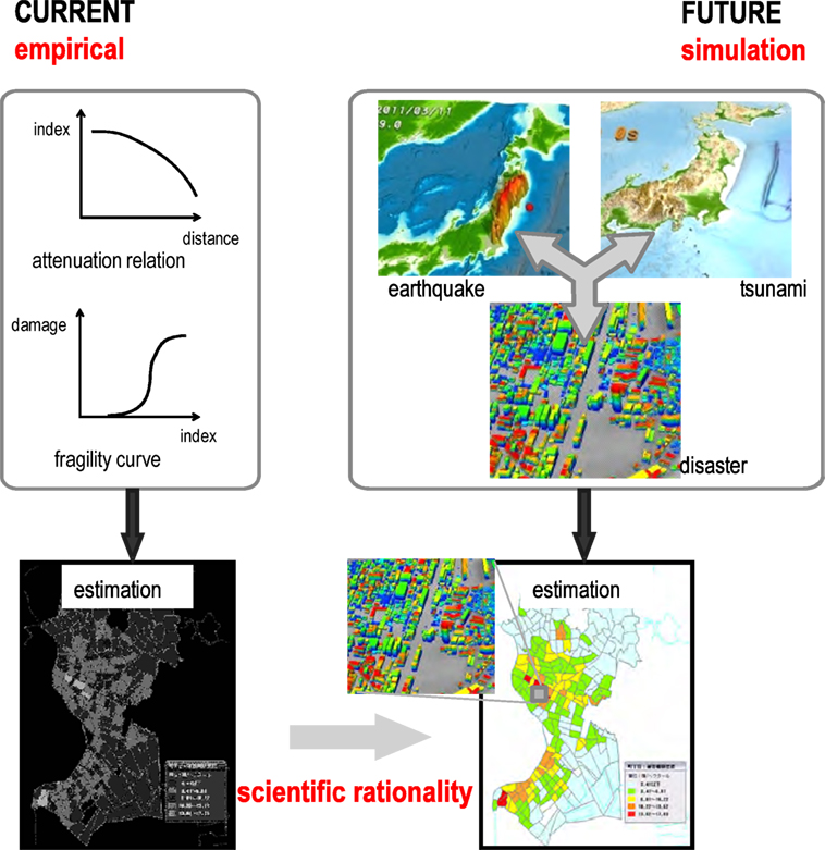
Figure 1. Methodology of estimating earthquake hazard and disaster.

While the question made above is natural, it is not easy to replace the empirical equations with the numerical simulation for the estimation of earthquake hazard and disaster. This is because there are two major difficulties; see Figure 2. The first difficulty is that simulating the propagation and amplification processes of seismic waves requires large-scale numerical computation if it needs high temporal and spatial resolution. The degree-of-freedom (DOF) increases as proportional to the inverse of the cubic of the spatial resolution (i.e., if the spatial resolution becomes half, DOF increases eight times), and the time step increases linearly to the required temporal resolution. The second difficulty is that an analysis model has to be constructed for each structure which is located in a target urban area. The number of the structures is of the order of 100,000, and an analysis model ought to have sufficient fidelity. The work needed for the model construction cannot be underestimated.

FIGURE 2

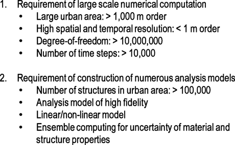
Figure 2. Two requirements in applying numerical simulation to estimation of earthquake hazard and disaster.

The authors have been developing a system for the estimation of earthquake hazard and disaster that uses a set of numerical analysis methods. Developing such a system is a challenging problem even for modern computational science since the target is an urban area. The system is called integrated earthquake simulation (Hori, 2011) (IES), as it integrates numerical analysis methods, together with modules for the automated model construction with which the implemented numerical analysis methods are executable. Key numerical simulations of IES are the simulation for the ground motion and the urban area seismic response. The ground motion simulation analyzes a three-dimensional underground structure model in which seismic waves are amplified in soft ground, and the urban area seismic response simulation computes a set of non-linear analysis models for all structures which are located in a target area.

This paper is aimed at summarizing recent achievements of developing IES, which are made by applying HPC to IES and using a large-scale parallel computer such as K computer in Japan (Miyamura et al., 2016). The contents of the present paper are organized as follows: first, in Section 2, we briefly explain the two difficulties in using numerical analysis method as an alternative of conventional empirical equations. The key features of IES are explained in Section 3; the architecture of IES for easier implementation of a third-party program is explained in detail. Examples of using IES for the earthquake hazard and disaster assessment are presented in Section 4. The target is Tokyo Metropolis, and the ground motion simulation and the urban area seismic response simulation made for this city by using K computer are explained.

In closing this section, we have to explain the quality of IES as numerical simulation. All the numerical methods that are implemented in IES are verified, but automatically constructed analysis models are not validated; literally no observed data are available for the purpose of validation. Highest quality is thus not expected for IES. The reliability of IES could be evaluated beside for the quality of the numerical simulation; IES employs the rational methodology of simulating the physical processes of earthquake hazard and disaster. No reduced models are used for the earthquake hazard estimation, and reduced but consistent models are sued for the earthquake disaster estimation. The resulting estimation of earthquake hazard and disaster made by IES is being compared with that made by the conventional method together with the observed data of 2011 Tohoku Earthquake.

2. Two Difficulties of Numerical Analysis for Earthquake Hazard and Disaster

The progress of computers, both hardware and software, enables us to utilize advanced numerical analysis methods in various fields of science and engineering. For instance, in the field of seismology, available are advanced numerical analysis methods which are capable to compute the seismic wave propagation processes in a large domain the dimension of which is in the crustal length scale (Bao et al., 1996; Somerville et al., 2001; Ichimura et al., 2009, 2014b; Yifeng et al., 2010; Cui et al., 2013; Quinay et al., 2013; Heinecke et al., 2014; Society, 2016; Tanaka et al., 2016). In earthquake engineering, numerical analysis methods based on finite element method (FEM) are being used to analyze soil–structure interaction effects for more accurate evaluation of seismic performance of a structure (Hori, 2011); material non-linearity of the structure and soil are considered in FEM.

The numerical analysis methods mentioned above are not capable to be used in the numerical simulation for the estimation of earthquake hazard and disaster in an urban area. As for the ground motion simulation, there is a limitation in the temporal resolution; the temporal resolution of currently available methods do not reach 10 Hz, which is needed for the accurate computation of structural responses since its major frequency components lie in the range of 1–10 Hz. Near the surface ground, the wave velocity is of the order of 100 m/s, and hence the required spatial resolution is 1 m in order to accurately compute frequency components of 10 Hz which has the wave length of 10 m; this fine resolution is in contrast of the spatial resolution of 100 m that is required for bedrock whose wave velocity is of the order of 1,000 m/s. Accurate computation is essential to estimate the topographical effects of irregular underground structures.

As for the urban area seismic response simulation, we have to construct an analysis model for all structures which are located in a target area. The quality of the constructed analysis model ought to be assured so that the results of the numerical analysis are reliable. Manual construction is not feasible for structures the number of which exceeds 100,000. Moreover, we have to be aware of the fact that perfect digital data about material and structural properties are not available for all the structures. For instance, high-rise buildings have a complete data set for the material and structure components for the construction, but the data set are not open to the public because the buildings are private asset.

We have to mention that the difficulty of constructing an analysis model is shared by the ground motion simulation. This is because the simulating needs a three-dimensional underground structure model which consists of a few soil layers of distinct configuration and material properties. The model must have high fidelity for the configuration of the soil layers, so that the topographical effects are evaluated accurately. However, the data of the soil layers are limited in the quality and quantity. We have to guess as well for the analysis model of the underground structures.

3. Solutions to Two Difficulties of Numerical Analysis

The first difficulty, the requirement of large-scale numerical computation, is solved by making use of HPC. A model of more than 10,000,000 DOF can be analyzed by using a parallel computer of moderate class, and we need to develop a numerical analysis method which possesses sufficient performance or fast analysis of a model of such large DOF. In IES, we have developed an FEM that is capable to solve a model of 1,000,000,000,000 DOF. Numerically solving a mode of this scale is a challenge in the field of HPC; this is regarded as a challenge of capability computing that solves a problem of largest scale. The number of time steps that are needed for the ground motion simulation is of the order of 10,000, since the time increment and the time duration are 0.01 and 100 s, respectively. FEM of IES is fast in analyzing a model of large DOF in repeated times.

The second difficulty, the need of analysis model construction for a large number of structures located in a target urban area, is solved by developing a program of the automated model construction. Automated model construction is regarded as data conversion, in the sense that digital data stored in several data resources are processed to form a set of digital data which correspond to an analysis model. Data resources available to the automated morel construction are of the form of Geographical Information System (GIS), and hence the data conversion is principally possible. As explained in the preceding section, however, there are no GIS’s which have data of the material and structure properties for all structures. We have to guess these properties by interpreting data which are stored in several data resources of GIS.

In the following two subsections, we briefly explain FEM developed for the ground motion simulation and the automated model construction for the urban area response simulation. The points of the explanation are the key feature of FEM and the automated model construction, in order to solve the two difficulties.

3.1. FEM Developed for IES

We first mention that FEM, rather than finite difference method, is suitable to solve numerical problems of the ground motion simulation, since a major concern of the simulation for the estimation of earthquake hazard is the identification of sites at which larger ground motion is concentrated due to the topographical effects induced by the underground structures. An analysis model of high fidelity is thus needed to model complicated configuration of soil layers, and FEM is the unique solution to analyze such a model.

The major portion of the numerical computation of FEM is used in solving a matrix equation for unknown displacement. That is,

$\begin{array}{c}\left(\frac{4}{d{t}^2}[M]+\frac{2}{dt}[C^n]+[K^n]\right)[\delta u^n]\\ =[f^n]-[q^{n-1}]+[C^n][v^{n-1}]+[M]\left([a^{n-1}]+\frac{4}{dt}[v^{n-1}]\right),\end{array}$ (1)

where [u], [v], [a], [f], and [q] are displacement, velocity, acceleration, external force, and residual force vectors, respectively; [M], [C], and [K] are mass, damping, and stiffness matrices, dt is the time increment, and superscript n stands for the n-th time step; [C] and [K] change due to non-linearity of soil. In the present paper, we employ a simple Ramberg–Osgood model and Masing rule (Ichimura et al., 2007; Lu and Guan, 2017) for the soil non-linearity. We compute [K] using the non-linear constitutive relations at all the Gauss points and compute [C] assuming a simple Rayleigh damping (Ichimura et al., 2015). The unknown is [δ uⁿ] = [uⁿ] − [uⁿ⁻¹], and [fⁿ] is given; the other matrices and vectors are determined. The ground motion simulation must solve a matrix equation the dimension of which is 1,000,000,000,000 for time steps of more than 10,000; for simplicity, [Cⁿ] and [Kⁿ] are fixed at the n-th time step, and the number of the time steps becomes a few times larger if [Cⁿ] and [Kⁿ] are changed at the same time step.

FEM of IES has developed a fast solver (Golub and Ye, 1997; Rietmann et al., 2012) which solves the matrix equation. The solver is tuned for K computer; the speed-up for the strong scalability is almost ideal, and the peak performance is 10 to 15% of the peak performance of K computer, depending on the number of compute nodes. Pre-conditioned conjugate gradient (CG) method is used as an algorithm of solving equation (1) for [δ uⁿ]; denoting by N the dimension of [δ uⁿ], the computation time is O(N²) for ordinary algorithms, but O(N log N) for the CG method. Note that the CG method is an iterative solver, as it computes a series of improved solutions for the matrix equation until it reaches a suitable solution which does not produce a large error of the matrix equation.

The speed of solving equation (1) by the pre-conditioned CG method depends on the number of iteration at which a suitably accurate solution is obtained as well as the CPU time of solving each iteration. Applying suitable pre-conditioning and using a good initial solution makes most efficient combination of the number of iteration and the CPU time for each iteration. To this end, we have to make special tunings in order to increase the performance of the solver; see the related references (Ichimura et al., 2014a, 2015; Agata et al., 2016; Fujita and Ichimura, 2016; Fujita et al., 2016) for detailed explanations of the tunings made by our group. The following two major tunings are made: (1) the geometric multi-grid which uses coarse and fine solutions (a coarse solution of less DOF and serves an initial solution for a fine solution of full DOF) and (2) the mixed precision arithmetic which uses single and double precision for the coarse and fine solution, respectively. In general, single precision arithmetic makes faster computation, and hence using single precision for parts of numerical computation which do not need high accuracy makes efficient numerical computation.

The scalability of the solver that is implemented in FEM of IES is presented in Figure 3; K computer is used for this computation, and DOF of the models analyzed exceeds 100,000,000. As the number of CPU cores increase, the CPU time decreases linearly, which indicates good scalability of the developed solver. We have to mention that other tunings, such as element-by-element method for efficient memory usage, compressed row storage for efficient communication, or predictor of higher order, are made for FEM of IES. The use of the element-by-element method reduces the number of elements for which an element stiffness matrix computes is computed, and the compressed row storage is used for the global stiffness matrix that is made by assembling those element stiffness matrices.

FIGURE 3

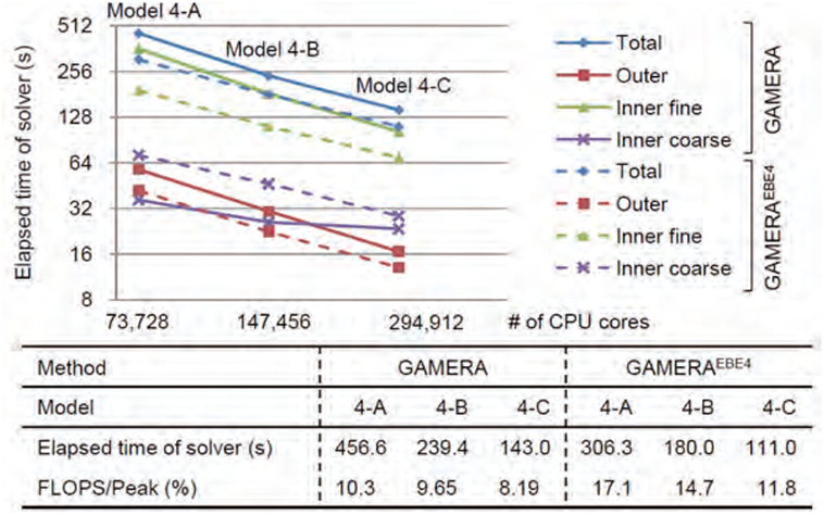
Figure 3. Scalability of developed FEM: GAMERA and GAMERA^EBE designate the usage of the element-by-element method (GAMERA does not use it); Model 4-A, 4-B, and 4-C have different DOF; outer, inner fine, and inner coarse provide the breakdown of the developed multi-grid solver processes, with outer for the finest grid with double precision arithmetic’s, inner fine and coarse for the coarse grid with single and double precision arithmetic’s, respectively.

3.2. Automated Model Construction Developed for IES

The automated model construction has two steps, namely, interpreting data stored in data resources, and converting data of the data resources to an analysis model (Architectural Institute of Japan, 2011); procedure (Idriss et al., 1978; Hori et al., 2015) of automatically constructing mutually consistent models for a target structure is proposed by our group, as well as procedure (Midorikawa et al., 2011; Taborda and Bielak, 2011; Miyamura et al., 2015) of constructing a highest fidelity model. A system of taking these steps for the automated model construction is being developed for IES. While the key simulations are the ground motion simulation and the urban area seismic response simulation, IES is implementing the seismic wave propagation simulation, the tsunami inundation simulation, and the mass evacuation simulation, which also need the automated model construction. Hence, the system ought to be flexible so that it is able to handle various numerical analysis models.

Data resources which are currently available are commercial GIS or 3D maps, or a set of inventories operated by local government. The commercial GIS has configuration data for structures including residential buildings and road networks. The configuration data are the height and floor shape of the structure, together with the location information of a target of the data, which is given as a pair of latitude and altitude. There are some structures whose configuration data include minor errors, such as negative height. The inventories are made for specific purposes such as the registration of real estate. There are the inventories for the structure type and construction year. The location information of a target structure is given as a certain address; mailing address or lot number is mainly used, but some inventories are made as a map and the location information is specified as coordinates of the map.

Interpreting data stored in a data resource is made by understanding the data structure of the data resource. In general, the data resource has several attributes (or data) to each target item, and the data structure means the number of attributes and the property of each attribute; there are cases where an attribute consists of a few attributes. Location information is an attribute. If the data structure is understood, it is possible to make a program for reading a file of the data resource (which is often of binary format) and interpreting data. Since data resources share a similar data structure, aspect-oriented programming makes efficient and robust programming for the program for reading and interpreting, when not a small number of data resources are used.

The difficulty of converting interpreted data to an analysis model depends on the complexity of the model. That is, a fewer model parameters are converted from the interpreted data, as a simpler model is constructed. The simplest model for the structural seismic response analysis is a linear one-degree-of-freedom system, which has two model parameters, a mass and a stiffness. The quality of the model depends on the accuracy of the model parameters, and we have to make rational conversion from the interpreted data to the model parameters. A natural frequency is a key characteristic of a structure, and an empirical relation between the natural frequency and the structure height is available (Architectural Institute of Japan, 1978; NIED, 2016). In IES, the natural frequency computed for the analysis model using the model parameters is compared with the empirical relation, in order to verify the reliability of the model that is constructed in an automated manner.

Between the step of interpreting data stored in data resources and converting data to an analysis method, we have to combine data for a target structure which are stored in different data resources. If the data include the location information of a target structure in it, combining the data is principally straightforward. However, as explained above, we have to interpret the location information in order to accurately specify the location of a target; this could be understood as conversion of the local coordinate (that is relevant to each data resource) to the global coordinate. There are data resources which have errors about location information or cases where contracting location information is found in different data resources. Combining data of different data resources for one structure is thus difficult, and manual works are needed if data resources which do not have accurate location information in them are used. A flow of the automated model construction is presented in Figure 4.

FIGURE 4

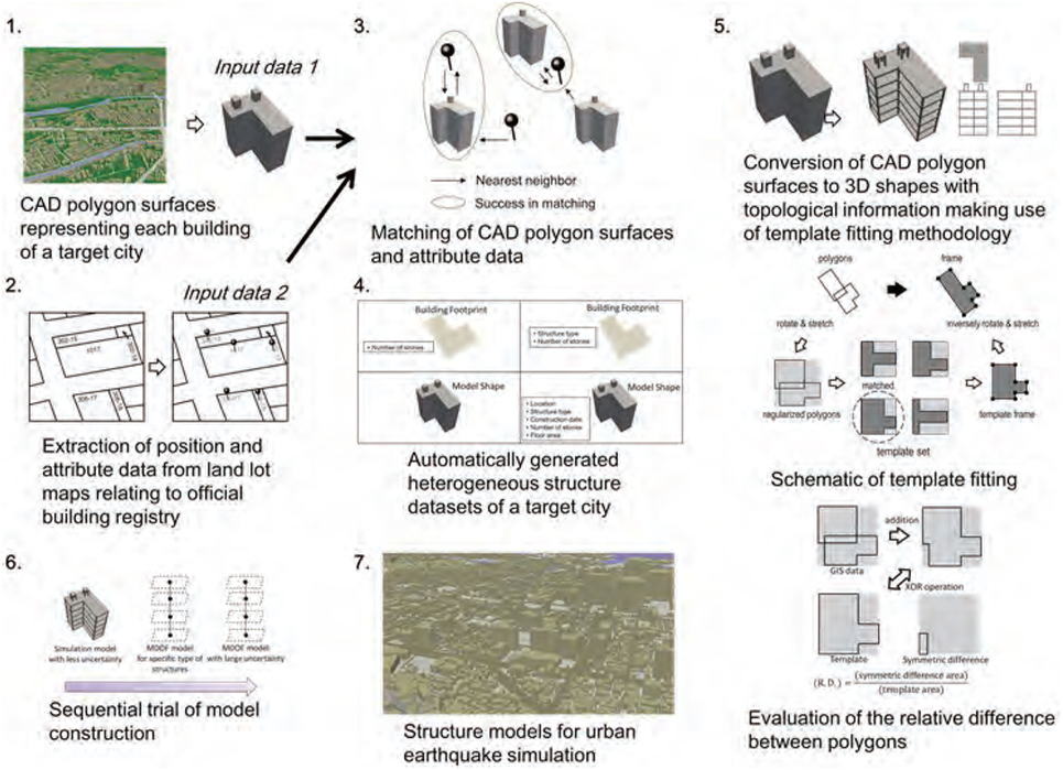
Figure 4. Flow of automated model construction.

We point out that the automated model construction system is designed for easy operation; the system is coded to take advantage of object-oriented programming together with the aspect-oriented programming. As shown in Figure 5, two built-infunctions, MakeShape and MakeAttribute, are used to interpret data stored in any data resource. Shape and Attribute are an object for the structure configuration and the structure properties (such as structure type, construction year), respectively. Another built-in function, MakeInputForP, is used to construct an analysis model for a program P of the structural seismic response analysis. As is seen, an analysis model for P is constructed by using data resources for which MakeShape and MakeAttribute are programmed.

FIGURE 5

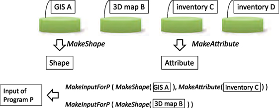
Figure 5. Two built-in functions of automated model construction system of IES.

It is not expected that complete information that is needed to construct an analysis model is included in available data resources. To account for the limitation of the available data, IES is able to construct 10,000 or more analysis models for one structure, which are generated by the automated model construction system, suitably varying model parameters. It is another challenge of HPC in terms of capacity computing to construct and analyze numerous models for one target considering the uncertainty of the model parameters; note that the number of analysis models reaches 10,000,000,0000 if IES analyzed 1,000,000 structures located in a target area and constructs 10,000 analysis models for each structure.

3.3. Uncertainty Quantification of IES

As mentioned, all the numerical analysis methods implemented in IES are verified by comparing the numerical solution with analytical solution, but automatically constructed analysis models are not validated. This is because no data are available to fully validate high fidelity model for the underground structure or numerous analysis models of buildings. Thus, IES cannot have highest quality as numerical analysis. Uncertainty quantification is needed for IES.

The greatest uncertainty is an earthquake scenario. Since predicting fault mechanism (or rupture processes on a fault plane) is impossible at this moment, an alternative is to simulate earthquake hazard and disaster for numerous earthquake scenarios. Indeed, capacity computing of HPS is often used for this purpose. Strong ground motion and structural seismic responses change depending on the given scenario, but we can quantitatively estimate a range of possible ground motion and seismic responses which are obtained by capacity computing.

As for man-made structures, we can use capacity computing in which numerous analysis models are used for one structure by changing model parameters. We might use 10,000 models for one structure. It should be noted that even when design data are available, actual structural properties are better than the design values since safety factors are included in the design. Monitoring or sensing is needed for the estimation of the actual structural properties; it is extremely difficult to estimate strength of a structure, compared with its stiffness, since strength is not identified until certain failure takes place in the structure.

4. Examples of IES Using High Performance Computing

In this section, we present examples of IES using capability computing and capacity computing. The target is Tokyo Metropolis, and commercial GIS’s are used as data resources. The ground motion simulation is made for an underground structure consisting of three ground layers, and the urban area seismic response simulation is made by using a non-linear multi-degree-of-freedom system as an analysis model of a residential building. The last example presents the combination of the ground motion simulation and the urban area seismic response simulation.

4.1. Ground Motion Simulation

An analysis model of surface layers is presented in Figure 6; the domain is 1,250 m × 1,250 m, and consists of three layers including bedrock (Miyazaki et al., 2012; SimCenter, 2016). The number of nodes, elements, and degree-of-freedom are 340,876,783, 252,737,051, and 1,022,630,349, respectively; this large scale of this model is necessary in order to assure the numerical convergence of the solution with temporal resolution up to 10 Hz (Housner, 1952; Ichimura et al., 2015; Ohtani et al., 2014). This simulation is regarded as capability computing, as DOF of the model exceeds 100,000,000. As mentioned, a simple Ramberg–Osgood mode and Masing rule are employed as a non-linear constitutive relation of soil (Ichimura et al., 2007; Lu and Guan, 2017).

FIGURE 6

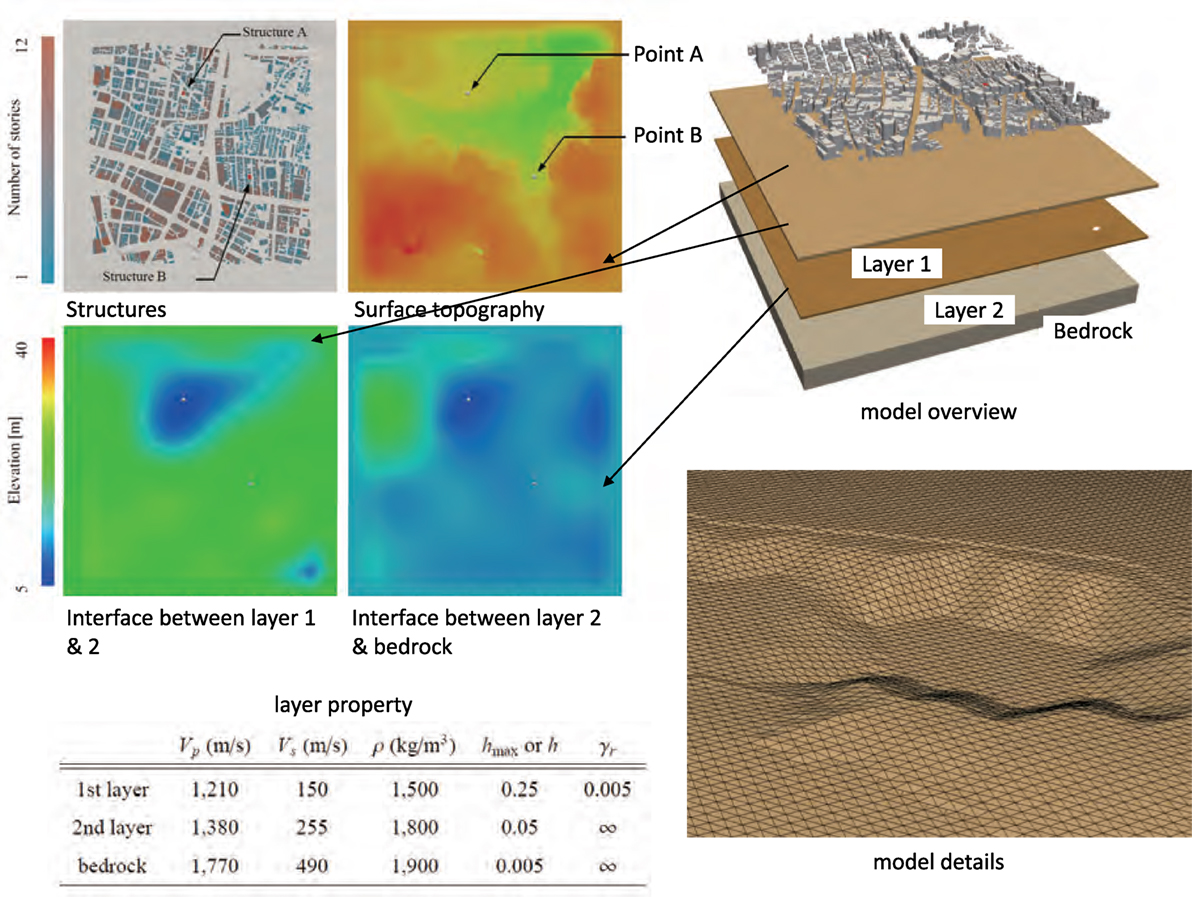
Figure 6. A model for ground motion simulation.

Figure 7 presents the distribution of SI (Tiankai et al., 2006), which is commonly used in earthquake engineering and defined as

$SI=\frac{1}{2.4}{\displaystyle {\int }_{0.1}^{2.5}}{S}_v(T)\text{d}T,$

with S_ν being the velocity response spectra of the ground motion measured or synthesized at the site; as is seen, SI is the average of the velocity response taken over 0.1 and 2.4 s. Kobe Earthquake (JR Takatori) (Japan Meteorological Agency, 2016) is used as input seismic wave on the bed rock. The distribution of SI is far from being uniform in this area of around 1 km × 1 km. As well expected, this is due to the topographical effects of the three layers of complicated configuration; see Figure 6. Recall that the uniform seismic wave is input on the bottom of the bedrock layer. There are two sites at which SI is concentrated; the value of SI exceeds 200 kine.

FIGURE 7

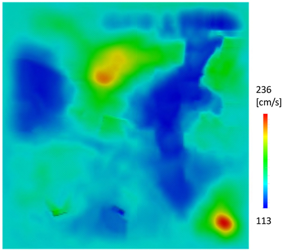
Figure 7. Distribution of SI.

It is of interest to compare the results of the above capability computing with the conventional analysis that uses a one-dimensional (1D) stratified model at a target site. In Figure 8, the waveform of acceleration in the EW and NS directions is presented; Points A and B indicated in Figure 6 are used for the comparison. While the waveform at Point B computed by the conventional analysis appears similar to that of the 3D model analysis, with the largest difference being around 30 Gal, the difference in the waveform at Point A is substantial with the largest difference being around 100 Gal. The dependence of the difference on the site is well excepted since Point A is located near the valley of the underground structure and has larger topographical effects on the ground motion concentration. It should be emphasized that capability computing that uses a large-scale model of underground structures enable us to understand the site and degree of the ground motion concentration induced by the topographical effects.

FIGURE 8

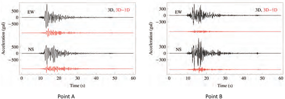
Figure 8. Comparison of ground motion simulation and conventional 1D analysis.

4.2. Urban Area Seismic Response Simulation

There are 4,066 residential buildings in the area presented in Figure 6. No inventory of the building type is available, and we assume that the structure type of all the buildings is reinforced concrete. A non-linear multi-degree-of-freedom system is made for each residential building; the number of the mass coincides with the floor number and a bi-linear spring is used to connect two neighboring masses. The mass is computed by using the floor area and an assumed floor thickness. The bi-linear spring has a linear relation between displacement and force until the force reaches the maximum value; the spring carries the same force even though its displacement increases. The stiffness for the linear relation is determined from an empirical equation between the first natural frequency and the building height.

The distribution of the maximum story drift angle (MSDA) is presented in Figure 9. It is difficult to see similarity in the distribution of SI and the distribution of MSDA, by comparing Figures 7 and 9. MSDA is relatively smaller at the two spots where SI is locally large and building models which have larger maximum drift angles stand at sites where SI is relatively smaller. The discrepancy between the ground motion concentration and the structural response is due to the difference in the dominant frequency of the ground motion input to the structure and the natural frequency of the structure. As for the earthquake hazard estimation, the distribution of MSDA is more important. We have to understand that relatively large MSDA is computed for a structure for which the coalesce of the input ground motion and its dynamic characteristic occurs.

FIGURE 9

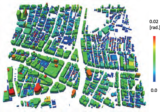
Figure 9. Distribution of MSDA.

Like the preceding subsection, we examine the necessity of making the 3D ground motion simulation, which provide ground motion that is amplified in ground layers and input to a structure on it. The identical analysis models are used for the residential buildings, but input ground motion is either the one computed by using the 3D ground motion simulation or the conventional 1D analysis. The results are presented in Figure 10; SI computed by the 3D ground motion simulation and the conventional 1D analysis, and the difference in SI are plotted in the top three figures, and MSDA based on the 3D ground motion simulation and the conventional 1D analysis, and the difference in MSDA are plotted in the bottom three figures. The difference reaches 40 kine for SI and 0.003 for MADA. This difference is critical; we need the ground motion simulation for the assessment of earthquake hazard and disaster at least in places which have larger topographical effects.

FIGURE 10

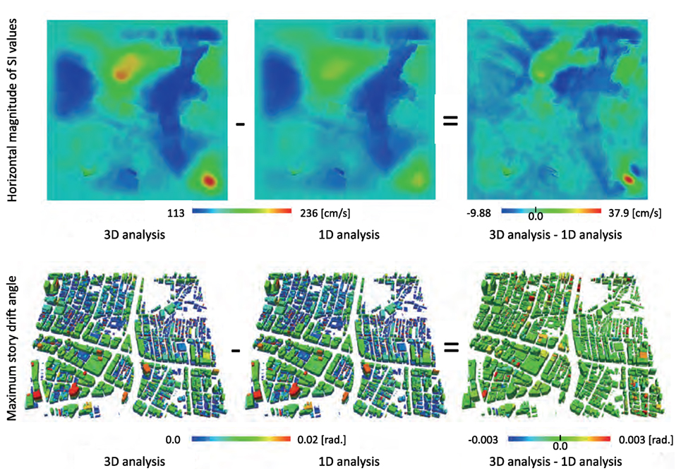
Figure 10. Comparison of ground motion simulation and conventional 1D analysis for estimation of earthquake hazard and disaster.

Due to the lack in relevant data resources, there is larger uncertainty in determining the strength of an analysis model for the residential buildings. While the stiffness can be determined by using empirical relations, it is not easy to determine the maximum force of the springs; the maximum force corresponds to the sum of the strength of walls and columns located on the floor which the spring represents. We apply capacity computing of generating 10,000 models for each residential building, assuming a normal distribution of the strength and assigning a randomly generated value to each spring; the mean of the maximum force is determined by using an empirical relation between the stiffness and the strength, and the SD is assumed to be 10% of the mean. Since the number of the buildings is 4,066, the total number of non-linear analysis models is 40,066,000.

A typical distribution of MSDA for 10,000 analysis models is shown in Figure 11. Three ground motions are used, and a wider distribution of MSDA is observed for larger ground motion. In Figure 12, the mean, the maximum, and the SD of MSDA is plotted. The effects of the model parameter uncertainty on the structural seismic response could be evaluated by studying the SD of MSDA. The SD of the model parameter (10% of the mean of the strength) produces the standard deviation of around 0.01 for MSDA when the largest ground motion is input. For this case, the non-linearity of the present analysis model induces a wider range of a possible earthquake disaster, compared with the uncertainty of the model parameter.

FIGURE 11

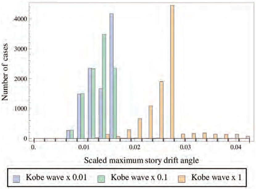
Figure 11. Distribution of MSDA for 10,000 analysis models for one residential building.

FIGURE 12

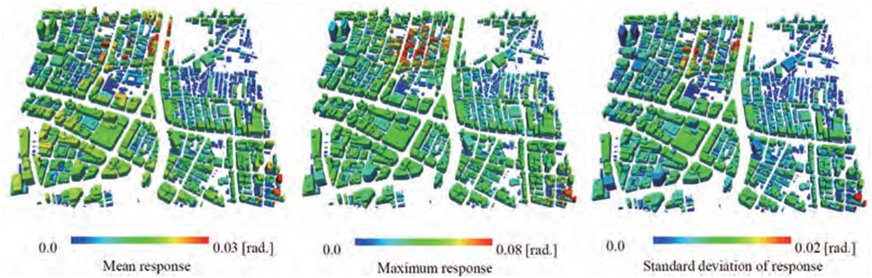
Figure 12. Distribution of mean, maximum and SD of MSDA.

4.3. Combined Simulation of Ground Motion and Urban Area Seismic Response Simulation for 10 km × 10 km Area

Using K computer, IES is able to mate the ground motion simulation and the urban area seismic response simulation for a domain of 10,250 m × 9,250 m (Ichimura et al., 2014a). This is the combined simulation in the sense that output of the ground motion simulation is used as input of the urban area seismic response simulation. It should be noted that the ground motion simulation is regarded as capability computing since it needs the whole 705,024 compute cores of K computer to finish the computation less than 12 h. An underground structure model similar to the one shown in Figure 6 is considered; it consists of three surface layers, but the number of DOF is 133,000,000,000 and the number of time steps is 6,600. In this setting, the temporal resolution is 10 Hz, which is assured by examining the convergence of a solution with respect to the model size.

An example of the combined simulation is presented in Figure 13; there are 32,800 residential buildings in the target domain, and a multi-degree-of-freedom system is constructed as an analysis model for each building, based on an assumption that they are a reinforced concrete building. The input ground motion is actually computed by using FEM for an assumed earthquake scenario of Tokyo Metropolis Earthquake (Government of Japan Cabinet Office, 2016). In IES, the earthquake hazard and disaster are quantified in terms of SI and MSDA, respectively. The distribution of these two indices is computed by making the combined simulation.

FIGURE 13

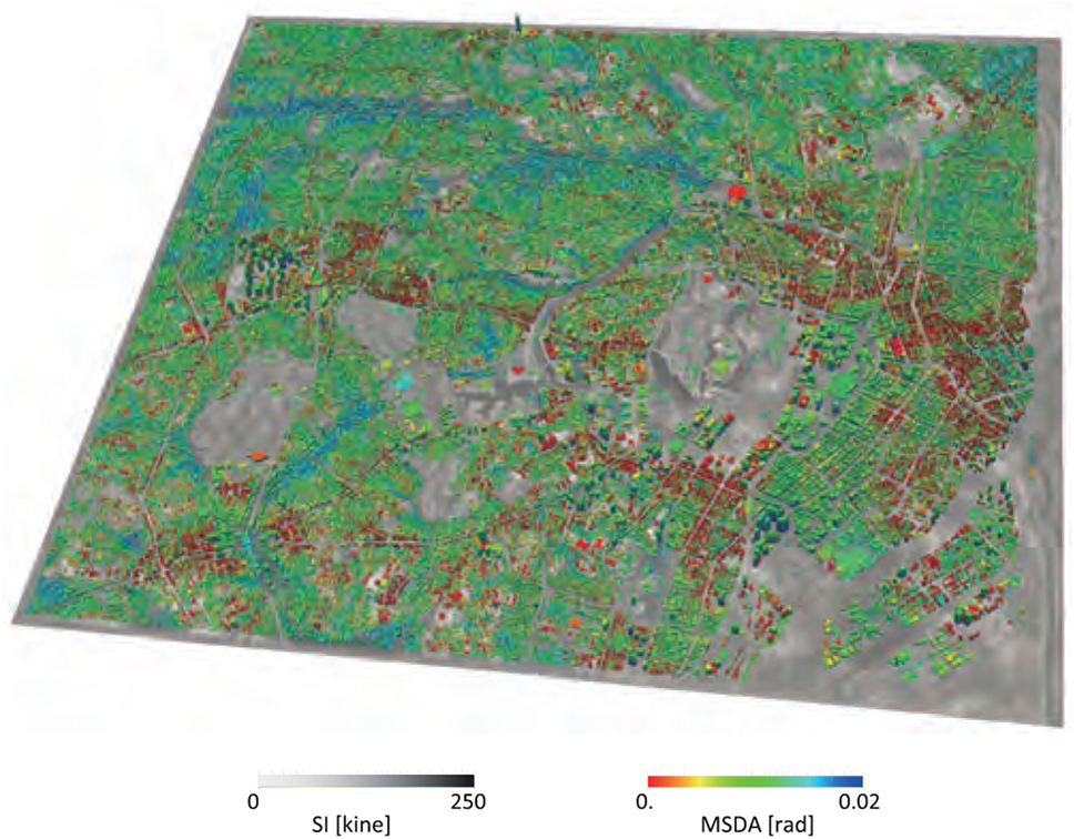
Figure 13. Distribution of SI and MSDA computed by making combined simulation of ground motion and seismic response.

It should be emphasized that new findings are never made in the combined simulation of IES. It simply combines ground motion simulation to well-established structural seismic response analysis. However, applying the combined simulation to a large area, we can surely identify spots at which SI takes on a larger value and other spots at which buildings of large MSDA’s are more densely located. The results of the combined simulation are worth being examined as it produces more rational assessment of earthquake hazard and disaster in highest resolution. Such combined simulation made by IES is applicable to any other cities in the world if suitable data resources are available and the automated model construction system generates a suitable model for the city using the data resources.

5. Concluding Remarks

This paper presents recent achievement of developing Integrated Earthquake Simulation (IES), by taking advantage of High performance computing (HPC). Indeed, IES enhanced with HPC enables us to develop a method of making a rational estimation of earthquake hazard and disaster for Tokyo Metropolis when an earthquake scenario is given. Provided that suitable computational environment and data resources are available, IES is applicable to any urban area. The two difficulties of numerically simulating earthquake hazard and disaster processes are being solved by developing a finite element method (FEM) with a fast solver and by developing a system of automated model construction.

We are planning to extend IES to social science simulations, such as mass evacuation from tsunami, traffic simulation in damaged areas, or recovery of economic activities. This social science simulation needs numerous scenarios of earthquake disasters which are made by applying IES to a target area for various earthquake scenarios. Further spatial resolution will be needed to consider more details of earthquake disasters, and we have to improve FEM of IES. It is another challenge to apply HPC to realize the social science simulation that is needed to increase the resilience of a target area, as it helps us to consider a better recovery plan. Part of the results was obtained by using the K computer at the RIKEN Advanced Institute for Computational Science. We used KiK-net and Japan Seismic Hazard Information Station of National Research Institute for Earth Science and Disaster Prevention (NIED), and National Digital Soil Map provided by Japanese Geotechnical Society. This work was supported by JSPS KAKENHI Grant Number 25220908, MEXT’s program of Post-K project.

Author Contributions

The first author is a primary investigator of this research. The second and third authors made numerical analysis programs for earthquake hazard and disaster assessment. The fourth, fifth, and sixth authors carried out numerical computations, constructing urban area models.

Conflict of Interest Statement

The authors declare that the research was conducted in the absence of any commercial or financial relationships that could be construed as a potential conflict of interest.

The reviewer, TI, declared a shared affiliation, though no other collaboration, with several of the authors, MH, TI, and LW, to the handling editor.

Funding

Part of the results was obtained by using the K computer at the RIKEN Advanced Institute for Computational Science. Results are obtained using the K computer at the RIKEN Advanced Institute for Computational Science. We used KiK-net and Japan Seismic Hazard Information Station of National Research Institute for Earth Science and Disaster Prevention (NIED), and National Digital Soil Map provided by Japanese Geotechnical Society. This work was supported by JSPS KAKENHI Grant Number 25220908, MEXT’s program of Post-K project.

References

Agata, R., Ichimura, T., Hirahara, K., Hyodo, M., Hori, T., and Hori, M. (2016). Robust and portable capacity computing method for many finite element analyses of a high-fidelity crustal structure model aimed for coseismic slip estimation. Comput. Geosci. 94, 121–130. doi: 10.1016/j.cageo.2016.05.015

CrossRef Full Text | Google Scholar

Architectural Institute of Japan. (1978). Vibration Experiment of Building (in Japanese). Maruzen.

Google Scholar

Architectural Institute of Japan. (2000). Damping of Building (in Japanese). Maruzen.

Google Scholar

Architectural Institute of Japan. (2011). Prompt Report on the 2011 Off the Pacific Coast of Tohoku Earthquake Disaster. Maruzen.

Google Scholar

Bao, H., Bielak, J., Ghattas, O., O’Hallaron, D. R., Kallivokas, L. F., Shewchuk, J. R., et al. (1996). “Earthquake ground motion modeling on parallel computers,” in The 1996 ACM/IEEE Conference on SUPERCOMPUTING, (Pittsburgh: IEEE Computer Society Press). doi:10.1145/369028.369053

CrossRef Full Text | Google Scholar

Cimellaro, G. P., Renschler, C., and Bruneau, M. (2014). Introduction to Resilience-Based Design, Computational Methods, Seismic Protection, Hybrid Testing and Resilience in Earthquake Engineering. New York: Springer International Publishing AG.

Google Scholar

Cui, Y., Poyraz, E., Olsen, K. B., Zhou, J., Withers, K., Callaghan, S., et al. (2013). “Physics-based seismic hazard analysis on petascale heterogeneous supercomputers,” in The International Conference on High Performance Computing, Networking, Storage and Analysis (SC’13) (New York: IEEE Computer Society Press). doi:10.1145/2503210.2503300

CrossRef Full Text | Google Scholar

DesignSafe-CI. (2016). Nheri: A Natural Hazards Engineering Research Infrastructure. Available at: https://www.designsafe-ci.org/about/designsafe/

Google Scholar

Fujita, K., and Ichimura, T. (2016). Development of large-scale three-dimensional seismic ground strain response analysis method and its application to Tokyo using full k computer. J. Earthq. Tsunami 10:1640017. doi:10.1142/S1793431116400170

CrossRef Full Text | Google Scholar

Fujita, K., Yamaguchi, T., Ichimura, T., Hori, M., and Maddegedara, L. (2016). “Acceleration of element-by-element kernel in unstructured implicit low-order finite-element earthquake simulation using openacc on pascal gpus,” in Third Workshop on Accelerator Programming Using Directives (WACCPD, WACCPD’ 16), Salt Lake City. doi:10.1109/WACCPD.2016.6

CrossRef Full Text | Google Scholar

GEM. (2015). Openquake: Global Earthquake Model. Available at: https://www.globalquakemodel.org/

Google Scholar

Golub, G. H., and Ye, Q. (1997). Inexact preconditioned conjugate gradient method with inner-outer iteration. SIAM J. Sci. Comput. 21, 1305–1320. doi:10.1137/S1064827597323415

CrossRef Full Text | Google Scholar

Government of Japan Cabinet Office. (2016). Report of the Assumed Tokyo Large Earthquake Model Committee. Available at: http://www.bousai.go.jp/kaigirep/chuobou/senmon/shutochokkajishinmodel/

Google Scholar

HAZUS. (2017). Hazus 4.0. Available at: http://www.hazus.org/

Google Scholar

Heinecke, A., Breuer, A., Rettenberger, S., Bader, M., Gabriel, A.-A., Pelties, C., et al. (2014). “Petascale high order dynamic rupture earthquake simulations on heterogeneous supercomputers,” in The International Conference on High Performance Computing, Networking, Storage and Analysis, (SC’14) (New Orleans, LA: IEEE Computer Society Press), 3–14. doi:10.1109/SC.2014.6

CrossRef Full Text | Google Scholar

Hori, M. (2011). Introduction to Computational Earthquake Engineering, 2nd Edn. London: Imperial College Press.

Google Scholar

Hori, M., Wijerathne, L., Ichimura, T., and Tanaka, S. (2015). Meta-modeling for constructing model consistent with continuum mechanics. J. Jpn. Soc. Civil Eng. Ser. A2 71. doi:10.2208/journalofjsce.2.1_269

CrossRef Full Text | Google Scholar

Housner, G. W. (1952). “Spectrum intensity of strong motion earthquakes,” in Proceedings of the Symposium on Earthquakes and Blast Effects on Structures (California: Earthquake Engineering Research Institute), 20–36.

Google Scholar

Ichimura, T., Fujita, K., Hori, M., Sakanoue, T., and Hamanaka, R. (2014a). Three-dimensional nonlinear seismic ground response analysis of local site effects for estimating seismic behavior of buried pipelines. J. Press. Vessel Technol. Am. Soc. Mech. Eng. 136:041702. doi:10.1115/1.4026208

CrossRef Full Text | Google Scholar

Ichimura, T., Fujita, K., Tanaka, S., Hori, M., Lalith, M., Shizawa, Y., et al. (2014b). “Physics-based urban earthquake simulation enhanced by 10.7 BlnDOF x 30 k time-step unstructured fe non-linear seismic wave simulation,” in The International Conference on High Performance Computing, Networking, Storage and Analysis (SC’14) (New Orleans, LA: IEEE Computer Society Press), 15–26. doi:10.1109/SC.2014.7

CrossRef Full Text | Google Scholar

Ichimura, T., Fujita, K., Quinay, P. E. B., Maddegedara, L., Hori, M., Tanaka, S., et al. (2015). “Implicit nonlinear wave simulation with 1.08t DOF and 0.270t unstructured finite elements to enhance comprehensive earthquake Simulation,” in The International Conference for High Performance Computing, Networking, Storage and Analysis (SC’15) (New Orleans, LA: IEEE Computer Society Press). doi:10.1145/2807591.2807674

CrossRef Full Text | Google Scholar

Ichimura, T., Hori, M., and Bielak, J. (2009). A hybrid multiresolution meshing technique for finite element three-dimensional earthquake ground motion modeling in basins including topography. Geophys. J. Int. 177, 1221–1232. doi:10.1111/j.1365-246X.2009.04154.x

CrossRef Full Text | Google Scholar

Ichimura, T., Hori, M., and Kuwamoto, H. (2007). Earthquake motion simulation with multi-scale finite element analysis on hybrid grid. Bull. Seismol. Soc. Am. 97, 1133–1143. doi:10.1785/0120060175

CrossRef Full Text | Google Scholar

Idriss, I. M., Singh, R. D., and Dobry, R. (1978). Nonlinear behavior of soft clays during cyclic loading. J. Geotech. Eng. 104, 1427–1447.

Google Scholar

Japan Meteorological Agency. (2016). Strong Ground Motion of the Southern Hyogo Prefecture Earthquake in 1995 Observed at Kobe JMA Observatory. Available at: http://www.data.jma.go.jp/svd/eqev/data/kyoshin/jishin/hyogo_nanbu/index.html

Google Scholar

Jayasinghe, J. A. S. C., Tanaka, S., Wijerathne, L., Hori, M., and Ichimura, T. (2015). Automated construction of consistent lumped mass model for road network. J. Jpn. Soc. Civil Eng. 71, I_547–I_556. doi:10.2208/jscejseee.71.I_547

CrossRef Full Text | Google Scholar

Lu, X., and Guan, H. (2017). Earthquake Disaster Simulation of Civil Infrastructures, from Tall Buildings to Urban Areas. New York: Springer.

Google Scholar

Masing, G. (1926). “Eigenspannungen und verfestigung beim messing (in German),” in The 2nd International Congress of Applied Mechanics, 332–335.

Google Scholar

Midorikawa, S., Ito, Y., and Miura, H. (2011). Vulnerability functions of buildings based on damage survey data of earthquakes after the 1995 kobe earthquake. J. Jpn. Assoc. Earthq. Eng. 11, 4_34–4_47. doi:10.5610/jaee.11.4_34

CrossRef Full Text | Google Scholar

Miyamura, T., Akiba, H., and Hori, M. (2015). Large-scale seismic response analysis of super-high-rise steel building considering soil-structure interaction using k computer. High Rise 4, 75–83.

Google Scholar

Miyamura, T., Tanaka, S., and Hori, M. (2016). Large-scale seismic response analysis of a super-high-rise-building fully considering the soil-structure interaction using a high-fidelity 3d solid element model. J. Earthq. Tsunami 10:1640014. doi:10.1142/S1793431116400145

CrossRef Full Text | Google Scholar

Miyazaki, H., Kusano, Y., Shinjou, N., Shoji, F., Yokokawa, M., and Watanabe, T. (2012). Overview of the k Computer System, Vol. 48, FUJITSU Sci. Tech, J, 302–309.

Google Scholar

NIED. (2016). Japan Seismic Hazard Information Station, National Research Institute for Earth Science and Disaster Prevention. Available at: http://www.j-shis.bosai.go.jp/en/

Google Scholar

Ohtani, H., Chen, J., and Hori, M. (2014). Automatic combination of the 3D shapes and the attributes of buildings in different GIS data. J. Jpn. Soc. Civil Eng. Ser. 70, I_631–I_639. doi:10.2208/jscejam.70.I_631

CrossRef Full Text | Google Scholar

Quinay, P. E. B., Ichimura, T., Hori, M., Nishida, A., and Yoshimura, S. (2013). Seismic structural response estimates of a high-fidelity fault-structure system model using multiscale analysis with parallel simulation of seismic wave propagation. Bull. Seismol. Soc. Am. 103, 2094–2110. doi:10.1785/0120120216

CrossRef Full Text | Google Scholar

Rietmann, M., Messmer, P., Nissen-Meyer, T., Peter, D., Basini, P., Komatitsch, D., et al. (2012). “Forward and adjoint simulations of seismic wave propagation on emerging largescale GPU architectures,” in The International Conference on High Performance Computing, Networking, Storage and Analysis (SC’ 12) (Los Alamitos: IEEE Computer Society Press).

Google Scholar

Saad, Y. (2003). Iterative Methods for Sparse Linear Systems, 2nd Edn. New York: SIAM.

Google Scholar

Sahin, A., Sisman, R., Askan, A., and Hori, M. (2016). Development of integrated earthquake simulation system for Istanbul. Earth Planets Space 68, 115. doi:10.1186/s40623-016-0497-y

CrossRef Full Text | Google Scholar

Si, H., and Midorikawa, S. (1999). New attenuation relationships for peak ground acceleration and velocity considering effects of fault type and site condition. J. Struct. Construct. Eng. 523, 63–70.

Google Scholar

SimCenter. (2016). Computational Mdoeling and Simulaiton Center. Available at: https://www.designsafe-ci.org/facilities/simcenter/

Google Scholar

Society, T. J. G. (2016). National Digital Soil Map. Available at: http://www.denshi-jiban.jp/

Google Scholar

Somerville, P., Collins, N., Abrahamson, N., Graves, R., and Saikia, C. (2001). Ground Motion Attenuation Relations for the Central and Eastern United States, Final Report. Available at: http://earthquake.usgs.gov/hazards/products/conterminous/2008/99HQGR0098.pdf

Google Scholar

Taborda, R., and Bielak, J. (2011). Large-scale earthquake simulation: computational seismology and complex engineering systems. Comput. Sci. Eng. 13, 14–27. doi:10.1109/MCSE.2011.19

CrossRef Full Text | Google Scholar

Tanaka, S., Hori, M., and Ichimura, T. (2016). Hybrid finite element modeling for seismic structural response analysis of a reinforced concrete structure. J. Earthq. Tsunami 10:1640015. doi:10.1142/S1793431116400157

CrossRef Full Text | Google Scholar

Tiankai, T., Hongfeng, Y., Ramirez-Guzman, L., Bielak, J., Ghattas, O., Kwan-Liu, M., et al. (2006). “From mesh generation to scientific visualization: an End-to-end approach to parallel supercomputing,” in The 2006 ACMIEEE conference on Supercomputing (SCf06) (New York: ACM). doi:10.1145/1188455.1188551

CrossRef Full Text | Google Scholar

Yifeng, C., Cui, C., Olsen, K. B., Jordan, T. H., Lee, K., Zhou, J., et al. (2010). “Scalable earthquake simulation on petascale supercomputers,” in The 2010 ACM/IEEE International Conference for High Performance Computing, Networking, Storage and Analysis (SC’10) (Washington: IEEE Computer Society), 1–20. doi:10.1109/SC.2010.45

CrossRef Full Text | Google Scholar