Rapid and Automated Damage Detection in Buildings Through ARMAX Analysis of Wind Induced Vibrations

Introduction

When a building undergoes a seismic event, the typical method for locating and analyzing any potential structural damage involves lengthy surface level visual inspections by structural engineers where each critical member is classified in a damage category based on the engineer's judgement. Such an arbitrary inspection method often leads to inconclusive and inconsistent damage analysis.

To overcome the issues from visual inspections, vibration-based structural health monitoring (SHM) has seen substantial progress due to the rapid development of advanced technologies in the areas of computer science and electrical engineering; it is now more convenient and cheaper to acquire large amounts of data. Despite this abundant data, the proper way to detect damage is still a big challenge.

Among all the vibration-based SHM methods, non-parametric methods and statistical pattern recognition techniques, such as Time Series Modeling (Sohn et al., 2001; Nair et al., 2006; Gul and Catbas, 2009, 2011) have gained significant momentum in the field of SHM due to their ability to deal with massive data and their capability to improve reliability by accounting for the variations in the recorded data.

Time series analysis is used to analyze time dependent data sets to understand their statistical characteristics. In their infancy, time series models were not used for structural analysis purposes. They were initially used in a variety of fields, such as population modeling, electrical engineering, long term weather predictions, and stock price prediction. In the following papers, the coefficients of time series models are used as damage sensitive features in which damage was found by comparing the changes in the coefficients from the undamaged and damaged models. Bodeux and Golinval (2000) introduced the application of Vector Autoregression Moving-Average (VARMA) models for both system identification and damage detection. Their approach utilized a prediction error method which assumed a zero mean Guassian white noise. The method was tested on the “Steel-Quake” benchmark proposed in the framework of COST Action F3 “Structural Dynamics.” The tests showed a good correlation for the modal parameters and for detecting damage based on the modal parameter uncertainties, however the location of the damage was not properly identified. Gul and Catbas (2011) implemented a novel damage detection process which involved creating a damage detection model which combined time series modeling and a novel sensor clustering technique. The authors created ARX models for different sensor clusters by using the free response of the structure and each sensor cluster output was treated as an input for the ARX model. The methodology was shown to successfully identify and locate damage on both numerical and experimental vibration data even when noise is considered. Nair et al. (2006) introduced a new damage sensitive feature (DSF) using the first three auto-regressive (AR) terms from the auto-regressice moving average (ARMA) series that is modeled from vibrations. The authors found that the mean values of the DSF for the damaged and undamaged signals were different, so a statistical summarization, i.e., a t-test, was implemented to obtain a confident damage decision. Numerical and experimental vibration data from the ASCE benchmark was used to validate the method and the results showed that both minor and major damage could be precisely detected and located. de Lautour and Omenzetter (2006) analyzed the vibrations of a multi story building due to ground motion to detect seismic damage within the building. Their simple numerical 3 story structure was subjected to random ground motion and the resulting vibrations at each story were fit to an AR time series model. The AR coefficients were then used as the inputs for an Artificial Neural Network (ANN). The ANN was trained to detect any changes in the AR coefficients from before and after damage to identify and quantify the damage at each story. The results from their numerical case study proved that their methodology could successfully detect damage in a simple numerical structure even in the presence of noise and changes in operating conditions. Ji et al. (2011) conducted a series of full scale tests at the E-Defense shaking table facilities to simulate realistic seismic damage in a high-rise steel building. In conducting these full scale tests, the authors could evaluate the effectiveness of vibration-based damage diagnosis methodologies using real life vibration data. The vibration data from each floor was fit by the frequency response curve-fitting method and the ARX method. As the seismic damage increased, the natural frequencies of the structure decreased as expected. The modal shapes, however did not change as the damage was distributed evenly over the height of the structure. Note that these results only apply to steel high rise structures and it is expected that different results would occur if a different type of structure was used, such as a concrete moment frame or shear wall structure. Bao et al. (2013) proposed a damage detection technique for subsea pipelines which could account for various loading conditions. The authors first partitioned and normalized the acceleration data, then used auto-correlation functions and partial-correction functions to compute the ARMA models inputs and their orders, respectively. The AR parameters served as the damage feature vector and the damage indicators were based on the Mahalanobis Distance between the ARMA models which were used for damage detection and localization. A finite element model of a subsea pipeline under ambient excitations was numerically simulated to verify the authors' methodology, and the results show that it can successfully detect and locate damage even with noise effects. Roy et al. (2015) proposed a set of 4 ARX model based DSF for damage detection and localization when no input excitation data is made available. This was done by assuming that one of the output responses in a multi-degree-of-freedom (MDOF) system is assumed as an input whereas the rest are taken as the output. The damage features are based on ARX model coefficients, Kolmogorov-Smirnov test statistical distance, and the model residual error. The authors' methodology was tested on both numerical and experimental structures and the results show that the DSF could both localize and quantify the stiffness degradation, however, in cases where there are multiple locations of damage, one of the DSFs was unable to clearly quantify the amount of stiffness degradation. Lakshmi and Rama Mohan Rao (2014) created a novel output-only damage detection technique based on time series analysis which accounted for environmental variability and measurement noise. The authors applied Principle Component Analysis to transform the large amount of data in order to reduce the data size, thereby improving computational efficiency. The data is fitted with AR and ARX models, and the probability density functions of damage features are obtained by assessing variance in prediction errors. The authors tested their methodology on a numerical simply supported beam and an experimental three story framed bookshelf benchmark structure. Results from the experiments indicate that the method can detect and locate damage, however the measurement of the severity of damage should be further examined.

This article presents an automated SHM system based on Time Series Analysis (TSA) and sensor clustering capable of rapidly providing engineers with the location and degree of damage at a story level precision from the building's vibration due to ambient wind forces. The method presented in this paper is developed based on previous studies of the authors (Mei and Gül, 2014; Do, 2015), and aims to complement lengthy visual inspections and arbitrary scaling constants to provide a more efficient, consistent and accurate damage assessment.

The novelty of the paper is to utilize structural responses under wind loading to rapidly detect damage in a building at a story level precision with severity information. When relating this damage detection methodology to the objectives presented by Rytter (1993), it satisfies the first three steps.

Methodology

Background to Time Series Models

This section provides a brief discussion about the Auto-Regressive Moving Average model with eXogenous inputs (ARMAX). More discussions about time series model theories can be found in the following literature (Sohn and Farrar, 2001; Lu and Gao, 2005; Omenzetter and Brownjohn, 2006).

ARMAX modeling is the specific time series model used in this paper. Its general form is given in Equation (1).

$\begin{array}{l}y(t)+a_{1}y(t-\Delta t)+\dots +a_{n_a}y(t-n_a\Delta t)\\ =b_{0}u(t)+b_{1}u(t-\Delta t)+\dots +b_{n_b}u(t-n_b\Delta t)+e(t)\\ +d_{1}e(t)+d_{1}e(t-\Delta t)+\dots +d_{n_c}e(t-n_c\Delta t)& (1)\end{array}$

In Equation (1), y(t) is the output, u(t) is the input of the model, e(t) is the error term, and a_i, b_i, d_i are the parameters of the model. The model orders are given in terms of n_a, n_b, n_c. A general form of the ARMAX equation can be written as Equation (2).

$\begin{array}{ll}A(q)y(t)=B(q)u(t)+D(q)e(t)& (2)\end{array}$

The terms A(q), B(q) and D(q) are polynomials in delay operators q^j as shown in Equation (3).

$\begin{array}{l}A(q)=1+a_1{q}^{-1}+\dots +a_{n_a}{q}^{-n_a}\\ B(q)=b_1{q}^{-1}+b_2{q}^{-2}+\dots +b_{n_b}{q}^{-n_b}\\ D(q)=1+d_1{q}^{-1}+\dots +d_{n_c}{q}^{-n_c}& (3)\end{array}$

From Equation (3), it is simpler to understand the meaning of the delay operator. For example, a data set x(t) at time multiplied by q^j is equal to x(t – jΔt). From the general form of the ARMAX models (Equation 2), different time series models can be created by changing the order of A(q), B(q), and D(q). For example, Auto Regressive (AR) process is created with only n_a while n_b, and n_c are set to zero. The Moving Average (MA) process sets n_a and n_b to zeros and a non-zero value to n_c. The ARX model is defined as setting n_c to zero. As previously stated, the focus of this paper will be solely on ARMAX modeling of the transformed equations of motion as described below.

ARMAX Models for Different Sensor Clusters

The equation of motion, which governs the dynamic responses (accelerations, velocities and displacements) of structures, is described herein. Equation (4) below represents the general equation of motion for an N degree of freedom system.

$\begin{array}{ll}\text{M}ẍ(\mathrm{\text{t}})+\text{C}ẋ(\mathrm{\text{t}})+\text{K}x(\mathrm{\text{t}})=f(\mathrm{\text{t}})& (4)\end{array}$

In which M, C and K represent the N by N mass, damping and stiffness matrices of the system. The vectors ẍ(t), ẋ(t), and x(t) represent the acceleration, velocity and displacement at a certain time t. The external forcing vector is denoted by f (t) which is considered as a wind force in this paper. The vibration of a structure is strongly dependent on time, the prior state of the structure, and external inputs. By modeling the vibration data as a time series sequence, statistical characteristics of the time series which represents the behavior of the structure can be extracted. This vibration data can be gathered by installing a pair of bi-axial sensors in perpendicular directions at each story. The focus of this research centers on the change in stiffness which represents damage within the lateral resisting members of a building structure.

Equations (5–12) outline the steps for how the equation of motion (EOM) can be transformed so that it can be represented as an ARMAX model. For clarity, one story (represented as a single degree of freedom) is considered as a single i^th row in Equation (4) and is shown in Equation (5) below.

$\begin{array}{l}(m_{i1}{ẍ}_1(t)+\dots +m_{iN}{ẍ}_N(t))+(c_{i1}{ẋ}_1(t)+\dots +c_{iN}{ẋ}_N(t))\\ +(k_{i1}{x}_1(t)+\dots +k_{iN}{x}_N(t))=f_i(t)& (5)\end{array}$

Rearranging Equation (5) to isolate the acceleration on the left-hand side results in Equation (6).

$\begin{array}{l}{ẍ}_i=\frac{f_i}{m_{ii}}\\ -\frac{m_{i,1}{ẍ}_1+\dots +m_{i,i-1}{ẍ}_{i-1}+m_{i,i+1}{ẍ}_{i+1}+\dots +m_{i,N}{ẍ}_N}{m_{ii}}\\ -\frac{c_{i,1}{ẋ}_1+c_{i,2}{ẋ}_2+\dots +c_{i,N}{ẋ}_N}{m_{ii}}\\ -\frac{k_{i,1}{x}_1+k_{i,2}{x}_2+\dots +k_{i,N}{x}_N}{m_{ii}}& (6)\end{array}$

It can be assumed in shear type building modeling that the mass of each degree of freedom is entirely lumped into the center of the degree of freedom. Any mass values which aren't in the diagonal are assumed to be zero and can be removed. For simplicity, the damping terms in the equation can be removed due to their miniscule contribution to the equations balance. As such, Equation (6) can be simplified to Equation (7) below.

$\begin{array}{ll}{ẍ}_i=\frac{f_i}{m_{ii}}-\frac{k_{i,1}{x}_1+k_{i,2}{x}_2+\dots +k_{i,N}{x}_N}{m_{ii}}& (7)\end{array}$

Taking the second derivative of Equation (7) results in Equation (8) below.

$\begin{array}{ll}{\displaystyle \underset{i}{\overset{\dots .}{x}}}=\frac{{\ddot{f}}_i}{m_{ii}}-\frac{k_{i,1}{ẍ}_1+k_{i,2}{ẍ}_2+\dots +k_{i,N}{ẍ}_N}{m_{ii}}& (8)\end{array}$

The goal of taking the second derivative of Equation (8) is to create an equation in which the right-hand side is only dependent on acceleration values. Measuring the displacement and velocities of a structure under light ambient wind loading may result in measurement errors due to the miniscule values involved. By applying the forward difference technique (Levy and Lessman, 1961) as shown in Equation (9), the left side of Equation (8) can be transformed to create a new equation solely based on acceleration values as shown in Equation (10).

$\begin{array}{ll}{x}_i=\frac{{ẍ}_i(t+\Delta t)-{ẍ}_i(t)}{\Delta t}& (9)\end{array}$

$\begin{array}{l}{\displaystyle \underset{i}{\overset{\dots }{ẋ}}}=\frac{\frac{{ẍ}_i(t+2\Delta t)-{ẍ}_i(t+\Delta t)}{\Delta t}-\frac{{ẍ}_i(t+\Delta t)-{ẍ}_i(t)}{\Delta t}}{\Delta t}\\ \frac{\frac{{ẍ}_i(t+2\Delta t)-{ẍ}_i(t+\Delta t)}{\Delta t}-\frac{{ẍ}_i(t+\Delta t)-{ẍ}_i(t)}{\Delta t}}{\Delta t}\\ =\frac{{\ddot{f}}_i(t)}{m_{ii}}-\frac{k_{i,1}{ẍ}_1(t)+k_{i,2}{ẍ}_2(t)+\dots +k_{i,N}{ẍ}_N(t)}{m_{ii}}& (10)\end{array}$

One issue with the newly transformed Equation (10) is that the acceleration ẋ(t) exists on both sides of the equation, which could lead to trivial solutions. To eliminate this possibility, a new sequence y_i(t) is introduced to represent the left components in Equation (10) where y_i(t) = ẍ_i(t+Δt)−ẍ_i(t). The final transformation of the equation of motion is shown in Equation (11).

$\begin{array}{l}\frac{y_i(t+\Delta t)-y_i(t)}{\Delta t^2}=\frac{{\ddot{f}}_i(t)}{m_{ii}}\\ -\frac{k_{i,1}{ẍ}_1(t)+k_{i,2}{ẍ}_2(t)+\dots +k_{i,N}{ẍ}_N(t)}{m_{ii}}& (11)\end{array}$

This newly transformed equation can be represented as an ARMAX function (Equation 1) provided that y_i(t) and ẍ_i(t) are considered the output and input terms, respectively. The error term in the ARMAX model represents damping, excitation force, ambient noise and numerical errors out of the numerical approximation of the derivative. As stated in Do (2015), it was found that an order of 1 for both the n_a and n_b terms and an order of 3 for the n_c term was sufficient to account for these influences. The ARMAX model for the i^th row of the equation of motion of a multi-DOF system can be expressed as in Equation (12) below. The parameters can be estimated using least square criterion (Mei and Gül, 2016, #207).

$\begin{array}{l}{y}_i(t+\Delta t)+a^i{y}_i(t)=b_1^i{ẍ}_1(t)+b_2^i{ẍ}_2(t)+\dots +b_N^i{ẍ}_N(t)\\ +e(t)+d_1^{i}e(t-\Delta t)+d_2^{i}e(t-\Delta t)& (12)\end{array}$

Sensor Clustering

Due to the nature of shear structures, it can be assumed that the signal of a DOF can only affect the DOFs located directly above or below. With this assumption, the time series models can be constructed in a more concise way where each model only incorporates the neighboring DOFs. These models are referred to as a sensor cluster.

Based on the ARMAX model built for the equation of motion of a DOF, vibration at one sensor is chosen to fit the part at the left side of the equation, which is considered the reference channel. The vibration data from the neighboring sensors represent the right part of the equation. For an N-DOF structure, there are N ARMAX models with outputs as the reference channel and inputs only from the adjacent channels.

The ARMAX model is solely reliant on the sensor clusters, and not the readings of each individual sensor. This sensor clustering technique, which was previously developed by Gul and Catbas (2011), greatly reduces the complexity of the equation of motion for an N DOF.

If we consider a four story shear building to explain this sensor clustering technique. The first sensor cluster created to build the ARMAX model incorporates the first and second story and the first story is chosen as the reference channel. The reference channel of the second cluster is the second story, and the two neighboring stories (first and third) are included. The third sensor cluster has the third story as its reference channel and includes the two adjacent stories: the second and the fourth. The final sensor cluster incorporates both the third and fourth stories, with the fourth story being the reference channel.

Building Damage Features

Among the property changes of a shear structure, mass changes are often related to the loading of the structure and are not considered as damage in most cases. To isolate stiffness changes from mass changes, the damage features proposed by Do (2015) are used in this paper. This section briefly describes the definition of the damage features.

The B(q) terms in the ARMAX model (Equation 12) represents the terms $\frac{k_{ij}}{m_{ii}}$ in the equation of motions of each sensor cluster. The baseline case matrix is defined in Equation (13) and the matrix representing the unknown case (i.e., damaged case) is represented by Equation (14).

$\begin{array}{ll}{b}_{j,baseline}^i=\left[\begin{array}{cccc}{b}_1^1& b_2^1& \dots & b_n^1\\ b_1^2& b_2^2& \dots & b_n^2\\ ⋮& ⋮& \ddots & ⋮\\ b_1^n& b_2^n& \dots & b_n^n\end{array}\right]\cong \left[\begin{array}{cccc}\frac{k_{11}}{m_{11}}& \frac{k_{12}}{m_{11}}& \dots & \frac{k_{1n}}{m_{11}}\\ \frac{k_{21}}{m_{22}}& \frac{k_{22}}{m_{22}}& \dots & \frac{k_{2n}}{m_{22}}\\ ⋮& ⋮& \ddots & ⋮\\ \frac{k_{n1}}{m_{nn}}& \frac{k_{n2}}{m_{nn}}& \dots & \frac{k_{nn}}{m_{nn}}\end{array}\right]& (13)\end{array}$

$\begin{array}{ll}{d}_{j,damaged}^i=\left[\begin{array}{cccc}{d}_1^1& d_2^1& \dots & d_n^1\\ d_1^2& d_2^2& \dots & d_n^2\\ ⋮& ⋮& \ddots & ⋮\\ d_1^n& d_2^n& \dots & d_n^n\end{array}\right]\cong \left[\begin{array}{cccc}\frac{k{\prime }_{11}}{m{\prime }_{11}}& \frac{k{\prime }_{12}}{m{\prime }_{11}}& \cdots & \frac{k{\prime }_{1n}}{m{\prime }_{11}}\\ \frac{k{\prime }_{21}}{m{\prime }_{22}}& \frac{k{\prime }_{22}}{m{\prime }_{22}}& \cdots & \frac{k{\prime }_{2n}}{m{\prime }_{22}}\\ ⋮& ⋮& \ddots & ⋮\\ \frac{k{\prime }_{n1}}{m{\prime }_{nn}}& \frac{k{\prime }_{n2}}{m{\prime }_{nn}}& \cdots & \frac{k{\prime }_{nn}}{m{\prime }_{nn}}\end{array}\right]& (14)\end{array}$

During seismic event, reinforced concrete members will often undergo a reduction in stiffness. As such, this paper focuses only on the loss of stiffness in a structure to determine damage and the mass is assumed to have not changed significantly during the seismic event. Therefore, the denominators in Equation (14) can be changed from $m_{ij}^{\prime }$ to m_ij to produce a new matrix as shown in Equation (15), where the stiffness terms are the only ones which change between the baseline case and the unknown case.

$\begin{array}{ll}{d}_{j,damaged}^i\cong \left[\begin{array}{cccc}\frac{k{\prime }_{11}}{m_{11}}& \frac{k{\prime }_{12}}{m_{11}}& \cdots & \frac{k{\prime }_{1n}}{m_{11}}\\ \frac{k{\prime }_{21}}{m_{22}}& \frac{k{\prime }_{22}}{m_{22}}& \cdots & \frac{k{\prime }_{2n}}{m_{22}}\\ ⋮& ⋮& \ddots & ⋮\\ \frac{k{\prime }_{n1}}{m_{nn}}& \frac{k{\prime }_{n2}}{m_{nn}}& \cdots & \frac{k{\prime }_{nn}}{m_{nn}}\end{array}\right]& (15)\end{array}$

The Stiffness Damage Feature (SDF) is presented in Equation (16) as follows.

$\begin{array}{l}SDFs=\frac{d_{j,damaged}^i-b_{j,basline}^i}{b_{j,basline}^i}\times 100\%i:\mathrm{\text{sensor clusters}};\\ j:\mathrm{\text{adjacent sensors}}& (16)\end{array}$

Case Studies: Numerical Analysis

To verify the validity of the ARMAX damage detection model, two different structures were modeled using SAP2000. Each structure was subjected to a variety of damage cases, and the undamaged and damaged models' acceleration responses to ambient wind forces were analyzed and the SDFs were calculated. Those SDFs were then directly compared to the expected SDF results which were obtained from extracting the stiffness matrices from SAP2000.

Of the two of the structures modeled, one was a steel moment frame and the other was a reinforced concrete (RC) frame, where shear deformation from lateral loading is most prevalent. The ARMAX DDM assumes that the structures can be approximated as shear type structures and therefore flexural deflection are not considered.

Each structure is presented with damage cases which range from minor damage cases (only one story damaged) to severe damage cases (>70% of stories damaged). The entire procedure for the numerical analysis can be summarized through Figure 1.

FIGURE 1

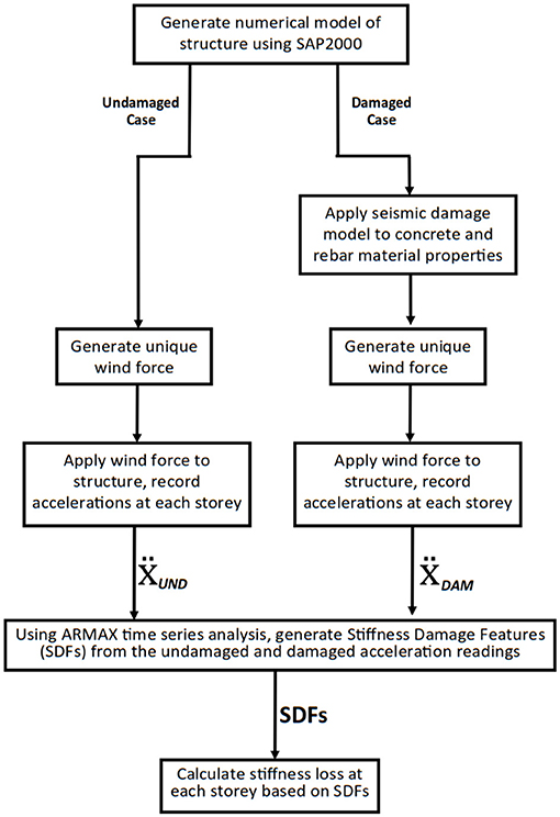
Figure 1. Damage model overview.

Wind Speed Simulation Model

The ARMAX DDM previously outlined requires acceleration readings at every story to properly function. As previously stated, the acceleration responses can be gathered by installing one bi-axial sensor per story. These accelerations are created by a lateral wind force acting on the building. The following sections describe the procedure to generate the wind forces.

Wind Simulation at Reference Elevation

When simulating a wind speed function, a common technique involves breaking the wind down to two components: the Low Frequency Component (LFC) which represents the average hourly wind speed; and the high frequency component (HFC) which considers the wind speeds at shorter time periods ranging from 10 to 300 s (Welfonder et al., 1997; Nichita et al., 2002; Bayem et al., 2008). This can be represented as follows:

$\begin{array}{ll}{U}_r(t)=v_{LFC}(t)+v_{HFC}(t)& (17)\end{array}$

This paper utilizes the method proposed by Fernandez and Alonso (2017) to create a wind speed model at a reference story elevation which considered both wind components as stochastic variables, greatly simplifying the wind speed simulation process and correlating excellently to real life measurements.

Wind Speeds at Other Elevations

When generating the wind speed functions for elevations other than the reference story elevation, two factors must be considered: the mean wind speed at the given elevation and the correlation with regards to the neighboring story wind speeds.

In general, wind speeds increase at higher heights. In this paper, Power Law is used to represent mean wind speed profiles at other elevations as it has shown to give an accurate approximation for elevations below 200 m (Holmes, 2015)

$\begin{array}{ll}U(z)=U_r\times {\left(\frac{z}{z_r}\right)}^{\alpha }& (18)\end{array}$

The exponent α is an empirically derived landscape coefficient that ranges from 0.10 for smooth, flat terrain to 0.40 for cities with high rise buildings (Bañuelos-Ruedas et al., 2010). The wind force example used for the two damage models had an exponent value of 0.30.

Correlation is defined as the real number in the range [-1, 1] that measures how two variables (i.e., wind speeds) at different elevations evolve with each other. The Pearson correlation equation (Pearson, 1895), which is used in this paper to measure correlation of wind speeds at different elevations, is defined in Equation (19).

$\begin{array}{ll}{\rho }_{xy}=\frac{{\sigma }_{xy}^2}{{\sigma }_x{\sigma }_y}& (19)\end{array}$

The correlation of real-life wind speeds will not be equal to one. The correlation generally ranges from 0.50 to 0.80 depending on site characteristics and wind speeds. The correlation is simulated based on Kim et al. (2009), which can best reflect real-life measurements.

$\begin{array}{ll}{C}_{12}(r_y,r_z,n)=e^{(-r^{*}\times n^{*})}& (20)\end{array}$

$\begin{array}{l}{r}^{*}=\frac{\sqrt{{(k_y{r}_y)}^2+{(k_z{r}_z)}^2}}{L_x(z_m)}\\ n^{*}=\sqrt{1+{(\frac{n{L}_x(z_m)}{k_{2}U(z_m)})}^2}\\ z_m=\sqrt{z_1\times z_2}\\ r_z=z_2-z_1\\ where{k}_y=0.5,k_z=0.5,k_2=0.06\end{array}$

In Equation (20) listed above, the only inputs required are the vertical and horizontal distances between two points (r_z and r_y, respectively) and the frequency at which wind speeds are taken (i.e., T_SAMPLE = 10 s, n = 0.1). With the power law and correlation effects accounted for, a wind speed model was generated in the following section which accounts for any elevation as it relates to the wind speed created in the previous section.

Wind Force Generation Model at a Given Elevation

The first step in creating a wind speed at a given elevation was to generate the wind speed at the reference elevation (first story) as shown in previously, as that reference elevation speed is the baseline for the second story wind speed. With the baseline wind speed generated, each story's wind speed was built in ascending order by first increasing each story's wind speed relative to the story below using the power law. Following that increase, a correlation generator was developed to model real life wind behavior.

According to Kim et al. (2009), the predicted correlation between wind speeds at 3.25 m height difference is 0.695. To simulate the correct correlation, a correlation generator was developed to induce some randomness by either increasing or decreasing the wind speed from its original value. The randomized numbers were bounded by a normal distribution with varying limits to create wind speed trials with varying correlation values. An iterative program was created which simulates several wind speed trials with different limits and then checks which trial yielded the optimal correlation value.

With the second story wind speed generated, the wind speed is then generated for the third floor using the same correlation generator procedure with the second story as the new reference elevation speed and with a different correlation value. This process is repeated for each story until each floor has a wind speed which corresponds to the Power Law mean speed and appropriate correlation. Afterwards, the simulation is refined further to account for turbulence at a one second wind speed samples.

An example final version of wind speeds at 10 separate stories is shown in Figure 2A which represents wind speeds with an average starting hourly wind speed of 4 m/s (~11 km/hr) at the first story.

FIGURE 2

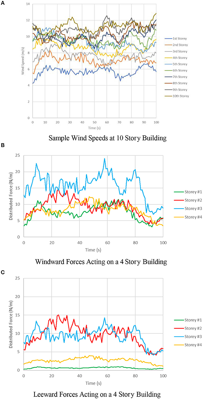
Figure 2. Sample wind forces. (A) Sample wind speeds at 10 Story building. (B) Windward forces acting on a 4 Story building. (C) Leeward forces acting on a 4 Story building.

The major factors that can affect the wind pressure include density of surrounding buildings, relative heights of surrounding buildings, surface roughness and angle of wind. A parametric model considering all the factors above proposed by Grosso (1992) was introduced to simulate pressure coefficients along the building. These pressure coefficients were used in conjunction with the calculated wind speeds to generate a story by story wind force which can be utilized during the damage detection model. A sample of windward and leeward distributed forces (6 m/s average wind speed) acting on a four story 16 m tall building are presented in Figures 2B,C. The windward and leeward forces were applied at the windward and leeward sides of each story's floor slab as uniform distributed loads in the numerical building models. The frequency spectrum of wind force and structural response are shown in Figure 3.

FIGURE 3

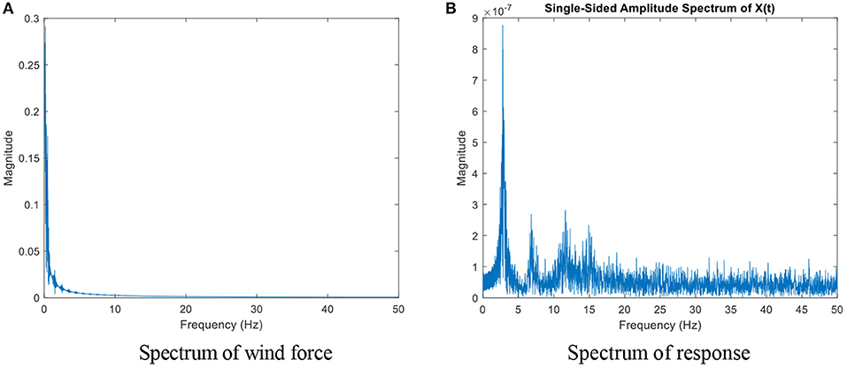
Figure 3. Spectra of wind force and response of a 4 Story Building. (A) Spectrum of wind force. (B) Spectrum of response.

Numerical Damage Modeling Technique

As the proposed methodology is based on its ability to detect damage in numerical building models, it is imperative that the damage properly reflects real life behavior. One of the most commonly used damage analysis technique to determine the degree of damage in a structure is the stiffness degradation method, which compares the initial loading stiffness slope of an undamaged structural member to the reloading stiffness slope after the member/structure is subjected to a seismic event. This stiffness degradation model will be utilized as it directly relates to the focus of the ARMAX DDM which determines the change in stiffness at a story by story level. To properly reflect damage, both the concrete and steel properties were modified as follows.

Concrete Damage

According to Guo et al. (2016), it was assumed that any stiffness reduction can be attributed to the degradation of the initial reloading modulus of concrete as shown in Equation (21). This assumption holds true because when the steel bars are unloaded and reloaded, their reloading modulus generally will not change drastically due to the elastic nature of steel, whereas the formation of cracks in concrete due to a seismic event would greatly reduce the reloading modulus. This damage model assumes that the concrete has underwent non-linear damage due to the concrete strain passing its peak strength value (~0.22%). Note that although the concrete has undergone non-linear damage, the ambient wind forces acting on the reinforced concrete afterwards would be of low enough force so that the “re-loaded” concrete is behaving in a linear fashion.

$\begin{array}{ll}D{R}_{Concrete}=1-\frac{E_{New}}{E_{original}}& (21)\end{array}$

Chang and Mander (1994) studied the effects of dynamic and cyclic loading on concrete and they developed a set of equations which can relate the original stiffness (E_ORIGINAL) to any reloading damaged stiffness (E_NEW) while also calculating the new stress and strain capacities. This set of equations proposed by Chang and Mander (1994) were adapted to create new concrete capacity curves in which the only inputs required are the original concrete compressive strength, initial flexural stiffness and the target Damage Ratio (DR).

The range of Damage Ratios spans from minor damage (0.40) to critical damage (0.65). Minor damage refers to the point in which cracks become noticeable in the concrete. Critical damage refers to the point just before complete failure of the concrete with zero force capacity. These Damage Ratio limits and corresponding degrees of damage were determined previously by Toussi and Yao (1983).

For illustrative purposes, the stiffness, ultimate strength and ultimate strain capacity of the undamaged and damaged 40 MPa concrete is presented in Table 1. It is assumed that the damaged concrete has lost all tensile capacity due to cracking.

TABLE 1

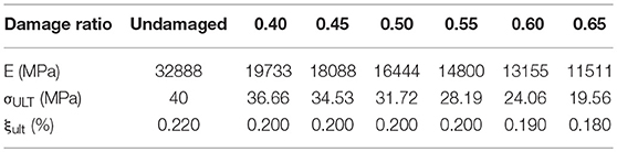
Table 1. Undamaged and damaged concrete material properties.

Figure 4 is presented below for better visualization and understanding of how the damaged concrete compressive curves compare to the undamaged concrete. Past a strain value of 0.37%, it is assumed that the concrete will have completely failed (Toussi and Yao, 1983). In this paper, concrete damage is introduced by changing the material characteristics, i.e., modulus of elasticity and peak compressive strength, of the damaged columns according to DR within the SAP2000 model.

FIGURE 4

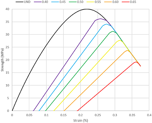
Figure 4. Concrete compressive strength curves.

Steel Damage

As the steel reinforcing bars undergo cyclic loading, the unloading and reloading modulus of elasticity remains relatively unchanged. What does change, however, is the ultimate strength of the steel, as the constant cyclic loading has a fatigue loading effect. As such, the DR of the reinforcing steel bars can be calculated as the ratio of the new ultimate strength of the steel compared to its undamaged ultimate capacity and is illustrated in Equation (22) below.

$\begin{array}{ll}D{R}_{Rebar}=1-\frac{{\sigma }_{Ult.(New)}}{{\sigma }_{Ult.(Original)}}& (22)\end{array}$

In this paper, steel members in SAP2000 are replaced with aluminum members to simulate damage.

Parameters

In this paper, a 4 story steel structure and a 10 story reinforced concrete structure are simulated. As an example, the procedure to calculate parameters of the 4 story steel structure is shown herein. The four story buildings is simplified as 4-DOF systems where the stiffness values of k₁ to k₄ are the lateral force resisting stiffness' at each floor and the mass is assumed to be lumped in the floor of each story. Each numerical building model is treated as a strong-beam weak-column structure and therefore the beams and slabs were treated as perfectly rigid. The stiffness and mass matrix of the first four stories are shown in Equations (23,24), respectively.

$\begin{array}{ll}K=\left[\begin{array}{cccc}{K}_{11}& K_{12}& K_{13}& K_{14}\\ K_{21}& K_{22}& K_{23}& K_{24}\\ K_{31}& K_{32}& K_{33}& K_{34}\\ K_{41}& K_{42}& K_{43}& K_{44}\end{array}\right]=\left[\begin{array}{cccc}{k}_1+k_2& -k_2& 0& 0\\ -k_2& k_2+k_3& -k_3& 0\\ 0& -k_3& k_3+k_4& -k_4\\ 0& 0& -k_4& k_4\end{array}\right]& (23)\end{array}$

$\begin{array}{ll}M=\left[\begin{array}{cccc}{m}_{11}& 0& 0& 0\\ 0& m_{22}& 0& 0\\ 0& 0& m_{33}& 0\\ 0& 0& 0& m_{44}\end{array}\right]& (24)\end{array}$

With the stiffness and mass matrices set up as shown, the stiffness damage feature (SDF) matrix was represented as follows. Note that the equation to calculate each SDF is shown in Equation (16).

$\begin{array}{ll}SDF=\left[\begin{array}{cccc}SD{F}_{11}& SD{F}_{12}& 0& 0\\ SD{F}_{21}& SD{F}_{22}& SD{F}_{23}& 0\\ 0& SD{F}_{32}& SD{F}_{33}& SD{F}_{34}\\ 0& 0& SD{F}_{43}& SD{F}_{44}\end{array}\right]& (25)\end{array}$

This methodology also applies to the 10 story structure, with the only difference being that the stiffness, mass and SDF matrices are represented as 10 × 10 matrices as opposed to 4 × 4 matrices. With the general SDF matrix set up, the overall loss in stiffness at each story can be calculated as in Equation (26). Note that “last story” refers to the highest story of the building and the calculation of ΔK₁ requires that K₁ = K₂.

$\begin{array}{l}\Delta K_1=(2\times SD{F}_{11})-\Delta K_2\\ \Delta K_i=\frac{SD{F}_{i-1,i}+SD{F}_{i,i-1}}{2},i=2,3,\dots ,n-1\\ \Delta K_n=\frac{SD{F}_{n-1,n}+SD{F}_{n,n-1}+SD{F}_{n,n}}{3}& (26)\end{array}$

Theoretically, the change in stiffness at each story (aside from the first) can be gathered by taking a single SDF value, however by averaging the value of two SDF values instead, the experimental errors were mitigated.

To better simulate real life scenarios in which the collected data are usually corrupted with measurement error, white noise with mean of 0 and standard deviation of 5% of original signal's standard deviation are added to each story's acceleration response during the baseline and damaged cases. The SDF results presented in the following section represent the average SDF values after performing 10 trials with the noisy data.

For each structure, the story accelerations were measured at the center of each floor slab. Throughout the numerical modeling simulations, the average starting hourly wind speeds on the first story ranged from 2 m/s (3.6 km/hr) to 8 m/s (28.8 km/hr).

The damage in each numerical model was represented as a uniform change in the material properties throughout an entire column. This model is slightly simplified, as it is expected in moment frames that the top and bottom of each column would be the most damaged due to the peak moment forces location.

For the RC building model, the building reinforcement is designed as per the Concrete Design Handbook-−4th Edition with the loads being calculated using the 2015 National Building Code of Canada (Cement Association of Canada and Canadian Standards Association, 2016). The structures are assumed to be conventional office buildings in Vancouver on Soil Type D. The building reinforcement was verified through SAP2000's automated moment frame design calculations.

The structural response due to wind for the RC model was calculated using Newmark's direct integration method (γ = 0.25, β = 0.50) and incorporated proportional damping with a constant 7% damping coefficient for baseline state of structure and a 5% damping coefficient for the unknown state of the structure (Newmark, 1982). The concrete compressive curves were modeled using Mander's curve.

The material specifications for the structural steel, concrete and rebar are presented in Table 2.

TABLE 2

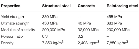
Table 2. Properties for materials.

Case Studies: Results and Discussion

To verify the validity of the ARMAX damage detection model, two numerical building models are presented below. The wind was sampled at 100 Hz and the total time period for one state of each structure is 10 s. Each structure was subjected to a variety of damage cases, and the undamaged and damaged models' acceleration responses to ambient wind forces were analyzed and the SDFs were calculated. It should be mentioned here again that a 5% artificial noise was added to all the responses obtained from the models. Those SDFs were then directly compared to the expected SDF results which were obtained from extracting the stiffness matrix from SAP2000. The ARMAX DDM assumes that the structures can be approximated as shear type structures and therefore flexural deflection are not considered. Each structure is presented with damage cases which range from minor damage cases (only one story damaged) to severe damage cases (>70% of stories damaged).

Case Study I: 4 Story Steel Structure

It was imperative that the finite element (FE) modeling parameters were properly calibrated to simulate real life structural behavior. As such, the first structure considered was a replica of an experimental four story steel structure which was built by Do (2015). The FE model replica was subjected to identical damage cases to those verified in the experiments to verify that the FE model parameters used throughout this paper properly reflect real life damage from previously created experiments. The focus on steel structure was not to detect seismic damage in a structure, it was to ensure that the numerical modeling parameters reflected real life behavior.

The 3D view and plan view of the structural model are shown in Figure 5. As each steel angle column is identical in material properties and dimensions, they are all considered to have identical stiffness values.

FIGURE 5

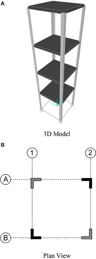
Figure 5. FE Model for steel structure. (A) 3D model. (B) Plan view.

To validate that the FE model can be replicated to match previous experiments, the structure was excited by two pairs of Multiple Impulse Forces (MIF) located at the two corners of the first and third floors. This forcing function was created through randomly generating an impulse force under normal distribution at every 0.1 seconds.

The acceleration response of the structure from the MIF was recorded at 0.001 s intervals. For the steel structure, the response calculated by FE modeling was a linear modal response using a constant damping of 2%.

The original accelerations for the first sensor cluster are presented in Figure 6. It is seen that the value of output is generally twice smaller than input data. This makes sense because the output is the difference of acceleration. It is expected that such small inconsistency in terms of order is unlikely to cause the ill-conditioning of matrix while estimating the parameters. As for this sensor cluster, the number of predicted points is 499 and the number of unknowns is 5, i.e., ($a^1,b_1^1,b_2^1,d_1^1\mathrm{\text{and}}{d}_2^1$).

FIGURE 6

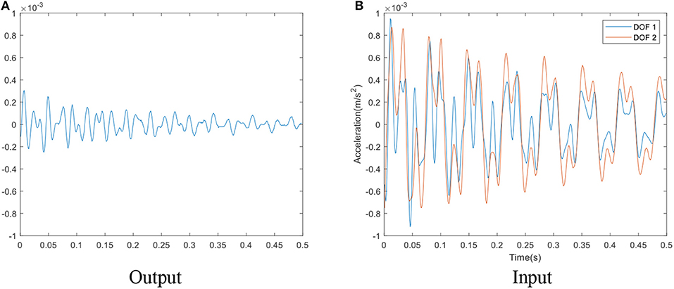
Figure 6. Original accelerations of the first sensor cluster of healthy case of case study 1. (A) Output. (B) Input.

Damage Case S1—Single Story Damage (4th Story)

The first damage case involved replacing one of the steel angle columns with an identically sized aluminum angle column at the fourth story. The location of the damaged column is at A1 as shown in Figure 5B.

By replacing a 200 GPa steel column with a 63 GPa aluminum column at location A1 (the intersection of gridline A and gridline 1), the Damage Ratio of the single column was 1 – (63/200) = 0.685. Every other column in the structure was unchanged and therefore can be assumed to have Damage Ratio of 0. The overall loss in stiffness on the fourth story can be calculated as [((3 × 0) – (1 × 0.685))/4] = −17.13% which would be reflected in SDF₃₄, SDF₄₃, SDF₄₄; SDF₃₃, which represents the change in combined stiffness of the third and fourth story can be calculated as [((7 × 0) – (1 × 0.685))/8] = −8.56%. Note that the denominator represents the total number of columns that are included in each respective SDF.

To validate this calculation method, each expected SDF is confirmed through extracting the stiffness matrix of the finite element (FE) models. The extracted FE results (also referred to as the “expected” results) and the ARMAX analysis results; one case with no noise and one with 5% noise added; are presented in Table 3 below. Throughout the damage cases, the SDF results represent the average of 10 trials.

TABLE 3

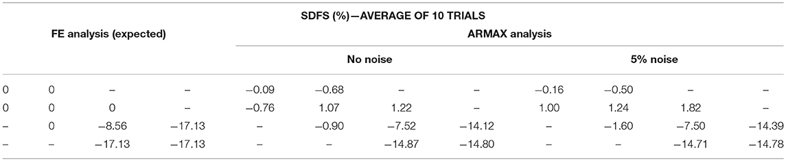
Table 3. SDF results (DC S1).

The 5% noise effect did not have a significant impact on the SDF values from the ARMAX analysis. With the SDF matrix set up, the overall loss in stiffness in each story was calculated as shown in Equation (26) using the 5% noise SDF values. The calculated change in stiffness at each story from the ARMAX DDM is presented in Equation (27). For brevity, these calculations will not be shown for any other damage case.

$\begin{array}{l}\text{Story}1:(2\times (-0.16))-(0.25)=-0.57\%\\ \text{Story}2:((-0.50)+(1.00))/2=+0.25\%\\ \text{Story}3:((1.82)+(-1.60))/2=+0.11\%\\ \text{Story}4:((-14.39)+(-14.71)+(-14.78))/3=-14.63\%& (27)\end{array}$

The overall change in stiffness of each story based on the 5% noise SDF values from the 10 trials are presented in Table 4. The bracketed values in the ARMAX column represent the standard deviation of the 10 trials, with a lower standard deviation value signifying more stable results.

TABLE 4

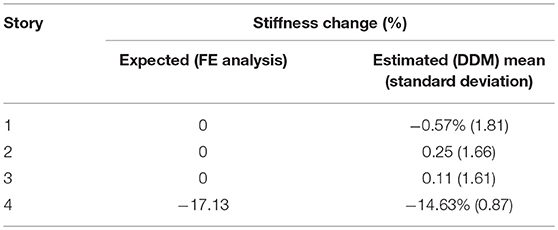
Table 4. Story stiffness change (DC S1).

The ARMAX analysis successfully located and quantified the damage in the fourth story while no substantial change was estimated in all other stories. The low standard deviation values for each story (average value of 1.49) illustrates the stability of the results through the 10 trials even with added noise.

Damage Case S2—Two Story Damage (1st and 2nd Stories)

The second damage case involved replacing two steel columns (A1 and B2 in Figure 5B) at the first story and one steel column (A1) at the second story with identically sized aluminum columns.

Similar to Damage Case S1, the damage ratios of the individual “damaged columns” is 0.685. SDF₁₁, which represents the change in stiffness of the combined first and second story was calculated as [((5 × 0) – (3 × 0.685))/8] = −25.69%. The change in stiffness of the second story, as shown in SDF₁₂ and SDF₂₁ was calculated as [((3 × 0) – (1 × 0.685))/4] = −17.13% and SDF₂₂ was calculated as [((7 × 0) – (1 × 0.315))/8] = −8.56%. For brevity, these calculations will not be shown for any further steel damage cases as the same process can be used for every damage case. In the results tables, each expected damage case result was completed by extracting the FE matrix, the hand calculations were only used as a second verification.

The overall change in stiffness at each story from both the expected results and the 5% noise ARMAX SDF are presented in Table 5 as per Equation (26).

TABLE 5

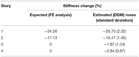
Table 5. Story stiffness change (DC S2).

The ARMAX DDM successfully located the damage on the first and second story while also measuring no substantial change in stiffness in the undamaged stories. The degree of damage on the first floor was underestimated by 4.81%, however the degree of damage on the second story was very close to the expected value. The low standard deviation values from the 10 trials illustrate the negligible impact that the 5% noise had on the ARMAX DDM.

Damage Case S3—Three Story Damage (1st, 2^nd, and 3rd Stories)

The final damage case for the experimental steel structure represents a more severe case in which there is damage on the first (A1, A2, and B1 in Figure 5B), second (B2) and third story (A1 and B1) with a total of six steel columns being replaced by aluminum columns. The overall stiffness loss values for each story are presented in Table 6.

TABLE 6

Table 6. Story stiffness change (DC S3).

The ARMAX DDM successfully located the damage at each story with excellent correlation to the expected degree of damage and relatively small differences between each trial.

The ARMAX analysis results from the numerical modeling produced results very similar to the results which were measured through previous tests on the experimental structure built by Do (2015). In each damage case, the ARMAX results successfully located and determined the degree of damage at each story without yielding significant false negative or positive results. In some cases, however, the ARMAX model underestimated the severity of damage to some extent.

Case Study II: 10 Story Concrete Structure

A 10 story structure with a 4 × 4 column layout as shown in Figure 7A was simulated. The 3D FE model as well as plan view of the model are presented in Figures 7B,C. Each column had identical rebar detailing and identical undamaged stiffness properties.

FIGURE 7

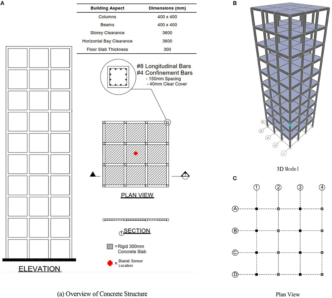
Figure 7. Overview and FE model for concrete structure. (A) Overview of concrete structure. (B) 3D model. (C) Plan view.

Damage Case C1—Two Story Damage (2nd and 5th Stories)

The first damage case incorporated moderate damage to eight columns; four columns (A2, B2, C2, and D2) with a DR of 0.50 and four columns (A4, B4, C4, and D4) with a DR of 0.55; at both the second and fifth story.

Equation (26) was used once again to calculate the story stiffness change at each level and the results are presented in Table 7 along with the standard deviation from the 10 trials.

TABLE 7

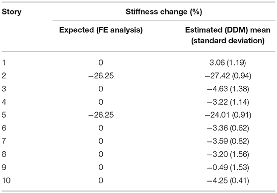
Table 7. Story stiffness change (DC C1).

The ARMAX DDM successfully located the damage in the second and fifth story. The severity of damage at each story was very close to the expected values with minimal standard deviations. Although there were some false positive SDF values that were higher than in the previous structures, it did not result in any issues as the highest false positive story stiffness change was calculated as −4.63%.

Damage Case C2—Five Story Damage (1st, 3rd, 4th, 7th, and 9th Stories)

The second damage case simulated a building which has undergone moderate to severe damage throughout with damage being applied to columns on five stories. The first story had five columns (A3, B2, B4, C4, and D2) damaged with DRs ranging from 0.50 to 0.65. The second story had five columns (A1, A2, B1, C3, and D3) damaged as well with two columns having a DR of 0.55 and three columns having a DR of 0.60. The fourth story incorporated damage in seven different columns (A2, A3, C1, C2, C3, and D4) with DRs ranging from 0.45 to 0.65. The seventh story had three columns (A3, B3, and B4) damaged: two with a DR of 0.55 and one with a DR of 0.50. The ninth story had four columns (B2, B3, C2, and C3) damaged, each with a DR of 0.40.

Similar to Damage Case C1, the noise continues to not have a major influence on the damage detection model. Table 8 presents the overall change in stiffness calculated at each story.

TABLE 8

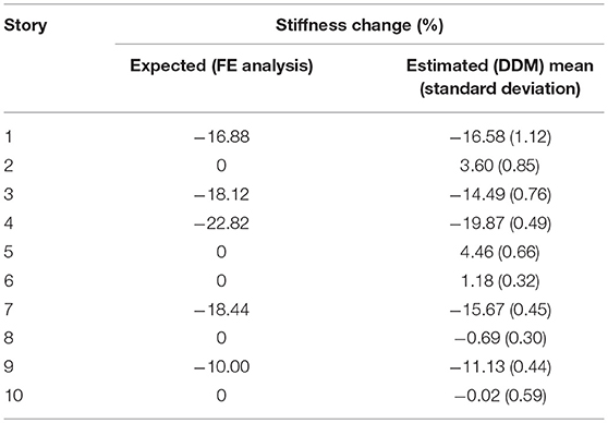
Table 8. Story stiffness change (DC C2).

The ARMAX DDM was successful in locating which five stories were damaged without calculating significant false negative or false positive results at the undamaged locations. Like the previous building model, the ARMAX DDM slightly underestimated the severity of damage when the number of damaged stories was increased.

Damage Case C3—Seven Story Damage (1st, 2nd, 3rd, 4th, 6th, 7th, and 8th Stories)

The final damage case tested represented a building that is in a critical state with damaged columns at seven different stories. The most severe damage was incorporated on the four lowest stories with the first, second, third, and fourth stories having ten (A1, B1, B3, B4, C1, C2, C3, C4, D2, and D4), nine (A1, A2, A4, B2, B3, C3, C4, D1, and D2), nine (A2, A3, B3, B4, C1, C2, C3, D3, and D4) and six (A3, A4, B2, B3, D1, and D2) columns damaged, respectively. The sixth, seventh and eighth stories each had seven columns damaged. To be more specific, the damaged columns for sixth story are at A2, A3, A4, B2, B3, C3, and C4. The damaged columns for seventh story are at A1, A2, A3, D1, D2, D3, and D4. The damaged columns for eighth story are at A2, A4, B3, B4, C1, C2, and C3.

The overall stiffness changes at each story are presented in Table 9.

TABLE 9

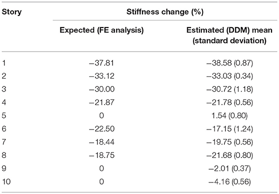
Table 9. Story stiffness change (DC C3).

The ARMAX DDM yielded excellent results by successfully locating the damage at each of the seven damaged stories. The degree of damage was calculated with excellent precision in the first four stories, however the model slightly underestimated the degree of damage in the three higher stories.

Discussion of Results

Overall, the ARMAX DDM was shown to effectively locate the damaged stories in both models with no significant errors. For most of the damage cases, the ARMAX DDM accurately estimated the degree of damage, however, the DDM had slightly less accurate results in the building model with more columns. This was expected, as the ARMAX DDM relies on approximating buildings as simplified shear type structures and ignoring the flexural deformation, so the ARMAX DDM generated nearly identical results to the FE models when the structures themselves were simplified. Through rigorous numerical testing, the ARMAX DDM was proven to be an effective and consistent method for locating and quantifying damage.

Conclusions and Future Work

In this paper, a new building damage detection model was proposed and developed using ARMAX analysis on the acceleration responses due to ambient wind loading. Through rigorous numerical modeling, it was demonstrated that damage can be identified at a story level precision and the degree of damage can be accurately quantified based on floor accelerations due to wind forces.

Within the detailed description of the methodology, the ARMAX model, used in conjunction with a sensor clustering concept to analyze the dynamic responses of a structure was explored. By assuming the mass of a building can be grouped into the floors and incorporating mathematical approximations, the ARMAX time series model was transformed to represent the general equation of motion. Using a sensor clustering technique, the ARMAX DDM was able to create a baseline case and damaged case of a structure and those two cases were then evaluated to create a stiffness damage feature capable of locating and quantifying damage at story level precision.

With an accurate account of the analysis model, forcing function and numerical damage model, the second part of the paper involved verifying the capability of the ARMAX DDM using numerical analysis. To illustrate the effectiveness, two separate building models were shown. The first was a previously built, experimental steel structure to which multiple impulse force loading was applied. The results from the ARMAX DDM effectively demonstrated that the parameters used in FE modeling accurately reflected real-life experimental behavior. The second structure was a 10 story reinforced concrete frame with a 4 × 4 column layout. Damage was successfully located and quantified in the minor, moderate and severe damage cases. Note, however, that the model slightly underestimated the degree of damage in some stories in the moderate and severe damage cases. The level of underestimation, however, was small enough to not warrant any major concerns. Overall, the ARMAX DDM was proven to be an effective and consistent method for locating and quantifying damage at a story level precision.

The ARMAX DDM has provided accurate results in multiple damage building scenarios, however there are still limitations that are worth mentioning and recommendations for future work. One limitation of this paper is that although it was validated through various numerical model testing, there have been no experimental structures tested using wind induced vibrations. The numerical damage detection model incorporated a uniform change in material properties in only the columns, with the rigid beams and slabs being unaffected. It is recommended that tests be done which may simulate more realistic structural damage. This may include incorporating severe material property changes in the tops and bottoms of the columns while not affecting the middle elevation as much. This could also include not treating the beams and slabs as rigid members and instead applying damage to them and including plastic hinge effects, i.e., not assuming the structure as shear type. Although the damage model was shown to be effective when replacing a steel column with an aluminum one, it is recommended that the ARMAX DDM be tested on a more realistic damage case for steel structures. It is also recommended that the timber buildings be tested. Further investigation should also be completed which look into adding 10% noise instead of the 5% used. In addition, as the dynamic system becomes faster in comparison to the sampling rate, the first order forward difference to approximate derivative may no longer be suitable, a higher order approximation or up-sampling techniques could be applied.

Author Contributions

GG used the ARMAX model for wind induced vibration, implemented the numerical analysis for verification and drafted the paper. QM developed part of the methodology and drafted the paper. MG is the supervisor of the other two authors who came up with the idea and concept, guided the direction of research, checked the proposed approach in this paper and revised the manuscript, and coordinated the funding for the project.

Funding

This research was partly supported by the Natural Sciences and Engineering Research Council of Canada through the Discovery Grants.

Conflict of Interest Statement

The authors declare that the research was conducted in the absence of any commercial or financial relationships that could be construed as a potential conflict of interest.

References

Bañuelos-Ruedas, F., Angeles-Camacho, C., and Rios-Marcuello, S. (2010). Analysis and validation of the methodology used in the extrapolation of wind speed data at different heights. Renew. Sustain. Energy Rev. 14, 2383–2391. doi: 10.1016/j.rser.2010.05.001

CrossRef Full Text | Google Scholar

Bao, C., Hao, H., and Li, Z. (2013). Integrated ARMA model method for damage detection of subsea pipeline system. Eng. Struct. 48, 176–192. doi: 10.1016/j.engstruct.2012.09.033

CrossRef Full Text | Google Scholar

Bayem, H., Phulpin, Y., Dessante, P., and Bect, J. (2008). “Probabilistic computation of wind farm power generation based on wind turbine dynamic modeling. Probabilistic Methods Applied to Power Systems, 2008,” in Proceedings of the 10th International Conference on PMAPS'08, eds P. Jirutitijaroen and C. Singh (Rincón).

Google Scholar

Bodeux, J.-B., and Golinval, J.-C. (2000). “ARMAV model technique for system identification and damage detection,” in Proceedings of the European COST F3 Conference on System Identification and Structural Health Monitoring, eds A. G. Gordo and J. A. Güemes (Madrid: Universidad Politécnica de Madrid), 303–312.

Google Scholar

Cement Association of Canada and Canadian Standards Association (2016). Concrete Design Handbook, 4th Edn. Ottawa, ON: Cement Association of Canada.

Chang, G. A., and Mander, J. B. (1994). Seismic Energy Based Fatigue Damage Analysis of Bridge Columns: Part I-Evaluation of Seismic Capacity. NCEER Technical Report No. NCEER-94-0006, State University of New York, Buffalo, NY.

Google Scholar

de Lautour, O., and Omenzetter, P. (2006). “Generalized seismic–induced structural damage prediction using artificial neural networks,” in 1st European Conference on Earthquake Engineering and Seismology (Geneva).

Google Scholar

Do, N. T. (2015). Detection of Stiffness and Mass Changes Separately Using Output-only Vibration Data. Edmonton, AB: University of Alberta.

Google Scholar

Fernandez, F., and Alonso, J. (2017). Wind speed generation for dynamic analysis. Wind Energy 20, 1049–1068. doi: 10.1002/we.2079

CrossRef Full Text | Google Scholar

Grosso, M. (1992). Wind pressure distribution around buildings: a parametrical model. Energy Build. 18, 101–131. doi: 10.1016/0378-7788(92)90041-E

CrossRef Full Text | Google Scholar

Gul, M., and Catbas, F. N. (2009). Statistical pattern recognition for structural health monitoring using time series modeling: theory and experimental verifications. Mech. Syst. Signal Process. 23, 2192–2204. doi: 10.1016/j.ymssp.2009.02.013

CrossRef Full Text | Google Scholar

Gul, M., and Catbas, F. N. (2011). Structural health monitoring and damage assessment using a novel time series analysis methodology with sensor clustering. J. Sound Vib. 330, 1196–1210. doi: 10.1016/j.jsv.2010.09.024

CrossRef Full Text | Google Scholar

Guo, Z., Zhang, Y., Lu, J., and Fan, J. (2016). Stiffness degradation-based damage model for RC members and structures using fiber-beam elements. Earthq. Eng. Eng. Vib. 15, 697–714. doi: 10.1007/s11803-016-0359-4

CrossRef Full Text | Google Scholar

Holmes, J. D. (2015). Wind Loading of Structures. Boca Raton, FL: CRC Press.

Google Scholar

Ji, X., Fenves, G. L., Kajiwara, K., and Nakashima, M. (2011). Seismic damage detection of a full-scale shaking table test structure. J. Struct. Eng. ASCE 137, 14–21. doi: 10.1061/(ASCE)ST.1943-541X.0000278

CrossRef Full Text | Google Scholar

Kim, Y. C., Kanda, J., and Yoon, S. W. (2009). Characteristics of longitudinal turbulence fluctuations in strong winds. Korea Soc. Steel Construct. 21, 40–45.

Google Scholar

Lakshmi, K., and Rama Mohan Rao, A. (2014). A robust damage-detection technique with environmental variability combining time-series models with principal components. Nondestruct. Test. Eval. 29, 357–376. doi: 10.1080/10589759.2014.949709

CrossRef Full Text | Google Scholar

Levy, H., and Lessman, F. (1961). Finite Difference Equations. New York, NY: The Macmillan Company.

Google Scholar

Lu, Y., and Gao, F. (2005). A novel time-domain auto-regressive model for structural damage diagnosis. J. Sound Vib. 283, 1031–1049. doi: 10.1016/j.jsv.2004.06.030

CrossRef Full Text | Google Scholar

Mei, Q., and Gül, M. (2014). Novel sensor clustering–based approach for simultaneous detection of stiffness and mass changes using output-only data. J. Struct. Eng. 141:04014237. doi: 10.1061/(ASCE)ST.1943-541X.0001218

CrossRef Full Text | Google Scholar

Mei, Q., and Gül, M. (2016). A fixed-order time series model for damage detection and localization. J. Civil Struct. Health Monitor. 6, 763–777. doi: 10.1007/s13349-016-0196-1

CrossRef Full Text | Google Scholar

Nair, K. K., Kiremidjian, A. S., and Law, K. H. (2006). Time series-based damage detection and localization algorithm with application to the ASCE benchmark structure. J. Sound Vib. 291, 349–368. doi: 10.1016/j.jsv.2005.06.016

CrossRef Full Text | Google Scholar

Newmark, N. M. (1982). Earthquake Spectra and Design. Berkeley, CA: Earthquake Eng. Research Institute.

Google Scholar

Nichita, C., Luca, D., Dakyo, B., and Ceanga, E. (2002). Large band simulation of the wind speed for real time wind turbine simulators. IEEE Trans. Energy Conv. 17, 523–529. doi: 10.1109/TEC.2002.805216

CrossRef Full Text | Google Scholar

Omenzetter, P., and Brownjohn, J. M. W. (2006). Application of time series analysis for bridge monitoring. Smart Mater. Struct. 15:129. doi: 10.1088/0964-1726/15/1/041

CrossRef Full Text | Google Scholar

Pearson, K. (1895). Note on regression and inheritance in the case of two parents. Proc. R. Soc. Lond. 58:240–242. doi: 10.1098/rspl.1895.0041

CrossRef Full Text | Google Scholar

Roy, K., Bhattacharya, B., and Ray-Chaudhuri, S. (2015). ARX model-based damage sensitive features for structural damage localization using output-only measurements. J. Sound Vib. 349, 99–102. doi: 10.1016/j.jsv.2015.03.038

CrossRef Full Text | Google Scholar

Rytter, A. (1993). Vibrational Based Inspection of Civil Engineering Structures. Aalborg: Dept. of Building Technology and Structural Engineering, Aalborg University.

Google Scholar

Sohn, H., and Farrar, C. R. (2001). Damage diagnosis using time series analysis of vibration signals. Smart Mater. Struct. 10:446. doi: 10.1088/0964-1726/10/3/304

CrossRef Full Text | Google Scholar

Sohn, H., Farrar, C. R., Hunter, N. F., and Worden, K. (2001). Structural health monitoring using statistical pattern recognition techniques. J. Dyn. Syst. Meas. Control 123, 706–711. doi: 10.1115/1.1410933

CrossRef Full Text | Google Scholar

Toussi, S., and Yao, J. T. (1983). Hysteresis identification of existing structures. J. Eng. Mech. 109, 1189–1202. doi: 10.1061/(ASCE)0733-9399(1983)109:5(1189)

CrossRef Full Text | Google Scholar

Welfonder, E., Neifer, R., and Spanner, M. (1997). Development and experimental identification of dynamic models for wind turbines. Control Eng. Pract. 5, 63–73. doi: 10.1016/S0967-0661(96)00208-0

CrossRef Full Text | Google Scholar