Simultaneous Approach to Critical Fault Rupture Slip Distribution and Optimal Damper Placement for Resilient Building Design

Introduction

It is well-accepted that earthquake ground motions exhibit diverse aspects, as observed, for example, in Mexico (1985), Northridge (1994), Kobe (1995), Chi-chi (1999), Tohoku (2011), Kumamoto (2016). Several models have been introduced to model these ground motions taking into account their occurrence mechanisms. Recently the main stream of investigations on the process of ground motion generation is composed of the following three components, (i) the fault rupture, (ii) the wave propagation to the earthquake bedrock, (iii) the site amplification to the ground surface. To include these modeling stages, four approaches have been developed in general, (a) the theoretical approach, (b) the numerical analysis approach, (c) the semi-empirical approach and (d) the hybrid approach. It is understood that, while the theoretical and numerical analysis approaches (finite difference method as a representative; see Day, 1982; Makita et al., 2019) are appropriate for producing directivity pulses and surface waves with the predominant period longer than 1–2 s (Bouchon, 1981; Hisada and Bielak, 2003; Yoshimura et al., 2003; Nickman et al., 2013), the semi-empirical approach is appropriate for ground motions with the predominant period shorter than 1–2 s. The empirical Green's function (Wennerberg, 1990) and the stochastic Green's function (Hisada, 2008) are frequently incorporated into the semi-empirical approach. In the hybrid approach, the shorter period ground motions are combined with the longer period waves through a matching filter.

Due to lack of sufficient observed data and intrinsic variability of characteristics in underground, it is usually recommended to treat several parameters as uncertain numbers (aleatory or epistemic) (Abrahamson et al., 1998; Lawrence Livermore National Laboratory, 2002; Morikawa et al., 2008; Cotton et al., 2013).

To investigate the effect of uncertainties in ground motions on structural response variability, Makita et al. (2018a) treated a base-isolated, building-connected hybrid structural system (Murase et al., 2013, 2014; Kasagi et al., 2016; Fukumoto and Takewaki, 2017) and tackled the effect of the uncertainty in site amplification. They dealt with the fault as a point source. On the other hand, the uncertainty in fault rupture slip is considered in the present paper and a recent one (Makita et al., 2018b). In modeling the wave propagation to the earthquake bedrock, the stochastic Green's function method is used (Irikura, 1986; Yokoi and Irikura, 1991). The Fourier amplitude of ground motions at the earthquake bedrock caused by rupture at a fault element is represented by the Boore's model (Boore, 1983) and the phase angle is represented by the phase difference method (Yamane and Nagahashi, 2008).

In this paper, the uncertainty in the fault rupture slip is taken as a main factor of uncertainty in the ground motion generation and the critical fault rupture slip distribution is found by using the stochastic Green's function method as a generator of ground motions. Then, a multi-degree-of-freedom (MDOF) building structure is introduced as a model structure and an optimal damper placement problem is discussed for the critical ground motion causing the maximum response (Drenick, 1970; Takewaki, 2007). The main topic in this paper is the simultaneous determination of the critical fault rupture slip distribution and the optimal damper placement (see Domenico et al., 2019 as a recent review paper). The sequential quadratic programming method is used in the problem of critical fault rupture slip distributions and a sensitivity-based method is introduced in the optimal damper placement problem. Furthermore, the robustness for the maximum interstory drift in MDOF building structures under the uncertainty in fault rupture slip distribution is presented for resilient building design by using the robustness function (Ben-Haim, 2006). Since the critical case leads to the most unfavorable structural response, the proposed method can provide structural designers with a promising tool for resilient building design.

Stochastic Green's Function Method for Ground Motion Generation

The present paper uses the stochastic Green's function method based on a plane-source model of the fault rupture to produce ground motions. Since the detailed explanation was provided in the reference (Makita et al., 2018b), a concise summary is presented in this section.

Generation of Ground Motion Using Small Ground Motions From Sub-fault Elements

The fault plane is divided into multiple fault elements and taking into account the delay of the fault element rupture initiation.

The fault plane is assumed to consist of N_L × N_W fault elements (N_L: number of divisions in the longitudinal direction, N_W: number of divisions in the width direction) and the slip action in one fault element is assumed to be composed of N_D slips. Due to Irikura (1983), the ground displacement U_ij(t) from one fault element is produced by N_D slips u_ij(t).

$\begin{array}{ll}{U}_{ij}(t)=f(t)*u_{ij}(t)={\displaystyle \sum _{k=1}^{N_D}}{u}_{ij}\left(t-\left(k-1\right)\frac{{\tau }_{ij}}{N_D}\right)& (1)\end{array}$

where ij refers to the ij sub-element in one fault element and τ_ij is the rise time of the ij sub-element. Let f(t) denote the slip correction function expressed by

$\begin{array}{ll}f(t)={\displaystyle \sum _{k=1}^{N_D}}\delta \left(t-\left(k-1\right)\frac{{\tau }_{ij}}{N_D}\right)& (2)\end{array}$

where δ(t) is the Dirac delta function.

The ground displacement U(t) resulting from the whole fault may then be given by

$\begin{array}{l}U\left(t\right)={\displaystyle \sum _{i=1}^{N_W}}{\displaystyle \sum _{j=1}^{N_L}}f\left(t-t_{ij}\right)*u_{ij}(t)\\ ={\displaystyle \sum _{i=1}^{N_W}}{\displaystyle \sum _{j=1}^{N_L}}{\displaystyle \sum _{k=1}^{N_D}}{u}_{ij}\left(t-t_{ij}-(k-1)\frac{{\tau }_{ij}}{N_D}\right)& (3)\end{array}$

In this paper, the following slip correction function f(t) is used (Irikura, 1986; Yokoi and Irikura, 1991).

$\begin{array}{ll}f(t)=\delta (t)+\frac{1}{n^{\prime }}{\displaystyle \sum _{k=1}^{(N_D-1)n^{\prime }}}{u}_{ij}\left(t-\frac{\left(k-1\right)\tau }{(N_D-1)n^{\prime }}\right)& (4)\end{array}$

The number n′ of re-division was introduced by Irikura (1986) to remove the effect of artificial periodicity. Irikura (1994) introduced the following constraint for n′.

$\begin{array}{ll}\frac{n^{\prime }{N}_D}{\tau }>2f_H(f_H:\text{ upper bound of the effective frequency})& (5)\end{array}$

The ground displacement U(t) resulting from the whole fault can finally be given by

$\begin{array}{l}U(t)={\displaystyle \sum _i^{N_L}}{\displaystyle \sum _j^{N_W}}{u}_{ij}\left(t-t_{ij}\right)\\ +{\displaystyle \sum _i^{N_L}}{\displaystyle \sum _j^{N_W}}{\displaystyle \sum _k^{(N_D-1)n^{\prime }}}\frac{1}{n^{\prime }}{u}_{ij}\left(t-t_{ij}-\frac{\left(k-1\right)\tau }{(N_D-1)n^{\prime }}\right)& (6)\end{array}$

The concept of the stochastic Green's function method used in the present study is illustrated in Figure 1A.

FIGURE 1

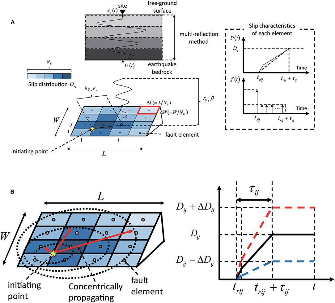
Figure 1. Ground motion generation method and fault slip model. (A) Concept of stochastic Green's function method used in the present paper. (B) Concentrically propagating slip model and uncertainty in slip quantity.

For simplicity, it is assumed here that the fault rupture propagates concentrically. t_ij can then be expressed by

$\begin{array}{ll}{t}_{ij}=t_{pij}+t_{rij}=\frac{r_{ij}}{\beta }+\frac{{\eta }_{ij}}{V_r}& (7)\end{array}$

where β: the shear wave velocity of the ground, V_r: the slip propagation speed in the fault, t_pij: the propagation time from the fault element to the recording point, t_rij: the slip initiation time in the fault element, r_ij: the distance between the fault element and the recording point, η_ij: the distance between the slip initiation point in the whole fault and the fault element.

In the present paper, it is assumed that the slip front parameters (slip initiation time t_rij and rise time τ_ij) are regarded as certain parameters and the fault slip distribution is treated as a set of uncertain parameters. The model is explained conceptually in Figure 1B.

Small Ground Motion From Element Fault

A small ground acceleration at the earthquake bedrock resulting from the slip of a fault element can be obtained by locating a point source at the center of the fault element (Boore, 1983). The Fourier amplitude spectrum of the acceleration at the earthquake bedrock can be given by

$\begin{array}{ll}\left|{F_{ij}}^S(\omega )\right|=S(\omega )·P(\omega )& (8)\end{array}$

where S(ω): parameter related to the source (fault), P(ω): parameter related to the wave attenuation in the wave passage from the fault element to the earthquake bedrock.

In this paper, S(ω) and P(ω) are from Boore (1983) (see Makita et al., 2018b). Since the phase is not given by Boore (1983), the phase difference method is introduced for expressing the phase of ground motion (Yamane and Nagahashi, 2008). The standard deviation of the phase difference resulting from the fault element ijcan be given by

$\begin{array}{ll}{\sigma }_{ij}/\pi =0.06+0.0003r_{ij}& (9)\end{array}$

This relation was derived for inland earthquakes (Makita et al., 2018a). The near-fault ground motion is assumed here in which the influence of the rupture directivity is small. In the case where the influence of the rupture directivity is not small, the relations σ_ij/π = 0.05 + 0.0003r_ij (in the direction of rupture propagation) and σ_ij/π = 0.08 + 0.0003r_ij(in the orthogonal direction of rupture propagation) are recommended (Yamane and Nagahashi, 2008). The phase spectrum is then expressed by

$\begin{array}{l}{\varphi }_{k+1ij}={\varphi }_{kij}+\Delta {\varphi }_{kij}(k=1,2,\dots ,N/2-1)\\ \Delta {\varphi }_{ij}=-(\mu +s·{\sigma }_{ij})& (10)\end{array}$

where ϕ_kij: the k-th phase spectrum of the fault element, Δϕ_kij: the k-th phase difference spectrum of the fault element ij, N: the number of adopted frequencies, μ: the mean phase difference, s: the Gaussian random number (mean = 0, standard deviation = 1). A constant value of μ is assumed here in all the fault elements.

The Fourier transform ${F_{ij}}^S(\omega )$ of the acceleration at the earthquake bedrock resulting from the fault element ij can be described by

$\begin{array}{ll}{F_{ij}}^S(\omega )=\left|{F_{ij}}^S(\omega )\right|·e^{i{\varphi }_{ij}(\omega )}& (11)\end{array}$

The inverse Fourier transform of ${F_{ij}}^S(\omega )$ provides the acceleration at the earthquake bedrock resulting from the fault element ij. The substitution of this into Equation (6) finally provides the acceleration at the earthquake bedrock resulting from the whole fault. It is noted that the difference of displacement and acceleration does not matter.

Critical Slip Distribution in Fault Plane Maximizing the Structural Response

The sequential quadratic programming method is used in the problem of critical fault rupture slip distributions maximizing the structural response.

Let x and f(x) denote the uncertain parameters (slip quantities of fault elements) and the maximum interstory drift with respect to the total duration of building response and all stories. The problem of critical fault slip distribution can be described as

$\begin{array}{ll}\text{Find}& \text{x}\\ \text{which maximizes}& f\text{(}\text{x}\text{)}\\ \text{subject to}& {\text{x}}_{lb}\le \text{x}\le {\text{x}}_{ub}& (12)\end{array}$

where x_lb and x_ub are the lower and upper bounds of uncertain parameters (slips).

In the present paper, viscous dampers are added in the building. Let c_di and ${\bar{W}}_c$ denote the viscous damping coefficient in the i-th story and the upper limit of the total quantity of damping coefficients. The problem of critical fault slip distribution for a building with added dampers can be described as

$\begin{array}{ll}\text{Find}& \text{x}\\ \text{which maximizes}& f\text{(}\text{x},{\text{c}}_d\text{)}\\ \text{subject to}& {\text{x}}_{lb}\le \text{x}\le {\text{x}}_{ub}\\ & {\displaystyle \sum _{i=1}^N}{c}_{di}\le {\bar{W}}_c,c_{di}\ge 0& (13)\end{array}$

A further criterion has to be introduced to determine the damper distribution. For this purpose, the following problem of minimizing the maximum interstory drift is posed.

$\begin{array}{ll}\text{Find}& \text{x},{\text{c}}_d\\ \text{which }{\displaystyle \underset{{\text{c}}_d}{\text{minimize}}}{\displaystyle \underset{\text{x}}{\text{ maximize}}}& f\text{(}\text{x},{\text{c}}_d\text{)}\\ \text{subject to}& {\text{x}}_{lb}\le \text{x}\le {\text{x}}_{ub}\\ & {\displaystyle \sum _{i=1}^N}{c}_{di}\le {\bar{W}}_c,c_{di}\ge 0& (14)\end{array}$

A solution procedure of this problem will be presented in the following section.

Simultaneous Determination of Critical Slip Distribution in Fault Plane and Optimal Damper Distribution

The solution procedure of the above final problem may be stated as follows:

① A model with uniform damper distribution for fixed total amount is defined as a “standard arrangement model,” and one without damper is set as an initial “adopted model”.

② Create “candidate models” of N patterns in which a small amount of damping coefficient is added to any one of the first to the Nth stories in the “adopted model” by using a sensitivity-based method.

③ Among the “candidate models,” the model with the smallest maximum interstory displacement is chosen as a new “adopted model” by using a sensitivity-based method.

④ Update the critical ground motion in every P step for damper arrangement by using the SQP method.

⑤ Define the final “adopted model” as the “optimal placement model”.

The flow chart and conceptual diagram are shown in Figure 2.

FIGURE 2

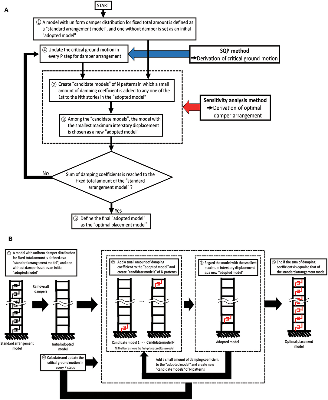
Figure 2. Simultaneous implementation of critical ground motion generation and optimal damper placement, (A) flow chart, (B) conceptual diagram.

Numerical examples

Fault Model, Soil Conditions, and Recording Points

The model S21 in the benchmark test by Kato et al. (2011) was used for verification of accuracy and reliability of the method for ground motion generation employed in the present paper. The result of the verification is shown in Makita et al. (2018b). While the benchmark test uses an empirical envelope function of acceleration time histories, the method used in Makita et al. (2018b) and this paper employs the phase difference method for expressing the phase. Since the same fault model is used in the present paper, the fault model, soil conditions, and recording points are explained here again.

The fault plane and three recording points used in the reference (Kato et al., 2011) are shown in Figure 3. The number of fault elements (N_L, N_W) follows (Kato et al., 2011). Several convergence investigations on the number of fault elements were done in the previous research (Irikura, 1994; Kato et al., 2011) together with the consideration of reasonable analysis time. The well-known scaling law (Irikura, 1983; Makita et al., 2018b) provides the suggestion on the selection of N_L, N_W, N_D. It seems interesting to investigate how the critical fault distribution can be affected by the number of fault elements. However, this requires further computation which cannot be achieved in the framework of the present paper. This investigation will be conducted in the future. The recording points are three points (a), (b), (c). The point (b) corresponds to the epicenter. It is assumed that the fault plane is vertical and the fault type is the right-lateral strike-slip fault. The detailed fault parameters are as follows: the fault length = 8,000 m, width = 4,000 m, slip = 1 m, seismic moment = $M_0=1.04\times {10}^{18}Nm$, strike, dip, and rake angles are θ = 90°, δ = 90°, and λ = 180°, respectively. The hypocenter is located at the point (0, 1,000 m, 4,000 m) and the fault rupture propagates concentrically with rupture velocity V_r = 3, 000 (m/s). The hypocenter of each sub-fault is assumed to be located at its center.

FIGURE 3

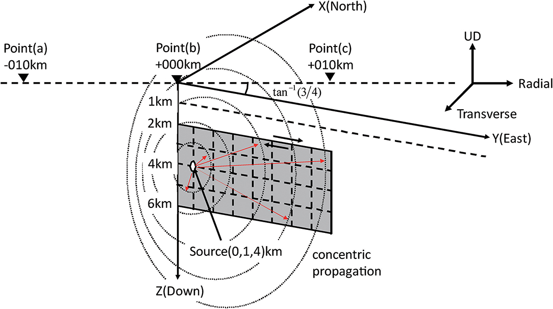
Figure 3. Fault plane and three recording points (replotted based on Kato et al., 2011).

Following the investigations by Somerville et al. (1999), Eshelby (1957), and Brune (1970), it is assumed that the stress drop Δσ of large earthquakes and the corner frequency f_c are given by the following equations:

$\begin{array}{ll}\Delta \sigma ={\displaystyle \frac{7}{16}}\frac{M_0}{R^3}\times {10}^{-14}& (15)\end{array}$

$\begin{array}{ll}{f}_c=4.9·{10}^6{V}_s{\left(\frac{\Delta \sigma }{M_0}\right)}^{1/3}& (16)\end{array}$

where R (km) is the effective radius of the fault (S = πR², S:fault area). In these equations, the unit of V_s is km/s, that of Δσ is bar and that of M₀ is dyne-cm.

From Equations (15), (16), Δσ = 13.95 (Mpa) and f_c = 0.404 (Hz) are derived. In this case, τ = 2/f_c ≈ 5.0 (s) is obtained from Boore (1983). The soil conditions are shown in Table 1A and the amplification of ground motion is described by one-dimensional wave propagation theory.

TABLE 1

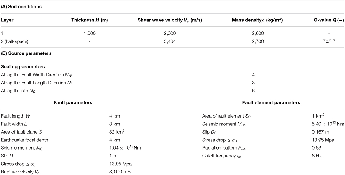
Table 1. Soil conditions and source parameters.

The division of the fault plane is N_W × N_L, i.e., N_W = 4: fault width direction and N_L = 8: fault length direction. The area of sub-fault is given by $S_S=1({\text{km}}^2)$. The seismic moment in each fault element (M_0S) is 5.40 × 10¹⁵Nm and the stress drop (Δσ_S) in each fault element is assumed to be 13.95 (Mpa). The slip D_S of each sub-fault is given by 0.167 (m) from M_0S = μS_SD_S and N_D = 6 from the ratio of fault plane to sub-fault (1 m/0.167 m). The seismic moment after superimposing the small earthquakes (${M_0}^{\prime }$) is calculated as ${M_0}^{\prime }=N_W·N_L·N_D·M_{0S}\approx 1.04\times {10}^{18}\mathrm{\text{(Nm)}}$, which is the same as M₀. The corner frequency f_cS = 2.33 Hz (Equation 16). As for the phase angle, the standard deviation of phase differences (σ_ij/π) are obtained from Equation (10) and its mean μ/π in each point is given by −0.140 at Point (a), −0.125 at Point (b) and −0.130 at Point (c). It is assumed that the horizontal component of superimposing wave is considered and only the SH wave is generated. Each small earthquake is produced by disassembling into the NS direction component and the EW direction component. Table 1B indicates the source parameters of the fault plane and sub-faults.

It seems interesting to investigate the relation between the number of slips N_D and the number of fault elements and the balance between the slips size and the elements size as well as between them and the slip initiation and rise times (Irikura, 1994; Kato et al., 2011). If necessary, the influence of the introduction of re-division of fault elements may be possible by using the condition on the expressibility of fault rupture processes (Irikura, 1994; Kato et al., 2011). However, these requires further computation which cannot be achieved in the framework of the present paper.

Setting of Uncertain Fault Slip Distribution

Let regard the fault slip distribution D as a set of uncertain parameters. If the nominal value of D, the base quantities of variation of D (toward decreasing side and increasing side) and the degree of variability are denoted by ${D_{ij}}^C$, $\Delta {\underset{-}{D}}_{ij}$, $\Delta {\bar{D}}_{ij}$, and α, the interval parameter expression can be given by

$\begin{array}{l}{\text{D}}^I=\left\{\left[{D_{ij}}^C-\alpha \Delta {{\displaystyle \underset{-}{D}}}_{ij},{D_{ij}}^C+\alpha \Delta {\bar{D}}_{ij}\right]\right\}\\ (i=1,\cdots NW,j=1,\cdots NL)& (17)\end{array}$

In this paper, α = 0.3, $\Delta {\underset{-}{D}}_{ij}=\Delta {\bar{D}}_{ij}={D_{ij}}^C$ are given.

Setting of Building Structures

A shear-type building structure is employed as the super building model. 2-, 5-, 10-, and 20-story buildings are considered. The floor mass, fundamental natural period, structural damping ratio and total added damping coefficient are shown in Table 2. The total damping coefficient corresponds approximately to the damping ratio 0.2. Three story stiffness distributions are treated, i.e., model with straight lowest natural mode, model with trapezoidal stiffness distribution, model with uniform stiffness distribution. These story stiffness distributions are shown in Figure 4.

TABLE 2

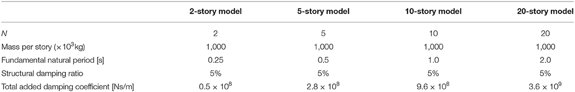
Table 2. Parameters in building structures.

FIGURE 4

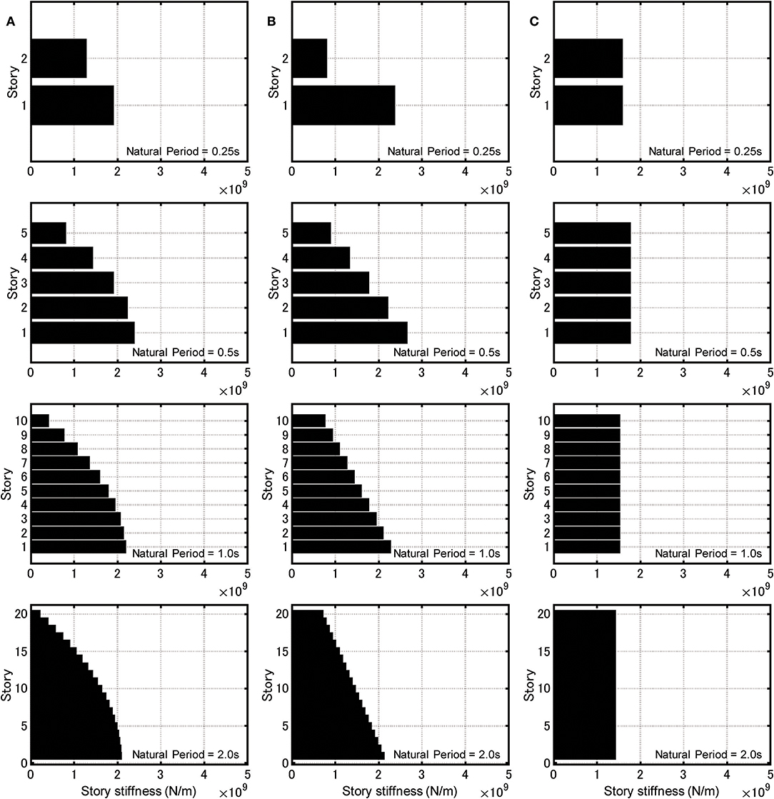
Figure 4. Story stiffness distributions of three building structures. (A) Model with straight lowest natural mode. (B) Model with trapezoidal stiffness distribution. (C) Model with uniform stiffness distribution.

Computational Time Saving by Skipping the Procedure for Updating Critical Fault Slip Distribution and Its Accuracy Verification

The sequential quadratic programming method for the problem of critical fault slip and the sensitivity-based method for the problem of optimal damper placement are time-consuming. Especially, the sequential quadratic programming method for the problem of critical fault slip needs a lot of computational time. Therefore, a method for reducing the computational load is desired. For this purpose, a method of skipping some steps for updating the critical fault slip in simultaneous analysis of critical fault slip and optimal damper placement is proposed here which was explained in Figure 2.

Figure 5 shows the influence of number of skipped steps on the results of the 10-story MDOF model with straight lowest natural mode. Figure 5A indicates accelerations of ground motions for four numbers of skipped steps (1, 5, 10, 20) and Figure 5B presents the maximum interstory drift. In these figures, the nominal case and critical case are treated. In Figure 5B, both the model with damping and the model without damping are investigated. It can be observed that no obvious difference can be seen in case that the number of skipped steps is smaller than 20. This means that the number of skipped steps smaller than 20 can save the computational time without deterioration of accuracy.

FIGURE 5

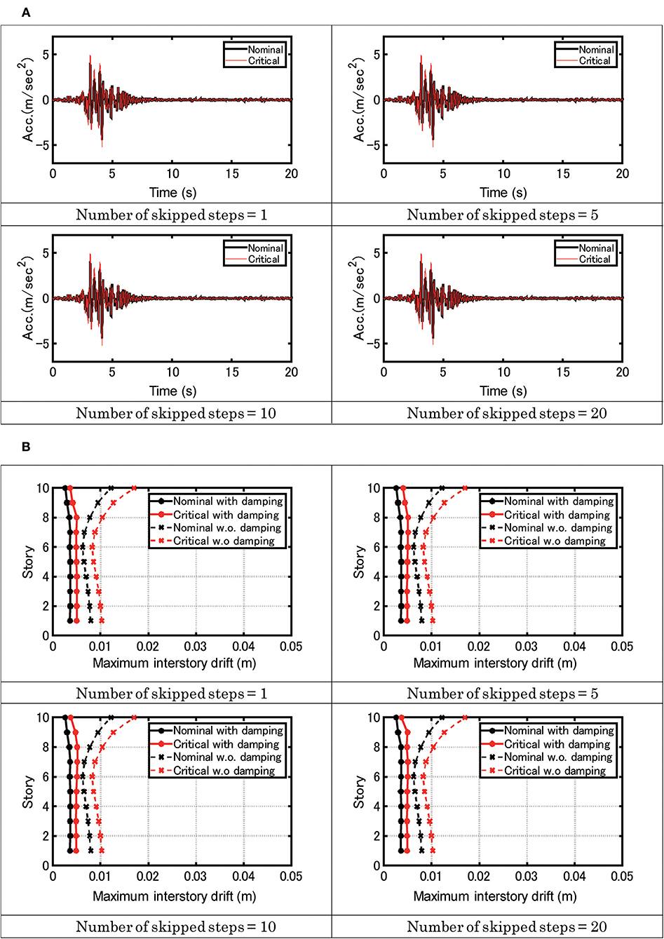
Figure 5. Influence of number of skipped steps. (A) Acceleration of ground motions for four numbers of skipped steps. (B) Maximum interstory drift of MDOF model for four numbers of skipped steps.

Figure 6 shows the computational analysis time for four numbers of skipped steps. The computer system is CPU: Core i5-6500 (3.2 GHz), RAM: 32.0 GB (DDR4-2132), OS: Windows 10 Pro (64 bit). It can be found that remarkable reduction of analysis time is possible by skipping some steps for updating the critical fault slip. For example, in the case where the fault rupture distribution is fixed (uncertainty level α = 0 in the robustness function analysis explained later), the computational time only for optimization with respect to viscous damper distribution is 3 min. This is 1/14 of the overall computational time (43 min in Figure 6 for 20 skipped steps) including the robustness function analysis (α = 0, 0.1, 0.2, 0.3).

FIGURE 6

Figure 6. Computational analysis time for four numbers of skipped steps.

Analysis Results

Figure 7 shows the nominal and critical ground surface accelerations of four MDOF models with different number of stories, 2, 5, 10, 20 [fundamental natural period, T₁ = 0.25, 0.5, 1.0, 2.0 (s)] at three points (a), (b), (c) (stiffness distribution: Straight lowest natural mode). It can be observed that the ground motion accelerations corresponding to the critical case are larger than those corresponding to the nominal case. The same observation was found for other models (trapezoidal stiffness distribution, uniform stiffness distribution).

FIGURE 7

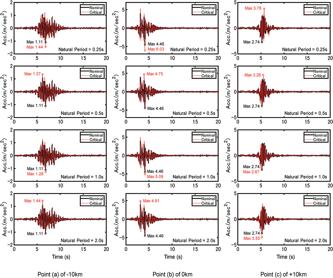
Figure 7. Nominal and critical ground surface accelerations of four MDOF models with different number of stories (T₁ = 0.25s, 0.5s, 1.0s, 2.0s) at three points (Straight lowest natural mode).

Figure 8 presents the Fourier amplitude spectra of nominal and critical ground surface accelerations of four MDOF models with different number of stories, 2, 5, 10, 20 [T₁ = 0.25, 0.5, 1.0, 2.0 (s)] at three points (Straight lowest natural mode). It can also be observed that the Fourier amplitudes of ground motion accelerations corresponding to the critical case are larger than those corresponding to the nominal case.

FIGURE 8

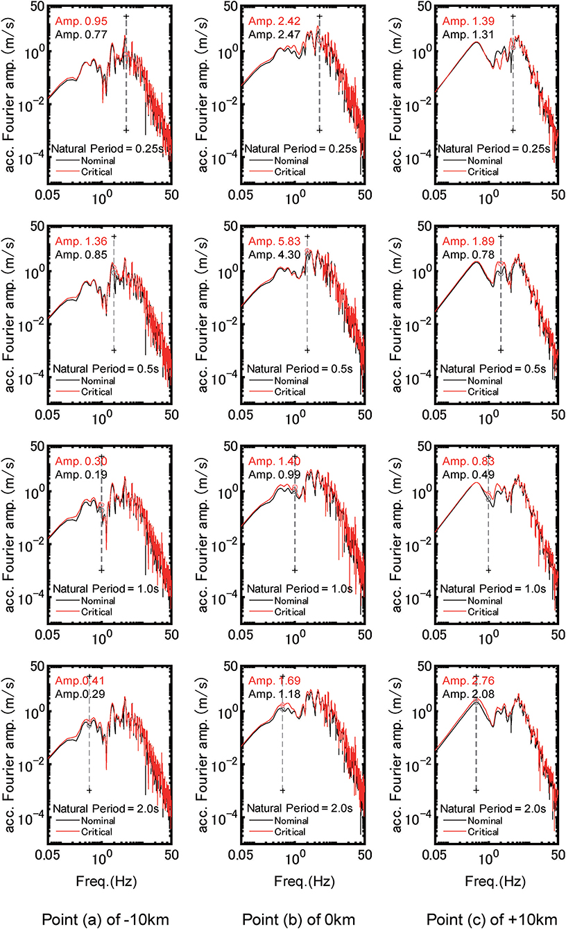
Figure 8. Fourier amplitude spectra of nominal and critical ground surface accelerations of four MDOF models with different number of stories (T₁ = 0.25s, 0.5s, 1.0s, 2.0s) at three points (Straight lowest natural mode).

Figure 9 indicates the nominal and critical maximum interstory drift distributions of four MDOF models with different number of stories, 2, 5, 10, 20 [T₁ = 0.25, 0.5, 1.0, 2.0 (s)] at three points (Straight lowest natural mode). For comparison, the cases without damper and with damper are shown. It can be found that the viscous dampers are extremely effective for the response reduction and the larger maximum interstory drifts in upper stories are well-reduced by the effect of viscous dampers. The structural response (interstory drift) at the point (b) (above the fault plane) is the maximum with an exception. Therefore, the optimal damper distribution for the point (b) is recommended only from the present result. Of course, when this distribution is adopted for other points (a), (c), the responses will become larger than those obtained for the model with the respective optimal damper distribution. On the other hand, if the optimal damper distribution adopted for the point (a) or (c) is used for the model at the point (b), the maximum interstory drift becomes larger than that evaluated for the optimal damper distribution determined for the point (b). This indicates the preference of selection of the optimal damper distribution at the point (b). Further investigation will be necessary to search the best damper distribution for guaranteeing the response constraints at all the points.

FIGURE 9

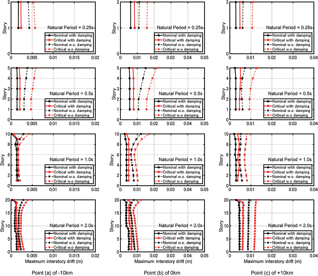
Figure 9. Nominal and critical maximum interstory drift distributions of four MDOF models with different number of stories (T₁ = 0.25s, 0.5s, 1.0s, 2.0s) at three points (Straight lowest natural mode).

Figure 10 shows the critical fault slip distribution of four MDOF models with different number of stories, 2, 5, 10, 20 [T₁ = 0.25, 0.5, 1.0, 2.0 (s)] at three points (Straight lowest natural mode). It can be understood that, in the critical case, the large slips are concentrated to the upper side of the fault plane which is near to the recording point.

FIGURE 10

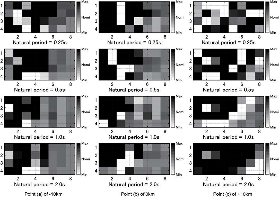
Figure 10. Critical fault slip distribution of four MDOF models with different number of stories (T₁ = 0.25s, 0.5s, 1.0s, 2.0s) at three points (Straight lowest natural mode).

Figure 11A presents the critical damping coefficient distributions of four MDOF models with different number of stories, 2, 5, 10, 20 [T₁ = 0.25, 0.5, 1.0, 2.0 (s)] at three points (Building model: Straight lowest natural mode). Similarly, Figure 11B indicates those for the building model with trapezoidal stiffness distribution and Figure 11C shows those for the building model with uniform stiffness distribution. It can be found that the damping coefficients are generally concentrated to the stories exhibiting larger maximum interstory drifts, i.e., the upper part for the model with straight lowest natural mode, the middle part for the model with trapezoidal stiffness distribution, the lower part for the model with uniform stiffness distribution. However, some exceptions exist in 2-story models. Because of the space problem (number of figures), the distribution of the maximum interstory drifts is shown in Figure 9 only for the model with straight lowest natural mode. However, the distribution of the maximum interstory drifts has been derived also for the models with trapezoidal stiffness distribution and with uniform stiffness distribution. These distributions demonstrate the conclusion derived just above.

FIGURE 11

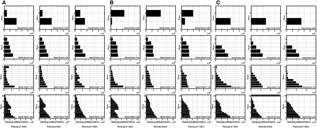
Figure 11. Critical damping coefficient distributions of four MDOF models with different number of stories (T₁ = 0.25s, 0.5s, 1.0s, 2.0s) at three points. (A) Model with straight lowest natural mode. (B) Model with trapezoidal stiffness distribution. (C) Model with uniform stiffness distribution.

Robustness Evaluation for Uncertain Fault Slip Distribution Using Robustness Function

To evaluate the robustness of building structures for uncertain fault slip distribution, the robustness function proposed by Ben-Haim (2006) is used. Let f_c, x^I, x(α) denote the specified limit value of the maximum interstory drift, the interval parameters (fault slip distribution D) and the admissible fault slip distribution for a specified uncertainty level α. x(α) is defined in Equation (17). The robustness function can be expressed by

$\begin{array}{ll}\widehat{\alpha }(\overline{x},f_c)=\max \left\{\alpha |\max \left\{f(x^I)|x^I\in x(\alpha )\right\}<f_c\right\}& (18)\end{array}$

where over-bar denotes the nominal parameter. The conceptual diagram of the robustness function $\widehat{\alpha }$ for various uncertainty levels is shown in Figure 12.

FIGURE 12

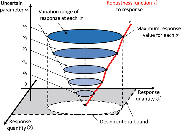
Figure 12. Robustness function $\widehat{\alpha }$ for various uncertainty levels.

Figure 13A shows the robustness function $\widehat{\alpha }$ with respect to the maximum interstory drift of the MDOF model with straight lowest natural mode for uncertain fault slip. These figures show the results for three recording points (a), (b), (c). Once the value $\widehat{\alpha }$ in the vertical axis is fixed, the corresponding maximum interstory drift of the MDOF model in the horizontal axis indicates the maximum value for varied possible uncertain parameters (quantity of fault rupture slip) prescribed by $\widehat{\alpha }$. It can be observed that the robustness becomes the smallest for the model at Point (b) (epicenter). This is because the response of the MDOF model is the largest at Point (b). The slope of the robustness function indicates the degree of the robustness. As the slope becomes steeper, the model becomes more robust (this indicates that the structural response is insensitive to change of fault rupture slip).

FIGURE 13

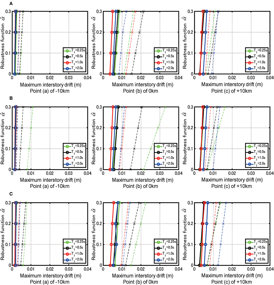
Figure 13. Robustness function $\widehat{\alpha }$ with respect to the maximum interstory drift of four MDOF models with different numbers of stories (T₁ = 0.25s, 0.5s, 1.0s, 2.0s) at three points. (A) Model with straight lowest natural mode. (B) Model with trapezoidal stiffness distribution. (C) Model with uniform stiffness distribution (solid line: with damper, broken line: without damper).

Figure 13B presents similar ones for the model with trapezoidal stiffness distribution and Figure 13C indicates those for the model with uniform stiffness distribution.

Since the robustness is closely related to the resilience, the presented method using the robustness function seems useful for the evaluation of resilience of buildings against uncertain fault slip distribution.

Conclusions

The uncertainty in the fault rupture slip was taken as a main source of uncertainty in the present paper and the critical fault rupture slip distribution producing the maximum structural response was found by using the stochastic Green's function method as a generator of ground motions. A multi-degree-of-freedom (MDOF) building structure was introduced as a model structure and an optimal damper placement problem was investigated for the critical ground motion. The main feature of this paper is the simultaneous treatment of the critical fault rupture slip distribution problem and the optimal damper placement problem. The sequential quadratic programming method was used in the problem of critical fault rupture slip distributions and a sensitivity-based method was introduced in the optimal damper placement problem. The robustness for the maximum interstory drift in MDOF building structures under the uncertainty in fault rupture slip distributions was presented for resilient building design by using the robustness function. The main results obtained in this paper may be summarized as follows.

(1) The ground motion accelerations corresponding to the critical case are larger than those corresponding to the nominal case. This can also be confirmed from the Fourier amplitudes of ground motion accelerations.

(2) In the critical case, the large slips are concentrated to the upper side of the fault plane which is near to the recording point.

(3) The ground surface acceleration at the epicenter becomes larger than that at other recording point. The maximum interstory drift of the super building at the epicenter also exhibits the largest value.

(4) Since the sequential quadratic programming method for the problem of critical fault slip and the sensitivity-based method for the problem of optimal damper placement are time-consuming, update of the critical fault slip distribution in each step of optimal damper placement may be unreasonable. Remarkable reduction of analysis time is possible by skipping some steps for updating the critical fault slip distribution.

(5) The viscous dampers are extremely effective for the response reduction and the larger maximum interstory drifts in upper stories are well-reduced by the effect of viscous dampers. The optimal damper distribution exhibits different properties depending on the stiffness distribution of super buildings. Large damper quantities are allocated to the stories exhibiting large interstory drifts, although some exceptions exist in two-story models. However, the point, at which the building is set, does not affect so much the optimal damper distribution.

(6) From the relation of the robustness function with the maximum interstory drift, the designers can find the level of potential robustness with respect to uncertain parameters for a specified level of the maximum interstory drift.

Even in the case where linear viscous dampers are used, the simultaneous extremization with respect to fault rupture distribution and viscous damper distribution requires many computational cycles and time. Therefore, the extension to non-linear viscous dampers appears to be the next step of research.

Data Availability Statement

All datasets generated for this study are included in the manuscript/supplementary files.

Author Contributions

KK formulated the problem, conducted the computation, and wrote the paper. IT supervised the research and wrote the paper.

Funding

Part of the present work was supported by KAKENHI of Japan Society for the Promotion of Science (Nos. 17K18922, 18H01584). This support was greatly appreciated.

Conflict of Interest

The authors declare that the research was conducted in the absence of any commercial or financial relationships that could be construed as a potential conflict of interest.

The reviewer DD declared a past co-authorship with one of the authors IT to the handling editor.

References

Abrahamson, N., Ashford, S., Elgamal, A., Kramer, S., Seible, F., and Somerville, P. (1998). Proceedings of the 1st PEER Workshop on Characterization of Special Source Effects (San Diego, CA: Pacific Earthquake Engineering Research Center, University of California).

Ben-Haim, Y. (2006). Info-Gap Decision Theory: Decisions Under Severe Uncertainty, 2nd Edn. London: Academic Press.

Google Scholar

Boore, D. M. (1983). Stochastic simulation of high-frequency ground motions based on seismological models of the radiated spectra. Bull. Seism. Soc. Am. 73, 1865–1894.

Google Scholar

Bouchon, M. (1981). A simple method to calculate Green's functions for elastic layered media. Bull. Seism. Soc. Am. 71, 959–971.

Brune, J. N. (1970). Tectonic stress and the spectra of seismic shear waves from earthquakes. J. Geophys. Res. 75, 4997–5009. doi: 10.1029/JB075i026p04997

CrossRef Full Text | Google Scholar

Cotton, F., Archuleta, R., and Causse, M. (2013). What is sigma of the stress drop? Seism. Res. Lett. 84, 42–48. doi: 10.1785/0220120087

CrossRef Full Text | Google Scholar

Day, S. M. (1982). Three-dimensional finite difference simulation of fault dynamics: rectangular fault with fixed rupture velocity. Bull. Seism. Soc. Am. 72, 83–96.

Google Scholar

Domenico, D. D., Ricciardi, G., and Takewaki, I. (2019). Design strategies of viscous dampers for seismic protection of building structures: a review. Soil Dyn. Earthquake Eng. 118, 144–165. doi: 10.1016/j.soildyn.2018.12.024

CrossRef Full Text | Google Scholar

Drenick, R. F. (1970). Model-free design of aseismic structures. J. Eng. Mech. Div. ASCE 96, 483–493.

Google Scholar

Eshelby, J. D. (1957). The determination of the elastic field of an ellipsoidal inclusion and related problems. Proc. R. Soc. A 241, 376–396. doi: 10.1098/rspa.1957.0133

CrossRef Full Text | Google Scholar

Fukumoto, Y., and Takewaki, I. (2017). Dual control high-rise building for robuster earthquake performance. Front. Built Environ. 3:12. doi: 10.3389/fbuil.2017.00012

CrossRef Full Text | Google Scholar

Hisada, Y. (2008). Broadband strong motion simulation in layered half-space using stochastic Green's function technique. J. Seismol. 12, 265–279. doi: 10.1007/s10950-008-9090-6

CrossRef Full Text | Google Scholar

Hisada, Y., and Bielak, J. (2003). A theoretical method for computing near-fault ground motions in layered half-spaces considering static offset due to surface faulting with a physical interpretation of fling step and rupture directivity. Bull. Seism. Soc. Am. 93, 1154–1168. doi: 10.1785/0120020165

CrossRef Full Text | Google Scholar

Irikura, K. (1983). Semi-empirical estimation of strong ground motions during large earthquakes. Bull. Disast. Prev. Res. Inst. Kyoto Univ. 33, 63–104.

Google Scholar

Irikura, K. (1986). “Prediction of strong acceleration motions using empirical Green's function,” in Proceedings of the 7th Japan Earthquake Engineering Symposium (Tokyo), 151–156.

Irikura, K. (1994). Earthquake source modeling for strong motion prediction. J. Seism. Soc. Jap. Second Ser. 46, 495–512. doi: 10.4294/zisin1948.46.4_495

CrossRef Full Text

Kasagi, M., Fujita, K., Tsuji, M., and Takewaki, I. (2016). Automatic generation of smart earthquake-resistant building system: hybrid system of base-isolation and building-connection. Heliyon 2:2. doi: 10.1016/j.heliyon.2016.e00069

PubMed Abstract | CrossRef Full Text | Google Scholar

Kato, K., Hisada, Y., Kawabe, H., Ohno, S., Nozu, A., Nobata, A., et al. (2011). Benchmark tests for strong ground motion prediction methods: case for stochastic Green's function method (Part1). J. Technol. Design 17, 49–54. doi: 10.3130/aijt.17.49

CrossRef Full Text

Lawrence Livermore National Laboratory (2002). Guidance for performing Probabilistic Seismic Hazard Analysis for a Nuclear Plant Site: Example Application to the Southeastern United States. NUREG/CR-6607, UCRL-ID-133494.

Makita, K., Kondo, K., and Takewaki, I. (2018b). Critical ground motion for resilient building design considering uncertainty of fault rupture slip. Front. Built Environ. 4:64. doi: 10.3389/fbuil.2018.00064

CrossRef Full Text | Google Scholar

Makita, K., Kondo, K., and Takewaki, I. (2019). Finite difference method-based critical ground motion and robustness evaluation for long-period building structures under uncertainty in fault rupture. Front. Built Environ. 5:2. doi: 10.3389/fbuil.2019.00002

CrossRef Full Text | Google Scholar

Makita, K., Murase, M., Kondo, K., and Takewaki, I. (2018a). Robustness evaluation of base-isolation building-connection hybrid controlled building structures considering uncertainties in deep ground. Front. Built Environ. 4:16. doi: 10.3389/fbuil.2018.00016

CrossRef Full Text | Google Scholar

Morikawa, N., Kanno, T., Narita, A., Fujiwara, H., Okumura, T., Fukushima, Y., et al. (2008). Strong motion uncertainty determined from observed records by dense network in Japan. J. Seismol. 12, 529–546. doi: 10.1007/s10950-008-9106-2

CrossRef Full Text | Google Scholar

Murase, M., Tsuji, M., and Takewaki, I. (2013). Smart passive control of buildings with higher redundancy and robustness using base-isolation and inter-connection. Earthquakes Struct. 4, 649–670. doi: 10.12989/eas.2013.4.6.649

CrossRef Full Text | Google Scholar

Murase, M., Tsuji, M., and Takewaki, I. (2014). Hybrid system of base isolation and building connection for control robust for broad type of earthquake ground motions. J. Struct. Eng. 60B, 413–422.

Nickman, A., Hosseini, A., Hamidi, J. H., and Barkhordari, M. A. (2013). Reproducing fling-step and forward directivity at near source site using of multi-objective particle swarm optimization and multi taper. Earthquake Eng. Eng. Vibration 12, 529–540. doi: 10.1007/s11803-013-0194-9

CrossRef Full Text | Google Scholar

Somerville, P., Irikura, K., Graves, R., Sawada, S., Wald, D., Anderson, N., et al. (1999). Characterizing crustal earthquake slip models for the prediction of strong ground motion. Seism. Res. Lett. 70, 59–80. doi: 10.1785/gssrl.70.1.59

CrossRef Full Text | Google Scholar

Takewaki, I. (2007). Critical Excitation Methods in Earthquake Engineering, 2nd edition. London: Elsevier.

Google Scholar

Wennerberg, L. (1990). Stochastic summation of empirical Green's functions. Bull. Seism. Soc. Am. 80, 1418–1432.

Google Scholar

Yamane, T., and Nagahashi, S. (2008). “A generation method of simulated earthquake ground motion considering phase difference characteristics,” in Proceedings of the 14th World Conference on Earthquake Engineering (Beijing).

Google Scholar

Yokoi, T., and Irikura, K. (1991). Empirical green's function technique based on the scaling law of source spectra. J. Seism. Soc. Jap. Second Ser. 44, 109–122. doi: 10.4294/zisin1948.44.2_109

CrossRef Full Text | Google Scholar

Yoshimura, C., Bielak, J., Hisada, Y., and Fernandez, A. (2003). Domain reduction method for three-dimensional earthquake modeling in localized regions, part II: verification and applications. Bull. Seism. Soc. Am. 93, 825–840. doi: 10.1785/0120010252

CrossRef Full Text | Google Scholar