Selecting and Scaling of Energy-Compatible Ground Motion Records

Introduction

The response history analysis for the seismic design and the evaluation of the performance of structures has evolved along with the rapid increase in the computational power of the various engineering software. This has enabled not only the application of a faster and more accurate linear elastic time history analysis of structures having some thousands degrees of freedom, but also of the nonlinear time history response analysis which is becoming more and more common nowadays. Traditionally, the seismic design of structures is based on a force-based and/or displacement based approach, in which the effect of the earthquake loading is quantified using the peak ground and response spectra acceleration of the corresponding ground motion record. However, the current status of the various norms regarding the selection of suitable ground motion records that meet specific requirements is rather simplified, which, despite the robustness of the various finite element models available for seismic design, may account for significant source of error in structural design. Therefore, the selection of appropriate sets of ground motion records for linear/nonlinear dynamic analysis of structures remains a challenge.

Although, large ground motion databases are today widely available, in engineering practice, the problem of record selection is tackled either through scaling a real ground motion, or generating them artificially. A state-of-the-art review on the available methods for selection and scaling of ground motion records is presented by Katsanos et al. (2010), whereas some critical issues in record selection and manipulation are presented by Iervolino et al. (2008). In case of limited availability of appropriate real acceleration time-histories, simulated strong motion records can be used (Boore, 2009; Graves and Pitarka, 2010). The generation of artificial/simulated spectrum-compatible ground motion records has some disadvantages against real ground motions. Artificial records have generally a large number of cycles of strong motion, which leads to increased energy content compared to real ground motions. Adjusting the Fourier spectrum of a real ground motion in the frequency domain with a view to matching a target spectrum at specific frequencies affects amplitude, frequency content and phasing, which generally tends to increase the total input energy. The same deficiencies are observed also in the simulated records, which may not produce similar nonlinear response in structures as real records due to unrealistic phasing as well as peaks and troughs effects (Atkinson and Goda, 2010).

An alternative formulation of the loading effect of earthquakes on structures can be based on the earthquake input energy, which is the internal product of force and displacement. Energy considerations for the seismic design of structures constitutes the basis of the energy-based seismic design (EBSD) approach and is gaining extensive attention (Uang and Bertero, 1988; Chou and Uang, 2003; Surahman, 2007; Leelataviwat et al., 2009; Jiao et al., 2011; López Almansa et al., 2013). Since in the EBSD methods the energy-absorption capacity of the structure and the input energy that comes from the ground motion are compared for seismic design, it is imperative to develop and use design energy input spectra (DEIS).

EBSD has many benefits and compensates the deficiencies related to the use of conventional acceleration or pseudo-acceleration response spectra as follows: (a) It accounts for the effects of duration of the cyclic loading of the earthquake ground motion. Therefore, it can adequately capture the different type of time histories (impulsive, non-impulsive, periodic with long-duration pulses, etc.) regarding their destructive potential. (b) It enables the quantitative evaluation of the cumulative structural damage in terms of hysteretic energy without the need to use equivalent viscous damping and/or ductility reduction. (c) There is no interdependence between the earthquake input energy and the structural resistance in terms of energy dissipation capacity. (d) The input energy that a structure experiences during an earthquake is governed primarily by its eigenperiod and mass and less by its strength or damping, except for the short-period range (Zahrah and Hall, 1984; Akiyama, 1985; Kuwamura and Galambos, 1989). This has been verified experimentally by Tselentis et al. (2010). Therefore, the input energy is a stable quantity that does not depend on many factors and thus is simpler to handle and interpret.

Given the advantages of the EBSD over the traditional approaches, the incorporation of not only acceleration spectra but also energy-based spectra for the generation of artificial ground motion records is an interesting alternative that could lead to more realistic spectrum-compatible design records (Chapman, 1999; Tselentis et al., 2010). Actually, it has been demonstrated that if the hazard is assessed on the basis of the earthquake input energy, the hazard posed by larger magnitude earthquakes contributes more to the total seismic hazard at a specific site, than that based on spectral acceleration (Tselentis et al., 2010). It is noted that the input energy spectrum that is obtained elastically is valid also for inelastic systems since the strength and plastification of the structure do not practically affect the total energy input (López Almansa et al., 2013; Dindar et al., 2015).

In this study a novel spectra-matching framework is developed, to generate artificial acceleration time histories perfectly matched a target spectrum. Apart from the well-known design acceleration spectrum that is prescribed by the various norms and guidelines, the seismic input energy equivalent velocity spectrum is also taken into account. This consideration is leading therefore to optimum acceleration time histories which represent actual motions in a much more realistic way. In order to produce elastic spectra that match as closely as possible to a given target spectrum, the procedure of selection and scaling of the suite of ground motion records to fit a given target spectrum is formulated as an optimization problem. Three characteristic ground motion records of different inherent nature are selected as target spectra, to verify the effectiveness of the proposed algorithm, ensuring that its performance is target spectrum independent assuming different matching scenarios. The optimization results have shown that there exists a good agreement between the target and optimum spectra for each case examined, regardless of the nature of target spectrum, demonstrating the reliability and performance of the proposed methodology.

Numerical Modeling

The main goal of this study is to obtain artificial ground motion records by performing as minimum as possible number of operations on the raw ground motion data. These ground motion records are linearly combined together forming a suite of records. The procedure of selection and scaling of the suite of ground motion records to fit a given target spectrum is formulated as an optimization problem. In this section, the process of the raw ground motion data as well as the ingredients for the formulation of the optimization problem are presented.

Processing Raw Ground Motion Data

A linear combination of real accelerograms requires only selection and scaling of the latter and does not alter their inherent characteristics (e.g., non-stationarity, coda, phase content, etc.), which have to be preserved in order to obtain realistic artificial records as a result of the linear combination. Since the real records have various durations, linear combination cannot be applied directly to the acceleration time histories. However, it can be applied to their Fourier spectra in the frequency domain which have the same length for all motions; the resulting time history can be obtained by the inverse Fourier transform of the Fourier spectra of a suite of m ground motion records as follows:

$\begin{array}{ll}{ü}_{g,c}=IFFT\left({\displaystyle \sum _{i=1}^m}{x}_{i}FFT({ü}_{g,i})\right)& (1)\end{array}$

where ü_{g, i} is the acceleration time history, FFT(ü_{g, i}) is its Fast Fourier Transform, x_i is the combination coefficient, respectively, of the i-th ground motion, IFFT() is the inverse Fourier transform and ü_{g, c} is the linear combination of the accelerations of ground motions records in the suite. Given that the Fourier transform of any real ground motion record is a linear transformation, it can be established that Equation (1) effectively combines linearly the various records involved. In this way, the artificial time history that is generated depends only on selection and scaling of the participating ground motion records and also on the values of the combination coefficients x_i, i.e., scale factors.

It is apparent that an inverse Fourier transform of a signal in the frequency domain which is a linear combination of Fourier-transformed signals, requires a time step which has to be identical to that used for the Fourier transform of the original records, in order to obtain in this way realistic linear combinations of real ground motions. For this purpose, each record is resampled so that the fixed sampling rate of all records in the data base is unique. This fixed sampling rate (or fixed time step) is used for the inverse Fourier transform of the linear combination of the Fourier transforms of the resampled motions.

Resampling

The resampling technique is based on least-squares linear-phase finite-duration impulse-response (FIR) filter for the rate conversion. The order N_FIR of the FIR filter is given by:

$\begin{array}{ll}{N}_{FIR}=20·max(\Delta t_{old},\Delta t_{new})& (2)\end{array}$

where Δt_old, Δt_new are the time steps of the ground motion before and after conversion, respectively. The frequency-amplitude characteristics of the FIR filter approximately match those given by the relation:

$\begin{array}{ll}A\left(f\right)=\{\begin{array}{cc}1& 0\le f\le f_0\\ 0& f_0<f\le 1\end{array}& (3)\end{array}$

where A is the amplitude that corresponds to frequency f, 1 is the Nyquist frequency and f₀ is given by:

$\begin{array}{ll}{f}_0=1/max\left\{\Delta t_{old},\Delta t_{new}\right\}& (4)\end{array}$

The coefficients of the FIR filter are multiplied by the coefficients of a Kaiser window of length equal to N_FIR + 1, given by:

$\begin{array}{ll}w(n)=\frac{I_0\left(\beta \sqrt{1-{\left(\frac{n-N_{FIR}/2}{N_{FIR}/2}\right)}^2}\right)}{I_0(\beta )},0\le n\le N_{FIR}& (5)\end{array}$

where I₀ is the zero-th order modified Bessel function of the first kind. In this study, β parameter is selected to be equal to 5. To compensate for the delay of the linear phase filter a number of entries at the beginning of the output sequence are removed. After obtaining the FIR filter designed via a Kaiser window, the raw ground motion record is resampled based on this filter thus obtaining the modified ground motion history.

Fast Fourier Transform

The FFT of a raw motion data of Equation (1) is calculated by means of DFT (Discrete Fourier Transform). The DFT of raw motion data ü_g(t) is calculated as:

$\begin{array}{ll}{\overline{ü}}_g(k\omega )={\displaystyle \sum _{j=1}^n}{ü}_g(j\Delta t)W_n^{(j-1)(k-1)}& (6)\end{array}$

where $W_n=e^{-2\pi i/n}$ is one of the n roots of unity and ω = 1/(2nΔt). The inverse DFT of ${\overline{ü}}_g(k\omega )$ is given by:

$\begin{array}{ll}{ü}_g(j\Delta t)=\frac{1}{n}{\displaystyle \sum _{k=1}^n}{\overline{ü}}_g(k\omega )W_n^{-(j-1)(k-1)}& (7)\end{array}$

The execution time of DFT depends on the number of multiplications involved. A direct DFT evaluation takes n² multiplications whereas FFT takes nlog₂n multiplications. It has been proven that the n-point DFT can be obtained from two n/2-point transforms, one on even input data and one on odd input data (Frigo and Johnson, 1998; FFTW). Therefore, if n is a power of 2, then it is possible to recursively apply this decomposition until only discrete Fourier transforms of single points are left.

Problem Formulation

In mathematical terms the procedure of selection, scaling and linearly combining of ground motion records to fit a given target spectrum is formulated as follows:

$\begin{array}{ll}\begin{array}{cc}\text{minimize:}& f(\text{x})\\ \text{subject to:}& \begin{array}{c}{x}_{i,min}\le x_i\le x_{i,max}\\ \text{i={1,2,…,D}}\end{array}\end{array}.& (8)\end{array}$

where f is the objective function to be minimized, x is the vector of design variables of dimension D, and x_{i, min}, x_{i, max} are the lower and upper bounds of its i-th component.

Objective Function

In this study, two types of objective functions are proposed:

(a) Objective function f_Sa which consists a measure of the area under the curve of the deviation between the suite and the target spectral accelerations and is defined as follows:

$\begin{array}{ll}{f}_{Sa}={\displaystyle \underset{T_1}{\overset{T_2}{\int }}}|\frac{S{a}_c(T)-S{a}_t(T)}{S{a}_t(T)}|p(T)dT.& (9)\end{array}$

where Sa_c is the spectral acceleration of the linear combination of the ground motions as obtained from Equation (1) and Sa_t is the target spectral acceleration.

(b) Objective function f_Sa−Sievwhich consists a measure of the sum of the following:

• The area between the spectral acceleration curves.

• The area between the equivalent seismic absolute input energy velocity spectra curves.

• The area between the equivalent seismic relative input energy velocity spectra curves.

f_Sa−Siev is given by:

$\begin{array}{l}{f}_{Sa-Siev}={\displaystyle \underset{T_1}{\overset{T_2}{\int }}(\left|\frac{S{a}_c(T)-S{a}_t(T)}{S{a}_t(T)}\right|+\left|\frac{Sie{v}_c^{ABS}(T)-Sie{v}_t^{ABS}(T)}{Sie{v}_t^{ABS}(T)}\right|}\\ +\left|\frac{Sie{v}_c^{REL}(T)-Sie{v}_t^{REL}(T)}{Sie{v}_t^{REL}(T)}\right|)p\left(T\right)dT& (10)\end{array}$

where $Sie{v}_c^{ABS}$, $Sie{v}_c^{REL}$ are the spectral equivalent absolute and relative input energy velocities, respectively, of the suite of the ground motions and $Sie{v}_t^{ABS}$, $Sie{v}_t^{REL}$ are the target spectral equivalent absolute and relative input energy velocities, respectively. Detailed calculation of $Sie{v}_t^{ABS}$ and $Sie{v}_t^{REL}$ quantities can be found in Uang and Bertero (1990).

In Equations (9) and (10) and || denotes the absolute value and p(T) is a linear penalty function which is biased toward the lower period range and is given by:

$\begin{array}{ll}p(T)=\frac{(T-T_1)+k_p(T_2-T)}{T_2-T_1}& (11)\end{array}$

where T₁, T₂ are the lower and upper period integration limits, T is the period and k_p is a penalty constant. Although baseline correction is performed before the various spectral computations, the penalty function ensures that the displacement and velocity of the acceleration is equal to zero at the start and the end of the time history considered.

Design Variables

The design variables of the optimization problem are arranged into the vector x which contains 2m components, where m is the number of ground motion records in the suite. The first m components are the scale factors (continuous variables) used for the selected ground motions in the suite of Equation (1), and the remaining components, are the IDs (integer variables) of the corresponding selected ground motion. The lower and upper bounds, x_{i, min} and x_{i, max}, respectively, of the continuous variables, i = {1, 2, …, m}, have a significant impact on the performance of the optimization algorithm and the quality of the optimum solution. As the range of values of a design variable gets broader, the optimization algorithm shows a relaxed behavior, which can become unstable for very large upper and/or very small lower limits. Therefore, suitable values for these limits should be selected. The values selected in this study are as follows:

$\begin{array}{ll}{x}_{i,\min }=\{\begin{array}{cc}-\text{2.0}& 1\le i\le m\\ 1& m+1\le i\le 2m\end{array}& (12)\end{array}$

$\begin{array}{ll}{x}_{i,\max }=\{\begin{array}{cc}2.0& 1\le i\le m\\ M& m+1\le i\le 2m\end{array}& (13)\end{array}$

where M is the total number of the raw ground motions records contained in the database.

As obtained from Equations (12) and (13) the problem considered in this study is virtually a mixed-integer optimization problem and for this purpose the optimization algorithm has to be able to handle such a situation.

Mixed Integer Genetic Algorithm

Choosing the proper search algorithm for solving such problem is not a straightforward procedure. Metaheuristic search optimization algorithms achieve efficient performance for a wide range of structural optimization problems. In this study, among the plethora of metaheuristic algorithms, a genetic algorithm has been chosen to solve the underlying optimization problem, capable to handle mixed-integer nature of the design variables. This should not be considered as an implication related to the efficiency of other algorithms, since any algorithm available can be used for solving a particular optimization problem based on researcher's experience.

The Genetic Algorithm (GA) is a stochastic global search optimization method introduced by Holland (1992) which emulates the natural biological evolution. GA applies on a population of potential solutions the principle of survival of the fittest to produce better approximations to a solution. At each generation, a new set of approximations is created by the process of selecting individuals according to their level of fitness in the problem domain and breeding them together using operators borrowed from natural genetics (selection, crossover and mutation). This process leads to the evolution of individuals that are better suited to their environment than the individuals that they were created from, like in natural evolution process. The algorithm stops when a suitable criterion is met (e.g., current generation GEN equals to maximum number of generations, MAXGEN). A pseudocode of GA is described in Algorithm 1.

ALGORITHM 1

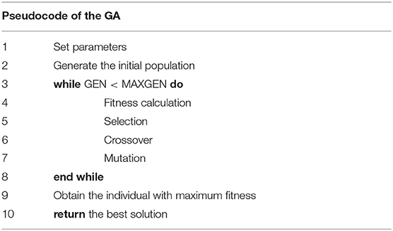
Algorithm 1. The pseudocode of a GA.

For the purposes of this study, a real-valued representation is adopted as encoding strategy. The use of real-valued genes in GAs offers over binary encodings the following advantages: (i) efficiency of the GA is increased as there is no need to convert chromosomes to phenotypes before each function evaluation, (ii) less memory is required as efficient floating point internal computer representations can be used directly, (iii) no loss in precision by discretization to binary or other values, (iv) greater freedom to use a variety of genetic operators.

Initialization of Population

The GA starts with the generation of a random initial population of individuals with uniform distribution in the initial generation. If the initial population is denoted by P₀ and its size (number of individuals) by n_P, then any element of P₀ is given by:

$\begin{array}{ll}{x}_{i,j}=x_{j,min}+(x_{j,max}-x_{j,min})a_{RU}& (14)\end{array}$

where a_RU is a random variable with uniform distribution for which 0 ≤ a_RU ≤ 1. It is ensured that x_i, i = {m+1, m+2, …, 2m} is a positive integer. In case of a duplicate integer found this is replaced by a random integer value (respecting the upper and lower bounds) different from the calculated ones in P₀.

Selection and Crossover

The stochastic universal sampling (SUS) is used as a selection function, which provides zero bias and minimum spread. SUS offers an offspring selection procedure that may lead to faster convergence to the solution of a problem than other selection methods, such as e.g., roulette wheel selection.

In addition, to avoid duplicate entries in the ground motion record identities a new crossover scheme is proposed which ensures that the linear combination of the ground motion records examined each time is comprised by unique members. This procedure is described by detail in the following:

If the crossover is performed between two random individuals at generation k, P_{k, 1} = {x_{i1, j}} and P_{k, 2} = {x_{i2, j}}, the individual P_{k+1, 12} is produced as a result of the crossover. Initially, three set operations are performed between the two individuals:

a) Intersection between x_{i1, j} and x_{i2, j}:

$\begin{array}{ll}{x}_{1\cap 2}=\left\{x_{i1,j}\right\}\bigcap \left\{x_{i2,j}\right\}& (15)\end{array}$

b) Subtraction of x_{i2, j} from x_{i1, j}:

$\begin{array}{ll}{x}_{1-2}=\left\{x_{i1,j}\right\}-\left\{x_{i2,j}\right\}& (16)\end{array}$

c) Subtraction of x_{i1, j} from x_{i2, j}:

$\begin{array}{ll}{x}_{2-1}=\left\{x_{i2,j}\right\}-\left\{x_{i1,j}\right\}& (17)\end{array}$

The offspring P_{k+1, 12} will contain the intersection x_1∩2 which contains n_1⋂2 elements and the vector {_{x1−2, x2−1}l} which contains l = m−n_1⋂2 randomly selected elements from the vector formed by concatenating the two differences {x₁₋₂, x₂₋₁}:

$\begin{array}{ll}{P}_{k+1,12}=\left\{x_{1\bigcap 2},{\left\{x_{1-2},x_{2-1}\right\}}_l\right\}& (18)\end{array}$

In the case where x_1∩2 = ∅ then {_{x1−2, x2−1}l} = {x₁₋₂, x₂₋₁}. Equations (15–18) apply both for continuous and integer design variables of the problem.

Mutation

In GA, the mutation function uses various distributions from which random numbers (perturbations) are generated and added to the components of the individual that is mutated. In this study, the perturbation of the continuous/integer design variables, is performed using a Gaussian/random uniform distribution, respectively, and are described in detail below.

Continuous variables

The mutation function of continuous design variables follows a Gaussian distribution of zero-mean with standard deviation given by the relation:

$\begin{array}{ll}{m}_{SC,k}=m_{SC,0}\left(1-m_{SH}\frac{k}{k_{max}}\right)& (19)\end{array}$

where the standard deviation m_{SC, k} is the fraction of the maximum range of possible perturbations of the design variables (i.e., scale factors) that can be added to an individual in generation k during mutation process. m_{SC, 0} is the scale parameter and is equal to the fraction of the maximum range of possible perturbations of the continuous variables at the initial generation (0), whereas m_SH is the shrink parameter which controls how fast m_{SC, k} is reduced as generations evolved. Both of the parameters m_{SC, 0} and m_SH can be arbitrarily selected and their values must be between 0 and 1. m_SH < 0 or m_SH > 1 is also possible, but not recommended. For a random individual at generation k, P_{k, 1} = {x_{i1, j}} this operation can be written as follows:

$\begin{array}{ll}{P}_{k+1,1}=\left\{x_{i1,j}\right\}+{ā}_{GU}{m}_{SC,k},1\le j\le m& (20)\end{array}$

where m_{SC, k} is given by Equation (19) and ā_GU is a vector with entries following a uniform Gaussian distribution.

Integer variables

The mutation function of integer design variables follows a random uniform distribution. Since the random perturbations are not integers in general, the result is rounded toward the nearest integer and then the remainder of its Euclidean division with M is extracted, to ensure that the result does not exceed M value. For a random individual at generation k, P_{k, 1} = {x_{i1, j}} this operation can be written as follows:

$\begin{array}{l}{P}_{k+1,1}=mod\left(\langle \left\{x_{i1,j}\right\}+(2{ā}_{RU}-1)m_{SC,k}\rangle ,M\right),\\ m+1\le j\le 2m& (21)\end{array}$

where the symbol 〈〉 is used to denote the nearest integer of the quantity contained in the brackets, ā_RU is a vector with entries following a uniform random distribution with 0 ≤ ā_{RU, j} ≤ 1, m_{SC, k} is the scale parameter of mutation function (standard deviation of Gaussian distribution at the k^th generation), and mod () denotes the modulo operation, i.e., the remainder of the Euclidean division of between the two arguments. After application of Equation (21) the result is checked for duplicate values of integer components. If so, the duplicates are replaced by a random integer value (respecting the upper and lower bounds) different from the calculated ones.

Numerical Results

The effectiveness of the proposed algorithm is verified by generation of artificial accelerograms which are compliant to target spectra of different inherent nature, ensuring also the independence of the algorithm's performance from the target spectrum. More specific, the acceleration and equivalent input energy velocity response spectra of three ground motion records: (a) El Centro Terminal Substation Building record of the 1940 Imperial Valley earthquake, (b) Rinaldi record of the 1994 Northridge earthquake and (c) Sakarya—SKR record of the 1999 Kocaeli earthquake are defined as target spectra. The target spectra are associated with a far-field ground motion, a near-field ground motion which contains forward directivity effects and a near-field ground motion which contains fling-step effects, respectively (Kalkan and Kunnath, 2006). Typical characteristic of the near-field motions is the presence of high-velocity pulses, which do not exist in typical far-field ground motions. The difference between these two types of motions originates mainly from two factors: (a) the distance between the site where the earthquake is recorded and the seismic fault, (b) the orientation of the last. It is noted that the three target spectra have essentially different general configurations, a fact that results from the different inherent nature of the time histories of the three ground motions.

Two matching scenarios are considered: (i) Matching Scenario 1 (Sa matching): Matching only the spectral acceleration and (ii) Matching Scenario 2 (Sa–Vei matching): Matching both the spectral acceleration and the equivalent input energy velocity spectra (absolute and relative). In each scenario, the database is comprised of the ground motion records obtained from the European Strong Motion (ESD) database (Ambraseys et al., 2004; Iervolino et al., 2010). After a preliminary screening of the ESD database, a subset database is constructed that consists of 6026 ground motion records corresponding to horizontal earthquake components, i.e., M = 6026. The number m of ground motion records in the suite is set to be equal to 20 and the matching range of periods is between T₁ = 0.1 s and T₂ = 4.0 s. The penalty constant k_p is set to be equal to 50.

Furthermore, the tuning parameters of the GA are selected as follows: the population size n_p (number of individuals in each generation) is equal to 80. For reproduction, the number of individuals that are guaranteed to survive to the next generation (elite children) is equal to 5% of the population size, namely n_E = 0.05n_P = 4, and the fraction of the next generation, other than elite children, that is produced by crossover (crossover fraction) is equal to 0.8, i.e., n_C = 0.8(n_P−n_E)≈61 individuals are produced in each generation. The number of individuals in each generation that are produced by mutation is n_M = n_P−n_E−n_C = 15. In the GA used in this study no migration occurs, as there are no subpopulations. As stopping criteria for the GA algorithm the maximum number of generations (MAXGEN) is used, i.e., equal to 100. A sensitivity analysis of 30 independent optimization runs is also performed followed by a statistical process on the optimized results. The sensitivity analysis represents a necessary step since the GA optimization procedure does not yield the same results when restarted due to its stochastic nature.

In all cases examined, the objective function is evaluated using OpenSeismoMatlab, an open source tool for earthquake ground motion processing (Papazafeiropoulos and Plevris, 2018). OpenSeismoMatlab performs baseline correction and generates the elastic acceleration and equivalent input energy velocity response spectra which are then used for the calculation of the objective function.

Matching Scenario 1

The optimization results for Matching Scenario 1 are depicted in Figure 1. For each target record, the black curve represents the target acceleration spectrum, while the red and blue curves represent the spectral acceleration that corresponds to the optimization run (out of the 30 runs) that fits best and worst to the target spectrum, respectively. The coefficient of variation (CoV) of the 30 runs for each period is also depicted by the green curve.

FIGURE 1

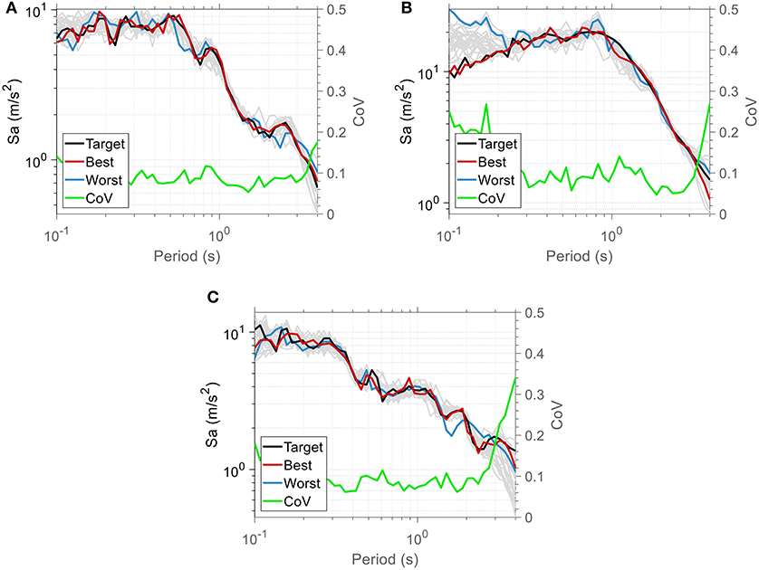
Figure 1. Optimization results of Matching Scenario 1 for each target: (A) El Centro, (B) Northridge, and (C) Sakarya.

A good agreement is observed between the “best” and “target” spectra in all cases examined while the CoV value increases near the bounds of the matching period range. This is mostly attributed to the range of the periods involved in the calculation of the objective value [see Equations (9) and (10)] which is defined in a way that it covers the eigenperiods of a structure. This means that the period range used in the matching procedure and consequently the optimized acceleration time history are period-dependent. In this study, an extended period range is selected to highlight the applicability of the proposed methodology for a variety of structures. However, most of civil structures have eigenperiods that are concentrated near the middle of the range considered, where the CoV values are minimum and high accuracy can be achieved. Furthermore, the finite number of ground motions in the suite of the linear combination contributes to large CoV values in general. As the number of the ground motions in the suite decreases, the methodology becomes more cumbersome, since the time history given by the suite has less flexibility. Hence, as the number of the ground motions increases, the matching becomes generally better. Finally, the shape of the penalty function in Equation (11) has an important effect on the optimized response spectrum of each optimization run, since the weighting of the deviation from the target spectrum for the matching period range considered is not uniform, as has been already mentioned in the previous section.

Figure 2 shows the convergence history of the 30 independent optimization runs of Matching Scenario 1. Each curve represents the objective value of the best individual at each generation of a given optimization run. The red (blue) curve represents the evolution of the objective value that corresponds to the optimization run (out of the 30 runs) that fits best (worst) to the target spectrum.

FIGURE 2

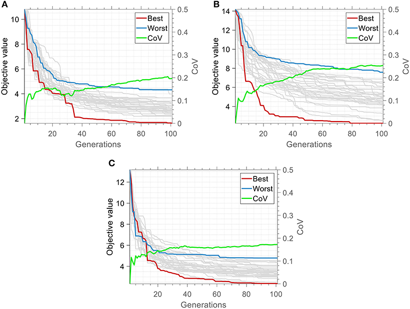
Figure 2. Optimization history of the 30 independent runs of the Matching Scenario 1 for each target: (A) El Centro, (B) Northridge, and (C) Sakarya.

It can be noted that in the case of El Centro earthquake the best individual of the final generation for the best independent run corresponds to roughly 14% of the objective value of the best individual of the initial generation. The best individual of the final generation for the worst independent run corresponds to roughly 40.3% of the objective value of the best individual of the initial generation. In the case of Northridge earthquake these percentages are roughly equal to 16.1% and 53.6%, and in the case of Sakarya earthquake they are 17.7% and 36.9% respectively.

The trend of all convergence histories shows that the approach to the optimum value is quick and relatively smooth, which is achieved by proper adjustment of the crossover and mutation rates, in order to ensure sufficient population diversity in each generation. It seems that, while the coefficient of variation among the optimization histories increases at the early stages of the optimization process, there is a point after which it stabilizes until termination. The magnitude of the final stabilized value of the CoV value is a measure of the complexity of the optimization space. As it is expected, larger CoV values corresponds to increased diversity between the various optimization runs, in terms of the path followed by the best individual of each optimization run. The largest CoV value of the objective value of the best individual among the various optimization runs at the final generation occurs in the case of Northridge earthquake, an observation that correlates well with the large dispersion of the optimum spectra, especially in the low period range, in Figure 1B.

Matching Scenario 2

The optimization results for Matching Scenario 2 are depicted in Figure 3. Nearly the same traits that are mentioned for Figure 1 are observed; the proposed algorithm gives higher CoV values in the lower and higher limits of the matching period range considered.

FIGURE 3

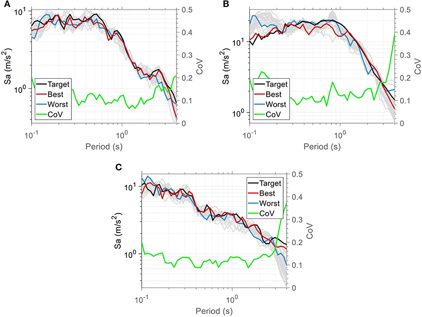
Figure 3. Results of Matching Scenario 2 regarding spectral acceleration for each target: (A) El Centro, (B) Northridge, and (C) Sakarya.

In Figures 4, 5, the absolute seismic input energy equivalent velocity (S_ievABS) and the relative seismic input energy equivalent velocity (S_ievREL) spectra for each target spectrum are presented, respectively. A very close agreement between the target and corresponding optimized spectra is also observed in this case. Although the CoV plots exhibit local peaks and troughs, all of them fluctuate around the value of 10%, regardless of the target spectrum.

FIGURE 4

Figure 4. Results of Matching Scenario 2 regarding equivalent absolute seismic input energy velocity spectra (SievABS) for each target: (A) El Centro, (B) Northridge, and (C) Sakarya.

FIGURE 5

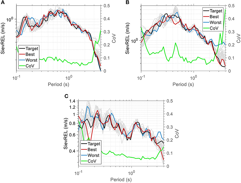
Figure 5. Results of Matching Scenario 2 regarding equivalent relative seismic input energy velocity spectra (SievREL) for each target: (A) El Centro, (B) Northridge, and (C) Sakarya.

In a similar rationale, Figure 6 depicts the convergence history of the 30 independent optimization runs of Matching Scenario 2. It is apparent that in the case of El Centro earthquake the best optimization run gives result equal to 32.8% of the best objective value of the initial population, whereas the worst result is roughly equal to 48.3% of the initial best objective value. In the case of Northridge earthquake the best and worst results are roughly equal to 32 and 55.7% respectively of the initial best objective value. Similarly, the corresponding percentages for the Sakarya earthquake are 26 and 41.1%. Interestingly, the lowest (best) percentage appears in the case of Sakarya earthquake whereas the highest (worst) percentage appears in the case of Northridge earthquake. The smooth convergence in optimization histories demonstrates the reliability of the proposed algorithm not only for matching the target spectral acceleration, but also for matching both target acceleration and target seismic input energy equivalent velocity spectra.

FIGURE 6

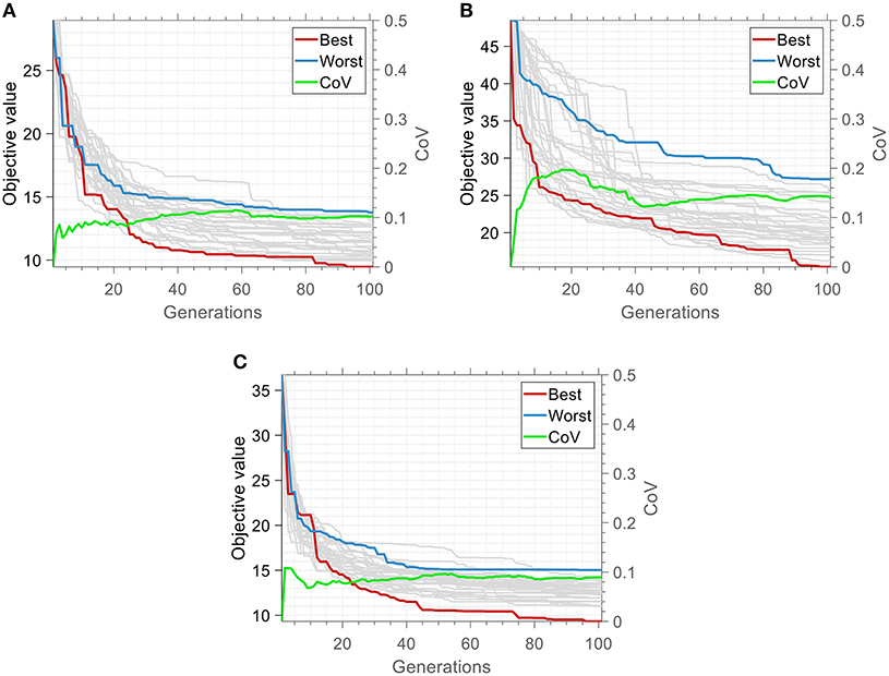
Figure 6. Optimization history of the 30 independent runs of the Matching Scenario 2 for each target: (A) El Centro, (B) Northridge, and (C) Sakarya.

Scenarios Comparison

A one-to-one comparison between the performance of the two scenarios shows that the CoV is generally higher in Scenario 2. This occurs because the optimization problem of Scenario 1 is more “relaxed” than the Scenario 2. In Scenario 1, the objective function is related only with a single target spectrum (acceleration), while in Scenario 2 the objective function is related with three target spectra (acceleration, absolute velocity, relative velocity), at the same time. This relation establishes an indirect “constraint” which implies that, with respect to the target acceleration spectrum only, the optimized solution of Scenario 2 will have higher deviation than that of Scenario 1, which interprets the higher CoV values in Figure 3 when compared to Figure 1. Consequently, in the case of Scenario 2 the possible “paths” of the population evolution toward the optimum are far fewer and therefore the population diversity is lower compared to Scenario 1, which explains the reduced CoV in the last generation in Figure 6 (Scenario 2), compared to that in Figure 2 (Scenario 1). Finally, it is noted that as the generations increase, the CoV fluctuation is smoother in the case of Scenario 2, related to the increased robustness of the algorithm in this case.

Verification of the Proposed Methodology

In order to assess the robustness and accuracy of the proposed methodology the seismic performance of single- and multi- degree of freedom structural systems has been considered. To this end, nonlinear response history analyses were conducted for the optimized accelerograms of the two Matching Scenarios as resulted for the three target ground motion records in Section 3. The response results are compared in terms of the goodness-of-fit with the respective response result of the target ground motion. The seismic input energy that is dissipated due to viscous damping action in the structure (damping energy) is also quantified.

Energy Definitions

The seismic input energy that is absorbed by an inelastic single degree of freedom (SDOF) structural system during an earthquake can be defined by integrating the equation of motion of the system as follows:

$\begin{array}{ll}{\displaystyle \underset{0}{\overset{u}{\int }}}ü\bar{m}du+{\displaystyle \underset{0}{\overset{u}{\int }}}\stackrel{.}{u}\bar{c}du+{\displaystyle \underset{0}{\overset{u}{\int }}}{f}_{s}du=-{\displaystyle \underset{0}{\overset{u}{\int }}}\bar{m}\left\{I\right\}{ü}_{g,c}du& (22)\end{array}$

where $\bar{m}$ is the mass matrix, $\bar{c}$ is the viscous damping coefficient matrix, f_s is the resistance force due to stiffness, I is the unit influence vector of the structure and ü_{g, c} is the linear combination of the accelerations of ground motions records in the suite as defined in section resampling Equation (22) stands as a statement of energy balance of the system and can be rewritten as:

$\begin{array}{ll}{E}_k(t)+E_d(t)+E_s(t)+E_y(t)=E_I(t)& (23)\end{array}$

With regard to Equation (22) the first integral gives the kinetic energy E_k, the integral on the right-hand side gives the input energy E_I imparted from the ground motion to the structure and the last integral on the left-hand side is equal to the sum of the linear elastic recoverable strain energy E_s and the plastic irrecoverable strain energy E_y. The damping energy term E_d is defined as follows:

$\begin{array}{ll}{E}_d(t)={\displaystyle \underset{0}{\overset{u}{\int }}}\stackrel{.}{u}\bar{c}du.& (24)\end{array}$

The definitions of the aforementioned energy quantities are given for a structure whose mass is acted upon by a force equal to $p_{eff}(t)=-\bar{m}\left\{I\right\}{ü}_{g,c}$, i.e., they are based on the consideration of the structural motion relative to the base, rather than the total motion of the structure. The two types of energy formulations (relative and absolute) are equivalent but the former is more intuitive and simplifies the calculations when it comes to multi degree of freedom (MDOF) structural systems. Equations (22–24) correspond to a SDOF system in mathematical terms and their extension to MDOF systems can be done in a straightforward manner.

SDOF System Results

Three SDOF systems involving a bilinear elastoplastic constitutive model with kinematic hardening are analyzed for each target ground motion. The eigenperiod, the critical damping ratio, the post-yield stiffness ratio (i.e., the ratio of the post-yield stiffness to the initial small strain stiffness of the structure), and the ductility demand are same for all the SDOF systems and equal to 0.5 sec, 5%, 1%, and 1.1, respectively. The three systems have different yield displacements, equal to 0.052, 0.1, and 0.025 m for the El Centro, the Northridge and the Sakarya target ground motion, respectively. The reader is referred to Papazafeiropoulos et al. (2017) for more details about the implementation of the bilinear elastoplastic constitutive model with kinematic hardening and the time integration algorithm that were used in this study.

The small ductility value specified for all target ground motions denotes that structures only with slightly nonlinear behavior are considered in this study; for cases of severely nonlinear response the scenarios presented in this study for calculation of the design artificial ground motion is an open research issue. For such cases it would be better to consider the inelastic response spectra, rather than elastic response spectra in matching scenarios. In addition, the physical properties of each SDOF system remain the same for the estimation of its dynamic response for each target ground motion as well as the optimized ground motions obtained from the two matching scenarios. Based on an arbitrarily selected value of ductility demand (equal to 1.1, to ensure a slightly nonlinear response) for each target ground motion the yield displacement that is calculated was used also for the corresponding optimized ground motions obtained from the two matching scenarios in all nonlinear time history response analyses.

In Figure 7, the time variation of the damping energy per unit mass for each target motion and the optimized ground motion records produced from the two matching scenarios is depicted. A good agreement is observed in all cases since the damping energy of the optimized ground motion (red line) is very close to that of the respective target ground motion (black line). To quantify this agreement, the normalized error e_ij for the i^th story (in the case of SDOF systems i is always equal to 1) and j^th matching scenario, which is proportional to the area between a matching scenario and the target ground motion curves was used as a metric of this goodness-of-fit, defined as follows:

$\begin{array}{ll}{e}_{ij}=\frac{{\displaystyle \underset{0}{\overset{T_d}{\int }}\left|E_{d,i}^j\left(t\right)-E_{d,i}^T\left(t\right)\right|dt}}{{\displaystyle \underset{0}{\overset{T_d}{\int }}{E}_{d,i}^T\left(t\right)dt}}.& (25)\end{array}$

where $E_{d,i}^j$ and $E_{d,i}^T$ is the damping energy for the j^th scenario and the target ground motion, respectively.

FIGURE 7

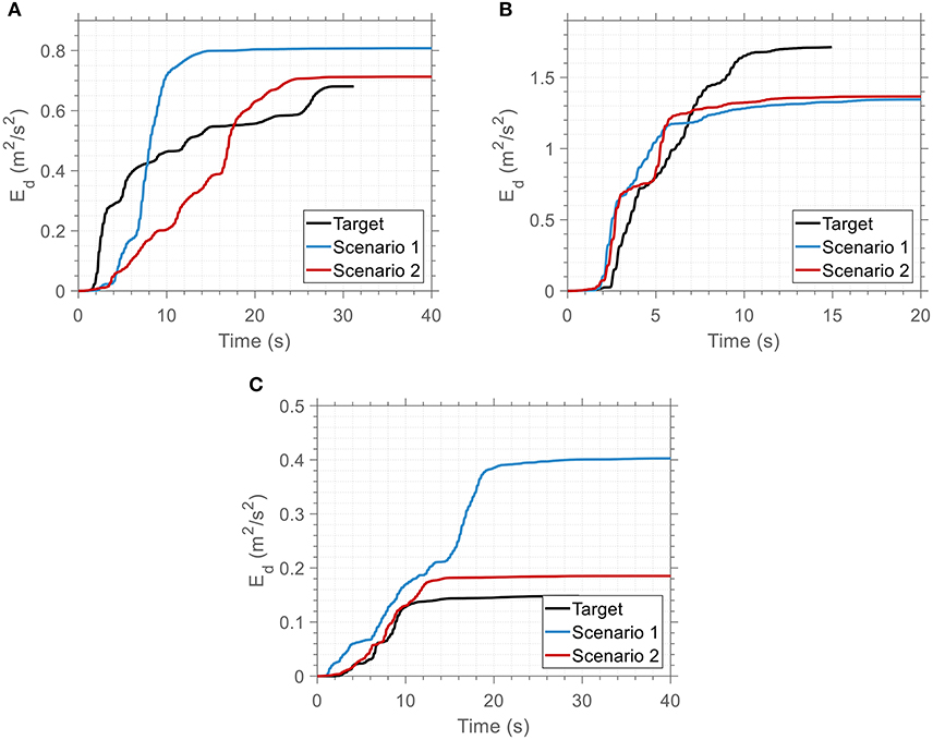
Figure 7. Energy dissipated by viscous damping per unit mass over time for the optimized artificial ground motions of the two matching scenarios and for each target ground motion: (A) El Centro, (B) Northridge, and (C) Sakarya.

Even in the case of Northridge target ground motion, it is indicative that the damping energy corresponding to Scenario 2 is slightly closer to the respective curve of the target motion, although there is not much difference between the two scenarios (17% as seen in Table 1). This fact, in combination with the large value of the dissipated energy per unit mass may be a consequence of the special characteristics of Northridge earthquake, which contains a high velocity pulse (forward directivity effect) as a near-field ground motion.

TABLE 1

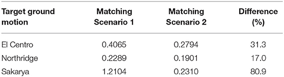
Table 1. Normalized error of the damping energy between the optimized and the target ground motion records.

MDOF System Results

Two model buildings were analyzed as a 3-DOF and 9-DOF structural systems. More specific, the model buildings are a 3-story (LA3) and a 9-story building (LA9) designed as standard office buildings and situated on a stiff soil (soil type S2), following the local code requirements for the Los Angeles city (UBC, 1994), and according to the provisions of the FEMA/SAC project, presented in FEMA 355C (2000). The plan and elevation of their effective structural models, along with the various cross sections of its members are shown in Supplementary Figure 1. The perimeter moment-resisting frames act as the structural system of the building. The column bases of the moment resisting frames are considered as fixed. Furthermore, the design of the buildings for the two orthogonal directions is quite similar, and therefore only half of the structure is considered in the analysis in each case.

The benchmark buildings are simulated as a 3-DOF and a 9-DOF structural system involving the same bilinear elastoplastic constitutive model with kinematic hardening, as in the SDOF system analyzed previously. Their fundamental eigenperiods are equal to 1.01 and 2.85 sec, respectively. The post-yield stiffness ratio and critical damping ratio were set equal to 1% and 5%, respectively. The yield displacement and ductility demand of each story for the 3-DOF and 9-DOF structural systems are shown in Table 2. The maximum ductility at any story does not exceed the value of 2. Usually, an interpolative iterative procedure is necessary to obtain the yield displacement for a target ductility demand (Chopra, 2017). However, for each target ground motion in each building the yield displacement is assumed as uniform distributed across all stories and is calculated so that the maximum ductility demand is equal to 2 at least in one story of the building. For both of the LA3 and LA9 buildings the maximum ductility demand is observed at the first story. The ductility of the remaining stories is much lower or even lower than 1 (i.e., story remains linear elastic).

TABLE 2

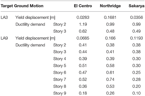
Table 2. Yield displacement and ductility demand of each story for the 3-DOF and 9-DOF structural systems.

For each target ground motion, three nonlinear response history analyses were conducted using as excitation the target ground motion and the two optimized ground motions resulting from the two matching scenarios. Figures 8–10 show the time history of the damping energy at the three stories of the building for each target ground motion and the optimized ground motion records. Again, a good agreement is observed in all cases since the damping energy of the optimized ground motion (red line) is very close to that of the respective target ground motion (black line).

FIGURE 8

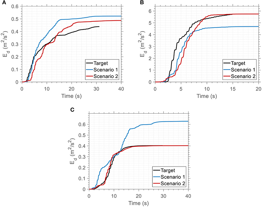
Figure 8. Time variation of energy dissipated at the 1st story of the 3-DOF system for the optimized and the target ground motion records: (A) El Centro, (B) Northridge, and (C) Sakarya.

FIGURE 9

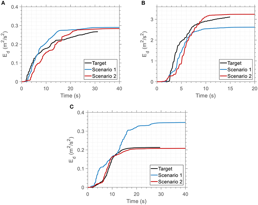
Figure 9. Time variation of energy dissipated at the 2nd story of the 3-DOF system for the optimized and the target ground motion records: (A) El Centro, (B) Northridge, and (C) Sakarya.

FIGURE 10

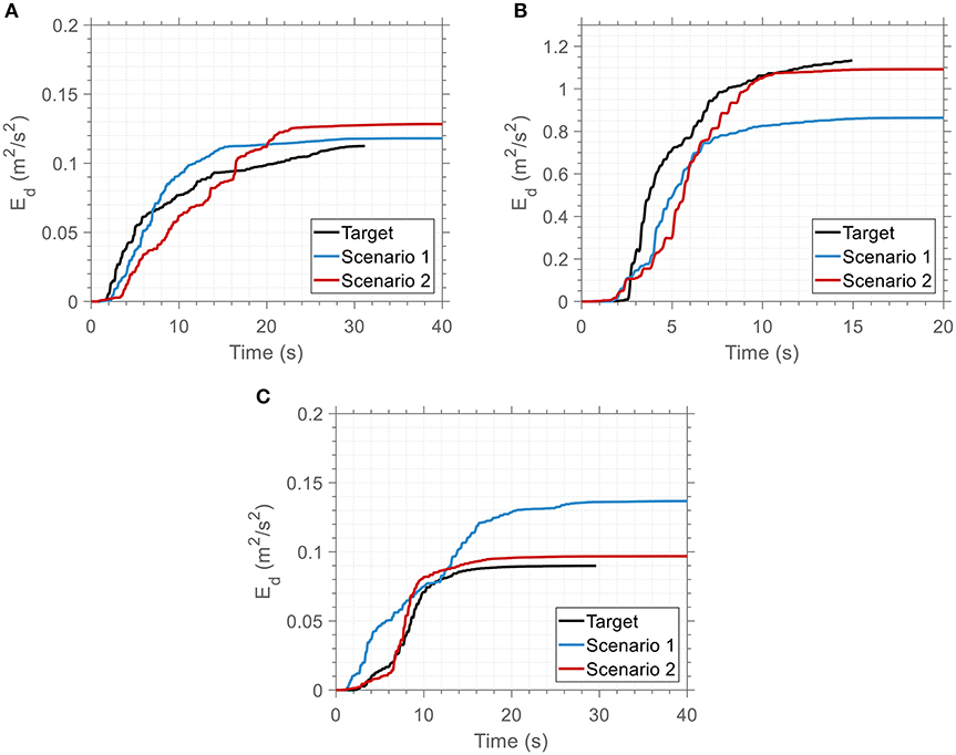
Figure 10. Time variation of energy dissipated at the 3^rd story of the 3-DOF system for the optimized and the target ground motion records: (A) El Centro, (B) Northridge, and (C) Sakarya.

FIGURE 11

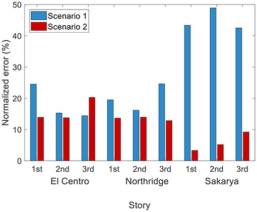
Figure 11. Normalized error of the damping energy between the optimized and the target ground motion records for each floor of the 3-DOF structural system.

To quantify this agreement the normalized error as defined in Equation (25) was used as a metric of this goodness-of-fit. Figure 11 shows the normalized error of the damping energy between the optimized and the target ground motion records for each floor of the 3-DOF structural system. The min/max errors for the two scenarios are 15%/48% and 3%/20%, respectively. It is observed that the proposed algorithm (Scenario 2) yields far lower error compared to Scenario 1. Although the error of Scenario 2 remains lower, only in the case of the dynamic response of the third floor of the 3-DOF system for the El Centro target motion Scenario 2 gives greater error compared to Scenario 1 (28% higher). It is worth noting that in the case of the Sakarya target ground motion the error of the Scenario 2 is 78.3% lower compared to Scenario 1. This is directly related with the low CoV values observed in Section 3 for this specific case, a fact that also proves the robustness and accuracy of the proposed methodology.

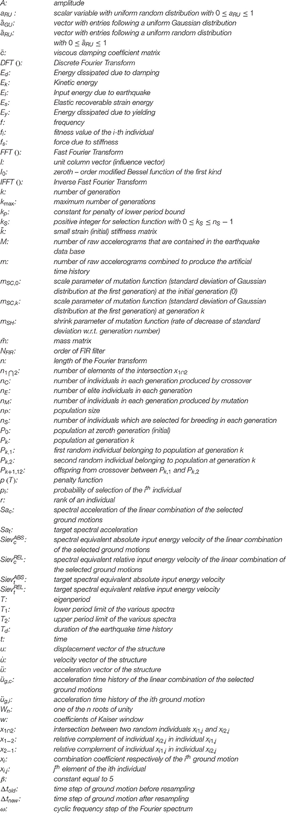
Figure 12 shows the time history of the damping energy at a typical story (i.e., first story) of the LA9 building for each target ground motion and the optimized ground motion records. Again, a good agreement is observed in all cases since the damping energy of the optimized ground motion is very close to that of the respective target ground motion. To quantify this agreement, Figure 13 shows the normalized error of the damping energy between the optimized and the target ground motion records for each story of the 9-DOF structural system. The min/max errors for the two scenarios are 8.2%/88.7% and 9.8%/38.5%, respectively. It is observed that the proposed algorithm (Scenario 2) yields far lower error compared to Scenario 1. The error of Scenario 2 remains higher, only in the case of the dynamic response of the upper stories of the 9-DOF system for the Northridge target motion. This deviation is attributed to the dynamic characteristics of the structural system mainly affected by the near field effects of the specific ground motion. It is worth noting that the maximum error of the Scenario 1 is 130.4% higher compared to the corresponding maximum error of the Scenario 2.

FIGURE 12

Figure 12. Time variation of energy dissipated at the 1st story of the 9-DOF system for the optimized and the target ground motion records: (A) El Centro, (B) Northridge, and (C) Sakarya.

FIGURE 13

Figure 13. Normalized error of the damping energy between the optimized and the (A) El Centro, (B) Northridge, and (C) Sakarya target ground motion records for each floor of the 9-DOF structural system.

Conclusions

In this study a novel spectra-matching framework is developed, which employs a linear combination of raw ground motion records to generate artificial accelerograms. To this end, apart from the well-known design acceleration spectrum that is prescribed by the various norms and guidelines, the seismic input energy equivalent velocity spectrum is also taken into account.

This consideration is leading therefore to optimized acceleration time histories, which represent actual motions in a much more realistic way. In order to produce elastic spectra that match as closely as possible to a given target spectrum, the procedure of selection and scaling of a suite of ground motion records to fit a given target spectrum is formulated as an optimization problem. Three characteristic ground motion records of different inherent nature are selected as target spectra, to verify the effectiveness of the proposed algorithm, ensuring that its performance is not ground motion record-dependent assuming different matching scenarios. The optimization results have shown that there exists a good agreement between the target and optimized spectra for each case examined, regardless of the nature of target spectrum. Finally, it is proved that the artificially generated records are much more realistic and suitable for the seismic design of structures, since they reproduce better the real non-linear structural inelastic response in terms of the damping energy, demonstrating also the reliability and robustness of the proposed methodology.

Data Availability Statement

The datasets generated for this study are available on request to the corresponding author.

Author Contributions

GP had the research idea, drafted the article, did the data collection, contributed in the numerical analysis of the numerical examples, and wrote the paper. MG analyzed and interpreted the data, contributed in the conception and design of the work, wrote the paper, and supervised the overall research work. MP supervised the overall research work.

Conflict of Interest

The authors declare that the research was conducted in the absence of any commercial or financial relationships that could be construed as a potential conflict of interest.

Supplementary Material

The Supplementary Material for this article can be found online at: https://www.frontiersin.org/articles/10.3389/fbuil.2019.00140/full#supplementary-material

References

Akiyama, H. (1985). Earthquake-Resistant Limit-State Design for Buildings. Tokyo: University of Tokyo Press.

Google Scholar

Ambraseys, N., Smit, P., Douglas, J., Margaris, B., Sigbjörnsson, R., and Olafsson, S. (2004). Internet site for European strong-motion data. Bollettino di geofisica teorica ed applicata, 45, 113–129. Available online at: http://www3.ogs.trieste.it/bgta/provapage.php?id_articolo=225

Google Scholar

Atkinson, G. M., and Goda, K. (2010). Inelastic seismic demand of real versus simulated ground-motion records for cascadia subduction earthquakesinelastic seismic demand of real versus simulated ground-motion records for subduction earthquakes. Bull. Seismol. Soc. Am. 100, 102–115. doi: 10.1785/0120090023

CrossRef Full Text | Google Scholar

Boore, D. M. (2009). Comparing stochastic point–source and finite–source ground–motion simulations: SMSIM and EXSIM. Bull. Seismol. Soc. Am. 99, 3202–3216. doi: 10.1785/0120090056

CrossRef Full Text | Google Scholar

Chapman, M. C. (1999). On the use of elastic input energy for seismic hazard analysis. Earthq. Spect. 15, 607–635. doi: 10.1193/1.1586064

CrossRef Full Text | Google Scholar

Chopra, A. K. (2017). Dynamics of Structures, 5th Edn. Pearson: University of California at Berkeley.

Google Scholar

Chou, C.-C., and Uang, C.-M. (2003). A procedure for evaluating seismic energy demand of framed structures. Earthq. Eng. Struct. Dyn. 32, 229–244. doi: 10.1002/eqe.221

CrossRef Full Text | Google Scholar

Dindar, A. A., Yalçin, C., Yüksel, E., Özkaynak, H., and Büyüköztürk, O. (2015). Development of earthquake energy demand spectra. Earthq. Spect. 31, 1667–1689. doi: 10.1193/011212EQS010M

CrossRef Full Text | Google Scholar

FEMA 355C (2000). Federal Emergency Management Agency. State of the Art Report on Systems Performance of Steel Moment Frames Subject to Earthquake Ground Shaking. FFTW. Retrieved from: http://www.fftw.org (accessed November, 2019).

Google Scholar

Frigo, M., and Johnson, S. G. (1998). “FFTW: an adaptive software architecture for the FFT,” in Paper Presented at the Proceedings of the 1998 IEEE International Conference on Acoustics, Speech and Signal Processing, ICASSP'98 (Cat. No. 98CH36181) (Seattle, WA). doi: 10.1109/ICASSP.1998.681704

CrossRef Full Text | Google Scholar

Graves, R. W., and Pitarka, A. (2010). Broadband ground-motion simulation using a hybrid approach. Bull. Seismol. Soc. Am. 100, 2095–2123. doi: 10.1785/0120100057

CrossRef Full Text | Google Scholar

Holland, J. H. (1992). Adaptation in Natural and Artificial Systems: An Introductory Analysis With Applications to Biology, Control, and Artificial Intelligence. Cambridge, MA: MIT Press. doi: 10.7551/mitpress/1090.001.0001

CrossRef Full Text | Google Scholar

Iervolino, I. C, Galasso, E., and Cosenza (2010). REXEL: computer aided record selection for code-based seismic structural analysis. Bull. Earthq. Eng. 8, 339–362. doi: 10.1007/s10518-009-9146-1

CrossRef Full Text | Google Scholar

Iervolino, I., Maddaloni, G., and Cosenza, E. (2008). Eurocode 8 compliant real record sets for seismic analysis of structures. J. Earthq. Eng. 12, 54–90. doi: 10.1080/13632460701457173

CrossRef Full Text | Google Scholar

Jiao, Y., Yamada, S., Kishiki, S., and Shimada, Y. (2011). Evaluation of plastic energy dissipation capacity of steel beams suffering ductile fracture under various loading histories. Earthq. Eng. Struct. Dyn. 40, 1553–1570. doi: 10.1002/eqe.1103

CrossRef Full Text | Google Scholar

Kalkan, E., and Kunnath, S. K. (2006). Effects of fling step and forward directivity on seismic response of buildings. Earthq. Spect. 22, 367–390. doi: 10.1193/1.2192560

CrossRef Full Text | Google Scholar

Katsanos, E., Sextos, A. G., and Manolis, G. D. (2010). Selection of earthquake ground motion records: a state-of-the-art review from a structural engineering perspective. Soil Dyn. Earthq. Eng. 30, 157–169. doi: 10.1016/j.soildyn.2009.10.005

CrossRef Full Text | Google Scholar

Kuwamura, H., and Galambos, T. V. (1989). Earthquake load for structural reliability. J. Struct. Eng. 115, 1446–1462. doi: 10.1061/(ASCE)0733-9445(1989)115:6(1446)

CrossRef Full Text | Google Scholar

Leelataviwat, S., Saewon, W., and Goel, S. C. (2009). Application of energy balance concept in seismic evaluation of structures. J. Struct. Eng. 135, 113–121. doi: 10.1061/(ASCE)0733-9445(2009)135:2(113)

CrossRef Full Text | Google Scholar

López Almansa, F., Yazgan, A. U., and Benavent Climent, A. (2013). Design energy input spectra for high seismicity regions based on Turkish registers. Bull. Earthq. Eng. 11, 885–912. doi: 10.1007/s10518-012-9415-2

CrossRef Full Text | Google Scholar

Papazafeiropoulos, G., and Plevris, V. (2018). OpenSeismoMatlab: a new open-source software for strong ground motion data processing. Heliyon 4:e00784. doi: 10.1016/j.heliyon.2018.e00784

CrossRef Full Text | Google Scholar

Papazafeiropoulos, G., Plevris, V., and Papadrakakis, M. (2017). A new energy-based structural design optimization concept under seismic actions. Front. Built Environ. 3:44. doi: 10.3389/fbuil.2017.00044

CrossRef Full Text | Google Scholar

Surahman, A. (2007). Earthquake-resistant structural design through energy demand and capacity. Earthq. Eng. Struct. Dyn. 36, 2099–2117. doi: 10.1002/eqe.718

CrossRef Full Text | Google Scholar

Tselentis, G., Danciu, L., and Sokos, E. (2010). Probabilistic seismic hazard assessment in Greece–Part 2: acceleration response spectra and elastic input energy spectra. Nat. Hazards Earth Syst. Sci. 10, 41–49. doi: 10.5194/nhess-10-41-2010

CrossRef Full Text | Google Scholar

Uang, C.-M., and Bertero, V. V. (1988). Use of Energy as a Design Criterion in Earthquake-Resistant Design, Vol. 88. Richmond, CA: Earthquake Engineering Research Center, University of California at Berkeley.

Google Scholar

Uang, C.-M., and Bertero, V. V. (1990). Evaluation of seismic energy in structures. Earthq. Eng. Struct. Dyn. 19, 77–90. doi: 10.1002/eqe.4290190108

CrossRef Full Text | Google Scholar

Uniform Building Code (UBC) (1994). International Conference of Building Officials. Whittier, CA.

Google Scholar

Zahrah, T. F., and Hall, W. J. (1984). Earthquake energy absorption in SDOF structures. J. Struct. Eng. 110, 1757–1772. doi: 10.1061/(ASCE)0733-9445(1984)110:8(1757)

CrossRef Full Text | Google Scholar

Nomenclature