Sensor Data Interpretation in Bridge Monitoring—A Case Study

Introduction

Structures such as bridges are increasingly being monitored for ensuring safety and for taking appropriate retrofit actions on time. National codes have begun to mandate sensor installation on large structures (Moreu et al., 2018). Traditionally, measurements are taken during load tests to compare as-built performance with that expected from the design. Recently, structural responses have been used for other purposes as well, such as, construction monitoring and occupancy tracking (Pan et al., 2017; Poston et al., 2017; Harichandran et al., 2019). Conventionally, strain gauges and accelerometers are fixed on structures with wired connections to data acquisition systems. Now, camera based non-contact vision sensors have emerged as a promising alternative to conventional contact sensors for health monitoring (Brownjohn et al., 2017; Feng and Feng, 2018; Ngeljaratan and Moustafa, 2019). While sensor technology has progressed rapidly, methodologies for extracting useful information from data and incorporating them into the decision making process have not matured. Most work on data interpretation focus on removing unwanted effects from data in order to isolate useful information. For example, Kromanis and Kripakaran (2017) discuss about separating the effects of temperature from structural response. Zhu et al. (2019) use Moving Principal Component Analysis (MPCA) for accounting for temperature variations to detect structural anomalies. Very few researchers have focused on issues related to visualization, decision making and user interfaces. A few examples include Napolitano et al. (2019), Glisic et al. (2014), and Zonta et al. (2014).

In many cases, measurements are just used to generate alarms when measured values exceed the bounds computed using theoretical calculations. This is useful for detecting serious faults and damage. More sophisticated methods involve detecting changes in the dynamic or static response of structures (Posenato et al., 2010). For example, wavelet analysis has been reported to offer superior performance especially for low levels of damage (Chouinard et al., 2019). A review of damage identification methods for bridges is given in An et al. (2019).

However, in many cases, structures that are monitored are not necessarily damaged and might have gradual deterioration. Here, the challenge is in determining the condition of the structure from their responses. Traditionally, this is known as the system identification task. System Identification is an inverse problem in which the properties of the system are inferred from the observations of its output.

System identification is widely used in various fields of engineering including structural engineering. A review of structural system identification methods is given in Sirca and Adeli (2012). Major structural system identification approaches are classified as follows:

• Model Calibration

• Probability based (e.g., Bayesian approach)

• Population based (e.g., model falsification)

• Model-free (e.g., using statistical learning)

Model calibration approach has been widely used for data interpretation for many years. This approach is also known as model updating or residual minimization. In this approach, the right structural model is obtained by minimizing the difference between measured values and predicted values. One of the major assumptions in this approach is that the parameter values chosen governs the difference between measured values and predicted values (Mottershead et al., 2011).

Even though model calibration is adopted by many researchers around the world, there are some fundamental shortcomings associated with this method. Unique solutions may not exist for inverse problems (Robert-Nicoud et al., 2005a; Beven, 2009; Raphael and Smith, 2013). Beyond the model structure within which they are calibrated, the parameter values may not be physically interpretable (Beven, 2000). So, parameters calibrated by this approach cannot be used to extrapolate outside the structure of the model as well as for other models. Residual minimization method cannot be used in situations involving presence of systematic bias or simplification of models (Robert-Nicoud et al., 2005b; Goulet et al., 2013a). Ben-Haim and Hemez showed that if the model is highly dependent on the test data, it will result in reduction in robustness and limited understanding of process (Ben-Haim and Hemez, 2012).

In the Bayesian approach, the prior knowledge of the parameters is updated using the observations from structural monitoring by use of Bayesian conditional probability (Beck, 2010). The likelihood function and observed data are used to update the probability distribution of parameters (Beck and Katafygiotis, 1998). The Bayesian approach can also be used for selecting model classes based on the measured data by comparing their relative credibility (Berger and Pericchi, 1996; Jeffreys, 1998). Only relative suitability of the model classes is obtained through this approach. Selection of wrong model classes in the primary stage cannot be identified by this approach (Goulet, 2012).

Bayesian approach can accommodate errors in observation or modeling, and can be applied in cases where the experimental data is incomplete (Goller et al., 2012). This approach is extensively used for various applications including structural identification. In complex scenarios which involve large uncertainties, development of probability distributions at measurement locations is extremely challenging (Soman et al., 2017). Parameters will be subjected to over conditioning when we try to simplify the probability distribution (Beven, 2000). To avoid bias in this approach, it is necessary to have complete knowledge about entire error correlation between locations of measurement (Goulet et al., 2013a,b).

In the population based approach, the goal is to identify a set of candidate models that reasonably explain observations. A model is selected to be a candidate if its predictions match the measurements at each and every sensor location within the threshold of modeling and measurement errors. Measurement errors are estimated using the sensor precision data. Estimating modeling errors is more complex and involves specific knowledge about the domain (Vernay et al., 2015). The falsification process starts with generating a discrete population of model instances which are created by randomly (or systematically) assigning values to parameters of a model class that have uncertainties. Since a large number of combinations of parameter values are possible and it is computationally expensive to evaluate each and every combination, a representative population is selected as the initially model set. The prediction of each model in the population is compared with the measurement at each sensor location and if the difference is greater than the error threshold, the model is eliminated from the set. The remaining models are accepted as the set of candidates. The process does not aim to select a single “correct” model; instead a set of models whose predictions are consistent with the measurements are selected. These models are used to predict the ranges of values of output variables at other unmeasured locations.

Goulet et al. extended this idea and called it Error domain model falsification (Goulet et al., 2013a). In this approach, model instances are falsified when the difference between observed values and predicted values are greater than maximal plausible error, determined by errors in measurements as well as modeling. The falsification criteria involves computation of lower and upper threshold bounds (Goulet et al., 2013a; Pasquier and Smith, 2015). The candidate model set is created by those model instances which are not falsified (Papadopoulou et al., 2014; Pai et al., 2018).

Model-free approaches do not make use of physics-based models. Instead, empirical models are created using statistical data. This includes approaches based on signal processing (Adeli and Karim, 2000; Zhou and Yu, 2004; Ghosh et al., 2010; Cavadas et al., 2013; He et al., 2019), Chaos theory (Li et al., 2011; Schoefs et al., 2011; Sirca and Adeli, 2012) and machine learning (Huang et al., 2003; Jiang and Adeli, 2003; Yu and Li, 2010; Catbas and Malekzadeh, 2016).

While researchers have demonstrated the applicability of the above approaches for various scenarios, several challenges exist. The data cleaning and pre-processing stage has been mostly ignored. Engineers need to have a high-level understanding of the data before detailed models are developed. Visualization techniques are useful at this stage. This is the topic of this paper. This paper does not attempt to introduce any new method for structural monitoring or damage detection. Instead, the importance of visualization of data prior to applying quantitative methods is emphasized. The complexity of data analytics in practical bridge monitoring tasks is brought out and how visualization techniques help in understanding the data is illustrated.

Objectives and Methodology

The overall goal of this work is to illustrate the use of multi-dimensional visualization tools for data interpretation prior to creating models. The research methodology consists of the following steps:

1. Selection of a case study

2. Application of multi-dimensional visualization to extract features from data

3. Validation of the results from Step 2, using quantitative methods.

These steps are described in more detail below.

Case Study

The case study chosen here is the Ponneri Steel plate girder bridge situated near Ponneri railway station, Tamil Nadu, India. The bridge consists of 6 simply supported sections each of 18.3 m span and 1.88 m depth (Figure 1). Each section of bridge is made up of two built up I sections, transversely connected by X bracings at regular intervals and longitudinally connected on top flanges by K bracings.

FIGURE 1

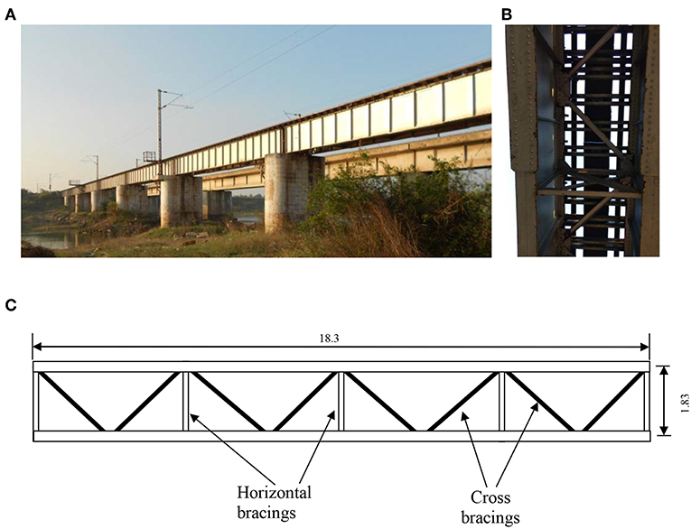
Figure 1. Ponneri railway bridge. (A) Photo of the bridge. (B) View from bottom. (C) Plan.

The first span of the bridge was instrumented with 16 strain gauges and 8 accelerometers as shown in Figure 2. Accelerometers are fixed at the mid span as well as on either sides, 4.6 m from the supports. Locations 1 and 2 have 3 accelerometers each, taking measurements in X, Y and Z directions. Location 3 has 2 accelerometers in the X and Y directions. Stain gauges are fixed on the top of the bottom flange and bottom of the top flange at an interval of 2.25 m along the span. All the sensors are installed on the exterior face of the outer girder where access was available. The strain gauges are numbered from S1 to S16, out of which S1–S8 are installed at the top and S9–S16 at the bottom. S1 (top) and S16 (bottom) are near the first support. The remaining sensors are numbered sequentially from this end. HBM QuantumX is used for data acquisition with a sampling frequency of 600 Hz.

FIGURE 2

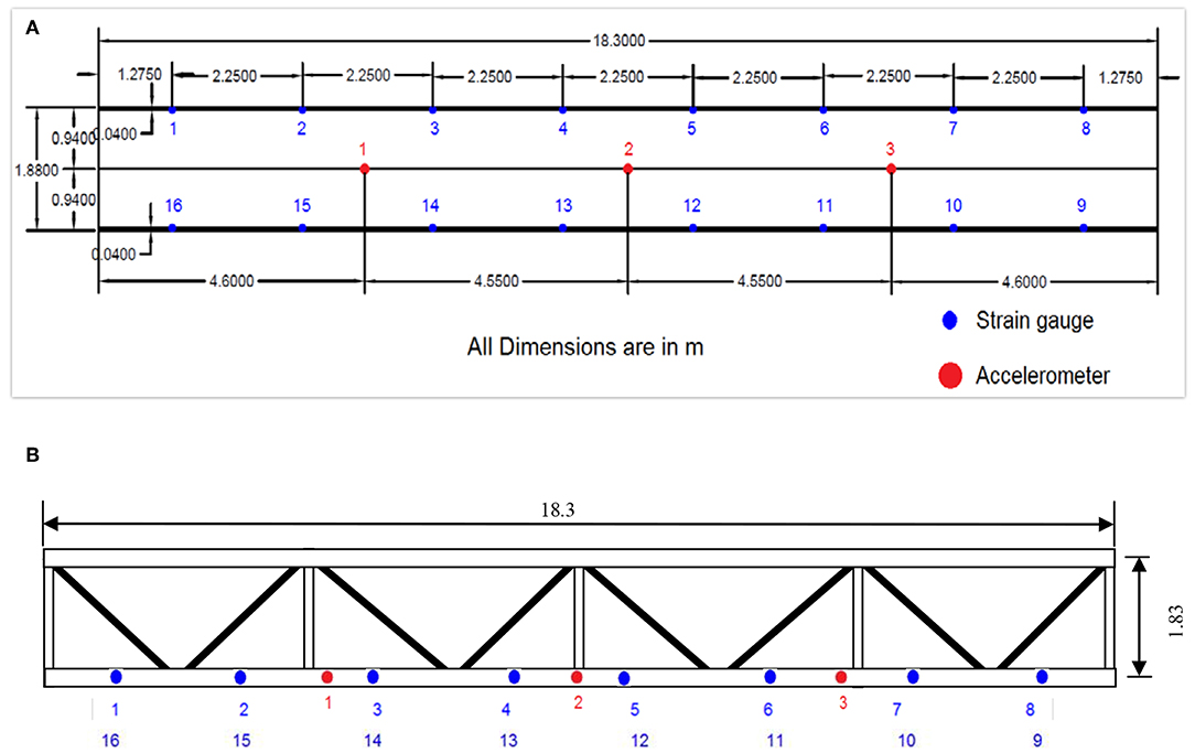
Figure 2. Ponneri railway bridge instrumentation. (A) Elevation. (B) Plan view (sensors are on the exterior face of the outer girder).

Trial runs were conducted after instrumentation. The main data collection was performed continuously for 10 h. During this period 31 trains crossed the bridge including 11 express trains. The measurements were started whenever the train is seen approaching the bridge. Tests were planned based on the schedule of trains given by the office of Chief Bridge Engineer, Southern Railways.

Analysis of strain data collected for one express train is presented in this paper. Similar conclusions are obtained for all other trains. The measurements during three stages were extracted, (a) during the free vibrations while the train is approaching the bridge (at this time, the train is still not on the instrumented span) (b) while the train is actually on the instrumented span c) while the train has left the span.

Visualization Tool

A tool called RRPExplorer (http://www.bennyraphael.com/RRPX/index.html) was used for visually navigating through the multi-dimensional data and extracting patterns in data. The tool uses the concept of parallel axis plots for analyzing trends in data (see section Visual Data Interpretation). The concept of multi-dimensional navigation using parallel axis plots has been used for tasks such as multi-criteria decision making (Raphael, 2011) and HVAC design (Pantelic et al., 2012).

Validation of Results

The data patterns obtained in the previous step are validated using quantitative methods. Statistical parameters such as correlation and degree of fit in multi-variate regression are used to confirm the findings.

Results

Challenges in Data Interpretation

If the geometry, material properties, support conditions and the load are known fairly accurately, the structure can be analyzed using finite element method and the structural responses can be compared with the measurements. However, in the present case, there are too many uncertainties. First of all, the load is unknown because the number of passengers in the train and the weight of the train cannot be estimated precisely. Secondly, it is not the case of simple static loading since the train moves over the track supported by many wheels. The train load acts on the bridge through a complex system consisting of rail track, rail pad, sleepers, ballast, fixtures, and fasteners. Due to the flexibility of the sleepers, there are vibrations on the track when the wheels move over it and there might be temporary loss of contact between the components. The resulting behavior may only be modeled as a dynamic system consisting of springs and masses. The stiffness of the springs and the masses affect the dynamic behavior and the damping parameters are not known. Transient structural analysis needs to be carried out to get the responses in this case involving forced vibrations. In order to compare sensor data with analysis results, relevant features need to be extracted from the time series of predicted and measured responses.

Initially, the bridge was modeled as a spring-mass system in which the vehicle and track-system was coupled (Das, 2018). The vehicle was modeled as a rigid body with 10° of freedom. The rail was modeled as a linear elastic Bernoulli–Euler beam with finite length, and the bridge decks were modeled as a series of multi-span continuous Bernoulli–Euler beams. The elasticity and damping properties of the rail bed were represented by continuous springs. Time history of strain values were obtained by simulating this model. The simulation results showed similar trends as that of real time field data, but the magnitude of strains were significantly different. The detailed dynamic model was not useful in providing definite conclusions about the state of the structure.

Another issue is the large amount of data to be analyzed (Omenzetter and Brownjohn, 2006), when there are multiple sensor locations and the sampling rate is high. It is difficult to assess how well simulations match measurements at all the time steps and sensor locations. Mean square error or similar metrics have been used to compare simulation results with measurements. These metrics convert data at multiple locations and time into a single number, and is convenient for assessing the degree of match. However, information about the trends and patterns in data are lost in the process. Even though, data mining techniques have been used to extract patterns in data, there are many proposals and choosing the best methods for a particular application is not easy.

Visual Data Interpretation

A convenient method of visualizing multi-dimensional data is through parallel axis plots (Raphael, 2011). In a parallel axis plot, each variable is represented by a vertical axis, and each value of the variable by a point on this axis. A given data point consists of a set of values for each variable and this is represented by a series of straight lines connecting the vertical axes. In Figure 3A, the vertical lines represent the strain values from sensors S1, S16, S2, etc. The axes are arranged such that sensors at the top and bottom of the girder, at the same longitudinal distance, are adjacent. The last axis represents the time at which the data is recorded. Three data points P1, P2, and P3 are shown as lines having different colors. These represent strain readings recorded at three different times. This form of representation helps to understand patterns in the data. For example, it can be seen that all the sensors have low values at time 3.02 s, and they have maximum values at time 3.47 s. The sensor values more or less increase or decrease together.

FIGURE 3

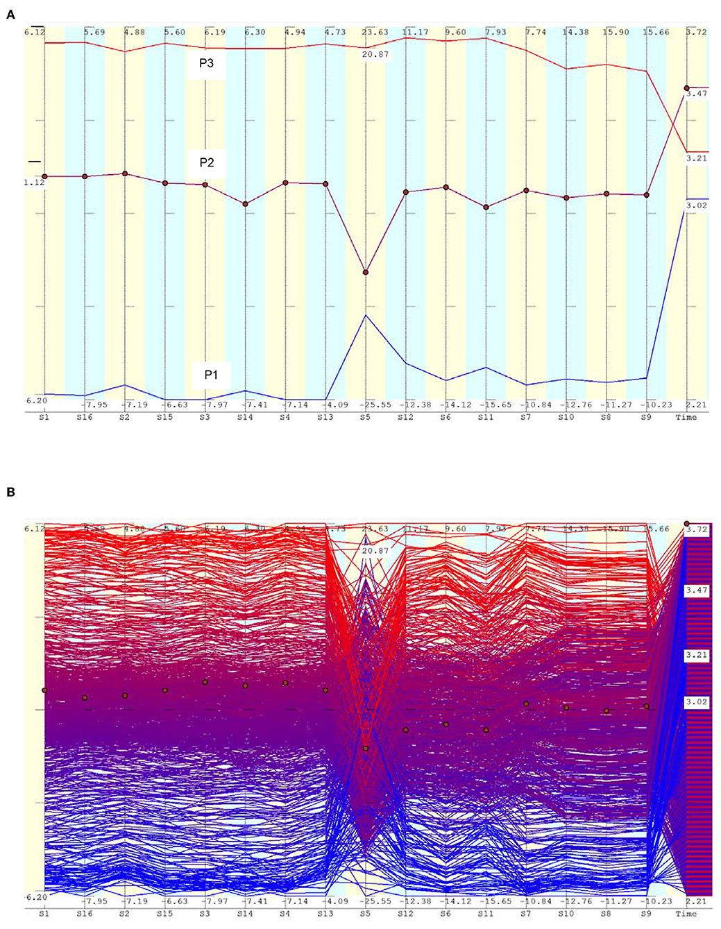
Figure 3. Parallel axis plot of strain data during the free vibration phase. (A) Plot of three data points to show the trend. These data belong to the free vibration period, when the train is far away from the span, roughly 986 m from the edge of the girder. The train was moving at a speed of 17.3 m/s. (B) Data points within a selected time frame.

Figure 3B shows more data points. These correspond to the strain readings recorded while a train was approaching the bridge from a distance, that is, the free vibrations induced on the bridge when the train load was not actually on the bridge. The series of parallel lines indicate that most sensor values increase or decrease together, that is, they are correlated. Sensor S5 is an exception which breaks the trend. Very often, S5 has low values when other sensors have large values, which is indicated by the lines crossing each other in the neighborhood of this axis.

Visual inspection of the data using parallel axis plot revealed two crucial points.

1) Sensors at the top and bottom are either in tension or compression at the same time. This is not possible using the simple model of the bridge girder as a simply supported beam bending about its principal axis (transverse horizontal axis).

2) Sensor S5, which is near the mid-span, undergoes local vibrations and is not in sync with the other sensors.

The patterns in data were totally unexpected and did not conform to the initial intuitive model of a simply supported girder. The only explanation for point 1 is that the bridge undergoes predominantly transverse vibrations, instead of vertical vibrations. Only in the case of transverse vibrations, it is possible to have the same sign of stress at the top and bottom.

The second observation is equally important. It indicates that the bridge girder cannot be modeled as a simply supported beam and certain details near the mid span induces local vibrations in that region. Parallel axis plot helps in visually navigating through the solution space by selecting regions of interest. Contiguous or separated parts of the space can be selected for closer examination by choosing windows with a pointing device. This helps in studying patterns within selected regions. In Figure 4A, data points having large negative values for sensor S5 are selected. These points have high positive values for other sensors. Similarly points having high positive values for sensor S5 are selected in Figure 4B. Most other sensors have negative values for these points. This confirms that there are strong local vibrations near the mid span.

FIGURE 4

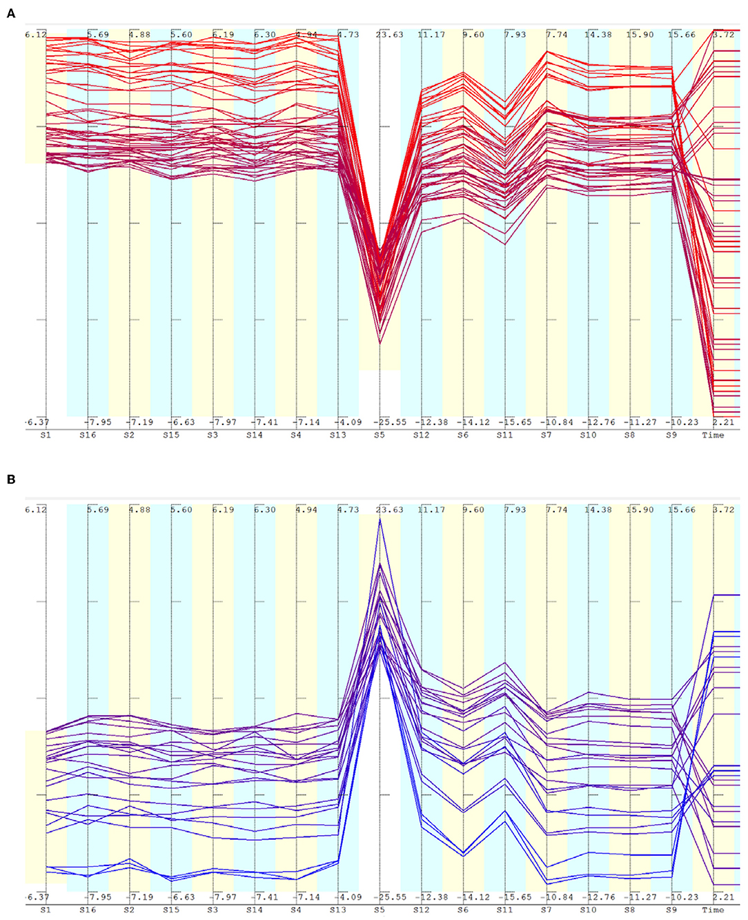
Figure 4. Parallel axis plot of selected strain data during the free vibration phase. (A) Selected data points with low values for sensor S5. (B) Selected data points with high values for sensor S5.

Closer examination revealed that the girder is spliced at the mid span using riveted connections (see Figure 5) and there are cross bracings near the mid span acting like local supports for the mid part of the girder, during transverse vibrations. This causes the middle part of the beam to vibrate locally between the local supports. In Figure 1B, the cross bracings connecting the top flanges of the two I sections of the bridge can be clearly seen. There is a possibility of local vibrations if the rivets on the particular cross bracings near the strain gauge 5 are loose. This might be a plausible explanation for the abnormal trend in the strain gauge 5. The adjacent sensors need not show the same results if the remaining cross bracings have sufficient stiffness and have no defects. Soon after the measurements, rivets were tested and about 40 loose rivets, distributed throughout the span, were replaced. The loose rivets have been identified as the cause of strong local vibrations. Since the railway authorities had given permission to carry out the experiments during a narrow window of 3 days, due to the heavy traffic on the line, measurements could not be repeated after the rivets were replaced. However, the engineers have remarked that after the fix, they now feel lighter vibrations while standing on the refuge platform on the bridge while trains pass by.

FIGURE 5

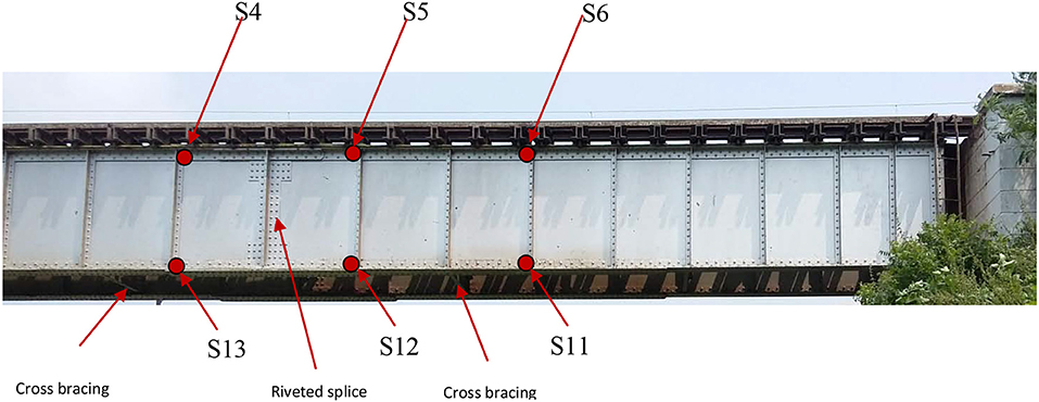
Figure 5. Ponneri bridge—connection details.

The dynamic behavior described so far is valid only during the period when the train is on the adjacent span. When the train enters the span, the vibration patterns change to predominantly vertical vibrations. The heavy load of the train and its impact tend to suppress the transverse vibrations. Data taken when the train is moving on the span is shown in Figure 6A. Inverse correlation between sensors at the top and bottom are visible through the lines that cross from large positive regions to large negative regions of the adjacent axis. This is more prominently visible in Figure 6B in which middle part of sensor S4 is removed. Even in this case, it can be seen that the sensor S5 has a different pattern than S2, S3, and S4.

FIGURE 6

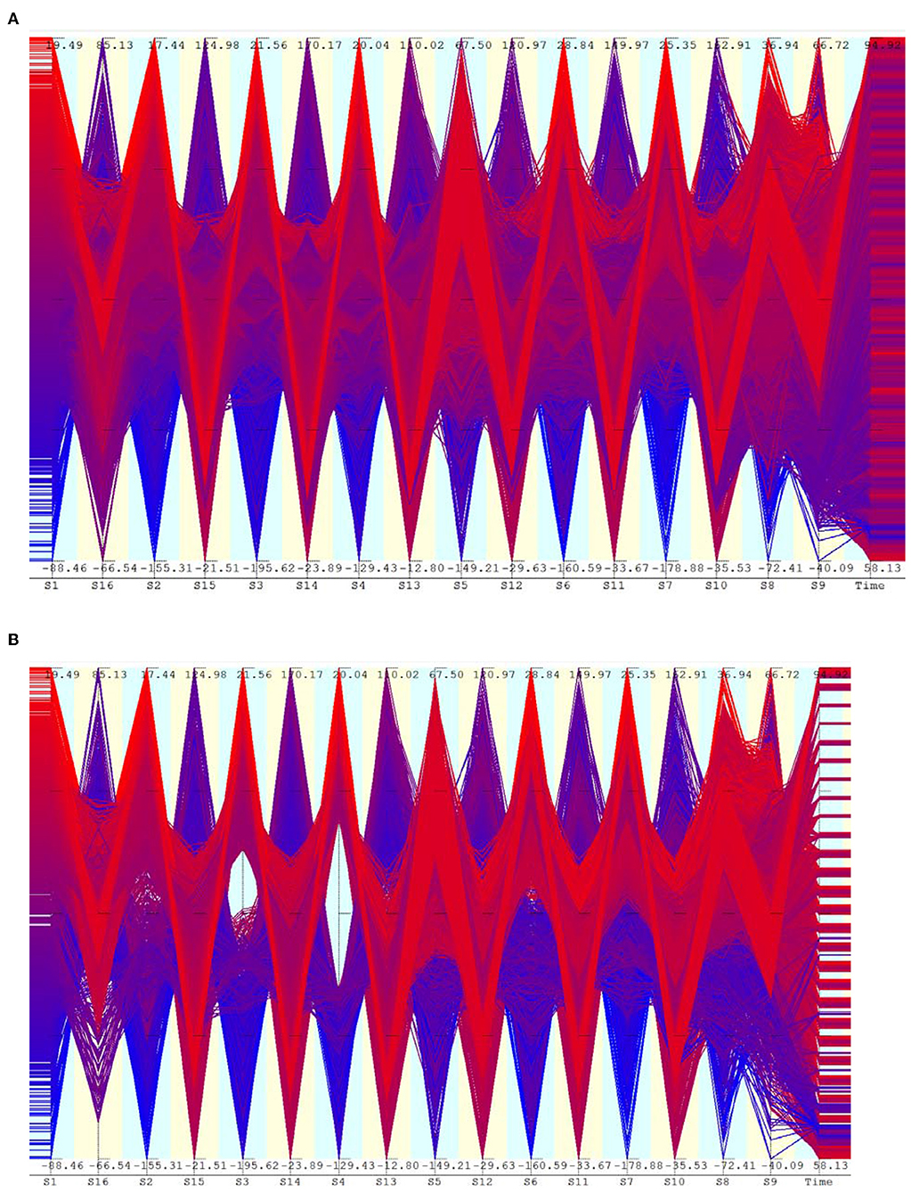
Figure 6. Parallel axis plot of strain data when the train is on the span. (A) Strain at around recording time 58.1 s, when the front of the train is at the edge of the girder. (B) Selected data points having high and low values of sensor S4.

The possible explanation that the abnormal readings of sensor S5 might be due to defect in the sensor itself is categorically ruled out. All the sensors were carefully calibrated and checked after the installation. Under heavy train loads, the maximum strains recorded by S4 and S5 are very close. Under free vibration conditions, the sensor S5 produce values that oscillate around a mean value close to zero. Under forced vibration conditions (when train is on the span), the values of S5 oscillate around a mean negative value as expected. The strain patterns just before and after the train enters the span are compared with accelerometer readings at the mid-span to check whether the trends are similar. In Figure 7A, the accelerometer readings show large amplifications around 58.8 s when the train enters the span. In Figure 7B, it can be seen that strain values start recording high negative values around the same time.

FIGURE 7

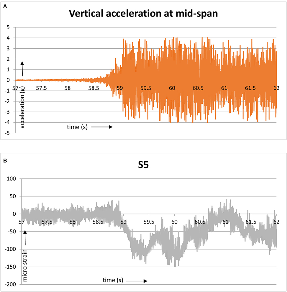
Figure 7. Sensor readings at the mid-span when the train enters the span. (A) Vertical acceleration. (B) Longitudinal strain.

The out-of-sync vibrations recorded by sensor S5 are confirmed by the accelerometer readings as well. During the free vibration phase, the transverse acceleration at the mid-span is of the same order of magnitude as the vertical acceleration. Also, high absolute values of transverse acceleration at the mid-span correspond to relatively low values on either side. Figure 8 shows the parallel axis plot of accelerometer readings at locations 1 and 2. The accelerometer 2 is at the mid-span. In order to reduce clutter, not all readings are shown; only accelerations in the vertical and transverse directions (z and y) are shown. Readings having high absolute values for accelerometer 2 are shown in the plot. The lines going down from the first axis to the second correspond to data points that have high values for the vertical acceleration at 2 and relatively low values at 1. If the vibrations at these two locations were synchronous, we should see parallel lines connecting these two axes. Similarly, the vertical accelerations are also not entirely synchronized. Examining the time axis, it is noted that the selected points with high absolute transverse accelerations are fairly uniformly distributed over time. This means that the vibrations have reasonable regularity with well defined frequencies.

FIGURE 8

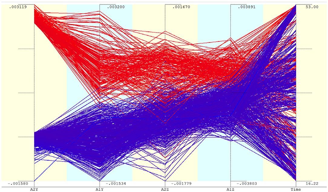
Figure 8. Selected accelerometer readings during the free-vibration phase. Only points with large absolute values of A2Y are chosen for display. During the selected time period, the train is at a distance of 735–98 m from the edge of the girder.

Analysis of data after the train has left the span yielded the same conclusions as that of the free vibration phase before the train reached the span. The anomaly in the strain patterns at S5 was equally pronounced in this stage as well. This is shown in Figure 9. Comparing this with Figure 4A, similar trends can be identified.

FIGURE 9

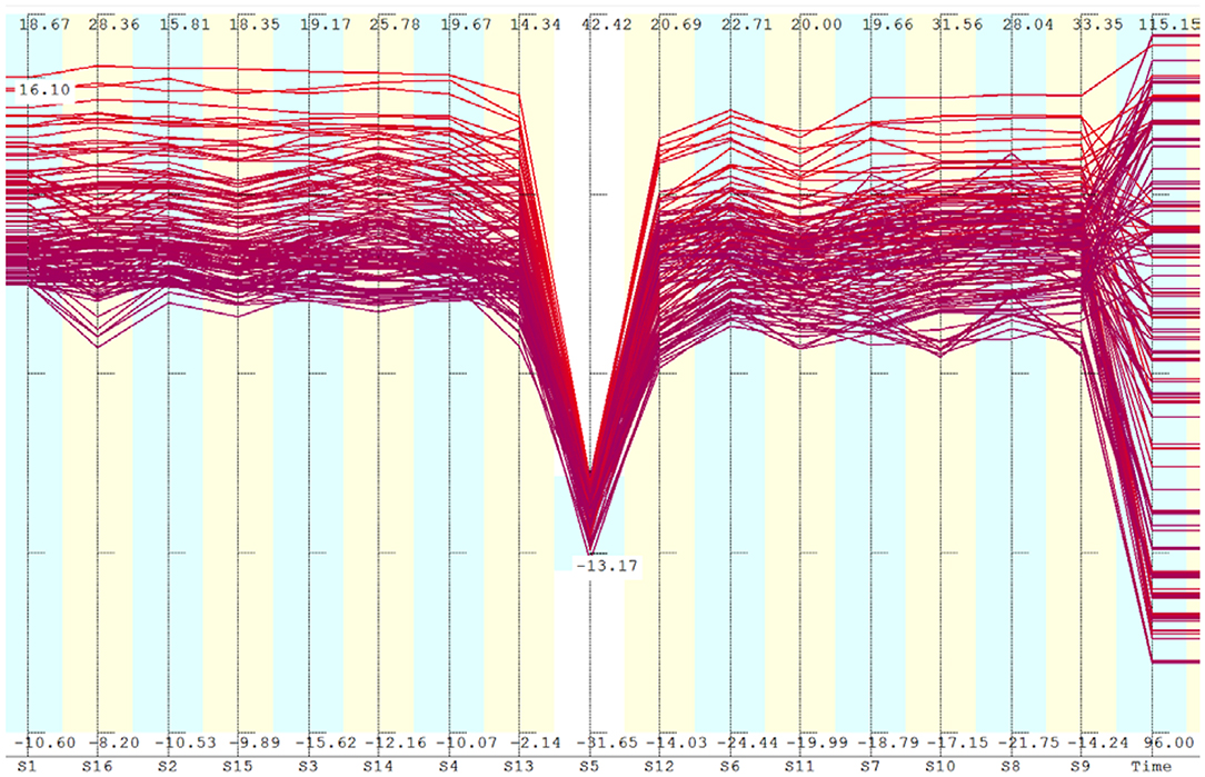
Figure 9. Free vibrations after the train has left the span. Only points having large negative value of S5 are shown. Comparing with Figure 4A, similar patterns are identified.

Confirmation of Visual Observations

Quantitative statistical methods were used to confirm the findings from visual observations. Part of the correlation matrix of sensor values are shown in Table 1, for the data shown in Figure 3A (free vibrations when the train is approaching). It is seen that the sensors S1, S2, S3, and S6 are strongly correlated. Sensor S5 does not have good correlation with any other sensors.

TABLE 1

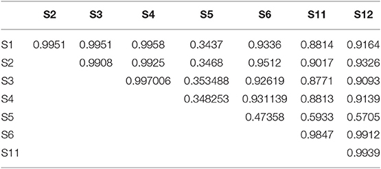
Table 1. Correlation of sensors when the train is on adjacent span.

The correlation between sensors at the bottom of the girder, when the train is on the span is shown in Table 2. Even though S5 is still weakly correlated with other sensors, the correlation coefficients have increased compared to Table 1. This is because the forced vibrations are causing the mid span to move in sync with other regions, even though, local transverse vibration modes are still present. The correlation of S6 with S1 is also relatively low. In fact, S6 has relatively high correlation with S5. A likely explanation is that the location of S6 is also slightly affected by the transverse vibration at S5.

TABLE 2

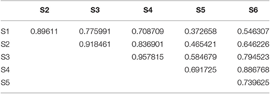
Table 2. Correlation of sensors when the train is on the selected span.

The correlation between sensors at the top and bottom for the case of forced vibrations are shown in Table 3. All these sensors show negative correlation, meaning that, when the top is in compression, the bottom is in tension and vice versa. Sensor S5 has relatively weak correlation with its counterpart at the top. This is because of local vibration component at S5, in addition to the vertical vibrations.

TABLE 3

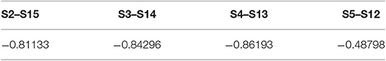
Table 3. Correlation between sensors at the top and bottom when the train is on the selected span.

Multi-variate regression was performed in order to find out whether sensor data at S5 is related to any other combination of sensors. It is emphasized that the purpose of regression is not to predict the value of S5. It is to check whether the readings from S5 is a linear combination of other sensor readings. That is, to find out which combination of sensors strongly determine the values of S5. This gives an indication of the vibration modes. Pair-wise correlation coefficients do not give this information. Here, the aim is to select a minimal set of sensors that mostly explain the data from S5. This is done using the following algorithm:

Step 1: Start with the number of independent regression variables n=0. The selected list of variables is empty to start with.

Step 2: Repeat for each variable, i, that is not yet included in the selected list

Step 2.1: Perform a regression with (n+1) independent variables, consisting of variable i and other variables in the current selected list. Calculate the degree of fit R.

Step 2.2: Keep track of the variable i that causes the largest increase in R

Step 3: If the R value has improved beyond a threshold (0.02), add the variable having the highest R to the selected list of variables, increment n and repeat Step 2.

This procedure selects variables that have the highest influence on the output variable (S5). It should be noted that, if a certain variable is highly correlated with an already selected variable, it will never get selected because the degree of fit will not be improved. That is, the correlated variable is not able to explain the variability in data any more than the already selected variable. Important results for the case of free vibrations are summarized in Table 4. In Table 4, the first row does not give the highest fit according to the above algorithm, nevertheless, it is added to show the low degree of fit with adjacent sensors. Even though S5 is not strongly correlated with any sensors individually, by adding certain adjacent sensors to the regression equation, the degree of fit increases to 0.903. That is, the reading at S5 is a linear combination of the sensors in its neighborhood. The regression equation is needed to explain this.

TABLE 4

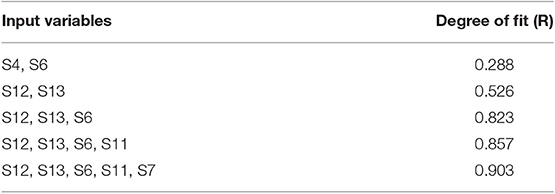
Table 4. Regression with S5 as the output variable.

The final regression equation is given by Equation (1). From the regression coefficients, it is noted that, on average, S5 moves in the opposite direction as the neighboring sensors at the top, S6 and S7. This happens when there are local vibrations between S6 and S7. Furthermore, the coefficients of S13 and S11 are positive, which indicates predominantly transverse vibrations (both top and bottom have the same sign of strain).

$\begin{array}{l}S5=3.815^{*}S13+0.848^{*}S12\text{-}3.708^{*}S6+7.395^{*}S11\\ \hfill \text{-}5.287^{*}S7+8.915& (1)\end{array}$

This is qualitatively explained as follows: During certain time steps (roughly 52% of the time), S5 is moving in sync with the neighboring sensors at the bottom, S12 and S13. This corresponds to predominantly transverse vibrations. At other time steps, S5 moves in the opposite direction as S6 and S7 (with negative correlation). This is when the local vibration dominates the transverse vibration.

Discussion

The primary objective of this paper is to illustrate the importance of visualization in understanding trends and patterns in data. Parallel axis plot is a convenient representation for multi-dimensional data that aids in highlighting important relationships between variables. In this representation, strongly correlated variables are indicated by parallel lines. Variables that break the trend can be detected by the presence of lines that criss-cross each other. This is clearly visible in the case of readings of sensor S5 (Figure 3B).

The parallel axis plot permits analyzing subsets of data by selecting windows along specific axes. This helps to reveal patterns within data contained in specific regions satisfying certain conditions. For example, by selecting large negative values for Sensor S5 (for the selected time window when the train is not on the current span), it is seen that the points are more or less uniformly distributed along the time axis (Figure 4A). This means that large negative strain is obtained at regular intervals, indicating that the girder is undergoing vibrations with a fairly well-defined time period. During these moments of high negative strain for S5, all the other sensors have mostly positive values, showing that the sensor S5 is vibrating in the opposite direction compared to other locations.

By selecting the time window when the train is actually on the span, definite patterns are found, which indicate predominantly vertical vibrations (Figures 6A,B). Even here, mixture of vibration modes are visible through a number of data points that connect large absolute values of some sensors to low values of other sensors.

Having identified the patterns described above, it is possible to perform specific statistical analysis to confirm the findings. The abnormal vibrations of sensor S5 was confirmed by its low correlation with other sensors. Mixture of modes of vibrations is confirmed by multi-variate linear regression which established that sensor S5 moves partly in sync with S11, S12, and S13, and out of sync with S6 and S7.

The insights obtained by visual analysis and confirmed by statistical analysis, provides clues to accurately modeling the structure for applying more sophisticated quantitative methods such as system identification. The data patterns made it clear that the girders might not be modeled as simply supported beams; riveted splices at the mid-span and the cross bracings are important in numerically reproducing the transverse and local vibrations near the mid-span. Detailed numerical modeling of the bridge is out of scope of this paper.

Summary and Conclusions

A relatively simple bridge girder exhibits complex vibration patterns that were not intuitively expected. The mode of vibration changes significantly when the train is actually on the bridge compared to the free vibrations induced when the train is approaching from the neighboring span. The complex behavior of the bridge is primarily because of defective connections (loose rivets). This demonstrates the complexities in the condition assessment of structures. Even when the normal design models of the bridge are simple, actual as-built conditions might be very complex. Population based system identification methods are useful in such cases. Many instances consisting of normal models and fault models are necessary in order to explain the sensor data. However, qualitative understanding of the patterns in the data is necessary even for developing plausible model classes. Otherwise, critical aspects of the structural behavior might not be incorporated in the model class. Visual analysis of data helps in this task, as illustrated using the case study in this paper.

The limitations of the present study include the following:

• Complex statistical analysis methods have not been used to extract data patterns. Only correlation coefficients are computed in this study. Visual examination indicates that clustering techniques might be useful, but this has not been attempted.

• Spectral analysis of the measurement data is not reported here. Frequencies extracted through Fast Fourier Transform (FFT) show interesting patterns. This is work in progress.

Data Availability Statement

The datasets generated for this study are available on request to the corresponding author.

Author Contributions

AH performed the research under the supervision of BR.

Conflict of Interest

The authors declare that the research was conducted in the absence of any commercial or financial relationships that could be construed as a potential conflict of interest.

Acknowledgments

The doctoral research of AH was supported by the scholarship from Ministry of Human Resource Development (MHRD), India and Curtin International Postgraduate Research Scholarship (CIPRS), and Research Stipend Scholarship from Curtin University, Australia. The funding for instrumentation of the bridge from the Future Cities Lab Singapore is gratefully acknowledged. The authors wish to thank the Chief Bridge Engineer, Southern Railways, India for the permission and arrangements for the instrumentation.

References

Adeli, H., and Karim, A. (2000). Fuzzy-wavelet Rbfnn model for freeway incident detection. J. Transport. Eng. 126, 464–471. doi: 10.1061/(ASCE)0733-947X(2000)126:6(464)

CrossRef Full Text | Google Scholar

An, Y., Chatzi, E., Sim, S.-H., Laflamme, S., Blachowski, B., and Ou, J. (2019). Recent progress and future trends on damage identification methods for bridge structures. Struct. Control Health Monitor. (2019) 26, 1–30. doi: 10.1002/stc.2416

CrossRef Full Text | Google Scholar

Beck, J. L. (2010). Bayesian system identification based on probability logic. Struct. Control Health Monitor. 17, 825–847. doi: 10.1002/stc.424

CrossRef Full Text | Google Scholar

Beck, J. L., and Katafygiotis, L. S. (1998). Updating models and their uncertainties. I: Bayesian statistical framework. J. Eng. Mech. 124, 455–461.

Google Scholar

Ben-Haim, Y., and Hemez, F. M. (2012). Robustness, fidelity and prediction-looseness of models. Proc. R. Soc. A Math. Phys. Eng. Sci. 468, 227–244. doi: 10.1098/rspa.2011.0050

CrossRef Full Text | Google Scholar

Berger, J. O., and Pericchi, L. R. (1996). The intrinsic bayes factor for model selection and prediction. J. Am. Stat. Assoc. 91, 109–122. doi: 10.1080/01621459.1996.10476668

CrossRef Full Text | Google Scholar

Beven, K. (2009). Environmental Modelling: An Uncertain Future? Routledge; Taylor & Francis Group. Available online at: http://books.google.dk/books/about/Environmental_Modelling.html?id=A_YXIAAACAAJ&pgis=1

Google Scholar

Beven, K. J. (2000). Uniqueness of place and process representations in hydrological modelling. Hydrol. Earth Syst. Sci. 4, 203–213. doi: 10.5194/hess-4-203-2000

CrossRef Full Text | Google Scholar

Brownjohn, J. M. W., Xu, Y., and Hester, D. (2017). Vision-based bridge deformation monitoring. Front. Built Environ. 3:23. doi: 10.3389/fbuil.2017.00023

CrossRef Full Text | Google Scholar

Catbas, F. N., and Malekzadeh, M. (2016). A machine learning-based algorithm for processing massive data collected from the mechanical components of movable bridges. Autom. Constr. 72, 269–278. doi: 10.1016/j.autcon.2016.02.008

CrossRef Full Text | Google Scholar

Cavadas, F., Smith, I. F. C., and Figueiras, J. (2013). Damage detection using data-driven methods applied to moving-load responses. Mech. Syst. Signal Process. 39, 409–425. doi: 10.1016/j.ymssp.2013.02.019

CrossRef Full Text | Google Scholar

Chouinard, L., Shahsavari, V., and Bastien, J. (2019). Reliability of wavelet analysis of mode shapes for the early detection of damage in beams. Front. Built Environ. 5:91. doi: 10.3389/fbuil.2019.00091

CrossRef Full Text | Google Scholar

Das, S. (2018). Dynamic Interaction of Train-Track-Bridge System. Master's Thesis, Indian Institute of Technology Madras, Chennai, India.

Google Scholar

Feng, D., and Feng, M. Q. (2018). Computer vision for SHM of civil infrastructure: from dynamic response measurement to damage detection – a review. Eng. Struct. 156, 105–117. doi: 10.1016/j.engstruct.2017.11.018

CrossRef Full Text | Google Scholar

Ghosh, B., Basu, B., and O'Mahony, M. (2010). Random process model for urban traffic flow using a wavelet-bayesian hierarchical technique. Comput. Aided Civil Infrastruct. Eng. 25, 613–624. doi: 10.1111/j.1467-8667.2010.00681.x

CrossRef Full Text | Google Scholar

Glisic, B., Yarnold, M. T., Moon, F. L., and Aktan, A. E. (2014). Advanced visualization and accessibility to heterogeneous monitoring data. Comput. Aided Civil Infrastruct. Eng. 29, 382–398. doi: 10.1111/mice.12060

CrossRef Full Text | Google Scholar

Goller, B., Beck, J. L., and Schuëller, G. I. (2012). Evidence-based identification of weighting factors in bayesian model updating using modal data. J. Eng. Mech. 138, 430–440. doi: 10.1061/(ASCE)EM.1943-7889.0000351

CrossRef Full Text | Google Scholar

Goulet, J.-A. (2012). Probabilistic Model Falsification for Infrastructure Diagnosis. Doctoral Thesis, École Polytechnique Fédérale de Lausanne, Lausanne, Switzerland.

Google Scholar

Goulet, J.-A., Coutu, S., and Smith, I. F. C. (2013a). Model falsification diagnosis and sensor placement for leak detection in pressurized pipe networks. Adv. Eng. Informatics 27, 261–269. doi: 10.1016/j.aei.2013.01.001

CrossRef Full Text | Google Scholar

Goulet, J.-A., Michel, C., and Smith, I. F. C. (2013b). Hybrid probabilities and error-domain structural identification using ambient vibration monitoring. Mech. Syst. Signal Process. 37, 199–212. doi: 10.1016/j.ymssp.2012.05.017

CrossRef Full Text | Google Scholar

Harichandran, A., Raphael, B., and Mukherjee, A. (2019). “Identification of the structural state in automated modular construction,” 36th International Symposium on Automation and Robotics in Construction (ISARC 2019) (Banff, AB), 187–193.

Google Scholar

He, W.-Y., Zhu, S., and Ren, W.-X. (2019). Two-phase damage detection of beam structures under moving load using multi-scale wavelet signal processing and wavelet finite element model. Appl. Math. Model. 66, 728–744. doi: 10.1016/j.apm.2018.10.005

CrossRef Full Text | Google Scholar

Huang, C. S., Hung, S. L., Wen, C. M., and Tu, T. T. (2003). A neural network approach for structural identification and diagnosis of a building from seismic response data. Earthq. Eng. Struct. Dyn. 32, 187–206. doi: 10.1002/eqe.219

CrossRef Full Text | Google Scholar

Jeffreys, H. (1998). Theory of Probability. Available online at: https://global.oup.com/academic/product/the-theory-of-probability-9780198503682?cc=in&lang=en&

Google Scholar

Jiang, X., and Adeli, H. (2003). Fuzzy clustering approach for accurate embedding dimension identification in chaotic time series. Integr. Comput. Aided Eng. 10, 287–302. doi: 10.3233/ICA-2003-10305

CrossRef Full Text | Google Scholar

Kromanis, R., and Kripakaran, P. (2017). Data-driven approaches for measurement interpretation: analysing integrated thermal and vehicular response in bridge structural health monitoring. Adv. Eng. Informatics 34, 46–59. doi: 10.1016/j.aei.2017.09.002

CrossRef Full Text | Google Scholar

Li, H., Huang, Y., Chen, W. L., Ma, M. L., Tao, D. W., and Ou, J. P. (2011). Estimation and warning of fatigue damage of FRP stay cables based on acoustic emission techniques and fractal theory. Comput. Aided Civil Infrastruct. Eng. 26, 500–512. doi: 10.1111/j.1467-8667.2010.00713.x

CrossRef Full Text | Google Scholar

Moreu, F., Li, X., Li, S., and Zhang, D. (2018). Technical specifications of structural health monitoring for highway bridges: new chinese structural health monitoring code. Front. Built Environ. 4:10. doi: 10.3389/fbuil.2018.00010

CrossRef Full Text | Google Scholar

Mottershead, J. E., Link, M., and Friswell, M. I. (2011). The sensitivity method in finite element model updating: a tutorial. Mech. Syst. Signal Process, 25, 2275–2296. doi: 10.1016/j.ymssp.2010.10.012

CrossRef Full Text | Google Scholar

Napolitano, R., Liu, Z., Sun, C., and Glisic, B. (2019). Combination of image-based documentation and augmented reality for structural health monitoring and building pathology. Front. Built Environ. 5:50. doi: 10.3389/fbuil.2019.00050

CrossRef Full Text | Google Scholar

Ngeljaratan, L., and Moustafa, M. A. (2019). System identification of large-scale bridges using target-tracking digital image correlation. Front. Built Environ. 5:85. doi: 10.3389/fbuil.2019.00085

CrossRef Full Text | Google Scholar

Omenzetter, P., and Brownjohn, J. M. W. (2006). Application of time series analysis for bridge monitoring. Smart Mater. Struct. 15, 129–138. doi: 10.1088/0964-1726/15/1/041

CrossRef Full Text | Google Scholar

Pai, S. G. S., Nussbaumer, A., and Smith, I. F. C. (2018). Comparing structural identification methodologies for fatigue life prediction of a highway bridge. Front. Built Environ. 3:73. doi: 10.3389/fbuil.2017.00073

CrossRef Full Text | Google Scholar

Pan, S., Xu, S., Mirshekari, M., Zhang, P., and Noh, H. Y. (2017). Collaboratively adaptive vibration sensing system for high-fidelity monitoring of structural responses induced by pedestrians. Front. Built Environ. 3:28. doi: 10.3389/fbuil.2017.00028

CrossRef Full Text | Google Scholar

Pantelic, J., Raphael, B., and Tham, K. W. (2012). A preference driven multi-criteria optimization tool for HVAC design and operation. Energy Build. 55, 118–126. doi: 10.1016/j.enbuild.2012.04.021

CrossRef Full Text | Google Scholar

Papadopoulou, M., Raphael, B., Smith, I. F. C., and Sekhar, C. (2014). Hierarchical sensor placement using joint entropy and the effect of modeling error. Entropy 16, 5078–5101. doi: 10.3390/e16095078

CrossRef Full Text | Google Scholar

Pasquier, R., and Smith, I. F. C. (2015). Robust system identification and model predictions in the presence of systematic uncertainty. Adv. Eng. Informatics 29, 1096–1109. doi: 10.1016/j.aei.2015.07.007

CrossRef Full Text | Google Scholar

Posenato, D., Kripakaran, P., Inaudi, D., and Smith, I. F. C. (2010). Methodologies for model-free data interpretation of civil engineering structures. Comput. Struct. 88, 467–482. doi: 10.1016/j.compstruc.2010.01.001

CrossRef Full Text | Google Scholar

Poston, J. D., Buehrer, R. M., and Tarazaga, P. A. (2017). A framework for occupancy tracking in a building via structural dynamics sensing of footstep vibrations. Front. Built Environ. 3:65. doi: 10.3389/fbuil.2017.00065

CrossRef Full Text | Google Scholar

Raphael, B. (2011). Multi-criteria decision making for collaborative design optimization of buildings. Built Environ. Project Asset Manage. 1, 122–136. doi: 10.1108/20441241111180398

CrossRef Full Text | Google Scholar

Raphael, B., and Smith, I. F. C. (2013). Engineering Informatics – Fundamentals of Computer-Aided Engineering. Chichester: John Wiley.

Google Scholar

Robert-Nicoud, Y., Raphael, B., Burdet, O., and Smith, I. F. C. (2005a). Model identification of bridges using measurement data. Comput. Aided Civil Infrastruct. Eng. 20, 118–131. doi: 10.1111/j.1467-8667.2005.00381.x

CrossRef Full Text | Google Scholar

Robert-Nicoud, Y., Raphael, B., and Smith, I. F. (2005b). System identification through model composition and stochastic search. J. Comput. Civil Eng. 19, 239–247. doi: 10.1061/(ASCE)0887-3801(2005)19:3(239)

CrossRef Full Text | Google Scholar

Schoefs, F., Yáñez-Godoy, H., and Lanata, F. (2011). Polynomial chaos representation for identification of mechanical characteristics of instrumented structures. Comput. Aided Civil Infrastruct. Eng. 26, 173–189. doi: 10.1111/j.1467-8667.2010.00683.x

CrossRef Full Text | Google Scholar

Sirca, G. F., and Adeli, H. (2012). System identification in structural engineering. Sci. Iranica 19, 1355–1364. doi: 10.1016/j.scient.2012.09.002

CrossRef Full Text | Google Scholar

Soman, R. K., Raphael, B., and Varghese, K. (2017). A system identification methodology to monitor construction activities using structural responses. Autom. Constr. 75, 79–90. doi: 10.1016/j.autcon.2016.12.006

CrossRef Full Text | Google Scholar

Vernay, D. G., Raphael, B., and Smith, I. F. C. (2015). A model-based data-interpretation framework for improving wind predictions around buildings. J. Wind Eng. Indus. Aerodyn. 145, 219–228. doi: 10.1016/j.jweia.2015.06.016

CrossRef Full Text | Google Scholar

Yu, W., and Li, X. (2010). Automated nonlinear system modeling with multiple fuzzy neural networks and kernel smoothing. Int. J. Neural Syst. 20, 429–435. doi: 10.1142/S0129065710002516

PubMed Abstract | CrossRef Full Text | Google Scholar

Zhou, Q., and Yu, T. X. (2004). Use of high-efficiency energy absorbing device to arrest progressive collapse of tall building. J. Eng. Mech. 130, 1177–1187. doi: 10.1061/(ASCE)0733-9399(2004)130:10(1177)

CrossRef Full Text | Google Scholar

Zhu, Y., Ni, Y.-Q., Jin, H., Inaudi, D., and Laory, I. (2019). A temperature-driven MPCA method for structural anomaly detection. Eng. Struct. 190, 447–458. doi: 10.1016/j.engstruct.2019.04.004

CrossRef Full Text | Google Scholar

Zonta, D., Glisic, B., and Adriaenssens, S. (2014). Value of information: impact of monitoring on decision-making. Struct. Control Health Monitor. 21, 1043–1056. doi: 10.1002/stc.1631

CrossRef Full Text | Google Scholar