A Study of the Effects of Tornado Translation on Wind Loading Using a Potential Flow Model

1. Introduction

Tornadoes are one of the most devastating weather events due their violent wind speed and unpredictable nature. Each year more than 1,200 tornadoes are reported in the United States causing approximately 80 deaths, 1,500 injuries and more than $800 million worth of damage (NOAA, 2012). In 2011 alone, tornadoes claimed the lives of more than 500 people and caused $10 billion dollars in damage in the United States, according to the National Oceanic and Atmospheric Administration (NOAA, 2012). Therefore, the study on tornadoes has received growing attention in recent years with the desire to reduce the socio-economic losses that would occur in the event of such devastating weather events.

Due to the violent wind speed, unpredictable tracks and short warning lead time of only 10–15 min (Savory et al., 2001), direct measurements are not always possible and can be very dangerous. As a result, the modelling of tornadoes using analytical models, laboratory-scaled experiments and numerical simulation have been the alternatives to study the flow fields of tornado-like vortices. The earliest systematic attempt to experimentally study laboratory-scaled tornado-like vortices is frequently attributed to Ward (1972). Ward’s vortex simulator utilises an exhaust fan atop the simulator to provide the updraft flow and a number of guide vanes near the ground to generate the required angular momentum for the formation of the vortices. The study proposed that the radial momentum flux is one of the primary parameters sustaining the vortex flow structure and showed the reproduction of vortex evolution by adjusting the angular momentum. Following this, extensive studies using analytical models (Harlow and Stein, 1974; Jischke and Parang, 1974; Baker and Church, 1979; Rotunno 1979; Fiedler and Rotunno, 1986) and physical tornado simulators (Wan and Chang, 1972; Church et al., 1979; Mitsuta and Monji, 1984; Monji, 1985; Haan et al., 2008; Matsui and Tamura, 2009; Hashemi Tari et al., 2010; Refan et al., 2014; Gillmeier et al., 2017; Refan and Hangan, 2018; Ashton et al., 2019; Gillmeier et al., 2019; Ashrafi et al., 2021) as well as numerical simulators (Ishihara et al., 2011; Ishihara and Liu, 2014; Eguchi et al., 2018; Yuan et al., 2019; Gairola and Bitsuamlak, 2019; Kashefizadeh et al., 2019; Kawaguchi et al., 2019; Li et al., 2020) had been conducted in order to study the flow fields of tornado-like vortices. However, due to various constraints, these simulators cannot facilitate comprehensive study of vortex translation.

In recent years, large-scale translating experimental tornado simulators have been built to study tornado wind fields and the interactions with buildings. These include the tornado simulator at Iowa State University (Haan et al., 2008), which employs a unique top-down design, allowing for the generated vortex to translate along a ground plane to interact with building models and tornado induced loads of the structure to be quantified. Additionally, the WindEEE Dome, which is a relatively large-scale testing facility with a hexagonal wind chamber was also constructed at Western University (Hangan, 2014). With these facilities both experimental studies (Sarkar et al., 2006; Mishra et al., 2008; Mishra et al., 2008; Sabareesh et al., 2009; Zhang and Sarkar, 2012) and numerical studies (Sengupta et al., 2008; Natarajan and Hangan, 2012; Nasir and Bitsuamlak, 2016) were conducted to investigate the tornado-building interaction. While these large-scale tornado simulators have the ability to effectively model the translation of tornadoes, they are restricted to relatively slow translation speeds (0.5–2 m/s) and as such the relative speed of translation to that of the maximum tangential velocity speed is 0.014–0.16% (Razavi and Sarkar, 2018; Refan and Hangan, 2018). Moreover, while numerical simulation provides as an alternative to the physical simulations, the numerical models often require experimental results for validation (Gairola and Bitsuamlak, 2019). As a result, the effects of tornado translation speed, particularly higher translating speeds, on building aerodynamics is still not well understood.

Numerous studies have been conducted with the intention of quantifying the effects induced by tornadoes on a buildings; Mishra et al. (2008) compared the measurements on a cubic building model in a tornado-like vortex flow field and a boundary layer wind tunnel and concluded that the pressure and force on the building model exhibit different characteristics and outlined the need to further explore the tornado-building interaction and the wind loading. Haan et al. (2010) employed a gable-roof building model in the flow field of a translating vortex with varying translating velocities and swirl ratios and found that the maximum force coefficient on the build appears to decrease with the increase in translating velocity.Wang et al. (2018) found that the aerodynamic loads on a cubic building caused by tornado-like vortices resembles to those from boundary layer wind when the building is situated within the tornado core radius. Recently, Kopp and Wu (2020) presented a framework comparing the wind load on low-rise buildings in tornado-like wind field and in straight-line boundary layer wind. It was found that the swirling vortex flow created a lower pressure zone on the leeward walls of the building as well as altering the surface pressure distribution on the walls, resulting in a different vortex structure behind the building compared to the measurements from the boundary layer wind field. Razavi and Sarkar (2020) employed the ISU-type simulator to examine the effects of wind-induced uplift, shear and moment on roof geometries induced by the translating movement of tornadoes and found that ASCE 7-16 underestimates the overall uplift and moments. A study by Wang et al. (2021) reviewed the methods of simulating tornado wind fields in great detail and points out that the effects of tornado translation and the flow acceleration generated are crucial and may cause an increase or overshoot in the wind load. This overshoot phenomena was investigated by Takeuchi et al. (2008) by studying the effects of flow acceleration on an elliptic cylinder under short-rise-time gusts. It was reported that the inertial forces (force due to flow acceleration) greatly affected the occurrence of the overshoot phenomenon when the rise time is relatively small thus highlighting the potential additional effects tornado translation may have on buildings. According to ASCE 7-16 (2017), while the current design guideline for estimating wind loads on buildings in tornadoes are available, they are essentially based on wind loads in atmospheric boundary layers and does not actually account for any of the variability of the tornado flow field.

It is evident from the discussion above that the understanding of tornado-building interaction is still lacking. The effects of tornado translation speeds on the pressure distribution; hence, the overall force on buildings, still remains to be addressed.

The primary aim of this study is to explore the potential impact of tornado translation on the pressures and overall forces on a body. The second aim is to present a framework to reproduce the flow conditions and effects of the moving tornado. To achieve this, a vortex model describing the vortex movement was developed using unsteady potential flow theory; the model is simple but able to reproduce the flow conditions and summarise the characteristics of the phenomena. Then, the actual ranges of tornado translation speeds of naturally occurring tornadoes were assessed to determine the possible practical importance of these effects.

The subsequent sections are organised as follows: Section 2 outlines the development of the vortex model and explores the impact of tornado translation on the pressure field on a point and around an airfoil. Section 3 presents the relative range of translating speeds in naturally occurring tornadoes and finally, the application of methodology using the proposed expression for pressure adjustments and relative flow angles are discussed in section 4.

2. Translating Vortex

2.1 Vortex Translating Past a Point

In order to develop a vortex model able to describe the flow conditions and characteristics of a translating vortex, potential flow theory is used. Whilst it is acknowledged that this is a highly simplified approach, it does at least provide a scientifically robust framework in which to undertake the analysis. Additionally, within a tornado the inertial effects are likely to be significantly larger than the viscous effects and as such this approximation is likely to be sufficient (particularly for the purposes used below). The configuration considered is shown in Figure 1, which illustrates the 2D plan view of the ground plane of a fixed reference frame. The tornado is represented using a free vortex circulating in the anti-clockwise direction with the circulation strength of $\text{Γ}$ ($=2\pi r_c{V}_{\theta max}$, where $V_{\theta max}$ is the maximum tangential velocity of the vortex and $r_c$ is the radial distance which $V_{\theta max}$ occurs. NOTE: $r_c$ is an analytical convenience for this study and not actually a core radius. Since potential vortices do not have a finite core, an $r_c$ is merely used to define a circulation strength). The vortex translates in the direction parallel to the x-axis from $-x$ to + $x$ with the translating speed of $V_{trans}$. A body represented using a point, $B$, is placed at the origin at a distance of $r$ from the translating path of the vortex (Section 2.2 details further analysis using an airfoil to represent the body). Since the motion is assumed to be a free vortex flow (where tangential velocity is inversely proportional to the distance from the rotation axis), the tangential velocity at point $B$ will increase with a decrease in $r$. Additionally, if the body (point $B$, hereafter referred to as case 1) is placed at a distance of $+r$, the velocity induced by the vortex at point $B$ is greater (as $V_{\theta max}+V_{trans}$ due to the direction of vortex circulation), whereas, if placed at a distance of $-r$, the velocity at point $B$ is lower (as $V_{\theta max}-V_{trans}$). The potential function (${\phi }_v$) of the vortex can be expressed as

${\phi }_v=\frac{\text{Γ}}{2\pi }\theta =\frac{\text{Γ}}{2\pi }{\tan }^{-1}\frac{y_p }{x_p-V_{trans}t} (1)$

where $\theta$ is the azimuth angle, $y_p$ is the location of any point in the y-direction, $x_p$ is the location of any point in the x-direction (e.g., at point B, $x_p$ = 0 and $y_p$ = 0) and $t$ is the time step (as shown in Figure 1).

FIGURE 1

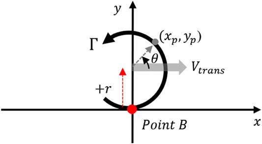
FIGURE 1. Arrangement of vortex translating past point B, illustrating the plan view of the ground plane where the tornado passes by a point situated at a distance of r from the translating path of the tornado.

The velocity components of the vortex can be obtained by taking the derivatives of $\phi$ in the x and y-direction, i.e.:

$V_x = \frac{\text{Γ}}{2\pi } \frac{-y_p}{{\left(x_p-\alpha V_{{\theta }_{max} }t\right)}^2+{\left(y_p\right)}^2}(2)$

$V_y= \frac{\text{Γ}}{2\pi } \frac{\left(x_p-V_{trans}t\right)}{{\left(x_p-\alpha V_{{\theta }_{max} }t\right)}^2+{\left(y_p\right)}^2}(3)$

where $\alpha$ is the dimensionless translating velocity (the ratio between the wind velocity and the translating velocity, $\alpha =\frac{V_{trans}}{V_{wind }}$ or $\alpha =\frac{V_{trans}}{V_{{\theta }_{max} }}$) and $V_{{\theta }_{max} }$ is the reference velocity (maximum tangential velocity), taken as 1 in what follows. Using Eqs 2, 3 in conjunction with the unsteady Bernoulli equation where the time derivative of the potential function, $\frac{\partial \phi }{\partial t}$ can be shown to be:

$\frac{\partial \phi }{\partial t} = \frac{\text{Γ}}{2\pi } \frac{y_p{V}_{trans}}{{\left(x_p-V_{trans}t\right)}^2+{\left(y_p\right)}^2}(4)$

And after some manipulation (see Supplementary Appendix SA), the overall pressure coefficient can be expressed as:

$C_P=C_{P_s}+C_{P_{adj}}(5)$

where $C_{P_s}$ is the stationary pressure coefficient ($C_{P_s}=-\frac{V_{total}^2}{V_{{\theta }_{max}}^2}$), $C_{P_{adj}}$ is the adjustment term for the pressure coefficient ($C_{P_{adj}}=\frac{2\frac{\partial \phi }{\partial t}}{V_{{\theta }_{max}}^2}$) and $V_{total}$ is the resultant velocity. After further manipulation the adjusted overall pressure coefficient can be expressed as (Supplementary Appendix SA):

$C_P=-\frac{r}{{\left(x_p-\alpha V_{{\theta }_{max} }t\right)}^2+y_p^2}\left[-2\alpha -r\right](6)$

where $r$ is the distance from vortex translation path (set as positive or negative depending on the vortex’s relative location to the x-axis). Thus, Eq. 6 represents the overall pressure coefficient as a function of vortex translating speed at any point. It should be noted that if the translating velocity is zero ($\alpha$ = 0), then Eq. 6 at the radial distance of $r_c$ will give the same static pressure as the Rankine vortex model (1882) (see Supplementary Appendix SA). As noted in Eq. 6, the overall pressure coefficient consists of two terms. The adjustment term ($C_{p_{adj}}$) includes a time derivative of the potential function, which is a function of the distance from the vortex centre and the velocity of vortex translation. Thus, $C_{p_{adj}}$ represents the effects arising from the movement of the vortex while $C_{P_s}$ represents the effects due to the presence of the vortex. As a result, the magnitude of $C_{p_{adj}}$ is dependent on the speed of the vortex translation, whereas if the vortex has no translation (stationary vortex), the overall pressure is solely the magnitude of $C_{P_s}$.

The impact of vortex translation on the pressure field at point $B$ is shown in Figure 2, where the vortex translates from $x=$ −4 to 4. The translating velocity of $\alpha =$ 0.1 and 0.3 were used for comparison and values of $r$ corresponding to +1 and −1. The black line in Figure 2 represents $C_{P_s},$ i.e., the pressure coefficient without the adjustment term induced by vortex translating motion. It is evident from Figure 2 that the contribution from $C_{p_{adj}}$ can be considerable and is a function of the relative translation speed of the vortex. For example, when $\alpha =$ 0.1 and $t=0$ (where circulation centre is at $x=0$ and $C_P$ is maximum), Eq. 6 reduces to $+/-2\alpha$. Thus, the overall value of $C_P$ increases (decreases) by 20% (−20%) depending on the value (and sign) of $r$. However, it is significant to point out that when $\alpha =$ 0.3, the changes are observed to be $\pm$ 60%. Such drastic changes in static pressure magnitude could have important implications from a design perspective.

FIGURE 2

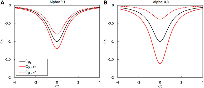
FIGURE 2. Comparison of the distribution of pressure coefficient at point B when point B is positioned at the distance of + r and - r from the vortex translating path with the translating velocity of (A) 0.1 and (B) 0.3.

Results presented in this section have shown that vortex translation is important and can have significant impact on the static pressure field. It was demonstrated that the pressure adjustment, $C_{p_{adj}}$, is dependent on the translating speed of the vortex; However, this only represents the static pressure at a particular point in space. Understandably, the superposition principle, which is valid in potential flow, could be somewhat questionable in real flows. Nevertheless, in what follows it will be shown that the potential flow framework is useful in terms of providing insight into the effects of vortex translation.

2.2 Vortex Translating Past a Body

The previous section illustrated the potentially large changes in pressure which could occur at a point due to vortex translation. In order to conduct an extensive evaluation of the impact of tornado translation on the pressure field and overall force on a body, the flow around a two-dimensional body is considered. A thin symmetrical airfoil was chosen to represent the body as the streamlined geometric configuration should minimise flow separation. Additionally, the particular airfoil cases examined are well documented, and there are reliable analytical methods which have proven to be accurate for calculating the lift force on this shape (Mittal and Saxena, 2002; Akbari and Price, 2003; Hoarau et al., 2006; Hu and Yang, 2008; Liu et al., 2012; Al Mutairi et al., 2017); such comparisons need to be made with care as implicit in our analysis is the assumption that the flow is two-dimensional which is clearly not the case for low-rise structures. However, for the purposes of the current paper this assumption is considered reasonable. The configuration of the simulation is shown in Figure 3, which illustrates the plan view of the 2D ground plane of a fixed reference frame. Similar to the configuration considered in Section 2.1, the airfoil is placed at a distance of $r$ from the translating path of the vortex with the leading edge of the airfoil positioned at the origin. The vortex rotates in the anti-clockwise direction with the circulation strength of $\text{Γ}$ and translates in the direction parallel to the x-axis from $-x$ to + $x$ with the dimensionless translating speed $\alpha$. The lift force in this context can be considered to be analogous to the side force of a 2-D body (e.g., low-rise structures) when viewed in plan; where positive lift denotes the force towards the circulation centre of the vortex while negative lift denotes the force away the circulation centre of the vortex. Given the symmetrical nature of the system, only the results relating to positive values of $r$ will be discussed in what follows as it yields greater magnitude of lift force.

FIGURE 3

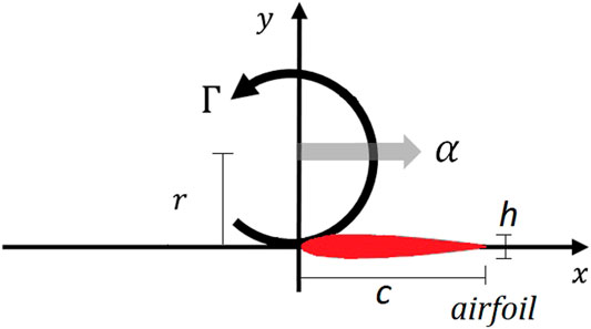
FIGURE 3. Arrangement of vortex translating past an airfoil, illustrating the plan view of the ground plane where the tornado passes by a body situated at a distance of r from the translating path of the tornado.

Several cases were devised, details of all cases explored in this study are listed in Table 1. Case 1 represents the vortex translation past a point in the flow field (as presented in Section 2.1). Case 2 investigates the impact of varying thickness of the airfoil by considering three airfoils with varying thickness, $h/c=$ 0.12, 0.24 and 0.06 corresponding to Case 2a, Case 2b and Case 2c respectively. The chord length, $c$ of the airfoil in each case is $c=$ 1 with the distance to the vortex translating path centre of $r=$ 2, resulting in a relative scale of $c/r$ = 0.5. Case 3 explores the effects of scaling where varying airfoil chord lengths and distance to the vortex translating path are simulated and compared. For this case, three different distances from the vortex translating path where examined: $r$ = 1, 2, and 4. In addition, three airfoils with varying chord lengths of $c=$ 1, 0.5, and 0.25 denoted as Case 3a, Case 3b and Case 3c respectively were simulated. This resulted in relative scales of $c/r$ = 1, 0.5 and 0.25 for Case 3a, . = 0.5, 0.25 and 0.125 for Case 3b and $c/r$ = 0.25, 0.125, and 0.0625 for Case 3c.

TABLE 1

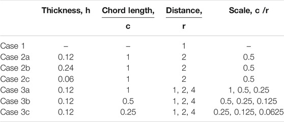
TABLE 1. Details of all simulated cases.

2.2.1 Flow Around the Airfoil

The panel method is used to compute the flow around the airfoil and obtain the lift force. The panel method is outlined fully in Hess and Smith (1967) and Rubbert (1964), but for the benefit of the reader briefly summarised below with the underlying derivations shown in Supplementary Appendix SB. The panel method considers the surface of the body to be composed of a number of discrete elements with each panel considered to be either a source or sink on which a vortex element can be placed. Each panel needs to satisfy a certain boundary condition and the linear summation of all panels is used to ultimately calculate the overall force on the body. Whilst the method is based on inviscid flow analysis and thus limited to only the resultant pressure force, the panel method has been shown to predict the aerodynamic properties of a streamlined body such as an airfoil relatively accurately (Eppler and Somers, 1979; Drela, 1989; Santana et al., 2012; Liu, 2018). The airfoil is modelled using the flow elements of source and vortex panels to represent the surface of the airfoil. In addition, the following assumptions were made for the simulation:

1. The flow is incompressible and wake effects are not considered. It is acknowledged this places limitations on the current analysis, but for the purposes of this paper the approach adopted is considered reasonable.

2. In keeping with analysis in Section 2.1, the vortex is assumed to translate with a constant velocity and does not change shape.

3. The airfoil is situated at the radius where the maximum circumferential velocity occurs and the pressure field on the surface of the airfoil is obtained by using the Bernoulli equation for unsteady flows.

Noting all of the above, the potential function of the flow field of a vortex moving past an airfoil can thus be expressed as:

$\phi = {\phi }_v+\underset{VPM}{\underbrace{{\phi }_{sourcePanel}+{\phi }_{vortexPanels}}}(7)$

where ${\phi }_v$ is the potential of the moving vortex from Eq. 1, VPM corresponds to the vortex panel method, and ${\phi }_{sourcePanel}$ and ${\phi }_{vortexPanels}$ are the source and panel terms used in the VPM. Thus, at any specific panel i, Eq. 7 can be written as:

${\phi }_i= \frac{-\text{Γ}}{2\pi }\theta +\underset{VPM}{\underbrace{{\displaystyle \sum }_{j=1}^N\frac{{\lambda }_j}{2\pi }{{\displaystyle \int }}_1^N\frac{\partial }{\partial n_i}\ln \left(r_{ij}\right)d{s}_i+{\displaystyle \sum }_{j=1}^N\frac{{\gamma }_j}{2\pi }{{\displaystyle \int }}_1^N\frac{\partial {\theta }_{ij}}{\partial n_i}d{s}_i}}(8)$

where $\text{Γ}$ is the circulation strength of the vortex, $\theta$ is the azimuth angle, $j$ is the number of the panel, $N$ is the total number of panels used to represent the body, ${\lambda }_j$ is the source strength of each individual panel, $n$ is the normal/tangential velocity component on the panel, $r_{ij}$ is the distance between the control point of the first panel, $i$ to the $j^{th}$ panel, $s_j$ is the length of each panel and ${\gamma }_j$ is the vortex strength of the panels. The panels are labelled where the first panel, $j$ = 1, begins from the bottom side of the trailing edge, in the clockwise direction and ends with panel $j$ = $N$ on the top side of the trailing edge. In order to ensure the prescribed flow element will not penetrate through the panels and the flow would be directed/deflected around the airfoil, the source and vortex strength of each individual panels are solved subject to certain boundary conditions (see Supplementary Appendix SB for further details).

2.2.2 Impact of Varying Thickness

In this section, the impact of varying thickness on the overall pressure and force on an airfoil is examined. Figure 4 shows the lift coefficient of the airfoil with the thickness of $h/c=$ 0.12 (Case 2a) due to vortex translation under the translating velocities of $\alpha =$ 0.1 and, in keeping with the analysis in Section 2.1, a higher translating velocity of $\alpha =$ 0.3 for comparison. The translating position of the vortex circulation centre is denoted as x/c with the corresponding magnitude of lift coefficient. The black lines represents $C_{L_s}$, the lift coefficient without adjustments for translation effects while the red lines represents the overall lift coefficient, $C_L$ ($C_L=C_{L_s}+C_{L_{adj}}$). It can be observed that the magnitude of the adjustments to the $C_L$ are highly similar with $C_{L_s}$, appearing to overlap each other, suggesting that the magnitude of translating velocity has a negligible effect on the overall lift. The subsequent section will further explore this further. Additionally, it can also be observed from Figure 4 that the lift on the airfoil changes with respect to the location of the vortex. The value of $C_L$ of the airfoil is relatively small when the vortex is far away ($x/c$ <-4) and then rapidly increases when the vortex approaches. The maximum value of $C_L$ is observed to occur when the vortex centre is at $x/c=-1$ (i.e., when the maximum tangential velocity is at the leading edge of the airfoil), and then rapidly decreases to a minimum $C_{L_s}$ when the vortex circulation centre is at $x/c=2$. As will be discussed later, this is due to a negative angle of attack (AoA) and thus negative lift (further details in Section 2.2.3). As the vortex translates away from the body ($x/c>4$ ), the relative inflow angle increases and $C_L$ then gradually increases. The magnitude of $C_{L_s }$ is identical for both translating velocities of $\alpha =$ 0.1 and 0.3 at approximately 2.4; this is to be expected as $C_{L_s}$ is contains no adjustment for vortex translation. Since the circulation strength of the vortex is identical for both translating velocities, the resulting $C_L$ are identical. Furthermore, the overall lift coefficient, $C_L$ shows very minimal changes as the magnitude of the translation adjustments are exceedingly low with 0.08 and 0.95% for $\alpha =$ 0.1 and 0.3 respectively. Again, the magnitude of translating velocity appears to have negligible effect on the overall lift.

FIGURE 4

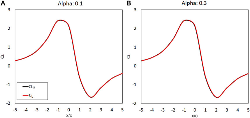
FIGURE 4. The lift coefficient of the $h/c=$ 0.12 airfoil (Case 2a) with and without translation adjustment under the translating velocities of $\alpha =$ 0.1 (A) and 0.3 (B).

Figures 5A–D shows the comparison of the magnitude of adjustments to the surface pressure distribution on the airfoil $h/c=$ 0.12 (Case 2a) and $h/c=$ 0.24 (Case 2b) at the time instance where the vortex circulation centre is at $x/c=0$. The surface distribution of overall pressure coefficient (where $C_P=C_{P_s}+C_{P_{adj}}$) of the airfoil for translation speeds of $\alpha =$ 0.1 and 0.3 are presented. The profiles in black represent $C_{P_s}$ while the profiles in red represent the overall pressure coefficient, $C_P$. It can be noticed that the overall surface pressure distribution shifts with an increase in translating velocity, $\alpha$, of the vortex where the magnitude of adjustments are considerably more distinguishable on the surface pressure coefficient than on the lift coefficient (as illustrated in Figure 4). The magnitude of adjustments, $C_{P_{adj}}$, are also observed to increase with the increase in translation velocity, from 2 to 8% in Figures 5A,B respectively, and from 3 to 10% in Figures 5C,D respectively. It should also be pointed out that the increase in thickness results in the increase in the magnitude of adjustments. This is due to the time derivative term, $\frac{\partial \phi }{\partial t}$ as presented in equation [A2], which is a function of both the distance from the vortex centre and the velocity of vortex translation. Therefore, the thicker/wider the body, the greater the adjustments, hence the greater the overall surface pressure.

FIGURE 5

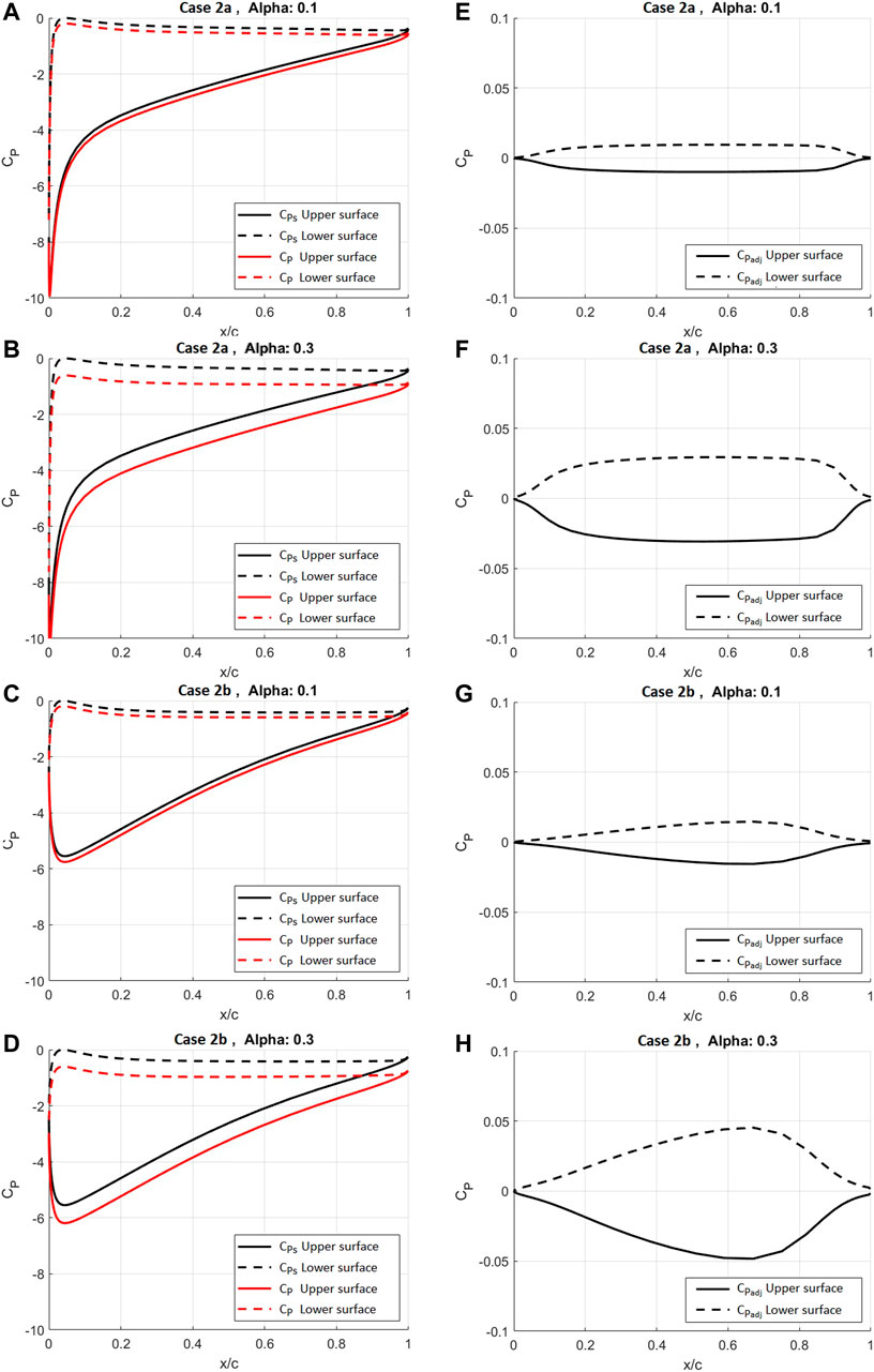
FIGURE 5. The upper and lower surface distribution of (A) pressure on the $h/c=$ 0.12 airfoil (Case 2a) with the translating velocity of 0.1, (B) 0.3, pressure on the $h/c=$ 0.24 airfoil (Case 2b) with the translating velocity of (C) 0.1 and (D) 0.3, (E) $C_{P_{adj}}$ on the $h/c=$ 0.12 airfoil (Case 2a) with the translating velocity of 0.1, (F) 0.3, (G) $C_{P_{adj}}$ on the airfoil $h/c=$ 0.24 (Case 2b) with the translating velocity of 0.1 and (H) 0.3.

Corresponding with the surface pressure as presented in Figures 5A–D; Figures 5E–H shows the $C_{P_{adj}}$ in the y-direction (lift force direction). Figures 5 E,F illustrates Case 2a where the vortex translates with the velocities of $\alpha =$ 0.1 and 0.3 respectively, while Figures 5G,H shows the thicker airfoil of Case 2b where the vortex translates with the velocities of $\alpha =$ 0.1 and 0.3 respectively. It can be observed that due to the symmetrical geometry of both of the airfoils, the pressure adjustment coefficient shows very symmetrical distribution on both the upper and lower surface of the airfoil in all cases, with the upper surface showing only slightly greater value of $C_{P_{adj}}$. As a result, the normal forces on both sides of the airfoil almost cancel each other out, leading to the very minimal effects on the overall lift coefficient, with 0.08 and 0.96% for Case 2a at $\alpha =$ 0.1 and 0.3 respectively, and 0.22 and 2.8% for Case 2b at $\alpha =$ 0.1 and 0.3 respectively.

The correlation between airfoil thickness and the magnitude of adjustments to the pressure distribution on the airfoil is examined also; three airfoils with varying thickness with the relative scale of $c/r$ = 0.5 are compared: $h/c=$ 0.12, 0.24, and 0.06 corresponding to Case 2a, 2b, and 2c, respectively. As expected, the increase in the width/thickness of the airfoil results in a slight increase in magnitude of adjustments, and thus the overall lift coefficient, $C_L$, while no effects on the trend of lift coefficient can be observed. The maximum $C_L$ of the airfoils $h/c=$ 0.12, 0.24 and 0.06 are 2.42, 2.49 and 2.35 respectively, where the adjustments are approximately 1, 2.8 and 0.3%.

In summary, it was shown that the force on the airfoil changes significantly with respect to the location of the vortex but shows minimal changes with the magnitude of $\alpha$. This is due to the changes in $C_{P_{adj}}$ on both sides of the airfoil cancelling each other out, leading to the very low changes on the overall lift coefficient. On the contrary, $C_{P_{adj}}$ increases with the increase in $\alpha$ as well as thickness/width of the body, leading to the increase in overall surface pressure. With respect to loading on low-rise structures, this suggests that overall side forces might not be affected significantly by these translation-related pressure adjustments, but surface pressure loading (such a cladding loads) might be affected. Finally, the variation of the thickness of the body does not appear to affect the lift coefficient, but only the overall magnitude of $C_L$.

2.2.3 Investigation on the Effects of Relative Scales

In this section, the effects of varying scales on the lift on an airfoil is explored and the correlation between lift coefficient and the relative inflow angle due to the translating vortex are analysed.

Figure 6 shows the comparison of lift coefficients with varying relative scales. The airfoil was positioned at three different distances from the vortex translating path of $r$ = 1, 2 and 4 with the vortex translating velocity of $\alpha =$ 0.1. The chord lengths of $c=$ 1, 0.5 and 0.25 (Case 3a, Case 3b, and Case 3c respectively) are shown in Figures 6A–C respectively, yielding with the relative scale of $c/r$ = 1, 0.5 and 0.25 for Case 3a, $c/r$ = 0.5, 0.25 and 0.125 for Case 3b and $c/r$ = 0.25, 0.125 and 0.0625 for Case 3c. The translating position of the vortex circulation centre is denoted with $x/c$ with the corresponding magnitude of lift coefficient.

FIGURE 6

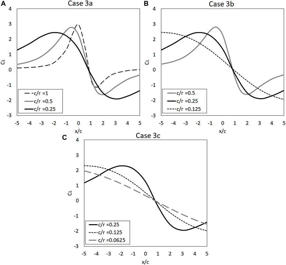
FIGURE 6. The lift coefficient of the airfoil with the chord lengths of c= 1, 0.5 and 0.25 corresponding to (A) Case 3a, (B) Case 3b and (C) Case 3c, respectively.

Generally, it can be observed that the lift coefficient is primarily affected by the relative scale of the airfoil to the vortex and the location of the vortex circulation centre. When the airfoil is situated closest to the vortex translating path (i.e., the scale of $c/r$ = 1 in Figure 6A), the variation in $C_{L_s}$ appears to be more concentrated but spreads out when the distance from the vortex translating path increases. For the scale of $c/r$ = 1, the lift coefficient is highly affected by the location of the vortex, i.e., the induced vortex effects appear to occur over a relatively a shorter range of x-distances. However, for the case with particularly high difference in relative scale of $c/r$ = 0.0625, Figure 6C shows the $C_{L_s}$ variation is almost linear. Additionally, Figure 6 clearly shows that the distribution of lift is dependent on the location of the vortex. As the vortex translates away from the airfoil, $x/c$ >1, the relative AoA for all scales are negative resulting in negative values of $C_L$. Furthermore, the maximum lift coefficient is observed to decreases with the decrease in relative scale. Details of the magnitude of maximum lift coefficient ($C_L$) are listed in Table 2.

TABLE 2

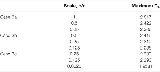
TABLE 2. Details of the maximum magnitude of lift coefficient for all Case 3a, 3b, and 3c.

Overall, it was found that the effects of varying relative scales of the airfoil to the vortex is crucial and significantly changes the lift coefficient, where the primary factor affecting the lift on the airfoil is due to the relative inflow angle, which is attributed to the location of the vortex. As the vortex flow is circular, the increase in the size of the airfoil and distance from the vortex translating path will likely alter the inflow angle of the vortex. Therefore, the difference between the inflow angle at the leading and trailing edge for the varying scales are further explored.

Figure 7 shows the relative inflow angle at the leading edge ($x/c$ = 0) and the outflow angle at the trailing edge ($x/c$ = 1) of the airfoil for three different sizes of airfoils (Case 3a, Case 3b and Case 3c). The translating position of the vortex circulation centre is denoted with $x/c$ with the corresponding flow angles, AoA. As shown in Figure 7, for cases where the airfoil is close to the vortex translating path, $r$ = 1, it can be observed that when the vortex circulation centre is very far away ($x/c$ <-4), the inflow and outflow angles are approximately 80^o. The flow angle gradually decreases as the vortex approaches the airfoil. At $x/c$ = 0, the inflow angle at the leading edge is 0^o as the flow is tangential to the airfoil while the outflow angle at the trailing edge is 45^o, 26.6^o and 14^o for the scales $c/r$ = 1, 0.5 and 0.25 respectively. As the vortex translates past the airfoil, the flow angles continue to decrease and approach −80^o when the vortex circulation centre is very far away ($x/c$ >4).

FIGURE 7

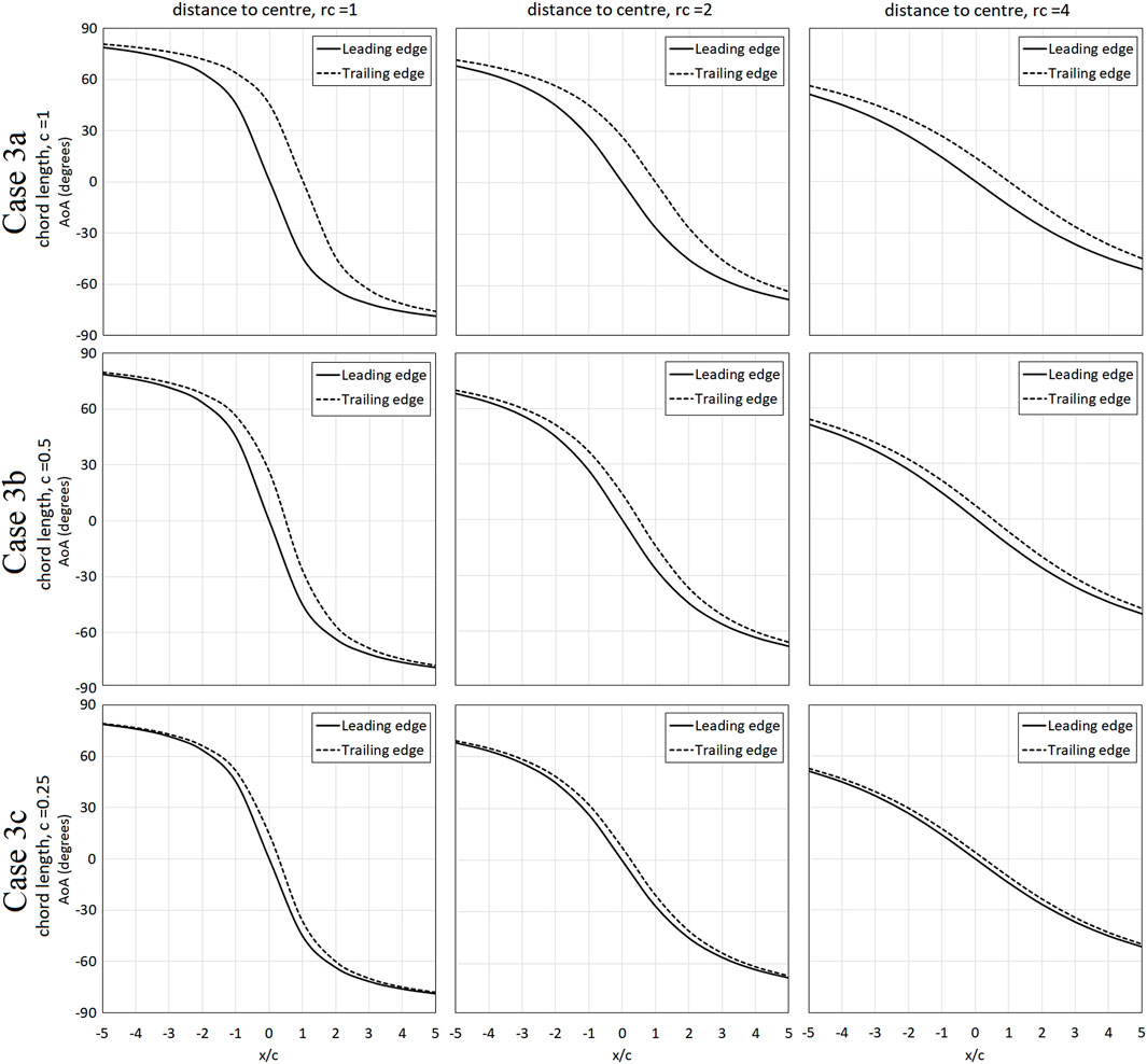
FIGURE 7. The inflow angle at the leading edge ($x/c$ = 0) and the outflow angle at the trailing edge ($x/c$ = 1) for three different sizes of airfoils (Case 3a, Case 3b and Case 3c). Note that the difference in flow angle between the leading and trailing edges decreases with both smaller airfoil size (moving down on the page) and with greater distance between the airfoil and the vortex (moving to the right).

It should be pointed out that the difference between inflow and outflow angles when the vortex is directly above the airfoil at $x/c$ = 0 for cases with the same scales are identical (e.g. when the vortex circulation centre is at $x$ = 0, the difference between inflow and outflow angles are 28.4 for both Case 3a with $c$ = 1, $r$ = 2 and Case 3b with $c$ = 0.5 and $r$ = 1); however, during the approaching of the vortex ($x/c$ <0) and leaving of the vortex ($x/c$ >0), the difference between inflow and outflow angles are slightly different. It is postulated that the combination of similar inflow angle difference and the specific flow angle induced by the vortex resulted in the similar a trend of lift coefficient of the airfoil with the same scale. Overall, a general trend can be observed for all 3 cases where the increase in distance from $r$ = 1 to 4 results in the smoothening of the flow angles at both the leading and trailing edge, while the decrease in the length of the chord from $c$ = 1 to 0.25 results in the decrease in difference between the flow angles at both the leading and trailing edge.

Figure 8 illustrates the lift coefficient of the airfoil due to translating vortex with varying relative scales (as presented in Figure 6) in comparison with the lift coefficient of an airfoil in uniform flow with the angles of attack corresponding to the inflow angles as presented in Figure 7. The red solid line represents the lift coefficients of the airfoil due to vortex translation, denoted with “vortex flow” while the black solid line represents the lift coefficient of an airfoil in uniform flow subjected to the AoA based on the inflow angle at the leading edge, denoted with “uniform flow, leading edge” and the black dotted line represents the lift coefficient of an airfoil in uniform subjected to the AoA based on the outflow angle at the trailing edge, denoted with “uniform flow, trailing edge” as presented in Figure 7; thus, depicting the lift changes of an airfoil in uniform flow subjected to identical inflow and outflow angle instead of circular flows. Generally, for all scales of Case 3a, it can be observed that while the lift coefficients of the airfoil in vortex flow (vortex flow) for all three scales, $c/r$ = 1, 0.5 and 0.25 does not correspond with the airfoil in uniform flows, when the vortex circulation centre is far away, the trend of lift coefficient falls well within the range between the lift coefficient of the uniform flow approximations when the vortex circulation centre is close to the airfoil at $x/c=-$ 1 to 2. For three scales of case 3b, the lift coefficients for uniform flows and vortex flows does not correspond well but shows a similar general trend. This can also be observed for the scales of $c/r$ = 0.125 and 0.0625 of case 3c, while the lift coefficient of the scale $c/r$ = 0.25 matches the lift coefficient of the uniform flow approximations when the vortex is far away at $x/c<-$ 3 and 3.

FIGURE 8

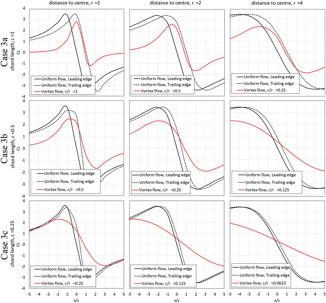
FIGURE 8. The comparison of the lift coefficient of the airfoil due to translating vortex with varying relative scales and vortex in uniform flows.

Generally, the magnitude of maximum $C_L$ (of airfoil in vortex flows) is marginally greater than the minimum $C_L$ for all scales, resulting with the lift coefficient that is somewhat symmetrical about the $x/c$ = 0 axis. However, the scale $c/r$ = 1 for Case 3a (as shown in Figure 8) this difference is particularly noticeable, where the lift coefficient is highly asymmetrical about $x/c=0$ despite the symmetrical inflow angle at the leading edge when the x-position of the vortex centre is $x/c$ <0 and the inflow angle when the x-position of the vortex centre is $x/c$ >0. This is due to the contribution of vortex pressure. Since this is a potential flow simulation and the simulated vortex is a free vortex, the velocity increases with the increase towards the centre of the circulation, resulting in high magnitude of velocity, thus decreasing the pressure on the upper surface of the airfoil and greatly increasing the lift, particularly when the vortex is above the airfoil, when the vortex circulation centre is at $x/c$ = 0 as demonstrated in Figure 8. With the vortex translating away from the airfoil, the absence of vortex pressure on lift resulted in the low magnitude of lift despite the identical inflow angle (albeit with a negative sign). It should also be pointed out that the stall angle for a symmetrical airfoil generally occurs between 15^o and 20^o (as reported by Michos et al., 1983), thus, the high relative inflow angle as presented in this section is undoubtably unrealistic and would result in the stalling of the airfoil. However, this does not impact the implicit point being made, i.e., that a translating vortex affects streamline curvature resulting in changes of angle of attack, and these AoA can result in a very different flow field over large parts of the body than what can be simulated with a uniform flow.

Figure 9 presents the maximum difference in flow angles between the leading edge and the trailing edge corresponding to all scales for Case 3a, 3b and 3c as shown in Figure 7, hence, highlighting the range of relative inflow angles induced by vortex translation on the airfoil with varying chord lengths and distance to the vortex translating path. It can be observed that the difference in flow angles for the same scale are highly similar (i.e., the difference in flow angles for the scale $c/r$ = 0.5 with $c$ = 1 and $r$ = 2 for case 3a and the scale $c/r$ = 0.5 with $c$ = 0.5 and $r$ = 1 for case 3b are both 26°). This is due to the identical ratio between the length of the airfoil and the distance from the vortex translating path, thus, the difference between the inflow angle at the leading and trailing edge is similar as the flow is approximately circular. As a result, all three cases shows a very similar trend of range of inflow angles, where the range of angles decreases with the decrease in scale.

FIGURE 9

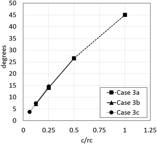
FIGURE 9. The maximum difference in flow angles between the leading edge and the trailing edge corresponding to all scales for Case 3a, 3b, and 3c.

Overall, exploring the effects of varying scales on the lift of an airfoil found that the primary factor affecting the lift changes is the relative inflow angle which is dependent on the location of the vortex. The lift coefficients are shown to spread out with the decrease in relative scale, while the maximum $C_L$ decreases with the decrease in relative scale. Examination of the flow angles revealed that the increase in distance from the vortex centre results in the flattening of the trend of flow angles at both the leading and trailing edge, whilst the decrease in the length of the chord decreases the differences between the flow angles at both the leading and trailing edge. In other words, since the flow is approximately circular, the difference between the inflow angle at the leading and trailing edge can be expressed as a ratio between the chord length and distance to the vortex translating path.

Additionally, by considering the flow angles at both the leading edge and the trailing edge, it was shown that the trend of lift coefficient of the airfoil in vortex flow falls within the range of the lift coefficient of airfoil in uniform flows with the corresponding AoA. Whilst noticeable differences can be observed between results from these simulations (airfoil in vortex flows and uniform flows), this is to be expected as these flows are fundamentally different. The lift of the airfoil in a vortex flow results from varying inflow angles due to streamline curvature that is dependent on the location of the vortex circulation centre and the relative scale of the airfoil. Therefore, the idea that the maximum forces on a body subjected to a moving tornado/vortex can be predicted using uniform flow without simulating a moving vortex, provided that the appropriate range of inflow angles are known will be further discussed in Section 4.

3. Tornado Translating Velocity

The previous sections illustrated the substantial increase in pressure which occurs at a point and on the surface of the airfoil due to vortex translation. While the translating speed of the vortex, $\alpha$, only has minimal affects on the overall lift on the airfoil, the pressure adjustment, $C_{P_{adj}}$ on the surface of the airfoil was shown to be dependent on the magnitude of the translating speed of the vortex and increases with the increase in $\alpha$. Thus, it is significant to assess actual ranges of translation speeds of naturally occurring tornadoes in order to determine the possible practical importance of these of potential flow results.

The Storm Events database of NOAA (NOAA, 2012) is used for the analysis. At the time of analysis, the database contained records of tornadoes occurring between 1950 and 2020. These records tend to be classified using either the F scale or the EF scale. Due to the absence of the recorded (tangential) wind speed of some tornadoes, it is not possible to convert all of the tornadoes to a single scale, e.g., the EF scale. Hence, in what follows, results are initially analysed separately for each category. It should also be noted that not all of the data in the database contains complete information regarding the start and end location of the tornado occurrence as well as the duration of the occurrence. This, where this is the case, the data for this event is considered to be incomplete and excluded from the calculation. This is particularly true for data between 1950 and 1992 which accounts for a large portion of the incomplete data (details in Section 3.1). Finally, we have also taken the unusual step of analysing the results in dimensional and nondimensional form for reasons that will become self-evident below.

3.1 Analysis

The number of tornado occurrences based on the F scale (from 1950 to 2007) and EF scale (from 2007 to 2020) are shown in Figures 10A,B. Attributed to each section of Figures 10A,B are two different percentage values: the first percentage indicates the total number of records in each dataset corresponding to that scale, whilst the second percentage (the figure in brackets) corresponds to the amount of data at a particular scale which is complete and hence used in the analysis. For example, in Figure 10A, F1 scale data accounts for 34% of all of the F scale tornadoes in the data set but only 12% of these are complete and used in the analysis. In total, 4,830 and 16,967 tornadoes corresponding to F scale and EF scale tornadoes respectively have been considered below. Figure 10 indicates that in general, F0 and EF0 scale activity accounts for majority of the tornado occurrences (39 and 52% respectively), while tornado occurrences corresponding to the either F4/5 or EF4/5 are considerably less frequent (2% or less in both cases).

FIGURE 10

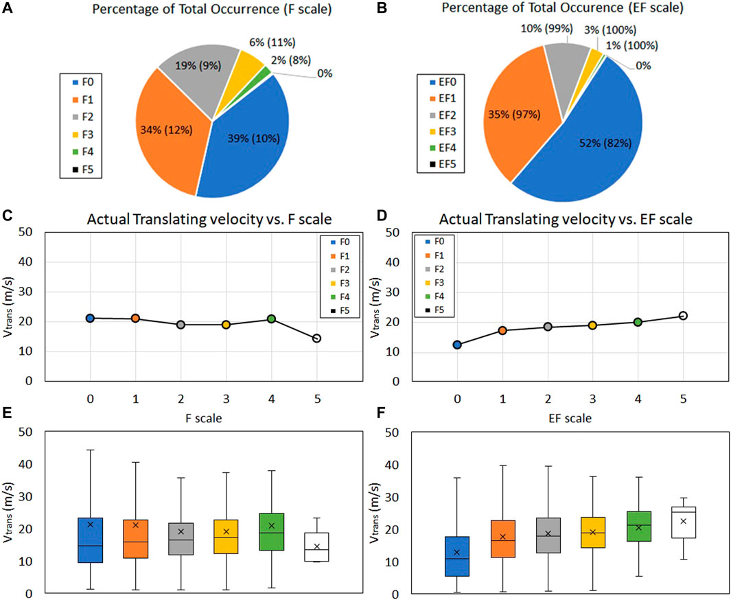
FIGURE 10. The number of tornado occurrence based on (A) F scales from 1950 to 2007 (B) EF scales from 2007 to 2020. Translating velocity of tornadoes according to the (C) F scale (D) EF scale. The box and whisker plot of the distribution of data corresponding to (E) F scale (F) EF scale.

The mean translating velocity ($V_{trans}$) of each tornado is based on the simple calculation of translated distance/duration. Translated distance in this context is calculated using the start and end longitudes and latitudes and assumes a straight-line translation. Thus, the calculated distance travelled is rather arbitrary but for the purposes of the current analysis is considered suitable. The duration parameter is simply obtained from the difference between the end time of the tornado and the start time–both data are given in the database. Similar to the distance calculation, this may not be wholly accurate but, for the purposes of the current analysis, it has been assumed that the data in the database is sufficiently accurate. Figures 10C,D illustrates the calculated translating velocity against scale and suggest that, on average, there is relatively little variation in the translating velocity regardless of scale, i.e., average values ∼19 m/s (see Table 3). However, as indicated in Figures 10E,F significant variations exist within each scale with the possible exception of F/EF 5 data, which is likely due to an artifact from the lack of data (at high return periods); further, the trend as shown in Figures 10A,B suggests that this could simply be due to there being insufficient records in these categories making the drawing of meaningful conclusions rather difficult. Thus, while the actual translating speed appears to be independent of the scale of the tornado, it should be interpreted with care.

TABLE 3

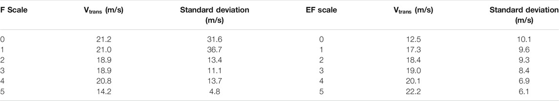
TABLE 3. Details of the mean translating velocity and standard deviation of recorded tornado data based on F and EF scales.

Understandably, with the improvement of tornado reporting and measurement, the more recent data (EF scale data) are significantly more comprehensive and contains less missing information. Thus, further analysis are conducted only using the EF scales. The typical ranges of wind speed that each EF scale covers were used to convert EF scales to actual wind speeds. For each scale, a simple average velocity ($V_{wind }$) has been obtained using the maximum and minimum values of the range; however, for EF5, $V_{wind }$ is simply taken to be equivalent to the lowest 3 s gust velocity. Thus, for EF scales of 0, 1, 2, 3, 4, and 5, the average wind velocities are 33.5 m/s, 43.8 m/s, 54.9 m/s, 67.3 m/s 81.8 m/s, and 89.4 m/s respectively. Whilst this is highly inconsistent, it has already been noted above that the data in these categories are too sparse to enable any meaningful conclusions to be drawn. The normalising of the data in this way introduces an additional unknown, namely the difference between the mean values in a particular range and the two extremes of that range, where the uncertainties for the EF scales of 0, 1, 2, 3, 4, and 5 are 13, 12, 10, 10 and 9% respectively. Given the variability within each scale as shown in Figure 10, what follows should be interpreted with caution.

Figure 11A shows the normalised translating velocity, $\alpha$ (where $=V_{trans} /V_{wind }$) of tornadoes of EF scale whilst Figure 11B illustrates the variation in the data. The translating velocity, $\alpha$ for EF scale 0, 1, 2, 3, 4, and 5 are 0.37, 0.39, 0.34, 0.28, 0.25, and 0.25 respectively, while the standard deviation for the corresponding EF scales are 0.3, 0.22, 0.17, 0.13 0.08, and 0.07 respectively. Figure 11A indicates a minor decrease in $\alpha$ as the scale increases, i.e., in relative terms the translation speed varies slightly with respect to tornado scale. However, this is expected as the average wind velocity increases with the increase in scale.

FIGURE 11

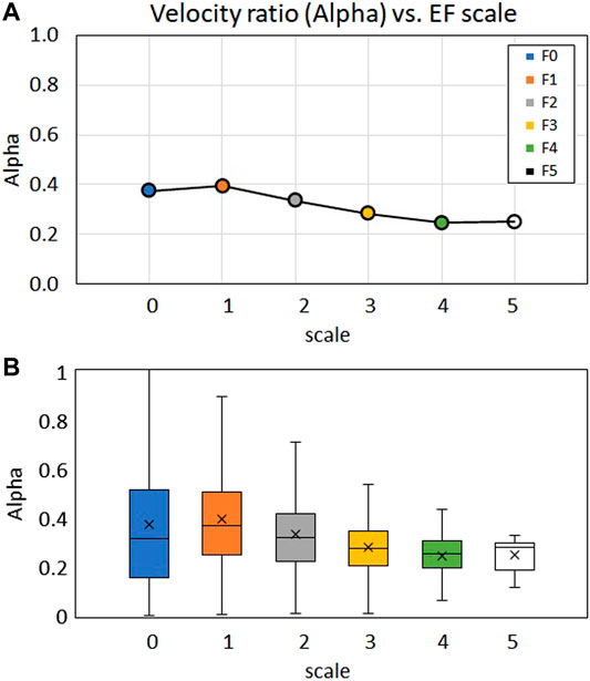
FIGURE 11. (A) Normalised translating velocity of tornadoes of EF scale. (B) The box and whisker plot of the distribution of data.

Notwithstanding the additional variability that has been introduced by non-dimenisonalising the data, with the similarity in the mean translating velocities (both the F and EF scales as presented in Figure 10), it is evident that the translating velocities of tornadoes are independent of scales, thus permitting all data to be combined. As a result, all data of the EF scale are combined (denoted as “combined scale”) and further analysed. Additionally, due to the lack of sufficient data for the scales with higher uncertainties (EF0, EF1, and EF 5) these data have been removed for the purpose of this analysis.

The mean translating velocity of the combined scale data is 18.8 m/s with the standard deviation of 10.57 m/s and the skewness and Kurtosis of 3.45 and 24.26 respectively, while the normalised mean translating velocity is 0.32 with the standard deviation of 0.17 and the skewness and Kurtosis of 2.68 and 19.48 respectively. In comparison, the dimensional results have marginally higher skewness as well as kurtosis in comparison with the normalised data. This difference can be attributed to the normalising process as tornadoes at each scales were normalised with the respective mean wind velocity, thus resulting in the difference in skewness and kurtosis. Additionally, an analysis was conducted using the 3-parameter Weibull probability density function. It was found that by using the shape parameter, $\beta$ of 3, scale parameter, $\eta$ of 31, and location parameter $\gamma$ of 10, the Weibull probability density function fits the combined scaled data very well.

Overall, results presented in this section demonstrated that while the average wind velocity of tornadoes varies drastically depending on the magnitude of the respective scales (F and EF scale), the actual translating speed of tornadoes are independent of the scales. The mean translating velocity of tornadoes is 18.8 m/s with a normalised mean translating velocity of 0.32, but with the possibility of translating up to the normalised velocity of 0.37. Having established the relative range of translating speeds which occur in naturally occurring tornadoes, it is now possible to explore the effect that such a range may have on the generated pressure field and force coefficient.

4 Application of Methodology

In this section, the framework to reproduce the flow conditions and effects of a moving tornado is proposed. The correlation between flow angles and the relative scale of the airfoil to the vortex is discussed and the expression summarising the adjustments required to account for the pressure increase due to vortex translation is explored. Finally, the procedure of application using the proposed methodology is presented.

4.1 Range of Flow Angles

Results presented in Section 2.2.3 have shown that by considering the flow angles at both the leading edge and the trailing edge, the maximum forces on an airfoil subjected to a moving vortex can be predicted using uniform flow with the appropriate range of inflow angles. However (as presented in Section 2.2.3), varying the chord lengths and distances from the vortex translating path will result in a range of flow angles; thus, an expression summarising the flow angle and the relative scale of the airfoil to the vortex is presented below.

Based on Figure 9, it can be observed that all three cases show similar trends, where the range of angles decreases with the decrease in scale. Thus, it is possible to fit a curve to obtain an expression containing the chord length and distance from the vortex translating path:

$\text{Θ}= -15.7 {(c/r)}^2 +61.03(c/r)-0.05(9)$

where $\text{Θ}$ is the maximum difference in inflow angle between the leading edge and the trailing edge. It should be acknowledged that Eq. 9 does not contain any variable regarding the AoA in order to obtain the maximum lift on an airfoil. As noted above, the current analysis does not consider flow separation and as such Eq. 9 should be considered as conservative.

4.2 Adjustments for Surface Pressure

Initially, Case 1 which represents vortex translation past a point with no body present in the flow is explored. The maximum adjustments to the pressure coefficient, $C_{p_{adj}}$ at the point $x$ = 0 and $y=r$ with the vortex translating velocities of $\alpha =$ 0.1, 0.2, 0.3, 0.4 and 0.5 are shown in Figure 12A. Based on this figure, it can be observed that $C_{p_{adj}}$ increases linearly with the increase in translating velocity with a gradient of 2. Thus, in the overall pressure coefficient Eq. 5, the adjustment term, $C_{p_{adj}}$ is replaced with $\alpha$, as a function of vortex translating velocity, as:

$C_P= C_{P_s}+2\alpha (10)$

where $C_{P_s}$ can be obtained using equation [A7]. The resulting expression as presented in Eq. 10 can be used to estimate the maximum overall pressure coefficient at point under varying vortex translating velocities. Next, in order to quantify the impact of vortex translation on the surface pressure coefficient on the airfoil, the mean value of $C_{P_{adj}}$ over the surface for all cases of Case 2 (Case 2a, 2b, and 2c) and Case 3a is calculated. It should be noted that to retain consistency, Case 3a is employed as the chord lengths are identical. Figure 12B shows the mean adjustments to the pressure coefficient on the airfoil when the vortex circulation centre is located where the maximum lift coefficient for the airfoil occurs, with varying airfoil thickness (Case 2) and varying relative scale (Case 3a). Figure 12B outlines the mean $C_{P_{adj}}$ of airfoil with varying thickness of $h/c=$ 0.06, 0.12 and 0.24 with the vortex circulation centre at $x/c=$ −1 and translating velocities of $\alpha =$ 0.1, 0.2, 0.3, 0.4, and 0.5. Figure 12C shows the mean $C_{P_{adj}}$ of airfoil with varying relative scales of $c/r$ = 1, 0.5 and 0.25 with the vortex circulation centre at $x/c=$−2.2, −1, and 0 respectively (as shown in Figure 6A) and translating velocities of $\alpha =$ 0.1, 0.2, 0.3, 0.4, and 0.5.

FIGURE 12

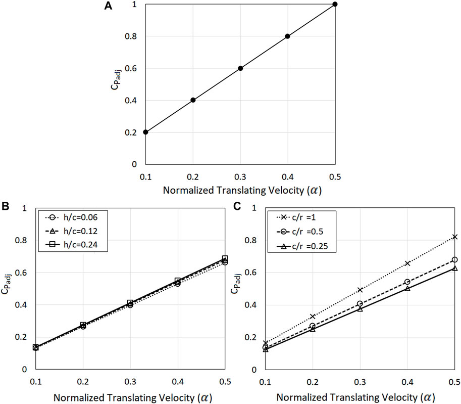
FIGURE 12. The adjustments to pressure coefficient as a function of translating velocity for (A) at the point, Case 1, where $x$ = 0 and $y=r$ when the vortex circulation centre is at $x/c$ = 0, (B) on the airfoil during maximum lift coefficient for Case 2 and (C) on the airfoil during maximum lift coefficient for Case 3a.

As illustrated in Figure 12B, whilst increasing the thickness of the airfoil results in the increase in $C_{P_{adj}}$, the translating velocity is the primary factor affecting $C_{P_{adj}}$. All three cases show linear increase with $\alpha$, with gradients of 1.32, 1.36, and 1.38 for $h/c=$ 0.06, 0.12, and 0.24, respectively. Similarly, the adjustment term, $C_{p_{adj}}$ is replaced with $\alpha$, and thus, the overall pressure coefficient can be rearranged as a function of airfoil thickness and vortex translating velocity as:

$C_P= C_{P_s}+(0.244 h/c +1.32)\alpha (11)$

Equation 11 illustrates that the overall pressure coefficient at a point is a function of translation speed and relative scale. This is an important finding since it suggests that adding the translation speed of a tornado to the maximum wind speed generated by the flow field will not result in an appropriate value for the pressure coefficient. Eq. 11 can be used to estimate the maximum overall pressure coefficient at point under varying vortex translating velocities. Additionally, the comparison of varying scales showed that the increase in relative airfoil size results in a considerable increase in $C_{P_{adj}}$; however, the major factor in the increase in adjustments can be attributed to the translating velocity of the vortex. All three scales show a linear increase with the $\alpha$, with gradients of 1.64, 1.36, and 1.25 for the scales $c/r$ = 1, 0.5 and 0.25, respectively. The overall pressure coefficient can be rearranged as a function of the relative airfoil scale to the vortex translating path and vortex translating velocity as:

$C_P= C_{P_s}+(0.526 c/r +1.1)\alpha (12)$

By combining Eqs 11, 12, it is possible to obtain a multi-parameter expression containing both the scale and airfoil thickness summarising the adjustment on an airfoil as:

$C_P= C_{P_s}+(0.244 h/c+ 0.489 c/r +1.114)\alpha (13)$

Equation 13 can be used to estimate the maximum overall pressure coefficient on the airfoil under varying vortex translating velocities, where the distribution of $C_{P_s}$ on the surface of the airfoil when the maximum lift coefficient occurs can be obtained using the range of AoA of $\text{Θ}$ as discussed in Section 4.1. With that being said, these generalised equations are unable to summarise every geometrical configuration and is limited to only the symmetrical airfoil. This may be unrealistic for bluff bodies for the reasons outlined above. Moreover, by neglecting the wake effects, additional forces induced by drag are ignored; as demonstrated in Section 2.2.3, the high relative inflow angle as experienced by the airfoil far exceeds the critical angle of attack, which is undoubtably unrealistic and would result in the stalling of the airfoil. Therefore, further physical or numerical simulations should be conducted in order to validate these generalised equations; physical vortex generators with the capability to effectively model the translation of tornadoes, although restricted to lower translating speeds (approximately 0.5–2 m/s) (Razavi and Sarkar, 2018; Refan and Hangan, 2018) could validate the effects of tornado translation on pressure on the airfoil at lower translating speeds; concurrently, CFD simulations could also provide as an alternative via using sliding mesh to simulate the translating movement, thus simulating vortex translation at higher speeds. Notwithstanding the limitations, the findings presented in this study demonstrate the significant importance of considering vortex translation on the overall pressure coefficient.

4.3 Application Procedure

Procedures to apply the proposed flow angles and pressure adjustments in Sections 4.1, 4.2 can be used in a number of ways:

• As a framework to reproduce the flow conditions of a moving tornado in which physical or numerical methods could be based upon–the force exerted on a (Civil Engineering) structure, and thus, wind load can be estimated using a typical boundary layer wind tunnel with the suggested range of flow angles, without the need to employ a vortex generator.

• To assist in determining the pressure acting on cladding of a low-rise structure in a tornadic wind field where large increase in pressure could occur, potentially lead to failure.

Identifying the relative size of the airfoil is, of course, the first step in calculating the flow angles, which includes the specification of the reference length (chord length) of the airfoil, $c$, and the distance to the tornado translating path, $r$. By using the relative scale of the airfoil to the vortex, $c/r$ , a range of angle, $\text{Θ}$, representing the maximum difference in flow angle between the leading and trailing edge can be obtained using Eq. 9 (e.g., an airfoil with the chord length of $c$ = 1 and the distance to the vortex translating path of $r$ = 2, yielding with the relative scale of $c/r$ = 0.25, the maximum difference in flow angle is approximately 14.2^o).

By employing a numerical or physical boundary layer wind tunnel, the angle of attack at which the maximum lift occurs can be obtained. The lift force in this context can be considered to be equivalent to the side force of traditional (Civil Engineering) structure when viewed in plan. It would be advisable also to simulate the additional range of +/-$\text{Θ}$; for example, for a symmetrical airfoil at Reynolds number of 179,000, the maximum $C_{L_s}$ of approximately 1.6 occurs at the AoA of approximately 10^o (Drela, 1989). Using the relative scale of $c/r$ = 0.25, the additional AoA of −4.2^o and 24.2^o with the $C_{L_s}$ of approximately −0.5 and 0.9 respectively, should also be considered. Whilst the magnitude of $C_{L_s}$ simulated at the additional AoA are (expectedly) lower than the maximum $C_{L_s}$ of 1.6, the corresponding drag coefficient, $C_D$ changes drastically, with the magnitude of approximately 0.007, 0.013 and >0.03 for −4.2^o, 10^o and 24.2^o respectively. Thus, highlighting the associated increase and decrease in force (lift or drag) that should be considered to fully account for the flow conditions as induced by a moving tornado. It is acknowledged that due to the limitations of the current methodology, the wake effects are neglected. However, this simple example demonstrates the significance of considering the effects induced by the additional angles of $\text{Θ}$. Additionally, for the calculation of force coefficient on the airfoil, the effects caused by the translating velocity is not considered as $\alpha$ was found to have very minimal effects on the overall force (as discussed in Section 2.2.2).

By conducting the simulation using physical/numerical boundary layer wind tunnel, the surface pressure distribution on the airfoil can be measured, which can be used as input to the variable of $C_{P_s}$ in Eq. 13 as well as the specification of the airfoil thickness, $h$. The increase in surface pressure distribution was observed to increase considerably with the increase in translating velocity, $\alpha$. As discussed in Section 3, it is evident that the translating velocity of tornadoes appears to be independent of the F and EF scales, with the average $\alpha$ of 0.32. Thus, using these input parameters, an airfoil with the relative scale of $c/r$ = 0.25 and thickness of $h/c=$ 0.12 will yield the adjustment of $C_{P_{adj}}=$ 0.4 to be added to every measured pressure point in order to account for the effects induced by the tornado translating movement, but can increase up to $C_{P_{adj}}=$ 0.52 with the translating velocity of $\alpha$ = 0.37. The resulting overall surface pressure distribution on the surface can be used as a reference to determine where large increase in pressure could occur, which may lead to the failure of cladding (or roof tiles) and require structural reinforcement.

Admittedly, this procedure of application as described, is a simplified approach; whilst the superposition principle is valid in potential flow, in real flow this could be somewhat questionable. Additionally, the flow is also assumed to be 2-D which is clearly not the case for a naturally occurring tornado or a physically simulated vortex; physical and numerical studies (Natarajan and Hangan, 2012; Gillmeier et al., 2017; Refan and Hangan, 2018) have shown that while the dominant flow component of tornado-like vortices is the tangential velocity, the vertical and radial velocity component could be up to the magnitude of approximately 35 and 58% of the tangential velocity respectively, therefore, the inclusion of the vertical and radial component of velocity could potentially affect the inflow angle drastically. With that being said, the findings presented in this study have shown that the framework is useful in terms of providing insight into the effects of vortex translation on the pressure field and the force on a body and providing a foundation upon which future simulation methods could be based.

5. Summary and Conclusion

In this paper, the impact of tornado translation on the pressure and overall force on a body is explored and a framework to reproduce the flow conditions and effects of a moving tornado is presented. A symmetrical airfoil was chosen to represent the body since it minimises flow separation and has an exact solution via potential flow analysis. Lift and drag on such an airfoil would be analogous to the side force on a 2D body such as a low-rise structure when viewed in plan. The model describing the vortex movement was developed using unsteady potential flow theory and the ranges of translation speeds of naturally occurring tornadoes were assessed, which were then summarised as expressions describing the characteristics of moving tornadoes. The main conclusions of the analysis are:

• Analysis of the NOAA database revealed that the average tornado translating velocity is 18.8 m/s, which is independent of the intensity of the tornado as indicated by the F and EF Scales. Considering the wind speeds in the EF scale this implies non-dimensional wind speed ratios of the translation to total wind speed ($\alpha$) in the range from 0.25 up to 0.37.

• Vortex translation has significant importance on the pressure field. The analysis on the impact of tornado translation on the pressure at a point (Case 1) showed that the magnitude of the static pressure drop increases with an increase in vortex translating velocity. The magnitude increases by 20% when the translating velocity is 10% of the tornado wind velocity but increases up to 60% when the translating velocity increases to 30% of the tangential velocity. This is due to the pressure adjustment term, $C_{p_{adj}}$, which represents the effects arising from the movement of the tornado vortex and is dependent on the magnitude of translating velocity.

• Varying the thickness of an airfoil subjected to a translating vortex (Case 2) showed that the lift changes drastically (up to a factor of 2) with respect to the relative location of the vortex but shows less than 1% increase with respect to the translating velocity (from $\alpha$ = 0.1–0.3). Lift in this case should be considered analogous to the overall side force on a structure viewed in plan. In contrast, the magnitude of pressure on the surface of the body was observed to increase approximately 10% with an increase in translating velocity as well as with an increase of thickness of the airfoil. While this surface pressure effect occurs on both sides of the airfoil and therefore does not significantly affect overall side force (as mentioned above), this pressure change is analogous to cladding loads on the surface of a structure and potentially warrants further study.

• Varying airfoil sizes and distance to the vortex translation path (Case 3) showed that the relative inflow and outflow angles induced by the vortex movement are the primary factors affecting the lift variation on the airfoil. Use of these inflow and outflow angles with uniform flow past an airfoil suggested that the maximum forces on a body subjected to a translating tornado could be predicted provided that the appropriate range of inflow and outflow angles are known.

• A framework to reproduce the flow conditions of a translating tornado using uniform flow is proposed. The expression summarising the appropriate range of flow angles based on the airfoil size and distance to the vortex translation path is outlined and the expression to estimate the maximum pressure coefficient on the airfoil under varying translation velocities are presented, which potentially exemplifies how a boundary layer wind tunnel could be used to obtain results comparable to those generated by a translating vortex simulator.

The findings presented in this paper have demonstrated the importance of tornado translation on the pressure and overall force on an airfoil and the framework was shown to be potentially useful for providing insights on the effects of vortex translation that could guide future simulation methods. However, these generalised equations are limited to the assumptions made in this study, thus should be interpreted with caution.

Data Availability Statement

The raw data supporting the conclusions of this article will be made available by the authors, without undue reservation.

Author Contributions

All authors listed have made a substantial, direct, and intellectual contribution to the work and approved it for the publication.

Conflict of Interest

The authors declare that the research was conducted in the absence of any commercial or financial relationships that could be construed as a potential conflict of interest.

Publisher’s Note

All claims expressed in this article are solely those of the authors and do not necessarily represent those of their affiliated organizations, or those of the publisher, the editors and the reviewers. Any product that may be evaluated in this article, or claim that may be made by its manufacturer, is not guaranteed or endorsed by the publisher.

Supplementary Material

The Supplementary Material for this article can be found online at: https://www.frontiersin.org/articles/10.3389/fbuil.2022.840812/full#supplementary-material

References

Akbari, M. H., and Price, S. J. (2003). Simulation of Dynamic Stall for a NACA 0012 Airfoil Using a Vortex Method. J. Fluids Structures 17, 855–874. doi:10.1016/s0889-9746(03)00018-5

CrossRef Full Text | Google Scholar

Al Mutairi, J., ElJack, E., and AlQadi, I. (2017). Dynamics of Laminar Separation Bubble over NACA-0012 Airfoil Near Stall Conditions. Aerospace Sci. Tech. 68, 193–203. 1270-9638. doi:10.1016/j.ast.2017.05.015

CrossRef Full Text | Google Scholar

Anderson, J. (2016). Fundamentals of Aerodynamics. 6th ed. New York, NY: McGraw-Hill.

Google Scholar

ASCE 7-16 (2017). Minimum Design Loads and Associated Criteria for Buildings and Other Structures. Reston, Virginia: American Society of Civil Engineers.

Google Scholar

Ashrafi, A., Romanic, D., Kassab, A., Hangan, H., and Ezami, N. (2021). Experimental Investigation of Large-Scale Tornado-like Vortices. J. Wind Eng. Ind. Aerodynamics 208, 104449. doi:10.1016/j.jweia.2020.104449

CrossRef Full Text | Google Scholar

Ashton, R., Refan, M., Iungo, G. V., and Hangan, H. (2019). Wandering Corrections from PIV Measurements of Tornado-like Vortices. J. Wind Eng. Ind. Aerodynamics 189, 163–172. doi:10.1016/j.jweia.2019.02.010

CrossRef Full Text | Google Scholar

Baker, G. L., and Church, C. R. (1979). Measurements of Core Radii and Peak Velocities in Modeled Atmospheric Vortices. J. Atmos. Sci. 36 (12), 2413–2424. doi:10.1175/1520-0469(1979)036<2413:mocrap>2.0.co;2

CrossRef Full Text | Google Scholar

Church, C. R., Snow, J. T., BakerAgee, G. L. E. M., and Agee, E. M. (1979). Characteristics of Tornado-like Vortices as a Function of Swirl Ratio: a Laboratory Investigation. J. Atmos. Sci. 36, 1755–1776. doi:10.1175/1520-0469(1979)036<1755:cotlva>2.0.co;2

CrossRef Full Text | Google Scholar

Drela, M. (1989). XFOIL: An Analysis and Design System for Low Reynolds Number Airfoils. Heidelberg, Berlin: Springer, 54. doi:10.1007/978-3-642-84010-41

CrossRef Full Text | Google Scholar

Eguchi, Y., Hattori, Y., Nakao, K., James, D., and Zuo, D. (2018). Numerical Pressure Retrieval from Velocity Measurement of a Turbulent Tornado-like Vortex. J. Wind Eng. Ind. Aerodynamics 174, 61–68. doi:10.1016/j.jweia.2017.12.021

CrossRef Full Text | Google Scholar

Eppler, R., and Somers, D. M. (1979). “Low Speed Airfoil Design and Analysis,” in Advanced Technology Airfoil Research (NASA CP-2045, Public Domain Aeronautical Software PDAS), I.

Google Scholar

Fiedler, B. H., and Rotunno, R. (1986). A Theory for the Maximum Windspeeds in Tornado-like Vortices. J. Atmos. Sci. 43 (21), 2328–2340. doi:10.1175/1520-0469(1986)043<2328:atotmw>2.0.co;2

CrossRef Full Text | Google Scholar

Gairola, A., and Bitsuamlak, G. (2019). Numerical Tornado Modeling for Common Interpretation of Experimental Simulators. J. Wind Eng. Ind. Aerodynamics 186, 32–48. doi:10.1016/j.jweia.2018.12.013

CrossRef Full Text | Google Scholar

Gillmeier, S., Sterling, M., Baker, C. J., and Hemida, H. (2017). “A Reflection on Analytical Vortex Models Used to Model Tornado-like Flow fields,” in International Workshop on Physical Modelling of Flow and Dispersion Phenomena Dynamics of Urban and Coastal Atmosphere, Ecole Centrale de Nantes, France, August 23-25, 2017.

Google Scholar

Gillmeier, S., Sterling, M., and Hemida, H. (2019). Simulating Tornado-like Flows: the Effect of the Simulator's Geometry. Meccanica 54 (15), 2385–2398. doi:10.1007/s11012-019-01082-4

CrossRef Full Text | Google Scholar

Haan, F. L., Balaramudu, V. K., and Sarkar, P. P. (2010). Tornado-induced Wind Loads on a Low-Rise Building. J. Struct. Eng. 136 (1), 106–116. doi:10.1061/(asce)st.1943-541x.0000093

CrossRef Full Text | Google Scholar

Haan, F. L., Sarkar, P. P., and Gallus, W. A. (2008). Design, Construction and Performance of a Large Tornado Simulator for Wind Engineering Applications. Eng. Structures 30 (4), 1146–1159. doi:10.1016/j.engstruct.2007.07.010

CrossRef Full Text | Google Scholar

Hangan, H. (2014). The Wind Engineering Energy and Environment (WindEEE) Dome at Western university, Canada. Wind Engineers. JAWE 39 (No.4), 350–351. doi:10.5359/jawe.39.350

CrossRef Full Text | Google Scholar

Harlow, F. H., and Stein, L. R. (1974). Structural Analysis of Tornado-like Vortices. J. Atmos. Sci. 31 (8), 2081–2098. doi:10.1175/1520-0469(1974)031<2081:saotlv>2.0.co;2

CrossRef Full Text | Google Scholar

Hashemi Tari, P., Gurka, R., and Hangan, H. (2010). Experimental Investigation of Tornado-like Vortex Dynamics with Swirl Ratio: The Mean and Turbulent Flow fields. J. Wind Eng. Ind. Aerodynamics 98, 936–944. doi:10.1016/j.jweia.2010.10.001

CrossRef Full Text | Google Scholar

Hess, J. L., and Smith, A. M. O. (1967). Calculation of Potential Flow about Arbitrary Bodies. Prog. Aerosp Sci. 8, 1–132. doi:10.1016/0376-0421(67)90003-6

CrossRef Full Text | Google Scholar

Hoarau, Y., Braza, M., Ventikos, Y., and Faghani, D. (2006). First Stages of the Transition to Turbulence and Control in the Incompressible Detached Flow Around a NACA0012 wing. Int. J. Heat Fluid Flow 27, 878–886. doi:10.1016/j.ijheatfluidflow.2006.03.026

CrossRef Full Text | Google Scholar

Hu, H., and Yang, Z. (2008). An Experimental Study of the Laminar Flow Separation on a Low-Reynolds-Number Aerofoil. J. Fluids Eng. 130, 051101. ASME. doi:10.1115/1.2907416

CrossRef Full Text | Google Scholar

Ishihara, T., and Liu, Z. (2014). Numerical Study on Dynamics of a Tornado-like Vortex with Touching Down by Using the LES Turbulence Model. Wind and Structures 19, 89–111. doi:10.12989/was.2014.19.1.089

CrossRef Full Text | Google Scholar

Ishihara, T., Oh, S., and Tokuyama, Y. (2011). Numerical Study on Flow fields of Tornado-like Vortices Using the LES Turbulence Model. J. Wind Eng. Ind. Aerodynamics 99, 239–248. doi:10.1016/j.jweia.2011.01.014

CrossRef Full Text | Google Scholar

Jischke, M. C., and Parang, M. (1974). Properties of Simulated Tornado-like Vortices. J. Atmos. Sci. 31 (2), 506–512. doi:10.1175/1520-0469(1974)031<0506:postlv>2.0.co;2

CrossRef Full Text | Google Scholar

Kashefizadeh, M. H., Verma, S., and Selvam, R. P. (2019). Computer Modelling of Close-To-Ground Tornado Wind-fields for Different Tornado Widths. J. Wind Eng. Ind. Aerodynamics 191, 32–40. doi:10.1016/j.jweia.2019.05.008

CrossRef Full Text | Google Scholar

Kawaguchi, M., Tamura, T., and Kawai, H. (2019). Analysis of Tornado and Near-Ground Turbulence Using a Hybrid Meteorological Model/engineering LES Method. Int. J. Heat Fluid Flow 80, 108464. doi:10.1016/j.ijheatfluidflow.2019.108464

CrossRef Full Text | Google Scholar

Kopp, G. A., and Wu, C.-H. (2020). A Framework to Compare Wind Loads on Low-Rise Buildings in Tornadoes and Atmospheric Boundary Layers. J. Wind Eng. Ind. Aerodynamics 204, 104269. doi:10.1016/j.jweia.2020.104269

CrossRef Full Text | Google Scholar

Li, T., Yan, G., Feng, R., and Mao, X. (2020). Investigation of the Flow Structure of Single- and Dual-Celled Tornadoes and Their Wind Effects on a Dome Structure. Eng. Struct. 209.

CrossRef Full Text | Google Scholar

Liu, H. (2018). Linear Strength Vortex Panel Method for NACA 4412 Airfoil. IOP Conf. Ser. Mater. Sci. Eng. 326, 012016. doi:10.1088/1757-899x/326/1/012016

CrossRef Full Text | Google Scholar

Liu, Y., Li, K., Zhang, J., Wang, H., and Liu, L. (2012). Numerical Bifurcation Analysis of Static Stall of Airfoil and Dynamic Stall under Unsteady Perturbation. Commun. Nonlinear Sci. Numer. Simulation 17, 3427–3434. doi:10.1016/j.cnsns.2011.12.007

CrossRef Full Text | Google Scholar

Matsui, M., and Tamura, Y. (2009). “Influence of Swirl Ratio and Incident Flow Conditions on Generation of Tornado-like Vortex,” in Proceedings of the 5th European and African Conference on Wind Engineering EACWE, Florence, Italy, July 19-23, 2017. CD-ROM.

Google Scholar

Michos, A., Bergeles, G., and Athanassiadis, N. (1983). Aerodynamic Characteristics of NACA 0012 Airfoil in Relation to Wind Generators. Wind Eng. 7 (4), 247–262.

Google Scholar

Mishra, A. R., James, D. L., and Letchford, C. W. (2008). Physical Simulation of a Single-Celled Tornado-like Vortex, Part A: Flow-Field Characterization. J. Wind Eng. Ind. Aerod. 96 (8), 1243–1257. doi:10.1016/j.jweia.2008.02.063

CrossRef Full Text | Google Scholar

Mitsuta, Y., and Monji, N. (1984). Development of a Laboratory Simulator for Small Scale Atmospheric Vortices. Nat. Disaster Sci. 6, 43–54.

Google Scholar

Mittal, S., and Saxena, P. (2002). Hysteresis in Flow Past a NACA 0012 Airfoil. Comput. Methods Appl. Mech. Eng. 191, 2179–2189. doi:10.1016/s0045-7825(01)00382-6

CrossRef Full Text | Google Scholar

Monji, N. (1985). A Laboratory Investigation of the Structure of Multiple Vortices. J. Meteorol. Soc. Jpn. 63, 703–713. doi:10.2151/jmsj1965.63.5_703

CrossRef Full Text | Google Scholar

Nasir, Z., and Bitsuamlak, G. T. (2016). “NDM-557: Computational Modeling of hill Effects on Tornado-like Vortex,” in CSCE Annual Conference, London, United Kingdom, June 1-4, 2016 (London, Ontario, Camada: London Convention Center).

Google Scholar

Natarajan, D., and Hangan, H. (2012). Large Eddy Simulations of Translation and Surface Roughness Effects on Tornado-like Vortices. J. Wind Eng. Ind. Aerodynamics 104-106, 577–584. doi:10.1016/j.jweia.2012.05.004

CrossRef Full Text | Google Scholar

NOAA (2012). National Oceanic and Atmospheric Administration. Available at: https://www.ncdc.noaa.gov/stormevents/ftp.jsp. (Accessed January 19, 2021).

Google Scholar

Razavi, A., and Sarkar, P. P. (2021). Effects of Roof Geometry on Tornado-Induced Structural Actions of a Low-Rise Building. Eng. structures 226, 111367. doi:10.1016/j.engstruct.2020.111367

CrossRef Full Text | Google Scholar

Razavi, A., and Sarkar, P. P. (2018). Laboratory Investigation of the Effects of Translation on the Near-Ground Tornado Flow Field. Wind and Structures 26 (3), 179–190. doi:10.12989/was.2018.26.3.179

CrossRef Full Text | Google Scholar

Refan, M., and Hangan, H. (2018). Near Surface Experimental Exploration of Tornado Vortices. J. Wind Eng. Ind. Aerodynamics 175, 120–135. doi:10.1016/j.jweia.2018.01.042

CrossRef Full Text | Google Scholar

Refan, M., Hangan, H., and Wurman, J. (2014). Reproducing Tornadoes in Laboratory Using Proper Scaling. J. Wind Eng. Ind. Aerodynamics 135, 136–148. doi:10.1016/j.jweia.2014.10.008

CrossRef Full Text | Google Scholar

Rotunno, R. (1979). A Study in Tornado-like Vortex Dynamics. J. Atmos. Sci. 36 (1), 140–155. doi:10.1175/1520-0469(1979)036<0140:asitlv>2.0.co;2

CrossRef Full Text | Google Scholar

Rubbert, P. E. (1964). Theoretical Characteristics of Arbitrary Wings by a Nonplanar Vortex Lattice Method ReportD6-9244. Seattle, Washington: The Boeing Co.

Google Scholar

Sabareesh, G. R., Matsui, M., Yoshida, A., and Tamura, Y. (2009). “Pressure Acting on a Cubic Model in Boundary-Layer and Tornado-like Flow-fields,” in Proceedings of the 11th American Conference on Wind Engineering, Puerto Rico, USA, June 16-20, 2009.

Google Scholar

Santana, L., Schram, C., and Desmet, W. (2012). “Panel Method for Turbulence-Airfoil Interaction Noise Prediction,” in in18th AIAA/CEAS Aeroacoustics Conference, Colorado Springs, June 4-6, 2012, 2012–2073.

Google Scholar

Sarkar, P. P., Haan, F. L., Balaramudu, V., and Sengupta, A. (2006). “. Laboratory Simulation of Tornado and Microburst to Assess Wind Loads on Buildings,” in Structures Congress Structural Engineering and Public Safety. St. Louis, Missouri, USA.

CrossRef Full Text | Google Scholar

Savory, E., Parke, G. A. R., Zeinoddini, M., Toy, N., and Disney, P. (2001). Modeling of Tornado and Microburst-Induced Wind Loading and Failure of a Lattice Transmission tower. Eng. Struct. 23 (4), 265–375. doi:10.1016/s0141-0296(00)00045-6

CrossRef Full Text | Google Scholar

Sengupta, A., Haan, F. L., Sarkar, P. P., and Balaramudu, V. (2008). Transient Loads on Buildings in Microburst and Tornado Winds. J. Wind Eng. Ind. Aerod. 96 (2173–2187), 10–11. doi:10.1016/j.jweia.2008.02.050

CrossRef Full Text | Google Scholar

Takeuchi, T., Maeda, J., and Kawashita, H. (2008). "The Overshoot of Aerodynamic Forces on a Railcar-Like Body Under Step-Function-Like Gusty Winds," in Sixth International Colloquium on Bluff Body Aerodynamics and Applications Milano, 20–24.

Google Scholar

Wan, C., and Chang, C. (1972). Measurement of the Velocity Field in a Simulated Tornado-like Vortex Using Three-Dimensional Velocity Probe. J. Atmos. Sci. 29, l16–127. doi:10.1175/1520-0469(1972)029<0116:motvfi>2.0.co;2

CrossRef Full Text | Google Scholar

Wang, J., Cao, S., Pang, W., and Cao, J. (2018). Experimental Study on Tornado-Induced Wind Pressures on a Cubic Building with Openings. J. Struct. Eng. 144 (2), 04017206. doi:10.1061/(ASCE)ST.1943-541X.0001952

CrossRef Full Text | Google Scholar

Wang, J., Huo, S., Sterling, M., Haan, F. L., and Kopp, G. (2021). A Review of Methods for Determining Wind Loads on Buildings in Tornadoes, Part I: Tornado Wind fields. J. Wind Eng. Ind. Aerodyn..

Google Scholar

Ward, N. B. (1972). The Exploration of Certain Features of Tornado Dynamics Using a Laboratory Model. J. Atmos. Sci. 29, 1194–1204. doi:10.1175/1520-0469(1972)029<1194:teocfo>2.0.co;2

CrossRef Full Text | Google Scholar

Yuan, F., Yan, G., Honerkamp, R., Isaac, K. M., Zhao, M., and Mao, X. (2019). Numerical Simulation of Laboratory Tornado Simulator that Can Produce Translating Tornado-like Wind Flow. J. Wind Eng. Ind. Aerodynamics 190, 200–217. doi:10.1016/j.jweia.2019.05.001

CrossRef Full Text | Google Scholar

Zhang, W., and Sarkar, P. P. (2012). Near-ground Tornado-like Vortex Structure Resolved by Particle Image Velocimetry (PIV). Exp. Fluids 52 (2), 479–493. doi:10.1007/s00348-011-1229-5

CrossRef Full Text | Google Scholar