Predicting the Response of Laminated Composite Beams: A Comparison of Machine Learning Algorithms

Introduction

Beams as structural components are crucial in many structural systems. The prediction of their deflection is essential since excessive values can lead to the structural system losing its operational serviceability (Serviceability Limit State—SLS). On the other hand, composite materials are increasingly used in structural engineering due to their enhanced stiffness combined with reduced weight. Several shear deformation theories have been developed so far to evaluate the response of thin, moderately thick, or deep beams. They fall into three main categories: the Euler-Bernoulli beam theory (or Classical Beam Theory—CBT), the Timoshenko beam theory (or First Order Beam Theory—FOBT) and the Higher-Order Beam Theories (HOBTs). CBT is applicable for thin beams with no shear effect. In the FOBT, a constant state of transverse shear strain is assumed that does not satisfy the zero shear stress condition at the top and bottom edges of the beam and thus requires a shear correction factor to compensate for this error (see, e.g., Wang et al., 2000; Eisenberger, 2003; Civalek and Kiracioglu, 2010; Lin and Zhang, 2011; Endo, 2016). In general, the HOBTs adopt a specific function (parabolic, trigonometric, exponential, or hyperbolic) to more accurately represent the shear stress distribution along the beam’s thickness and do not require the shear correction factor (see e.g., Reddy, 1984; Heyliger and Reddy, 1988; Khdeir and Reddy, 1997; Murthy et al., 2005; Vo and Thai, 2012; Pawar et al., 2015; Nguyen et al., 2017; Srinivasan et al., 2019). The literature contains a plethora of publications on the subject, and the interested reader is referred to the excellent review paper of Liew et al. (2019). In this investigation, a refined higher-order beam theory is utilized for the analysis of laminated composite beams based on Reddy-Bickford’s third-order beam theory (Wang et al., 2000) which was derived independently by Bickford (1982) and Reddy (1984).

Utilizing higher-order beam theories for more accurate analyses entails a significant increase in complexity as compared to low-order theories, as the latter are mathematically simpler and more widely used. The main motivation of this work is to bridge this gap and provide a simple computational tool to allow for the fast design of beams while keeping the best of both worlds, i.e., the more accurate results of a refined high-order theory and the ease of application of the low-order theories. In order to achieve that, the geometric and material variables are discretized within fairly wide, yet reasonable ranges. After applying the high-order analyses, the results are collected, tabulated, and used as input for multiple machine learning algorithms, i.e., regression models. These models provide a fast and easy-to-use computational tool that can be used for preliminary design and optimization. Regression analysis also yields important insights regarding the performance of each model, the effect of boundary conditions, and the relative importance of each input variable for the problem at hand.

The rest of the paper is organized as follows. A theoretical formulation of the problem is carried out and explained in detail next, followed by a summary of the regression methods utilized in this work. The numerical results are presented next, along with their discussion. Finally, the conclusions drawn based on the findings of this work are presented.

Theoretical Formulation

Consider an elastic symmetric cross-ply laminated rectangular beam ($b\times h$) of length $l$, with $x$ being the axial coordinate and $z$ being the coordinate along the thickness of the beam. The fibers of each ply are aligned at an angle $\theta$ with respect to the $x$ axis (see Figure 1).

FIGURE 1

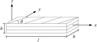
FIGURE 1. Geometry of a cross-ply laminated composite beam.

The beam is subjected to a transverse distributed loading $p_z$, respectively. Based on the higher-order theory for laminated composite plates introduced by Reddy (1984), the displacement field of an arbitrary point on the beam cross-section is given by

$u_1\left(x,z\right)=z\left[\psi \left(x\right)-\frac{4}{3}\frac{z^2}{h^2}\left(\psi \left(x\right)+\frac{\partial w\left(x\right)}{\partial x}\right)\right](1)$

$u_2\left(x,z\right)=0(2)$

$u_3\left(x,z\right)=w\left(x\right)(3)$

where $w\left(x\right)$ is the transverse displacement of the midplane ($z=0$); $\psi \left(x\right)$ is the rotation of a normal to the midplane, and $x$, $z$ are the axial and thickness coordinates of the beam.

Splitting the transverse displacement $w\left(x\right)$ into a bending $w_b\left(x\right)$ and a shear $w_s\left(x\right)$ component, i.e., Vo and Thai (2012).

$w\left(x\right)=w_b\left(x\right)+w_s\left(x\right)(4)$

and introducing the transformation

$\frac{\partial w_s\left(x\right)}{\partial x}=\psi \left(x\right)+\frac{\partial w\left(x\right)}{\partial x}\text{or}\psi \left(x\right)=-\left[\frac{\partial w\left(x\right)}{\partial x}-\frac{\partial w_s\left(x\right)}{\partial x}\right]=-\frac{\partial w_b\left(x\right)}{\partial x}(5)$

Equations 1–3 can be rewritten in the following form

$u_1\left(x,z\right)=-z\frac{\partial w_b\left(x\right)}{\partial x}-f\left(z\right)\frac{\partial w_s\left(x\right)}{\partial x}(6)$

$u_2\left(x,z\right)=0(7)$

$u_3\left(x,z\right)=w_b\left(x\right)+w_s\left(x\right)(8)$

where $f\left(z\right)=\frac{4}{3}\frac{z^3}{h^2}$. The displacement field given above yields the following nonzero components of the strain tensor

${\epsilon }_x=-z\frac{{\partial }^2{w}_b}{\partial x^2}-f\left(z\right)\frac{{\partial }^2{w}_s}{\partial x^2}(9)$

${\gamma }_{xz}=\left[1-\frac{df\left(z\right)}{dz}\right]\frac{\partial w_s}{\partial x}=\mathrm{g}\left(z\right)\frac{\partial w_s}{\partial x}(10)$

where $g\left(z\right)=\left(1-\frac{4z^2}{h^2}\right)$, and for reasons of brevity $w_b=w_b\left(x\right)$ and $w_s=w_s\left(x\right)$.

Substituting Eqs 9, 10 into the stress-strain relations for the kth lamina in the lamina coordinate we obtain (Khdeir and Reddy, 1997)

${\sigma }_x^{\left(k\right)}={\overline{Q}}_{11}^{\left(k\right)}{\epsilon }_x(11)$

${\tau }_{xz}^{\left(k\right)}={\overline{Q}}_{55}^{\left(k\right)}{\gamma }_{xz}(12)$

with ${\overline{Q}}_{11}^{\left(k\right)}$, ${\overline{Q}}_{55}^{\left(k\right)}$ being the well-known transformed elastic stiffnesses

${\overline{Q}}_{11}^{\left(k\right)}=Q_{11}^{\left(k\right)}{\cos }^4{\theta }_k+2\left(Q_{12}^{\left(k\right)}+2Q_{66}^{\left(k\right)}\right){\sin }^2{\theta }_k{\cos }^2{\theta }_k+Q_{22}^{\left(k\right)}{\sin }^4{\theta }_k(13)$

${\overline{Q}}_{55}^{\left(k\right)}=Q_{44}^{\left(k\right)}{\sin }^2{\theta }_k+Q_{55}^{\left(k\right)}{\cos }^2{\theta }_k(14)$

and $Q_{11}^{\left(k\right)}$, $Q_{12}^{\left(k\right)}$, $Q_{22}^{\left(k\right)}$, $Q_{44}^{\left(k\right)}$, and $Q_{55}^{\left(k\right)}$ are

$Q_{11}^{\left(k\right)}=\frac{E_1^{\left(k\right)}}{1-{\nu }_{12}^{\left(k\right)}{\nu }_{21}^{\left(k\right)}},Q_{12}^{\left(k\right)}=\frac{E_2^{\left(k\right)}{\nu }_{12}^{\left(k\right)}}{1-{\nu }_{12}^{\left(k\right)}{\nu }_{21}^{\left(k\right)}},Q_{22}^{\left(k\right)}=\frac{E_2^{\left(k\right)}}{1-{\nu }_{12}^{\left(k\right)}{\nu }_{21}^{\left(k\right)}}(15)$

$Q_{44}^{\left(k\right)}=G_{23}^{\left(k\right)},Q_{55}^{\left(k\right)}=G_{13}^{\left(k\right)},Q_{66}^{\left(k\right)}=G_{12}^{\left(k\right)}(16)$

while ${\theta }_k$ is the angle between the principal material axis and the coordinate $x$ axis.

Applying the Principle of Virtual Work

${\displaystyle {\int }_0^l{\displaystyle {\int }_A\left[{\sigma }_x^{\left(k\right)}\delta {\epsilon }_x+{\tau }_{xz}^{\left(k\right)}\delta {\gamma }_{xz}\right]dA}dx}-{\displaystyle {\int }_0^l\left[p_z\delta \left(w_b+w_s\right)\right]dx}=0(17)$

and substituting Eqs 9, 10 yields

$\begin{array}{r}{\displaystyle {\int }_0^l{\displaystyle {\int }_A\left\{{\sigma }_x^{\left(k\right)}\left[-z\frac{{\partial }^2\delta w_b}{\partial x^2}-f\left(z\right)\frac{{\partial }^2\delta w_s}{\partial x^2}\right]+{\tau }_{xz}^{\left(k\right)}g\left(z\right)\frac{\partial \delta w_s}{\partial x}\right\}dA}dx}\\ -{\displaystyle {\int }_0^l\left[p_z\left(\delta w_b+\delta w_s\right)\right]dx}=0\end{array}(18)$

Introducing now the following stress resultants

$M_b={\displaystyle {\int }_{A}z{\sigma }_x^{\left(k\right)}dA},M_s={\displaystyle {\int }_{A}f\left(z\right){\sigma }_x^{\left(k\right)}dA},Q={\displaystyle {\int }_A\mathrm{g}\left(z\right){\tau }_{xz}^{\left(k\right)}dA}(19)$

Eq. 18 become

${\displaystyle {\int }_0^l\left(-M_b\frac{{\partial }^2\delta w_b}{\partial x^2}-M_s\frac{{\partial }^2\delta w_s}{\partial x^2}+Q\frac{\partial \delta w_s}{\partial x}\right)dx}-{\displaystyle {\int }_0^l\left[p_z\left(\delta w_b+\delta w_s\right)\right]dx}=0(20)$

Integrating the appropriate terms in the above equation and collecting the coefficients of $\delta w_b$, and $\delta w_s$ we obtain the following governing equations

$\frac{{\partial }^2{M}_b}{\partial x^2}=-p_z(21)$

$\frac{{\partial }^2{M}_s}{\partial x^2}+\frac{\partial Q}{\partial x}=-p_z(22)$

together with the following associated boundary conditions of the form: specify

$w_b\text{or}{Q}_b\equiv \frac{\partial M_b}{\partial x}(23)$

$w_s\text{or}{Q}_s\equiv \frac{\partial M_s}{\partial x}+Q(24)$

$\frac{\partial w_b}{\partial x}\text{or}{M}_b(25)$

$\frac{\partial w_s}{\partial x}\text{or}{M}_s(26)$

Substituting Eqs 11, 12 into Eq. 19 and using Eqs 9, 10 yields the stress resultants in terms of the displacements as

$M_b=-D_{11}\frac{{\partial }^2{w}_b}{\partial x^2}-F_{11}\frac{{\partial }^2{w}_s}{\partial x^2}(27)$

$M_s=-F_{11}\frac{{\partial }^2{w}_b}{\partial x^2}-H_{11}\frac{{\partial }^2{w}_s}{\partial x^2},Q=A_{55}\frac{\partial w_s}{\partial x}(28)$

where

$D_{11}=b{\displaystyle {\int }_{-h/2}^{h/2}{\overline{Q}}_{11}^{\left(k\right)}{z}^{2}dz},F_{11}=b{\displaystyle {\int }_{-h/2}^{h/2}{\overline{Q}}_{11}^{\left(k\right)}zf\left(z\right)dz},H_{11}=b{\displaystyle {\int }_{-h/2}^{h/2}{\overline{Q}}_{11}^{\left(k\right)}{f}^2\left(z\right)dz}(29)$

$A_{55}=b{\displaystyle {\int }_{-h/2}^{h/2}{\overline{Q}}_{55}^{\left(k\right)}{g}^2\left(z\right)dz}(30)$

Finally, after the substitution of the stress resultants, Eqs 27, 28 into Eqs 21, 22, we arrive at the equilibrium equations in terms of the displacements

$-D_{11}\frac{{\partial }^4{w}_b}{\partial x^4}-F_{11}\frac{{\partial }^4{w}_s}{\partial x^4}=-p_z(31)$

$-F_{11}\frac{{\partial }^4{w}_b}{\partial x^4}-H_{11}\frac{{\partial }^4{w}_s}{\partial x^4}+A_{55}\frac{{\partial }^2{w}_s}{\partial x^2}=-p_z(32)$

which together with the pertinent boundary conditions (23)–(26) constitute the boundary value problem solved using the Analog Equation Method (AEM), a robust numerical method based on an integral equation technique (Katsikadelis and Tsiatas, 2003; Tsiatas et al., 2018).

Regression Models

In this work, several linear and nonlinear regression models are comparatively examined. Linear regression is a linear model that assumes a linear relationship between the input variables and the output variable, and the predicted value can be calculated from a linear combination of the input variables (Narula and Wellington, 1982). The distance from each data point to the predicted values is calculated and sum all these squared errors together. This quantity is minimized by the ordinary least squares method to estimate the optimal values for the coefficients of each independent variable.

There are extensions of the linear model called regularization methods. These methods seek to both minimize the sum of the squared error of the model on the training set but also to reduce the complexity of the model. Two popular regularization methods for linear regression are the Lasso Regression (Zou et al., 2007) where Ordinary Least Squares is modified to also minimize the absolute sum of the coefficients (L1 regularization), and the Ridge Regression (Hoerl et al., 1985) where Ordinary Least Squares is modified to also minimize the squared absolute sum of the coefficients (L2 regularization). A Bayesian view of ridge regression is obtained by noting that the minimizer can be considered as the posterior mean of a model (Tipping, 2001). The elastic net (Friedman et al., 2010) is a regularized regression method that linearly combines the L1 and L2 penalties of the lasso and ridge methods. Huber’s criterion is a hybrid of squared error for relatively small errors and absolute error for relatively large ones. Lambert-Lacroix and Zwald (2011) proposed Huber regressor to combine Huber’s criterion with concomitant scale and Lasso.

An L1 penalty minimizes the size of all coefficients and allows any coefficient to go to the value of zero, acting as a type of feature selection method since removes input features from the model. Least Angle Regression (Efron et al., 2004) is a forward stepwise version of feature selection for regression that can be adapted for the Lasso not to require a hyperparameter that controls the weighting of the penalty in the loss function since the weighting is discovered automatically by Least Angle Regression method via cross-validation. LassoLars is a lasso model implemented using the Least Angle Regression algorithm, where unlike the implementation based on coordinate descent, this yields the exact solution, which is piecewise linear as a function of the norm of its coefficients.

Orthogonal matching pursuit (Pati et al., 1993) tries to find the solution for the L0-norm minimization problem, while Least Angle Regression solves the L1-norm minimization problem. Although these methods solve different minimization problems, they both depend on a greedy framework. They start from an all-zero solution, and then iteratively construct a sparse solution based on the correlation between features of the training set and the output variable. They converge to the final solution when the norm approaches zero.

K Neighbors Regressor (KNN) algorithm uses feature similarity to predict the values of new instances (Altman, 1992). The distance between the new instance and each training instance is calculated, the closest k instances are selected based on the preferred distance and finally, the prediction for the new instance is the average value of the dependent variable of these k instances.

Unlike linear regression, Classification and Regression Tree (CART) does not create a prediction equation, but data are partitioned into subsets at each node according to homogeneous values of the dependent variable and a decision tree is built to be used for making predictions about new instances (Breiman et al., 1984). We can enlarge the tree until always gives the correct value in the training set. However, this tree would overfit the data and not generalize well to new data. The correct policy is to use some combination of a minimum number of instances in a tree node and maximum depth of tree to avoid overfitting.

The basic idea of Boosting is to combine several weak learners into a stronger one. AdaBoost (Freund and Schapire, 1997) fits a regression tree on the training set and then retrains a new regression tree on the same dataset but the weights of each instance are adjusted according to the error of the previous tree predictions. In this way, subsequent regressors focus more on difficult instances.

Random Forests algorithm (Breiman, 2001) builds several trees with the CART algorithm using for each tree a bootstrap replica of the training set with a modification. At each test node, the optimal split is derived by searching a random subset of size K of candidate features without replacement from the full feature set.

Like Random Forests, Gradient Boosting (Friedman, 2001) is an ensemble of trees, however, there are two main differences. Firstly, the Random forests algorithm builds each tree independently while Gradient Boosting builds one tree at a time since it works in a forward stage-wise manner, introducing a weak learner to improve the shortcomings of existing weak learners. Secondly, Random Forests combine results at the end (by averaging the result of each tree) while Gradient Boosting combines results during the process.

LightGBM (Ke et al., 2017) extends the gradient boosting algorithm by adding automatic feature selection and focusing on instances with larger gradients to speed up training and sometimes even improve predictive performance.

The Extra-Trees algorithm (Geurts et al., 2006) creates an ensemble of unpruned regression trees according to the well-known top-down procedure of the regression trees. The main differences concerning other tree-based ensemble methods are that the Extra-Trees algorithm splits nodes by choosing fully at random cut-points and that uses the whole learning set (instead of a bootstrap replica) to grow the trees.

Passive-Aggressive regressor (Crammer et al., 2006) is generally used for large-scale learning since it is an online learning algorithm. In online learning, the input data come sequentially, and the learning model is updated step-by-step, as opposed to batch learning, where the entire dataset is used at once.

Numerical Results and Discussion

The scope of the current study is to exploit predictive models for the maximum deflection $\max w$ of a symmetric cross-ply (${\theta }_1^{°}$/ ${\theta }_2^{°}$/ ${\theta }_3^{°}$) rectangular beam for various span-to-depth ratios and boundary conditions subjected to a uniformly distributed load $p_z$. All laminates are of equal thickness and made of the same orthotropic material. The main parameters that influence the response of the composite beams are the moduli of elasticity $E_1,E_2$, the span-to-depth $L=l/h$ and the ply angles ${\theta }_1^{°}$/ ${\theta }_2^{°}$/ ${\theta }_3^{°}$. The range of values of the parameters together with the material properties are given as: $E_1,E_2=\left\{\mathrm{1,2,3},\mathrm{...15}\right\}$, $G_{12}=G_{13}=0.5E_2$, $G_{23}=0.2E_2$, ${\nu }_{12}=0.25$, $L=l/h=\left\{\mathrm{1,2,3,4,5}\right\}$, ${\theta }_1,{\theta }_2=\left\{0,\pi /8,\pi /4, 3\pi /4,\pi /2\right\}$, and ${\theta }_1={\theta }_3$ (due to symmetry). For the given range of the parameters, Eqs 31, 32 are solved numerically producing a comprehensive database for each one of the examined boundary conditions presented in Table 1. This dataset contains $15\times 15\times 5\times 5\times 5=28125$ values of $\max w$ which are used in the regression analysis.

TABLE 1

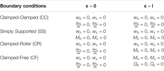
TABLE 1. Boundary conditions examined for the prediction of the maximum deflection $\max \overline{w}$.

A plethora of regression algorithms, presented in the previous section, were employed for building corresponding predictive models of the $\max w$ using pyCaret (Ali, 2020), which is an open-source software machine learning library. A 5-fold cross-validation resampling procedure was used for evaluating the performance of the predictive models. The dataset was randomly divided into five folds of equal size and each fold was used for evaluating the performance of the model trained on the rest folds, whereas the final measure was the average value of the computed evaluation metrics on each test fold. Evaluation metrics are a measure of how well a model performs. The most popularly used evaluation metrics for regression problems are the mean absolute error (MAE), the mean absolute percentage error (MAPE), the mean square error (MSE), the root mean square error (RMSE), the root mean squared log error (RMSLE) and the coefficient of determination. The lower the value of these metrics the better the model. The perfect value of metrics is 0, indicating that the prediction model is perfect. To quantify the accuracy of the examined algorithms, the following evaluation metrics are used herein:

Mean absolute error (MAE)

$\text{MAE}=\frac{1}{n}{\displaystyle \sum }_{i=1}^n|y{\prime }_i-y_i|(33)$

Mean absolute percentage error (MAPE)

$\text{MAPE}=\frac{1}{n}{\displaystyle \sum }_{i=1}^n\left(\left|y_i^{\prime }-y_i\right|\right)/\left|y_i^{\prime }\right|(34)$

Mean square error (MSE)

$\text{MSE}=\frac{1}{n}{\displaystyle \sum }_{i=1}^n{\left(y_i^{\prime }-y_i\right)}^2(35)$

Root mean square error ($\text{RMSE}$)

$\text{RMSE}=\sqrt{\frac{1}{n}{\displaystyle \sum }_{i=1}^n{\left(y_i^{\prime }-y_i\right)}^2}(36)$

Root mean squared log error ($\text{RMSLE}$)

$\text{RMSLE}=\sqrt{\frac{1}{n}{\displaystyle \sum }_{i=1}^n{\left(\log \left(y_i^{\prime }+1\right)-\text{log}(y_i+1)\right)}^2}(37)$

Coefficient of determination (${\text{R}}^2$)

${\text{R}}^2=\frac{S{S}_{reg}}{S{S}_{tot}}=\frac{{{\displaystyle \sum }}_j{\left(y_i^{\prime }-\overline{y}\right)}^2}{{{\displaystyle \sum }}_i{\left(y_i-\overline{y}\right)}^2},(38)$

where $y{\prime }_i$ refers to predicted values, and $y_i$ refers to true values. $S{S}_{reg}$ is the regression sum of squares (i.e., explained sum of squares), and $S{S}_{tot}$ is the total sum of squares, which is proportional to the variance of the data. The coefficient of determination (${\text{R}}^2$) is the square of the correlation between the actual and predicted variable and ranges from $0$ to $1$. A zero value indicates that the model cannot explain any of the predicted variables. A value of $1$ indicates that the regression model explains perfectly the predicted variable.

Apart from the evaluation metrics of the machine learning algorithms, two other useful tools are presented for the predictive analysis of the $\max w$. First, the feature importance is a technique for assigning scores to input features that indicate the relative importance of each feature for the prediction. The scores can highlight which features are most relevant to the target and the opposite, i.e., which features are the least relevant. Most importance scores are calculated using the most accurate predictive model that has been fit on our data (Louppe et al., 2013). Second, the correlation matrix heatmap illustrates the correlation dependence between the variables of the database. That is, each square of the matrix represents the correlation between the attributes paired on the two axes. A value of $+1$ (or $-1$) indicates a perfect correlation between two variables, with $+1$ indicating a positive correlation and $-1$ a negative (inverse) correlation; a value in the range from $0.6$ to $1$ (or from $-0.6$ to $-1$) indicates a strong correlation; a value between $0.4$ and $0.6$ (or between $-0.4$ and $-0.6$) indicates a moderate correlation; a value in the range from $0$ to $0.4$ (or from $0$ to $-0.4$) indicates a weak correlation.

Clamped-Clamped Beam

First, a clamped-clamped beam is analyzed. The evaluation metrics of the employed regression algorithms are tabulated in Table 2. The Extra-Trees Regressor algorithm is the most effective algorithm reaching a $R^2$ value of 0.9994, followed by the Random Forest Regressor and the Decision Tree Regressor. By examination of the evaluation metrics, it is obvious that there are significant differences in the effectiveness between algorithms. Nevertheless, the algorithms that perform best do so consistently for all problems, as will be demonstrated.

TABLE 2

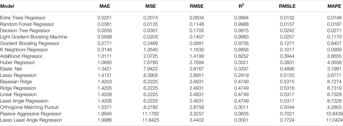
TABLE 2. Evaluation metrics for the clamped-clamped beam.

From the feature importance plot (see Figure 2A), it is observed that the most important parameters for predicting the target attribute $\max w$ is the modulus of elasticity $E_2$ and the span-to-depth ratio $L(=l/h)$. Next comes the ply angle $\text{th}1(={\theta }_1^{°})$ which is more important than $E_1$, and $\text{th}2(={\theta }_2^{°})$. Moreover, the correlation matrix heatmap has been evaluated for this problem; in this figure, the blue color indicates a negative correlation between the two parameters, while the red one indicates a positive correlation. Moreover, the intensity of the color implies how strongly these attributes are correlated, meaning that the deeper color corresponds to a stronger correlation. The correlation matrix heatmap of Figure 2B reveals that the maximum deflection is positively correlated with the parameters $L,$ ${\theta }_1^{°}$, ${\theta }_2^{°}$ and negatively correlated with $E_1$ and $E_2$. This means that increase of the span-to-depth ratio or increase of the angles of the plies leads to an increase of the maximum deflection. Conversely, an increase of either elastic moduli leads to a decrease in the maximum deflection. Nevertheless, $E_2$ is more strongly correlated with $\max w$ than $E_1$. Finally, the ply angle ${\theta }_1^{°}$ seems to be more important than the angle ${\theta }_2^{°}$ in making the beam stiffer, yet the difference is small.

FIGURE 2

FIGURE 2. (A) Feature importance plot and (B) correlation matrix heatmap for the clamped-clamped beam.

Simply Supported Beam

In this second example, a simply supported beam is analyzed. The Extra-Trees Regressor algorithm outperforms the other regression algorithms once again (see Table 3). The feature importance plot (see Figure 3A) shows an importance sequence different from that of the previous example. That is, the span-to-depth ratio $L\left(=l/h\right)$ is more important than the modulus of elasticity $E_2$, while the ply angle $\text{th}1(={\theta }_1^{°})$ is more important than $E_1$ and $\text{th}2(={\theta }_2^{°})$. Furthermore, the correlation matrix heatmap shown in Figure 3B reveals that, again, the maximum deflection is positively correlated with the parameters $L,$ ${\theta }_1^{°}$, ${\theta }_2^{°}$ and negatively correlated with $E_1$ and $E_2$. As previously, the correlation of $E_2$ is significantly stronger than that of $E_1.$ The ply angles exhibit weak positive correlations with the maximum deflection, with $\text{th}1(={\theta }_1^{°})$ being the prevailing one.

TABLE 3

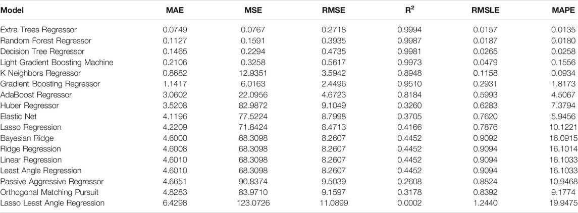
TABLE 3. Evaluation metrics for the simply supported beam.

FIGURE 3

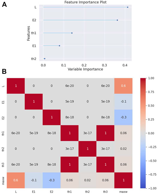
FIGURE 3. (A) Feature importance plot and (B) correlation matrix heatmap for the simply supported beam.

Clamped-Roller Beam

In this example, a clamped-roller beam is analyzed. In Table 4 it is shown that the Extra-Trees Regressor algorithm is again the most effective, as compared to the other regression algorithms. The feature importance plot (see Figure 4A) shows once more a similar to the clamped-clamped beam importance sequence. That is, the most important parameter is the modulus of elasticity $E_2$, followed closely by the span-to-depth ratio $L(=l/h)$. The ply angle $\text{th}1(={\theta }_1^{°})$ is more important than $E_1$, and $\text{th}2(={\theta }_2^{°})$. Furthermore, the correlation matrix heatmap shown in Figure 4B reveals that, again, the maximum deflection is positively correlated with the parameters $L,$ ${\theta }_1^{°}$, ${\theta }_2^{°}$ and negatively correlated with $E_1$ and $E_2$. The elastic modulus $E_2$ exhibits a stronger correlation with the maximum deflection than $E_1$. As in the case of the clamped-clamped beam, the ply angle ${\theta }_1^{°}$ is more important than the angle ${\theta }_2^{°}$.

TABLE 4

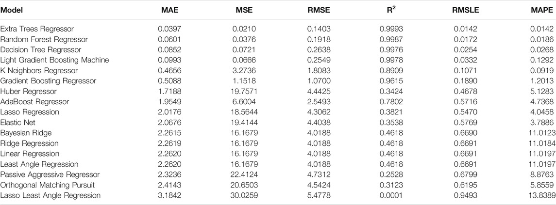
TABLE 4. Evaluation metrics for the clamped-roller beam.

FIGURE 4

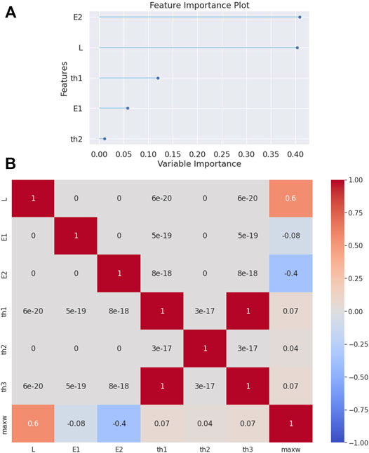
FIGURE 4. (A) Feature importance plot and (B) correlation matrix heatmap for the clamped-roller beam.

Clamped-free Beam

In the case of a clamped-free beam (cantilever), while the evaluation metrics designates once more the Extra-Trees Regressor algorithm superiority (see Table 5), the feature importance plot (see Figure 5A) presents a similar to the simply supported beam importance sequence. That is, the most important parameter is the span-to-depth ratio $L(=l/h)$ followed the modulus of elasticity $E_2$. The ply angle $\text{th}1(={\theta }_1^{°})$ is more important than $E_1$, and $\text{th}2(={\theta }_2^{°})$.

TABLE 5

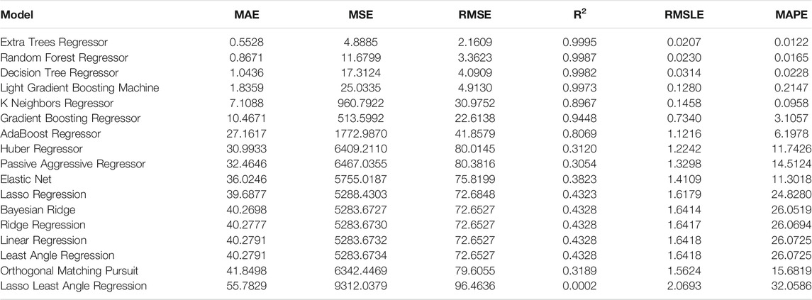
TABLE 5. Evaluation metrics for the clamped-free beam.

FIGURE 5

FIGURE 5. (A) Feature importance plot and (B) correlation matrix heatmap for the clamped-free beam.

The correlation matrix heatmap (see Figure 5B) again shows that the $\max w$ is positively correlated with the parameters $L,$ ${\theta }_1^{°}$, ${\theta }_2^{°}$ and negatively correlated with $E_1$ and $E_2$. In this case, the ply angle ${\theta }_1^{°}$ is significantly more strongly correlated with the maximum deflection than the angle ${\theta }_2^{°}$.

Friedman Ranking

Finally, to better assess the results obtained from each algorithm, the Friedman test methodology proposed by Demšar (2006) was employed for the comparison of several algorithms over multiple datasets (Table 6). As was expected, the Extra-Trees Regressor algorithm is the most accurate in our case. A simple computational tool, written in JAVA programming language using Weka API (Hall et al., 2009) along with the relevant data, is provided to the interested reader as Supplementary Data to this article.

TABLE 6

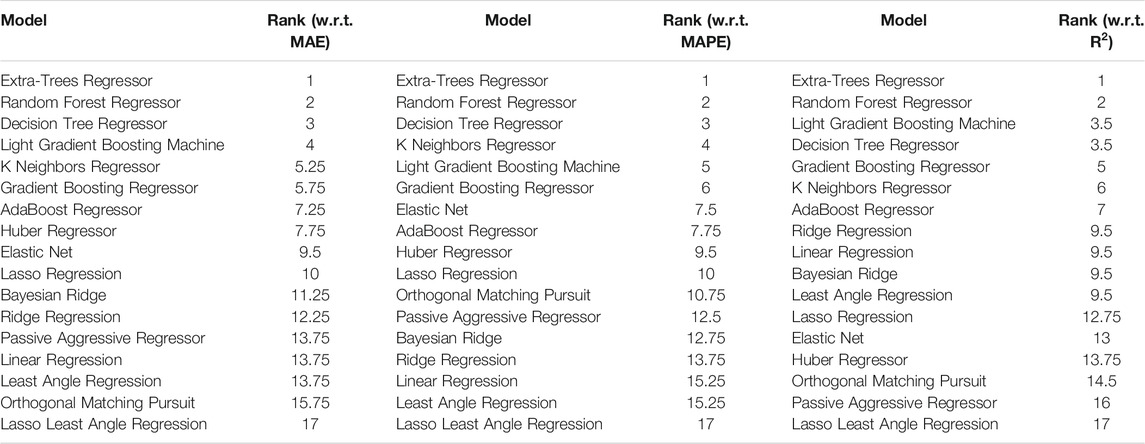
TABLE 6. Friedman ranking.

Conclusion

In this paper, several machine learning regression models were employed for the prediction of the deflection of symmetric laminated composite beams subjected to a uniformly distributed load. Training, validation, and testing of the models require large amounts of data that cannot be provided by the scarce experiments. Instead, ample amounts of data are generated numerically using a refined higher-order beam theory for various span-to-depth ratios and boundary conditions, by appropriate discretization of all pertinent geometric and material properties.

The main conclusion that can be drawn from this investigation are as follows:

• Regarding the regression models, the Extra-Trees algorithm is, without doubt, the best performer for all cases of boundary conditions, followed by the Random Forest Regressor, the Decision Tree Regressor, the Light Gradient Boosting Machine, and the K Neighbors Regressor.

• The prediction errors of the best-performing models are adequately small for engineering purposes. This allows for the rapid design of the composite beams without resolving to a mathematical implementation of higher-order beam theories. Moreover, these models can be integrated into modern metaheuristic optimization algorithms which use only payoff data (i.e., no derivative data) to allow for the fast and reliable optimization of such beams.

• Regarding the relative importance of the design variables for the evaluation of the deflection, the span-to-depth ratio and the modulus of elasticity $E_2$ are unambiguously the most important features. The next level of importance includes the angle ply ${\theta }_1$ and the modulus of elasticity $E_1$. Surprisingly, the angle ${\theta }_2$ is the least important variable.

• The span-to-depth ratio $L$ has the strongest positive correlation to the target attribute $\max w$ for all cases of boundary conditions, as evidenced by the correlation matrices. In all cases, the maximum deflection is positively correlated with the parameters $L,$ ${\theta }_1$, ${\theta }_2$ and negatively correlated with $E_1$ and $E_2$.

• An easy-to-use computational tool has been implemented which is provided as Supplementary Material to the present article.

Data Availability Statement

The original contributions presented in the study are included in the article/Supplementary Material, further inquiries can be directed to the corresponding author.

Author Contributions

GT had the research idea, drafted the article, and contributed to the theoretical formulation of the beam theory. SK and AC contributed to the conception and design of the work, and the theoretical analysis of the regression techniques. The manuscript was written through the contribution of all authors. All authors discussed the results, reviewed, and approved the final version of the manuscript.

Conflict of Interest

The authors declare that the research was conducted in the absence of any commercial or financial relationships that could be construed as a potential conflict of interest.

Publisher’s Note

All claims expressed in this article are solely those of the authors and do not necessarily represent those of their affiliated organizations, or those of the publisher, the editors and the reviewers. Any product that may be evaluated in this article, or claim that may be made by its manufacturer, is not guaranteed or endorsed by the publisher.

Supplementary Material

The Supplementary Material for this article can be found online at: https://www.frontiersin.org/articles/10.3389/fbuil.2022.855112/full#supplementary-material

References

Ali, M. (2020). PyCaret: An Open-Source, Low-Code Machine Learning Library in Python. Available at: https://www.pycaret.org

Google Scholar

Altman, N. S. (1992). An Introduction to Kernel and Nearest-Neighbor Nonparametric Regression. The Am. Statistician 46, 175–185. doi:10.1080/00031305.1992.10475879

CrossRef Full Text | Google Scholar

Bickford, W. B. (1982). A Consistent Higher Order Beam Theory. Dev. Theor. Appl. Mech. 11, 137–150.

Google Scholar

Breiman, L., Friedman, J. H., Olshen, R. A., and Stone, C. J. (1984). Classification and Regression Trees. New York, NY: Routledge. doi:10.1201/9781315139470

CrossRef Full Text | Google Scholar

Breiman, L. (2001). Random Forests. Mach. Learn. 45, 5–32. doi:10.1023/A:1010933404324

CrossRef Full Text | Google Scholar

Civalek, Ö., and Kiracioglu, O. (2010). Free Vibration Analysis of Timoshenko Beams by DSC Method. Int. J. Numer. Meth. Biomed. Engng. 26, 1890–1898. doi:10.1002/CNM.1279

CrossRef Full Text | Google Scholar

Crammer, K., Dekel, O., Keshet, J., Shai, S.-S., and Singer, Y. (2006). Online Passive-Aggressive Algorithms. J. Mach. Learn. Res. 7, 551–585.

Google Scholar

Demšar, J. (2006). Statistical Comparisons of Classifiers over Multiple Data Sets. J. Mach. Learn. Res. 7, 1–30.

Google Scholar

Efron, B., Hastie, T., Johnstone, I., Tibshirani, R., Ishwaran, H., Knight, K., et al. (2004). Least Angle Regression. Ann. Statist. 32, 407–499. doi:10.1214/009053604000000067

CrossRef Full Text | Google Scholar

Eisenberger, M. (2003). An Exact High Order Beam Element. Comput. Structures 81, 147–152. doi:10.1016/S0045-7949(02)00438-8

CrossRef Full Text | Google Scholar

Endo, M. (2016). An Alternative First-Order Shear Deformation Concept and its Application to Beam, Plate and Cylindrical Shell Models. Compos. Structures 146, 50–61. doi:10.1016/J.COMPSTRUCT.2016.03.002

CrossRef Full Text | Google Scholar

Freund, Y., and Schapire, R. E. (1997). A Decision-Theoretic Generalization of On-Line Learning and an Application to Boosting. J. Comput. Syst. Sci. 55, 119–139. doi:10.1006/JCSS.1997.1504

CrossRef Full Text | Google Scholar

Friedman, J., Hastie, T., and Tibshirani, R. (2010). Regularization Paths for Generalized Linear Models via Coordinate Descent. J. Stat. Soft. 33, 1. doi:10.18637/jss.v033.i01

PubMed Abstract | CrossRef Full Text | Google Scholar

Friedman, J. H. (2001). Greedy Function Approximation: A Gradient Boosting Machine. Ann. Stat. 29, 1189–1232. doi:10.1214/aos/1013203451

CrossRef Full Text | Google Scholar

Geurts, P., Ernst, D., and Wehenkel, L. (20062006). Extremely Randomized Trees. Mach. Learn. 63, 3–42. doi:10.1007/S10994-006-6226-1

CrossRef Full Text | Google Scholar

Hall, M., Frank, E., Holmes, G., Pfahringer, B., Reutemann, P., and Witten, I. H. (2009). The WEKA Data Mining Software. SIGKDD Explor. Newsl. 11, 10–18. doi:10.1145/1656274.1656278

CrossRef Full Text | Google Scholar

Heyliger, P. R., and Reddy, J. N. (1988). A Higher Order Beam Finite Element for Bending and Vibration Problems. J. Sound Vibration 126, 309–326. doi:10.1016/0022-460X(88)90244-1

CrossRef Full Text | Google Scholar

Hoerl, A. E., Kennard, R. W., and Hoerl, R. W. (1985). Practical Use of Ridge Regression: A Challenge Met. Appl. Stat. 34, 114–120. doi:10.2307/2347363

CrossRef Full Text | Google Scholar

Katsikadelis, J. T., and Tsiatas, G. C. (20032003). Large Deflection Analysis of Beams with Variable Stiffness. Acta Mechanica 164, 1–13. doi:10.1007/S00707-003-0015-8

CrossRef Full Text | Google Scholar

Ke, G., Meng, Q., Finley, T., Wang, T., Chen, W., Ma, W., et al. (2017). LightGBM: A Highly Efficient Gradient Boosting Decision Tree. Adv. Neural Inf. Process. Syst. 30. Available at: https://github.com/Microsoft/LightGBM (Accessed December 14, 2021).

Google Scholar

Khdeir, A. A., and Reddy, J. N. (1997). An Exact Solution for the Bending of Thin and Thick Cross-Ply Laminated Beams. Compos. Structures 37, 195–203. doi:10.1016/S0263-8223(97)80012-8

CrossRef Full Text | Google Scholar

Lambert-Lacroix, S., and Zwald, L. (2011). Robust Regression through the Huber’s Criterion and Adaptive Lasso Penalty. Electron. J. Statist 5, 1015–1053. doi:10.1214/11-EJS635

CrossRef Full Text | Google Scholar

Liew, K. M., Pan, Z. Z., and Zhang, L. W. (2019). An Overview of Layerwise Theories for Composite Laminates and Structures: Development, Numerical Implementation and Application. Compos. Structures 216, 240–259. doi:10.1016/J.COMPSTRUCT.2019.02.074

CrossRef Full Text | Google Scholar

Lin, X., and Zhang, Y. X. (2011). A Novel One-Dimensional Two-Node Shear-Flexible Layered Composite Beam Element. Finite Elem. Anal. Des. 47, 676–682. doi:10.1016/J.FINEL.2011.01.010

CrossRef Full Text | Google Scholar

Louppe, G., Wehenkel, L., Sutera, A., and Geurts, P. (2013). Understanding Variable Importances in Forests of Randomized Trees. Adv. Neural Inf. Process. Syst. 26, 431–439.

Google Scholar

Murthy, M. V. V. S., Roy Mahapatra, D., Badarinarayana, K., and Gopalakrishnan, S. (2005). A Refined Higher Order Finite Element for Asymmetric Composite Beams. Compos. Structures 67, 27–35. doi:10.1016/J.COMPSTRUCT.2004.01.005

CrossRef Full Text | Google Scholar

Narula, S. C., and Wellington, J. F. (1982). The Minimum Sum of Absolute Errors Regression: A State of the Art Survey. Int. Stat. Rev./Revue Internationale de Statistique 50, 317. doi:10.2307/1402501

CrossRef Full Text | Google Scholar

Nguyen, T.-K., Nguyen, N.-D., Vo, T. P., and Thai, H.-T. (2017). Trigonometric-Series Solution for Analysis of Laminated Composite Beams. Compos. Structures 160, 142–151. doi:10.1016/J.COMPSTRUCT.2016.10.033

CrossRef Full Text | Google Scholar

Pati, Y. C., Rezaiifar, R., and Krishnaprasad, P. S. (1993). “Orthogonal Matching Pursuit: Recursive Function Approximation with Applications to Wavelet Decomposition,” in Conf. Rec. Asilomar Conf. Signals, Syst. Comput., Pacific Grove, CA, November 1–3, 1993 1, 40–44. doi:10.1109/ACSSC.1993.342465

CrossRef Full Text | Google Scholar

Pawar, E. G., Banerjee, S., and Desai, Y. M. (2015). Stress Analysis of Laminated Composite and Sandwich Beams Using a Novel Shear and Normal Deformation Theory. Lat. Am. J. Sol. Struct. 12, 1340–1361. doi:10.1590/1679-78251470

CrossRef Full Text | Google Scholar

Reddy, J. N. (1984). A Simple Higher-Order Theory for Laminated Composite Plates. J. Appl. Mech. 51, 745–752. doi:10.1115/1.3167719

CrossRef Full Text | Google Scholar

Srinivasan, R., Dattaguru, B., and Singh, G. (2019). Exact Solutions for Laminated Composite Beams Using a Unified State Space Formulation. Int. J. Comput. Methods Eng. Sci. Mech. 20, 319–334. doi:10.1080/15502287.2019.1644394

CrossRef Full Text | Google Scholar

Tipping, M. E. (2001). Sparse Bayesian Learning and the Relevance Vector Machine. J. Mach. Learn. Res. 1, 211–244.

Google Scholar

Tsiatas, G. C., Siokas, A. G., and Sapountzakis, E. J. (2018). A Layered Boundary Element Nonlinear Analysis of Beams. Front. Built Environ. 4, 52. doi:10.3389/FBUIL.2018.00052/BIBTEX

CrossRef Full Text | Google Scholar

Vo, T. P., and Thai, H.-T. (2012). Static Behavior of Composite Beams Using Various Refined Shear Deformation Theories. Compos. Structures 94, 2513–2522. doi:10.1016/J.COMPSTRUCT.2012.02.010

CrossRef Full Text | Google Scholar

Wang, C. M., Reddy, J. N., and Lee, K. H. (2000). Shear Deformable Beams and Plates : Relationships with Classical Solutions. Elsevier.

Google Scholar

Zou, H., Hastie, T., and Tibshirani, R. (2007). On the “Degrees of freedom” of the Lasso. Ann. Stat. 35, 2173–2192. doi:10.1214/009053607000000127

CrossRef Full Text | Google Scholar