A Nature-Based Solution for Coastal Protection: Wind Tunnel Investigations on the Influence of Sand-Trapping Fences on Sediment Accretion

Introduction

Coastal dunes are present along sandy coastlines worldwide and have various functions, such as contributing to biodiversity, socioeconomic services including nature conservation, recreation, and tourism, and natural flood protection for the low-lying hinterland against storm surges (van Thiel de Vries, 2009; Hesp, 2011; de Vries, 2013; Keijsers et al., 2015). Coastal dunes also act as sediment resources in case of erosive storm events; the sediments can naturally shift and move to the beach or nearshore areas and dissipate wave energy and, thus, mitigate erosion (van Thiel de Vries, 2009). Aeolian sediment transport processes from the beach toward the coastal dunes increase coastal dune volumes, while marine processes, which predominately occur during storm surges, lead to dune erosion (Hesp, 2011). However, along with aeolian sediment transport marine processes can also contribute to foredune growth along dissipative coastlines. The highest dune growth rates are often observed during winter months, when the beach is eroding, at the highest wind velocities, and high water levels (Cohn et al., 2018; 2019). Due to the rise in the sea level caused by climate change, it is currently assumed that erosion processes will accelerate and land loss will increase as well (Harff et al., 2011; Hesp, 2011; Keijsers et al., 2015). In addition, socioeconomic pressure in coastal areas is increasing (NASA, 2020). In order to address the challenges in coastal protection and at the same time respond to people’s growing environmental awareness, there is a great need for nature-based solutions that aim to use natural processes and resources. Since sand-trapping fences are part of nature-based solutions, they are commonly installed along sandy coastlines along with barrier island systems to strengthen coastal dunes and increase the flood protection level (Li and Sherman, 2015; Itzkin et al., 2020a; Eichmanns et al., 2021). They cause a local reduction in wind velocity, leading to downwind sediment accumulation around the fences (Hotta and Horikawa, 1990; Li and Sherman, 2015; Lawlor and Jackson, 2021). The functions of sand-trapping fences in coastal areas vary and thus, range from rehabilitating eroded areas such as blowouts in coastal dunes, strengthening coastal dune toe establishment, preventing sand drifting from protectable infrastructures, limiting human access to nature, or initiating the formation of coastal dunes through selective sand deposition (O'Connel,; Adriani and Terwindt, 1974; Gerhardt, 1990; Li and Sherman, 2015; Eichmanns and Schüttrumpf, 2021). For detailed information about sand-trapping fences, refer to Eichmanns et al. (2021).

Generally, it is found that using sand-trapping fences at the seaward side of the dune leads to an increased foredune growth rate compared to no fenced areas (Jackson and Nordstrom, 2011; Eichmanns and Schüttrumpf, 2021). This additional sediment buffer can protect coastal dunes by attenuating wave energy (Ruz and Anthony, 2008; Itzkin et al., 2020b). However, the application of such sand-trapping fences can impair the sediment supply for the beaches and landward coastal dunes and create a physical boundary for the natural movement of fauna. Subsequently, a less dynamic beach–dune system affects the beach width and, therefore, the coastal protection against coastal erosion (Itzkin et al., 2020a). Wider beaches generally offer greater coastal protection against erosion than smaller beaches (Itzkin et al., 2020b). Thus, sand-trapping fences influence the natural topography of coastal dunes and present vegetation (Gallego-Fernández, 2013). For example, Itzkin et al. (2020a) found that coastal dunes are typically shorter, wider, and smaller in volume than natural foredunes in non-fenced and undeveloped areas. However, this may also be explained because fences tend to be installed close to more vulnerable coastal dunes, which are usually smaller.

Numerous studies consider the wind and turbulence field behind porous fences with variable geometry (height and length) (Mulhearn and Bradley, 1977; Ning et al., 2020), porosity (Perera, 1981; Hotta and Horikawa, 1990; Lee and Kim, 1999; Dong et al., 2007), opening size (Manohar and Bruun, 1970; Lee and Kim, 1999), incoming wind velocity, or wind turbulence (Dong et al., 2007; Yu et al., 2020). It is found that fence porosity and fence height are the predominant influencing factors on the wind field and, thus, the sand-trapping efficiency (Li and Sherman, 2015). However, recommendations on the fence height and porosity of sand-trapping fences in coastal areas are commonly based on empirical practice (Li and Sherman, 2015; Eichmanns et al., 2021). Thus, the correlation of sand-trapping efficiency as a function of, for example, fence porosity and fence height is needed.

In this study, indoor wind tunnel experiments were carried out to study the wind regime and sand-trapping efficiency of sand-trapping fences with different fence porosities and fence heights. The objective is to evaluate different fence porosities and fence heights influencing trap efficiency. Therefore, the following research goals were set:

1) Investigation of the influence of fence height and fence porosity on the wind regime.

2) Investigation of reproducibility of the sediment accretion around a single sand-trapping fence.

3) Considering the model effetcs on the sediment accretion around a single sand-trapping fence.

4) Evaluation of trap efficiency of a single sand-trapping fence over time.

5) Investigation of the influence of fence porosity on trapping sediment.

6) Giving general recommendations on fence properties.

Materials and Methods

Experimental Design

Physical model tests were conducted on sand-trapping fences with different heights and porosities in an indoor subsonic, blowing-sand wind tunnel at the Institute of Hydraulic Engineering and Water Resources Management (IWW), Rheinisch Westfälische Hochschule (RWTH) Aachen University, Germany. Fence porosity and grain size distribution of the sediment is based on in situ measurements conducted in Langeoog and Norderney, where the influence of sand-trapping fences on the dune toe growth and its relation with potential aeolian sediment transport was already investigated by the authors (see Eichmanns and Schüttrumpf, 2020, 2021).

For this work, a wind tunnel was built by the IWW itself and was constructed mainly from wooden panels, except the test section was built from polymethylmethacrylate to allow visual observation of the experiments. The wind tunnel had a total length of L = 25.8 m, see Figure 1. The cross-sectional area was H = 1.0 m (height) and B = 0.58 m (width). The wind tunnel consisted of the following four parts: the power section with the wind machine, rectifier section followed by contraction section, channel with test section, and diffusion section. A sediment bed with a length of l = 4 m, a width of b = 0.4 m, and a depth of t = 0.15 m was installed in the test section. The sand-trapping fence as the focus of the investigation was installed within the sediment bed, d = 2 m from the edge of the sediment bed in the windward direction. In addition, a sediment source with a layer with a volume of V = 0.0435 m³ was placed about 1 m behind the roughness section in the main wind direction.

FIGURE 1

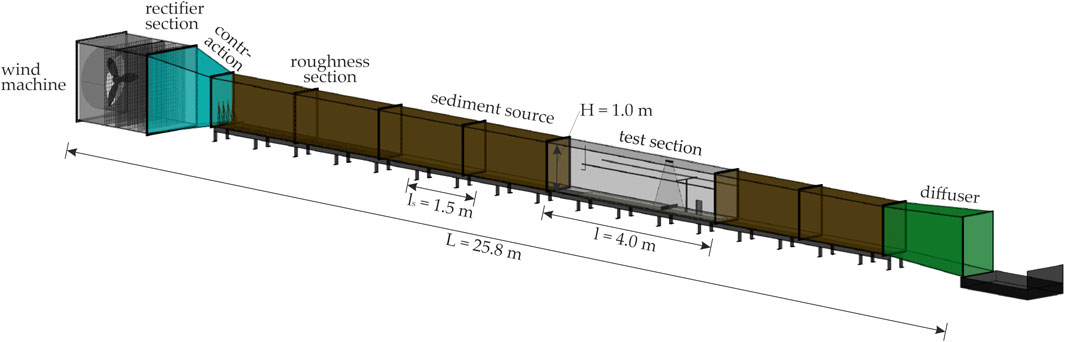
FIGURE 1. Subsonic, blowing-sand wind tunnel built at IWW, RWTH Aachen University, Germany.

The Trotec TTW (Trotec) wind machine generates a continuous airflow of Q = 45.600 m³/h. The wind machine is equipped with an inverter that allowed mean wind velocities to be adjusted between u_mean ∼ 1–10 m/s. The wind first passes through a honeycomb, see Figure 2A, and second, through a coarser and a finer screen, see Figure 2B, to straighten the airflow. The honeycomb is designed following the findings of Barlow et al. (1999) and Mehta (1979) and was built out of ∼7.500 bounded polyvinylchloride tubes with an outer diameter of d = 16 mm and a length of l = 120 mm. In addition, the surface roughness is increased by four spires, a trip fence, and a 6-m-long artificial grass cover, see Figure 2C.

FIGURE 2

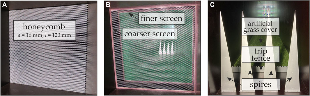
FIGURE 2. (A) Honeycomb and (B) coarser and finer screens to straighten the airflow in the main wind direction, and (C) spires, trip fence, and an artificial grass cover to increase the surface roughness.

Experimental Setup

The flow field and sediment flux measurements were conducted separately. First, a fixed sediment surface was installed to measure the wind velocities via a hot-wire anemometer. Since the hot-wire anemometer is susceptible to damages from the windblown sediment, a thin layer of sediment glued to a wooden panel was installed while measuring the wind profiles in the test section. Only wind directions perpendicular to the fences were investigated in the wind tunnel. The experimental mean wind velocities were u₁ = 6.1 m/s, u₂ = 7.4 m/s, and u₃ = 9.3 m/s. Then a moveable sediment bed combined with a sediment source was established, where a vertical sediment trap determined the sediment flux and a 2D LiDAR sensor SICK LMS4000, the sediment accretion around the sand-trapping fence. This fixed and moveable sediment bed procedure was already carried out in comparable wind tunnel experiments such as Hotta and Horikawa (1990). A GoPro Hero 8 recorded each experiment for visual observation. In Figure 3, the instrumentation setup for the test section is shown.

FIGURE 3

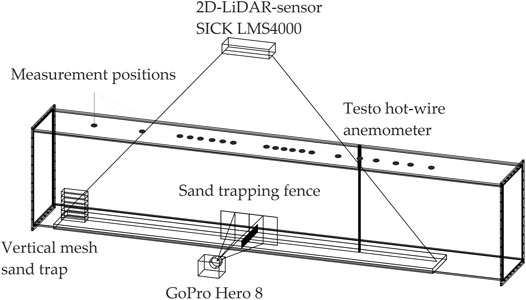
FIGURE 3. Instrumentation setup for the test section, including 2D LiDAR sensor SICK LMS4000, Testo hot-wire anemometer for the different measurement positions, vertical mesh sand trap, and GoPro Hero 8.

The sediment source is added, such as in experiments by Creyssels et al. (2009) or Ho et al. (2011, 2012), to favor the development of a steady state of saltation. Experiment’s duration is set to t = 10 min to ensure almost stationary sediment fluxes. This is in agreement with other investigations such as Chen et al. (2019, 2020), Wang et al. (2018), or Miri et al. (2019), where short measuring intervals, up to several minutes, are common. Some of these experiments were even shorter. Exceeding this experiment duration would empty the sediment source and the sediment bed. Furthermore, vertical mesh sand traps are limited to a constant sand-trapping capacity that will exceed if testing times are excessive. Moreover, we wanted to avoid the effects of supply limitations on the dune development (Swann et al., 2015) or increase the model effects at the physical boundaries (transition from wooden panels to the sediment bed).

Sediment from the study site Norderney was used for the experiments. To ensure the defined moisture content of M < 0.1%, for all investigations, the sediment was dried in a dry oven at a temperature of around T = 105°C. According to the specifications in DIN EN ISO 14688-1 (2018), a sedimentological analysis was conducted. The median grain size of the sediment was d₅₀ ∼ 212 µm.

The investigated sand-trapping fences were modeled using locally available brushwood branches with a diameter of d ∼ 2–10 mm. In total, nine different fence configurations were investigated in the wind tunnel, varying in both fence height (h = 40, 80, 120 mm) and fence porosity (ε ∼ 20–58%). The two-dimensional porosity was determined as the open to total surface ratio. The exact porosities are shown in Figure 4 and were determined by evaluating photographs of the sand-trapping fences. Therefore, the photographs were processed with the MATLAB, 2018’s (R2018b, version 9.510.944444) Color Thresholder Application. The areas overlaid by the brushwood branches were identified and colored in black with a chosen threshold value. The contrast toward the background was increased and colored in white to indicate that there is no brushwood. For more information about the segmentation of the photographs, refer Eichmanns and Schüttrumpf (2021).

FIGURE 4

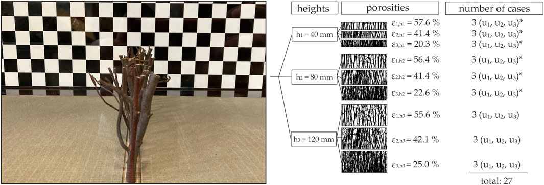
FIGURE 4. Modeling nine different sand-trapping fences with changing fence heights and fence porosities and showing the number of cases investigated (*only wind profiles were measured).

The porosity of the different sand-trapping fence configurations varies slightly over height due to the uneven nature of the branches. Thus, the modeled fences tend to become a little more porous in their upper parts. In the following, the mean porosity is determined for the three different fence heights and used for low (ε₁ = 22.6%), medium (ε₂ = 41.6%), and high (ε₃ = 56.5%) porosity. The mean porosities generally correspond to the porosities of Langeoog and Norderney’s sand-trapping fences (Eichmanns and Schüttrumpf, 2021). However, the brushwood bundles differ in their stem characteristics, such as the stem diameter (d ∼ 2–10 mm). At present, the authors are not aware that the stem diameter significantly influences the sediment accretion around the sand-trapping fence, especially since, in a scientific research, the fence’s porosity was identified as a significant influence on trapping sediments (e.g., Arens et al., 2001; Zhang et al., 2010; Li and Sherman, 2015; Miri et al., 2019; Yu et al., 2020).

To measure the wind fields, all fence heights and porosities were investigated (27 cases); to measure the sediment accretion around the sand-trapping fence, only the highest fence height was installed (nine cases), see also Figure 4. Researching this fence height ensures that the saltation layer height does not significantly exceed the fence height, allowing the fence to capture most of the windblown sediment, see also Sediment Transport Fluxes. The influence would be more remarkable for other fence heights since the fence heights are considerably lower than the saltation layer height, and thus, the aeolian sediment would also blow over the fence.

Similarity to Nature and Compliance with Physical Model Laws

The type of aerodynamic flow in the wind tunnel can be characterized by the Mach number M (-), as follows

$\text{M}=\frac{\text{u }}{c} ,(1)$

where c ∼ 343 m/s (temperature T = 20°C) is the speed of sound of the medium. At any point in the wind tunnel, the velocity is less than the speed of sound of the air (M < 1), and thus it is a subsonic flow (Barlow et al., 1999; Anderson, 2017). The thickness of the boundary layer in the test section was determined to be approximately $\text{δ}$ ∼ 650 mm. Incompressible airflows are primarily characterized by their Reynolds number and are decisive for their dynamic similarity. The following conditions must be met: Reynolds number of the flow must be greater than Re_flow >10⁵ and the roughness Reynolds number must be greater than Re_R > 2.5 (Barlow et al., 1999; Cattafesta et al., 2010). The Reynolds number of the flow is defined as follows:

$R{e}_{flow}=\frac{u_{\infty }\cdot \text{ δ}}{\text{ν}},(2)$

where u_∞ (m/s) is the free flow velocity in front of the test section and ν ∼ 1.516·10⁻⁵ m²/s (T = 20°C) is the kinematic viscosity of air (White, 1996; Barlow et al., 1999; Cattafesta et al., 2010). The roughness Reynolds number Re_R (-) is defined as follows:

$R{e}_R=\frac{z_0\cdot u_{\ast }}{\text{ν}} ,(3)$

where u_* (m/s) is the shear velocity and z₀ (mm) is the aerodynamic roughness length (Nikuradse, 1933; Vithana, 2013), see also Measurement of Wind Velocity Characteristics. The first criterion was achieved with Re_flow ∼ 3 × 10⁵, whereas the roughness Reynolds number was not achieved. The roughness Reynolds number could only be determined for experiments with the immobile sand bed, as the sensitive hot-wire probe could otherwise be destroyed by saltating sediment grains. However, we assumed that the roughness Reynolds number independence was achieved during experiments with the moveable sediment bed because the saltation process generally increases the roughness Reynolds number (Cermak, 1987; White, 1996; Barlow et al., 1999).

The minimal entrance length L_in,min ∼ 10–25·$\text{δ}$ (m) for describing the logarithmic wind profile is considered sufficiently long with L_in = 15 m under the assumption that saltation is present and the Froude criterion Fr (-) is fulfilled, as follows:

$Fr = \frac{u_{\infty }}{\sqrt{g·H}},(4)$

where g = 9.81 m/s² is the gravitational acceleration and H (m) is the wind tunnel height. The smaller the Froude number, the faster a constant shear stress velocity, and thus, a constant velocity profile is achieved during saltation (White, 1996). The Froude criterion is fulfilled for the investigated flow velocities u_1–3 = 6.1–9.3 m/s with Fr << 20 (Owen and Gillette, 1985). Sidewall effects are not expected with the investigated low wind velocities and corresponding shear stress velocities in the wind tunnel. For the blockage ratio two criteria exist. The maximum blockage ratio BR₁ (-) defined as

$B{R}_1= \frac{A_{fence}}{A}\stackrel{!}{<} 0.1 ,(5)$

which is fulfilled for fence models with heights h₁ = 40 mm and h₂ = 80 mm, whereas the blockage ratio BR₂ (-) can only be met for the lowest fence height h₁ = 40 mm. It is defined as the ratio of the fence height h (mm) to the height of the boundary layer δ (mm):

$B{R}_2= \frac{h}{\text{δ}}\stackrel{!}{<} \mathrm{0.15.}(6)$

These criteria were not always met in past studies either, such as Dong et al. (2007), Wang et al. (2018), and Yu et al. (2020), but assumed to have a minor influence as long as the fence height was at least smaller than the height of the boundary layer. Since the selected fence heights are considerably smaller than the boundary layer height, it can be assumed that no significant influence is expected by exceeding this limit value.

Measurement of Wind Velocity Characteristics

The Testo hot-wire anemometer (testo, 2021), equipped with an external data logger Testo 440 dp, was placed in the center of the wind tunnel at predefined heights (z = 3, 6, 12, 24, 40, 80, 120, 200, and 250 mm) above the surface to measure wind velocities. For this purpose, the hot-wire anemometer was inserted via a hole in the wind tunnel cover, and after measurement of the wind profile, the anemometer was moved to the next position downwind. The respective holes in the lid were sealed tightly with plugs, see Figure 3. For the flow field test, the wind velocity profiles near the sand-trapping fence were measured on the leeward side at a distance of 2, 5, 8, 10, 12, 15, and 20 h from the fence, on the windward side at distances of −2h, −5h, and −10h, and at a reference position over the wooden panel at x = −2,200 mm from the fence, where h is the height of the sand-trapping fence. We recorded a steady and uniform airflow field in the test section without a sand-trapping fence, see also Figure 7. The hot-wire anemometer has an accuracy of ±0.03 m/s and 3% of the mean wind velocity. In order to obtain reliable measurement results, the measurement duration is decisive. A measurement duration that is too short can lead to incorrect measurement results. The longer the measurement duration, the more representative the measurement results. The wind velocity was measured for 10 min at two locations and then analyzed. The 10-min measurement period is divided into ten intervals of equal time (t = 1 min), and the difference between the mean flow velocity over each 1-min interval over the whole 10-min interval is determined. The maximum difference was ±1.2%. Therefore, a measurement interval of 1 min is defined as sufficiently accurate for this investigation. Moreover, the reproducibility of the measured data for the wind profiles was ensured by repeating several measurements randomly with a maximum deviation of ±4% at one measuring point.

An appropriate analytical approach to describe the wind velocity distribution over the viscous sub boundary layer for aerodynamically rough surfaces is the law of the wall, which is valid for neutral atmospheric stability conditions, as follows (Bagnold, 1954):

$u_z=\frac{u_{\text{*}}}{\mathrm{ĸ}}\cdot \mathit{ln}\frac{z}{z_0},(7)$

where u_z (m/s) is the wind velocity at height z (m) and κ (−) is the Kármán constant (here 0.41) (Nikuradse, 1933; Vithana, 2013). Figure 5 exemplifies the velocity profiles for u₁ = 6.1 m/s, u₂ = 7.4 m/s, and u₃ = 9.3 m/s at the reference position with corresponding shear velocities u_1* = 0.21 m/s, u_2* = 0.25 m/s, and u_3* = 0.28 m/s, and coefficient of determination R² = 0.95–0.98 is shown. It describes the approaching airflow entering the test section.

FIGURE 5

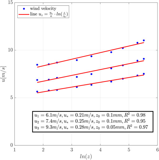
FIGURE 5. Examples of the velocity profile for u₁ = 6.1 m/s, u₂ = 7.4 m/s, and u₃ = 9.3 m/s. The blue dots represent the measured wind velocity and the red lines indicate the regression lines, see Eq. 7.

For all measurement heights at the reference position, the corresponding standard deviations were less with σ_min = 0.19 m/s, σ_max = 0.61 m/s, and σ_mean = 0.39 m/s, respectively.

When a particular critical value of drag and lift force on the sediment grain is exceeded, sediment transport is initiated. This is the so-called critical shear stress u_*t (18):

$u_{\ast t}=\text{A }\cdot \sqrt{\left(\frac{{\rho }_s}{{\rho }_a}-1\right)\cdot \text{ g }\cdot d_{50}} .(8)$

The empirical constant is given with A (-) (here 0.11), the density of air is given with ρ_a (kg/m³) (here 1.2 kg/m³), and the density of sediment grains with ρ_s (kg/m³) (here 2,650 kg/m³). The empirical constant considers the effect of cohesion; however, the influence of the protective layer of shells or moisture contents is not taken into account (Shao and Lu, 2000; Han et al., 2011; van Rijn and Strypsteen, 2019). The critical shear velocity was calculated for the wind tunnel investigations as u_*t = 0.24 m/s. However, it was noted that sediment transport occurred with critical shear velocities above u_*t = 0.20 m/s.

To describe the influence of different fence porosities and fence heights on the wind profile at a certain height z (mm) and distance x (mm) from the fence, the wind reduction coefficient R_c (-) is used (Cornelis and Gabriels, 2005; Wang et al., 2018; Yu et al., 2020):

$R_c=1-\frac{u_{x,z}}{u_{0_{x,z}}}.(9)$

The horizontal wind velocity is given with u_x,z (m/s) and the horizontal wind velocity at that exact position without any fence with u_0x,z (m/s). A high value indicates a high wind reduction.

Measurement of Sediment Flux

For each experimental mean wind velocity, mean sediment transport rates were measured to determine the incoming sediment flux from the sediment source. Thus, vertical mesh sand traps constructed according to Sherman et al. (2014) and already used in field experiments of Eichmanns and Schüttrumpf (2020), covering a height of z = 0.3 m above the surface, see Figure 3, were used. The vertical mesh sand trap consists of six rectangular aluminum tubes arranged one above the other. One rectangular aluminum tube has the dimensions of 0.1 m (width) × 0.05 m (height) × 0.25 m (length) and 2 mm (edges). One rectangular aluminum tube is equipped with a nylon monofilament with opening sizes of size = 50 µm. The vertical mesh sand traps were exposed to sediment flow during the defined time interval of t = 10 min, and, afterward, the collected sand was weighed per height. The empirical exponential decay function is used to describe the vertical distribution of sediment transport as follows (Ellis et al., 2009; Poortinga et al., 2014):

$q_z=q_0 \cdot \exp (-\text{β }\cdot \text{ z}),(10)$

where q_z (kg/m²/s) is the sediment transport rate at a predefined height z (m), q₀ (kg/m²/s) is the extrapolated saltating sediment mass transport at the surface, and the decay rate ß (1/m) is a constant to describe the vertical concentration gradient. A regression analysis of the experimental data gives the parameters ß and q₀ (Bauer and Davidson-Arnott, 2014). According to the scientific literature, the range of values for the fitting coefficient can vary significantly due to the weak correlation to physical aeolian parameters such as grain size or shear velocity (Bauer and Davidson-Arnott, 2014). Integrating Eq. 10 gives the total mass transport, as follows:

$Q_s={\int }_0^{\infty }{q}_z\cdot dz=\frac{q_0}{\beta } .(11)$

The total mass transport by saltation is given as Qs (kg/m/s) (Bauer and Davidson-Arnott, 2014). Since aeolian sediment transport is highly variable spatially and temporally, the experiments were repeated three times and the average value was used for further analysis (Baas and Sherman, 2006; Bauer and Davidson-Arnott, 2014; Strypsteen, 2019; van Rijn, 2019).

Measurement of Sand Accretion Around Sand-Trapping Fence Configurations

We deployed a 2D LiDAR scanner at the centerline of the wind tunnel, where the wind velocity profiles were also measured. We found that the centerline represents the sediment accretion around the sand-trapping fence well based on the camera recordings. The laser scanner detected the sediment surface elevations every Δt = 2 min with a systematic error of ±1.5 mm and a statistical error of ±2.5 mm (distances between 1.97–2.40 m). The measuring frequency was set to 10 Hz, and the angular resolution was 0.0833°.

In the following, the trap efficiency is used to evaluate the different sediment accretions around the configurations of the sand-trapping fence. In order to eliminate model effects on the sediment accretion caused by the fence, the sediment fluxes were distinguished based on the continuity equation. Thus, Figure 6 presents a schematic side view of the wind tunnel test section with the sediment accretion around the fence at timestep t₀ = 0 min and t₅ = 10 min. The yellow areas show the typical erosion areas, whereas the colored areas in orange give the accretion areas. The zero-crossing between two sediment surface elevations at different timesteps is defined as boundary condition distinguishing between the different sediment changes (sf₂, sf₃, and sf₄), see red crosses in Figure 6.

FIGURE 6

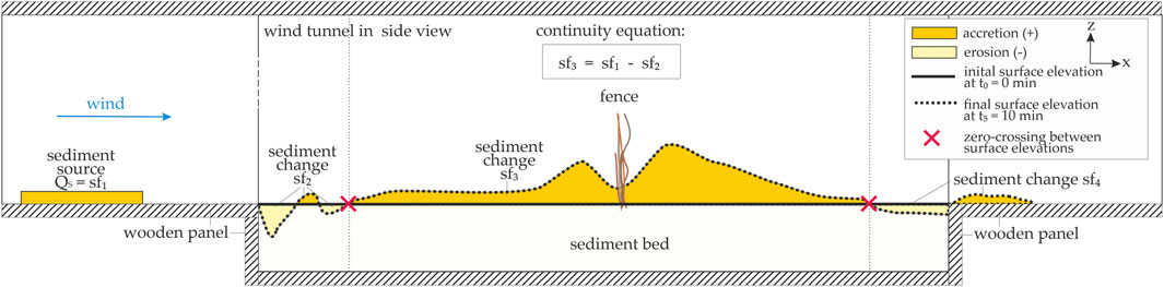
FIGURE 6. Two-dimensional side view of the wind tunnel test section showing the different sediment fluxes schematically: sf₁–sf₄ for determining the trapped sediment, see Eq. 13.

During the experiments, local scouring always occurred at the transition between the wooden panel and sediment bed and vice versa, see Sediment Accretion Around the Sand-Trapping Fence Configurations. These sediment changes sf₂ and sf₄ were caused by increasing shear stress associated with increasing surface roughness, which lead to fluctuations and turbulences, thus, initiating erosion processes (Swann et al., 2015). Since in a steady-state equilibrium, foredunes generally oscillate about a geomorphic equilibrium, accreting (recovery) and eroding (response), it is assumed that the scour sf₄ at the end of the sediment bed would extend over a longer distance followed by a sediment accretion (Swann et al., 2015). Thus, this sediment change sf₄ is excluded from further analysis. Excluding the sediment flux sf₄ (sf₄ << sf₃) still provides valid results.

It is assumed that during the experimental time frame of t = 10 min, the scours have a minor effect on the accretion of sediment around the sand-trapping fence. According to experiments of Hotta and Horikawa (1990) and Ning et al. (2020), the zero-crossing between two surface elevations at different timesteps shifts insignificantly toward the fence (maximum x/h ∼ 2) such as in our experiments. Thus, it is assumed that the morphodynamics around the sand-trapping fence is modeled correctly in our experiments, see also Sediment Accretion Around the Sand-Trapping Fence Configurations. However, this can only be determined adequately with a sufficiently long wind tunnel and extensive test durations.

For evaluating the sand-trapping of different fence configurations, the trap efficiency E (-), see for example, Ning et al. (2020) or Chen et al. (2019), is defined as follows:

$E=\frac{{\text{Q}}_t}{{\text{Q}}_s} .(12)$

The trapped sediment transport Q_t (kg/m/s) is estimated as the product of the bulk density of the sediment γ (kg/m³) and the cross-sectional dune area ΔA (m²) (sediment change sf₃) in the time interval Δt (s), as follows:

${\text{Q}}_t=\frac{\gamma · \Delta A}{\Delta t} .(13)$

The sediment transport for initiating the sediment accretion around the sand-trapping fence is calculated based on total mass transport Q_s, see Eq. 11, from which the sediment change sf₂ is subtracted. The bulk density was γ = 1,550 kg/m³ (average out of three measurements).

Since windblown sediment transport is highly variable both spatially and temporally, the experiments were repeated three to four times (Baas and Sherman, 2006; Bauer and Davidson-Arnott, 2014; van Rijn, 2019).

Results

Wind Velocity Characteristics

Figure 7A presents the flow field in the x-direction (mm) over the height z (mm) without a sand-trapping fence; Figures 7B–D depicts the flow fields in the vicinity of a sand trapping. The free mean velocity was u₃ = 9.3 m/s, and the x-axis and the y-axis were normalized by the fence height. The black dots represent the measurement positions of a hot-wire anemometer with the mean wind velocity values over the 1-min measuring interval, and the brown lines indicate the fence. Generally, the airflow slows down on the upwind side of the fence. Above the fence, the airflow accelerates, and on the leeward side, the vertical eddy zone occurs, resulting from the difference of the wind velocity above and through the fence.

FIGURE 7

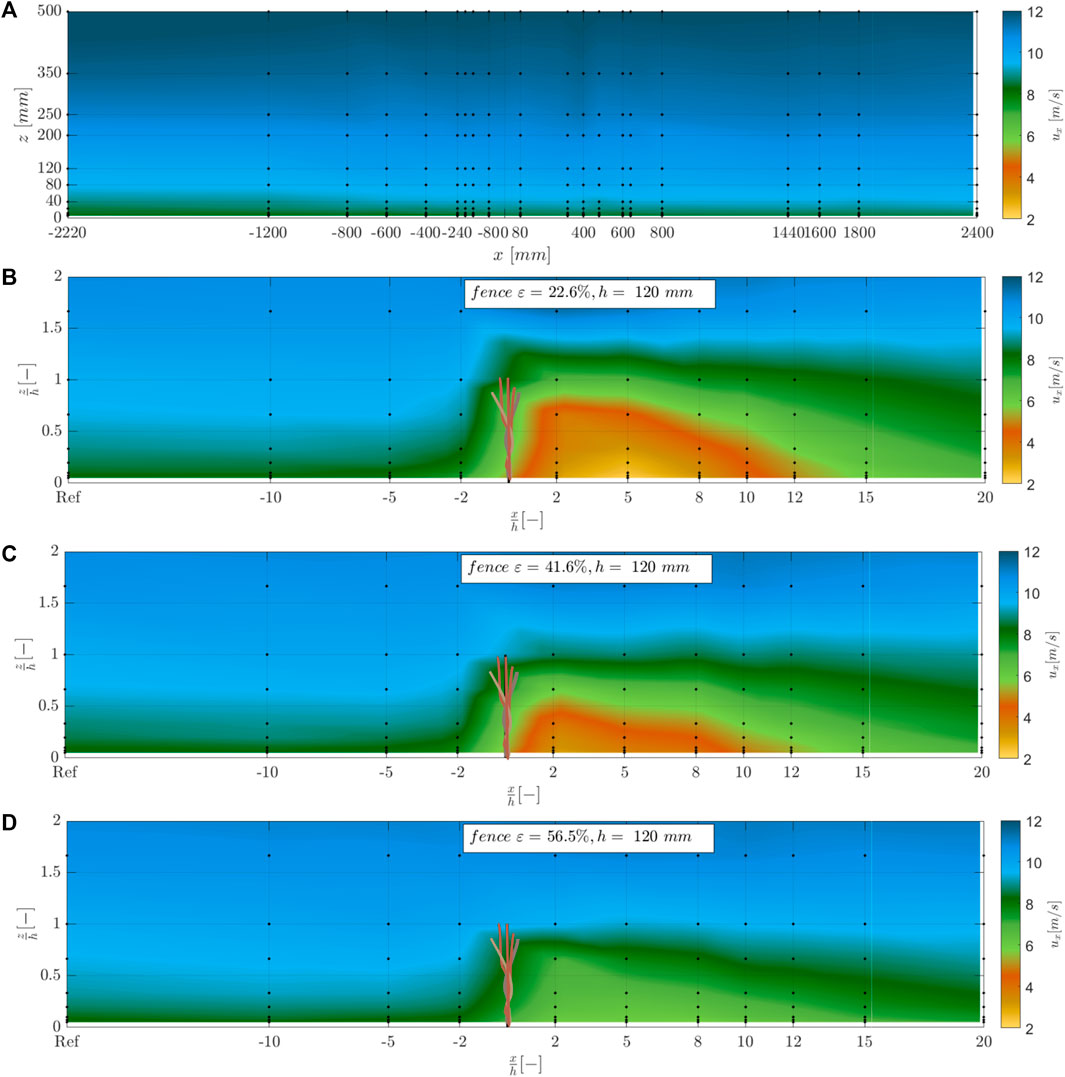
FIGURE 7. Flow fields (A) without a sand-trapping fence (B) in the vicinity of a sand-trapping fence at x/h = 0 with h₃ = 120 mm and (B) a porosity of ε₁ = 22.6%, (C) ε₂ = 41.6%, and (D) ε₃ = 56.6%. The free mean wind velocity was u₃ = 9.3 m/s. The black dots show the measuring locations of the hot-wire anemometer, and the brown lines indicate the sand-trapping fence.

The complexity of the airflow fields decreased while the fence porosity increased. For the low porosity fence, the wind velocity profiles show a higher range of measured wind velocities between u = 2.3–11.3 m/s than the high porosity fence profiles showing wind velocities between u = 6.3–11.1 m/s. In addition, the wind velocities in front of and behind the fence are reduced to a greater extent. For better illustration, Figure 8 represents the mean wind velocities in the x-direction for the different fence configurations, divided into the following fence heights: (A) h₁ = 40 mm (B) h₂ = 80 mm, and (C) h₃ = 120 mm. The mean wind velocity in the x-direction was averaged by values of wind velocities at heights of z = 3, 6, 12, 24, 40, 80, 120, 200, and 250 mm. The mean wind velocities were averaged up to a height of z = 250 mm within the boundary layer rather than the entire wind tunnel height of H = 1,000 mm.

FIGURE 8

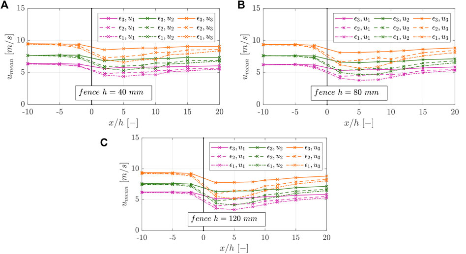
FIGURE 8. Mean wind velocity u₁–u₃ in the x-direction of fences with different characteristics ε₁–ε₃, divided into (A) the fence heights h₁ = 40 mm (B) h₂ = 80 mm, and (C) h₃ = 120 mm.

Comparing the wind fields for the different fence heights (h₁ = 40 mm, h₂ = 80 mm, and h₃ = 120 mm), we detected no significant differences in the mean wind velocities under constant porosity and constant free wind velocity.

For the lowest fence porosity (ε₁ = 22.6%) and the highest fence height (h₃ = 120 mm), the wind reduction is most significant at position x/h = 5. For the mean free wind velocity u₁ = 6.1 m/s, the lowest mean wind velocity in the x-direction was u_mean = 3.4 m/s, whereas for the lowest fence height (h₁ = 40 mm) and the lowest fence porosity (ε₁ = 22.6%), the lowest mean wind velocity was u_mean = 4.4 m/s at position x/h = 5. In the downwind direction, the wind velocity increased, reached their minimum at position x/h = 5, and then increased again to the initial wind velocity. For all fences with the characteristics of ε₂ = 41.6%, the minimum value was already reached at position x/h = 2. The higher the porosity of the fence was, the earlier the initial wind velocity of the fence was reached in the free stream.

Sediment Transport Fluxes

Figure 9 exemplifies the vertical distribution of sediment transport fluxes obtained from the vertical mesh sand traps for the wind velocity u₃ = 9.3 m/s. We found that sediment was mainly caught in heights of less than z ≤ 0.05 m for all wind velocities studied. This finding is in agreement that most sediment transport in coastal areas occurs for z < 0.05 m above the surface (Strypsteen, 2019). No sediment was caught in heights over z > 0.15 m, so the saltation layer height does not significantly exceed the fence height (h₃ = 120 mm), see Experimental Setup.

FIGURE 9

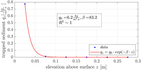
FIGURE 9. Vertical distribution of sediment transport flux obtained from the vertical mesh sand trap for wind velocity u₃ = 9.3 m/s and the best fit exponential decay function for experiment No. 3.3.

Table 1 presents the results of the trapped sediment from the vertical mesh sand traps with the total mass flux Qs (kg/m/s), the decay rate ß (1/m), the extrapolated saltating sediment mass transport at the surface q₀ (kg/m²/s), and the correlation coefficients R² (-) of the regression analysis. The measuring duration was t = 10 min. The transport fluxes varied between Qs = 0.005–0.078 kg/m/s for wind velocities ranging between u₁ = 6.1 m/s and u₃ = 9.3 m/s. For the lowest wind velocity u₁ = 6.1 m/s, the total mass fluxes show larger fluctuations than those at higher wind velocity u₂ = 7.4 m/s and u₃ = 9.3 m/s.

TABLE 1

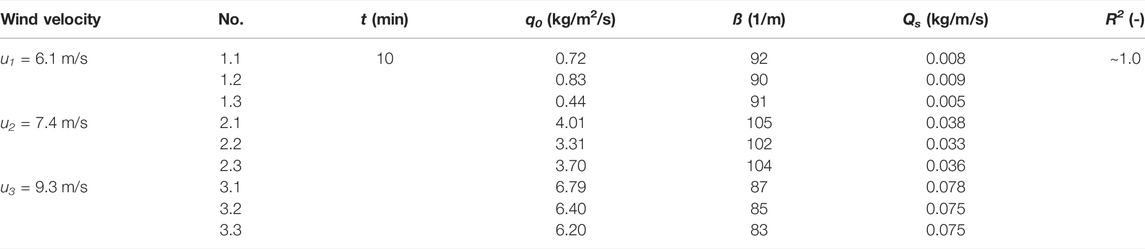
TABLE 1. Total mass flux results over the measuring duration, decay rate, extrapolated saltating sediment mass transport at the surface, and correlation coefficients of the vertical sediment profile regression analysis.

The regression parameters varied between ß = 83–105/m and q₀ = 0.44–6.79 kg/m²/s, indicating that the higher the wind velocity, the higher the extrapolated saltating sediment mass transport at the surface and the amount of the total sediment transport rate. However, the decay rate and the sediment transport height did not vary significantly during the experiments for different wind velocities.

Sediment Accretion Around the Sand-Trapping Fence Configurations

Figure 10 shows sediment accretion around the investigated sand-trapping fences h₃ = 120 mm over time, starting at t₀ = 0 min and ending at t₅ = 10 min. Both the x-axis (-) and the y-axis (-) are normalized over the fence height. The results for the investigated wind velocity u₁ = 6.1 m/s are shown in Figures 10A,D,G, u₂ = 7.4 m/s in Figures 10B,E,H, and u₃ = 9.3 m/s in Figures 10C,F,I, respectively. The first row shows the results for ε₁ = 22.6%, the second row for ε₂ = 41.6%, and the third row for ε₃ = 56.5%. The different colors of the lines indicate the different timesteps Δt = 2 min. The sediment changes are Δsf₂ and Δsf₃ is given in the legend.

FIGURE 10

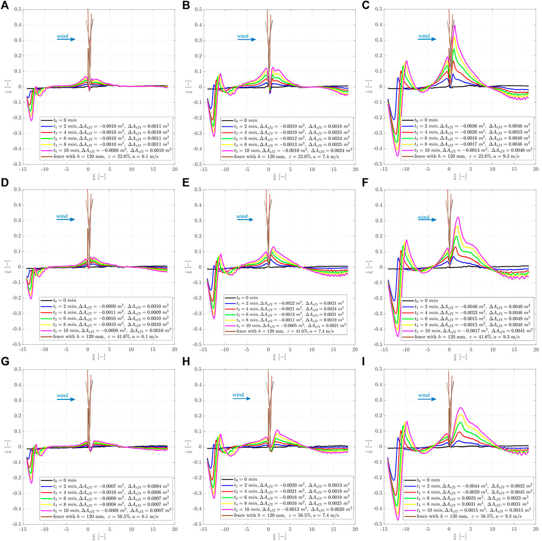
FIGURE 10. Sediment accretion around a porous fence h = 120 mm varying in fence porosity and investigated wind velocity. The first row (A-C) shows the results for ε₁ = 22.6%, the second row (D-F) for ε₂ = 41.6%, and the third row (G-I) for ε₃ = 56.5%. The first columns show u₁ = 6.1 m/s, the second column u₂ = 7.4 m/s, and the third column u₃ = 9.3 m/s.

The sediment accretion occurred predominantly horizontally and vertically, which corresponds to the first phase of dune growth, see for example Ning et al. (2020). Longer experiment durations would probably lead to the sediment accretion according to the second dune growth phase with almost exclusive horizontal dune growth if a sufficient sediment supply is provided. It is well seen that the higher the investigated wind velocity, the higher the total amount of deposited sediment at the sand-trapping fence at a given time, caused by a higher aeolian sediment transport rate. Furthermore, the denser the fence porosity, the higher the deposited sediment on the windward side of the sand-trapping fence at any given time. For example, for the lowest fence porosity of ε₁ = 22.6%, the deposited sand reached a height of maximum z/h ∼ 0.4, whereas for the highest fence porosity of ε₃ = 56.5%, the maximum height of z/h = 0.28 was reached. Generally, it can be recognized that for fences with ε₂ = 41.6% and ε₃ = 56.5%, scouring occurred in the main wind direction directly behind the fence at position x/h ∼ 1, whereas for ε₁ = 22.6%, only little scouring was recorded at this position.

The sediment accretion on the leeward side developed simultaneously but faster than the sediment accretion on the windward side of the fence. For the lower and middle wind velocities (u₁, u₂), the height of the sediment accretion of the windward side is approximately the same as the height of the leeward side of the fence. For the fence with the lowest porosity, the sediment accretion on the leeward side of the fence occurred until x/h ∼ six to eight, whereas fence with the medium porosity until x/h ∼ seven to nine and for the most porous fence until x/h ∼ 8–12.

Discussion

Regarding the similarity of the physical model tests to nature, it must be taken into account that some influencing factors such as non-stationary wind conditions, attacking wind direction, moisture, salt content of the sediment, shell fragments, the presence of vegetation, or the topography cannot be modeled in the wind tunnel experiments adequately. For example, the main wind direction was modeled solely orthogonal and onshore to the fence that does not correspond to nature. In nature, the wind forces attack the fence from all wind directions. However, wind directions play a significant role in controlling the apparent fetch length, which refers to the continuous increase in sediment transport rates with increasing fetch length downwind until an equilibrium condition is reached (critical fetch length) (Jackson and Cooper, 1999; Bauer and Davidson-Arnott, 2003). When estimations of aeolian sediment transport rates from the beach toward the coastal dunes are made, they are often divided into longshore and cross-shore sediment fluxes, see for example Nickling and Davidson Arnott, (1990). Furthermore, in nature, the presence of vegetation generally increases the surface roughness, favoring sediment deposition and dune formation (Adriani and Terwindt, 1974; Hacker et al., 2012; Keijsers et al., 2015; Cohn et al., 2019; Miri et al., 2019). The presence of vegetation and the natural formation of coastal dunes also influence the sand-trapping efficiency of sand-trapping fences and may superimpose or interact with them (Houser et al., 2015). Generally, moisture content of sediment strongly affects aeolian sediment transport. With increasing moisture content the cohesion is increasing leading to lower sediment transport rates. In our investigations the sediment was dried before testing, leading to higher sediment transport rates compared to nature (Davidson-Arnott et al., 2005; van Rijn and Strypsteen, 2019). However, these influencing factors, which are usually subject to strong spatial and temporal fluctuations, have a decisive influence on the sediment accretion around sand-trapping fences in nature. The standardized wind tunnel investigations, on the other hand, offer the great possibility to observe the influence of certain fence properties under constant boundary conditions. The influence of other factors, such as the natural dune formation, can thus be eliminated, allowing us to evaluate the effeciency of sand-trapping fences in a standardized manner.

Wind Velocity Characteristics

The wind profile could be measured well and provide reproducible data in repeated experiments with the applied methodology. In Figure 11, the wind reduction factors R_u (-), according to Eq. 9, for the fence heights h = 40, 80, 120 mm are shown along the x-axis, normalized over the fence heights.

FIGURE 11

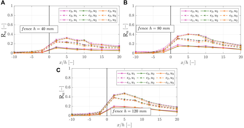
FIGURE 11. Wind reduction coefficients accordingly to Eq. 9 in the x-direction of fences with different characteristics, which are divided into (A) the fence heights h₁ = 40 mm (B) h₂ = 80 mm, and (C) h₃ = 120 mm.

In Figure 12, the wind reduction factors R_u (-) for the fence porosities of ε = 22.6, 41.6, 56.5% are shown respectively.

FIGURE 12

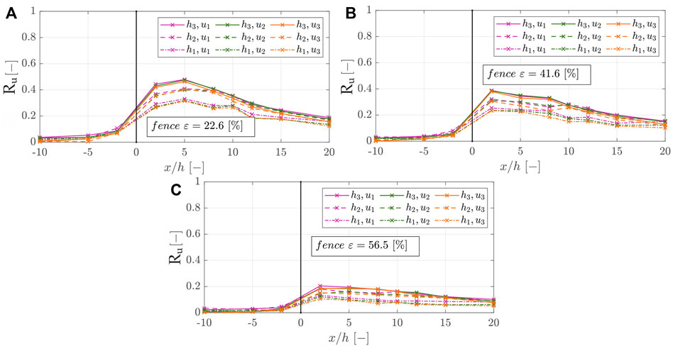
FIGURE 12. Wind reduction coefficients accordingly to Eq. 9 in the x-direction of fences with different characteristics, which are divided into (A) the fence porosities ε₁ = 22.6%, (B) ε₂ = 41.6%, and (C) ε₃ = 56.5%.

Note that a higher wind reduction factor indicates a more substantial reduction in wind velocity and thus favors sediment deposition around the sand-trapping fence. We recognized that the wind reduction coefficients were almost the same for varying free wind velocities but varied significantly for different fence porosities and fence heights. The results show that, with increasing distance from the fence, the wind reduction coefficient increased to the maximum value and then decreased or stabilized again. The position at which R_u begins to decrease or stabilize, the protection range, generally lies between x/h = 2–5. The wind reduction coefficient was substantially greater for higher fences (R_u,max = 0.48) than lower fences (R_u,max = 0.21) and also higher for less porous fences (R_u,max = 0.48) than for more porous fences. Furthermore, it becomes clear that for the medium and high fences, the influence of the porosity is greater than for the low fences since the variety of R_u is also smaller. However, the fence height plays a minor role in the case of the most porous fence. This is in agreement with findings of Perera (1981), who found in wind tunnel experiments with vertical and horizontal slats (porosity >30–50%) or Lee and Kim (1999) who found with perforated fences (circular openings with porosity >40%), no recirculating zone occurred due to the strong bleed flow. For ε₁ = 22.6% and ε₂ = 41.6%, the typical airflow conditions around a single porous fence can be identified (Plate, 1971). However, for the fence of porosity ε₃ = 56.5%, a strong bleed flow leads to smaller wind velocity reduction, the recirculating zone disappears, and the airflow zones become less complex (Dong et al., 2007).

Sediment Transport Fluxes and Sediment Accretion Around the Sand-Trapping Fence Configurations

We found that the two-dimensional development of the sediment accretion around the sand-trapping fences could be measured well with the 2D LiDAR scanner and is quantitatively reproducible in repeated experiments (maximum standard deviation of the sediment accretion σ ∼ 0.15). However, for low wind speeds, the ratio of the measurement error to the deposition heights is so small that the measurement error has a significant influence on the results. In addition, the aeolian sediment fluxes showed large temporal fluctuations, which were noticed especially during experiments with the wind velocity u₁ = 6.1 m/s, see Table 1. As far as the authors know, the reproducibility of the sediment accretion around a sand-trapping fence is investigated for the first time with the results presented herein.

Figure 13A gives the changes of cross-sectional area and Figure 13B the trap efficiency for all configurations over time. The changes of cross-sectional areas ΔA (m²) and the trap efficiencies E (-) are shown as the average value of three up to four repeated measurements. Generally, as the sediment transport rates increase, the cross-sectional areas around the sand-trapping fence also increase; with the densest fence tending to accumulate the most sediment, then the medium-density fence, and then the porous fence. At the beginning of the experiments, the trap efficiency increases, and as time passes, the efficiency decreases or stabilizes.

FIGURE 13

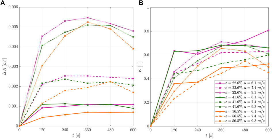
FIGURE 13. Change of (A) cross-sectional area ΔA (-) and (B) trap efficiency E (-) for different investigated fence configurations varying in fence porosities ε₁ = 22.6%, ε₂ = 41.6%, and ε₃ = 56.5% for investigated wind velocities u₁ = 6.1 m/s, u₂ = 7.4 m/s, and u₂ = 9.3 m/s expressed over the experiment duration t (s).

For the medium (u₂ = 7.4 m/s) and high wind velocity (u₃ = 9.3 m/s), the maximum trap efficiency is reached between t = 360–600 s, whereas, for the lowest wind velocity (u₁ = 6.1 m/s), the maximum is reached at t = 360 s. After the trap efficiency increases to its maximum, it decreases slightly or stagnates to equilibrium during the time investigated in our experiments. This is in accordance with findings of Ning et al. (2020), where the sand-trapping is highest at the beginning of the first phase, drops significantly until the end of the first phase, and continues to drop slowly until the end of the second phase.

For the different investigated sand-trapping fence’s porosities (ε₁ = 22.6%, ε₂ = 41.6%, ε₃ = 56.5%) and wind velocities (u₁ = 6.1 m/s, u₂ = 7.4 m/s, u₃ = 9.3 m/s), the calculated trap efficiencies, see Eq. 12, are shown as boxplots (Figure 14). Since the efficiencies vary over time, all timesteps of the experiments are included showing the variations. The mean trap efficiencies for the dense fence (ε₁ = 22.6%) E_h120,e22.6 are 0.69 (u₁ = 6.1 m/s), 0.57 (u₂ = 7.4 m/s), 0.63 (u₃ = 9.3 m/s) and for the medium fence E_h120,e41.6 are 0.66 (u₁ = 6.1 m/s), 0.52 (u₂ = 7.4 m/s), 0.58 (u₃ = 9.3 m/s). For the highest fence porosity (ε₃ = 56.5%), the efficiencies E_h120,e56.6 are 0.45 (u₁ = 6.1 m/s), 0.41 (u₂ = 7.4 m/s), 0.52 (u₃ = 9.3 m/s).

FIGURE 14

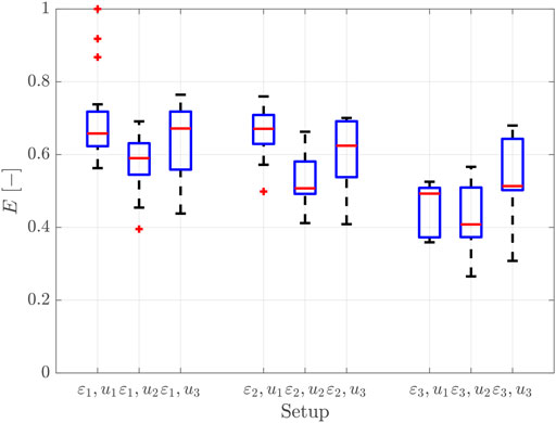
FIGURE 14. Trap efficiency E (-) calculated by Eq. 12 for different investigated fence configurations varying in fence porosity ε₁ = 22.6%, ε₂ = 41.6%, and ε₃ = 56.5% for investigated wind velocities u₁ = 6.1 m/s, u₂ = 7.4 m/s, and u₃ = 9.3 m/s over the whole measuring time t = 600 s.

Generally, the trap efficiency for the dense and medium fence are higher than for the lowest porosity fence. However, the shape of the resulting sediment accretion differs for the fences. Sand-trapping fences with lower porosities (ε₁ = 22.6% and ε₂ = 41.6%) favor localized sediment accretion directly at their brushwood lines. Fences with higher porosity (ε₃ = 56.5%), allow for more sediment accretion further downwind, see also Figure 10. Thus, denser fence porosities are more suitable for constructing sand-trapping fences to initiate and facilitate the coastal dune toe growth. Fences with higher porosity could be used where the sediment accretion would occur over a longer downwind distance, for example, to allow a smoother transition between the foredunes and the white dunes.

Moreover, for the same porosity, the low wind velocity (u₁ = 6.1 m/s) always gives the highest trap efficiency, followed by efficiency for the highest wind velocity (u₃ = 9.3 m/s) and the medium wind velocity (u₂ = 7.4 m/s). This can be explained by the fact that the critical shear stress velocity is minimally exceeded at the lowest wind velocity.

We strongly recommend extending the wind tunnel experiments over longer test sections to gain more quantitative data. This would require much larger wind tunnel dimensions with a larger sediment bed as well as a continuous sediment supply. With these proposed boundaries, it could be measured over more extended periods. Furthermore, installing numerous rows of fences in a larger wind tunnel would allow us to evaluate the optimal distance between numerous rows of fences to favor sediment accretion.

Conclusion

Physical model tests were conducted on sand-trapping fences with different fence heights (h = 40, 80, and 120 mm) and fence porosities (ε = 22.6, 41.6, and 56.5%). These tests occurred in an indoor subsonic, blowing-sand wind tunnel equipped with a moveable sediment bed (d₅₀ ∼ 212 µm). The experimental mean wind velocities were u₁ = 6.1 m/s, u₂ = 7.4 m/s, and u₃ = 9.3 m/s. We used a hot-wire anemometer to measure the flow fields, a vertical mesh sand trap to determine the sediment fluxes, and a 2D laser scanner to record the sediment accretion around the sand-trapping fences over time. The results of these experiments gave the following conclusions:

1) The wind profiles could be measured well with the hot-wire anemometer and provide reproducible data in repeated experiments. We recognized that the wind reduction coefficients varied significantly for different fence porosities and fence heights. It becomes clear that for the medium and high fence, the influence of the porosity is more significant than for the low fence height. However, the fence height plays a minor role for the high fence porosity. For the lower fence porosities, ε₁ = 22.6% and ε₂ = 41.6%, the typical airflow conditions around a single porous fence could be identified. The airflow zones around the fence of porosity ε₃ = 56.5% are less complex.

2) The two-dimensional development of the sediment accretion around the sand-trapping fences could be measured well with the 2D LiDAR scanner and is quantitatively reproducible in repeated experiments. However, for the quantitative evaluation, low wind velocities and high fence porosities associated with low sediment accretion significantly influence the trapping efficiency, where the ratio of the measurement error to the deposition heights is small.

3) For the first time, the influence of model effects in wind tunnel experiments on the sediment accretion around a fence is considered. For this purpose, the different sediment fluxes are differentiated so that the sand-trapping efficiency is specified to the close range of the fence.

4) At the beginning of the experiments, the trap efficiency increases until its maximum, and as time passes, the efficiency decreases slightly or stagnates over an equilibrium during the time investigated in our experiments.

5) The porosity of the fence significantly controls the efficiency to trap sediment. More sediment deposits for fences with porosities of ε₁ = 22.6% and ε₂ = 41.6%, where localized sediment accretion directly at the sand-trapping fence takes place. Fences with higher porosity (ε₃ = 56.5%) and an associated stronger bleed flow, allow for sediment accretion further downwind.

6) We recommend coastal managers to choose the fence porosity depending on the installation purpose. Lower fence porosities can be used to initiate and facilitate the dune toe growth, whereas fences with higher porosity would be more suitable to favor the sediment accretion between the transition of foredunes and white dunes as they have a wider range in which sediment accretes downwind.

The study results are of considerable significance for guidelines on installing sand-trapping fences and can provide theoretical support for their design.

Since experimental time, wind velocity, fence height, and the number of fence rows in wind tunnel investigations are often limited by the dimensions of the wind tunnel, long-term in situ measurements of sediment accretion around sand-trapping fences are needed containing data of changes in topography, beach slope, wet and dry beach width, tidal range, wind direction, and wind velocity.

Data Availability Statement

The raw data supporting the conclusion of this article will be made available by the authors, without undue reservation.

Author Contributions

Conceptualization: CE; methodology: CE; formal analysis: CE; investigation: CE; data processing: CE; resources: HS; original draft preparation: CE; review and editing: HS; visualization: CE; supervision: HS; project administration: HS; and funding acquisition: CE, HS and others. All authors have read and agreed to the published version of the manuscript.

Funding

This research was funded by the German Federal Ministry of Education and Research (BMBF) within the project ProDune (Grant Number 03KIS125) that was initiated in the framework of the German Coastal Engineering Research Council (KFKI).

Conflict of Interest

The authors declare that the research was conducted in the absence of any commercial or financial relationships that could be construed as a potential conflict of interest.

Publisher’s Note

All claims expressed in this article are solely those of the authors and do not necessarily represent those of their affiliated organizations, or those of the publisher, the editors, and the reviewers. Any product that may be evaluated in this article, or claim that may be made by its manufacturer, is not guaranteed or endorsed by the publisher.

Acknowledgments

The authors thank the project partner Lower Saxony Water Management, Coastal Protection and Nature Conservation Agency for sharing their expertise in the project support group. The authors also thank Holger Blum for organizing sediments from the East Frisian Island of Norderney. We, furthermore, thank the technical staff and student assistants Sonja Möller, Mariana Vélez Perez, Marie Künzel, Michael Nelles, and Andrea Limberg of the IWW for their help in constructing and conducting the wind tunnel experiments.

References

Adriani, M. J., and Terwindt, J. (1974). Sand Stabilization and Dune Building. Gov. Publ. off; Government Publ. Office, GBV Gemeinsamer Bibliotheksverbund, the Hague, 68. The Hague: Rijkswaterstaat Communications.

Google Scholar

Anderson, J. D. (2017). Fundamentals of Aerodynamics. McGraw-Hill series in aeronautical and aerospace engineering, 1130.

Google Scholar

Arens, S. M., Baas, A. C. W., Van Boxel, J. H., and Kalkman, C. (2001). Influence of Reed Stem Density on Foredune Development. Earth Surf. Process. Landforms 26, 1161–1176. doi:10.1002/esp.257

CrossRef Full Text | Google Scholar

Baas, A. C. W., and Sherman, D. J. (2006). Spatiotemporal Variability of Aeolian Sand Transport in a Coastal Dune Environment. J. Coastal Res. 225, 1198–1205. doi:10.2112/06-0002.1

CrossRef Full Text | Google Scholar

Bagnold, R. A. (1971). The Physics of Blown Sand and Desert Dunes. 2nd Edition. doi:10.1007/978-94-009-5682-7

CrossRef Full Text | Google Scholar

Barlow, J., William, H., and Pope, A. (1999). Low-Speed Wind Tunnel Testing.

Google Scholar

Bauer, B. O., and Davidson-Arnott, R. G. D. (2003). A General Framework for Modeling Sediment Supply to Coastal Dunes Including Wind Angle, beach Geometry, and Fetch Effects. Geomorphology 49, 89–108. doi:10.1016/S0169-555X(02)00165-4

CrossRef Full Text | Google Scholar

Bauer, B. O., and Davidson-Arnott, R. G. D. (2014). Aeolian Particle Flux Profiles and Transport Unsteadiness. J. Geophys. Res. Earth Surf. 119, 1542–1563. doi:10.1002/2014JF003128

CrossRef Full Text | Google Scholar

Cattafesta, L., Bahr, C., and Mathew, J. (2010). Fundamentals of Wind-Tunnel Design. Encyclopedia Aerospace Eng. 58, 467. doi:10.1002/9780470686652.eae532

CrossRef Full Text | Google Scholar

Cermak, J. E. (1987). Advances in Physical Modeling for Wind Engineering. J. Eng. Mech. 113113, 7375–7756. doi:10.1061/(ASCE)0733-939910.1061/(asce)0733-9399(1987)113:5(737)

CrossRef Full Text | Google Scholar

Chen, B., Cheng, J., Xin, L., and Wang, R. (2019). Effectiveness of Hole Plate-type Sand Barriers in Reducing Aeolian Sediment Flux: Evaluation of Effect of Hole Size. Aeolian Res. 38, 1–12. doi:10.1016/j.aeolia.2019.03.001

CrossRef Full Text | Google Scholar

Cohn, N., Hoonhout, B., Goldstein, E., de Vries, S., Moore, L., Durán Vinent, O., et al. (2019). Exploring Marine and Aeolian Controls on Coastal Foredune Growth Using a Coupled Numerical Model. JMSE 7, 13. doi:10.3390/jmse7010013

CrossRef Full Text | Google Scholar

Cohn, N., Ruggiero, P., Vries, S., and Kaminsky, G. M. (2018). New Insights on Coastal Foredune Growth: The Relative Contributions of Marine and Aeolian Processes. Geophys. Res. Lett. 45, 4965–4973. doi:10.1029/2018GL077836

CrossRef Full Text | Google Scholar

Cornelis, W. M., and Gabriels, D. (2005). Optimal Windbreak Design for Wind-Erosion Control. J. Arid Environments 61, 315–332. doi:10.1016/j.jaridenv.2004.10.005

CrossRef Full Text | Google Scholar

Creyssels, M., Dupont, P., El Moctar, A. O., Valance, A., Cantat, I., Jenkins, J. T., et al. (2009). Saltating Particles in a Turbulent Boundary Layer: experiment and Theory. J. Fluid Mech. 625, 47–74. doi:10.1017/S0022112008005491

CrossRef Full Text | Google Scholar

Davidson-Arnott, R. G. D., MacQuarrie, K., and Aagaard, T. (2005). The Effect of Wind Gusts, Moisture Content and Fetch Length on Sand Transport on a beach. Geomorphology 68, 115–129. doi:10.1016/j.geomorph.2004.04.008

CrossRef Full Text | Google Scholar

de Vries, S. (2013). Physics Of Blown Sand and Coastal Dunes. Dissertation. Delft,Netherlands: Delft University of Technology.

Google Scholar

DIN EN ISO 14688-1 (2018). Geotechnische Erkundung und Untersuchung – Benennung, Beschreibung und Klassifizierung von Boden: Teil 1. Benennung und Beschreibung. doi:10.31030/2748424

CrossRef Full Text | Google Scholar

Dong, Z., Luo, W., Qian, G., and Wang, H. (2007). A Wind Tunnel Simulation of the Mean Velocity fields behind Upright Porous Fences. Agric. For. Meteorology 146, 82–93. doi:10.1016/j.agrformet.2007.05.009

CrossRef Full Text | Google Scholar

Eichmanns, C., Lechthaler, S., Zander, W., Pérez, M. V., Blum, H., Thorenz, F., et al. (2021). Sand Trapping Fences as a Nature-Based Solution for Coastal Protection: An International Review with a Focus on Installations in Germany. Environments 8, 135. doi:10.3390/environments8120135

CrossRef Full Text | Google Scholar

Eichmanns, C., and Schüttrumpf, H. (2021). Influence of Sand Trapping Fences on Dune Toe Growth and its Relation with Potential Aeolian Sediment Transport. JMSE 9, 850. doi:10.3390/jmse9080850

CrossRef Full Text | Google Scholar

Eichmanns, C., and Schüttrumpf, H. (2020). Investigating Changes in Aeolian Sediment Transport at Coastal Dunes and Sand Trapping Fences: A Field Study on the German Coast. JMSE 8, 1012. doi:10.3390/jmse8121012

CrossRef Full Text | Google Scholar

Ellis, J. T., Li, B., Farrell, E. J., and Sherman, D. J. (2009). Protocols for Characterizing Aeolian Mass-Flux Profiles. Aeolian Res. 1, 19–26. doi:10.1016/j.aeolia.2009.02.001

CrossRef Full Text | Google Scholar

Gallego-Fernández, J. B. (2013). Restoration of Coastal Dunes. Berlin, Heidelberg: Springer Berlin/Heidelberg.

Google Scholar

Gerhardt, P. (1990). Handbuch des deutschen Dünenbaus. Berlin.

Google Scholar

Hacker, S. D., Zarnetske, P., Seabloom, E., Ruggiero, P., Mull, J., Gerrity, S., et al. (2012). Subtle Differences in Two Non-native Congeneric beach Grasses Significantly Affect Their Colonization, Spread, and Impact. Oikos 121, 138–148. doi:10.1111/j.1600-0706.2011.18887.x

CrossRef Full Text | Google Scholar

Han, Q., Qu, J., Liao, K., Zhu, S., Zhang, K., Zu, R., et al. (2011). A Wind Tunnel Study of Aeolian Sand Transport on a Wetted Sand Surface Using Sands from Tropical Humid Coastal Southern China. Environ. Earth Sci. 64, 1375–1385. doi:10.1007/s12665-011-0962-7

CrossRef Full Text | Google Scholar

Harff, J., Björck, S., and Hoth, P. (2011). The Baltic Sea basin. Berlin: Springer.

Google Scholar

Hesp, P. (2011). Dune Coasts. Earth Syst. Environ. Esciences, 193–221. doi:10.1016/B978-0-12-374711-2.00310-7

CrossRef Full Text | Google Scholar

Ho, T. D., Dupont, P., Ould El Moctar, A., and Valance, A. (2012). Particle Velocity Distribution in Saltation Transport. Phys. Rev. E 85, 52301. doi:10.1103/PhysRevE.85.052301

PubMed Abstract | CrossRef Full Text | Google Scholar

Ho, T. D., Valance, A., Dupont, P., and Ould El Moctar, A. (2011). Scaling Laws in Aeolian Sand Transport. Phys. Rev. Lett. 106, 94501. doi:10.1103/PhysRevLett.106.094501

CrossRef Full Text | Google Scholar

Hotta, S., and Horikawa, K. (1991). Function of Sand Fence Placed in Front of Embankment. Proc. 22nd Conf. Coastal Eng., 2754–2767. doi:10.1061/9780872627765.211

CrossRef Full Text | Google Scholar

Houser, C., Wernette, P., Rentschlar, E., Jones, H., Hammond, B., and Trimble, S. (2015). Post-storm beach and Dune Recovery: Implications for Barrier Island Resilience. Geomorphology 234, 54–63. doi:10.1016/j.geomorph.2014.12.044

CrossRef Full Text | Google Scholar

Itzkin, M., Moore, L. J., Ruggiero, P., Hacker, S. D., and Biel, R. G. (2020b). The Influence of Dune Aspect Ratio, Beach Width and Storm Characteristics on Dune Erosion for Managed and Unmanaged Beaches.

Google Scholar

Itzkin, M., Moore, L. J., Ruggiero, P., and Hacker, S. D. (2020a). The Effect of Sand Fencing on the Morphology of Natural Dune Systems. Geomorphology 352, 106995. doi:10.1016/j.geomorph.2019.106995

CrossRef Full Text | Google Scholar

Jackson, D. W. T., and Cooper, J. A. C. (1999). Beach Fetch Distance and Aeolian Sediment Transport. Sedimentology 46, 517–522. doi:10.1046/j.1365-3091.1999.00228.x

CrossRef Full Text | Google Scholar

Jackson, N. L., and Nordstrom, K. F. (2011). Aeolian Sediment Transport and Landforms in Managed Coastal Systems: A Review. Aeolian Res. 3, 181–196. doi:10.1016/j.aeolia.2011.03.011

CrossRef Full Text | Google Scholar

Keijsers, J. G. S., De Groot, A. V., and Riksen, M. J. P. M. (2015). Vegetation and Sedimentation on Coastal Foredunes. Geomorphology 228, 723–734. doi:10.1016/j.geomorph.2014.10.027

CrossRef Full Text | Google Scholar

Lawlor, P., and Jackson, D. (2021). “A Nature-Based Solution for Coastal Foredune Restoration: The Case Study of Maghery, County Donegal, Ireland,” in Book: Exploring the Multiple Values of Nature: Connecting Ecosystems and People across Landscapes. 1st Edition (Springer Nature).

Google Scholar

Lee, S.-J., and Kim, H.-B. (1999). Laboratory Measurements of Velocity and Turbulence Field behind Porous Fences. J. Wind Eng. Ind. Aerodynamics 80, 311–326. doi:10.1016/S0167-6105(98)00193-7

CrossRef Full Text | Google Scholar

Li, B., and Sherman, D. J. (2015). Aerodynamics and Morphodynamics of Sand Fences: A Review. Aeolian Res. 17, 33–48. doi:10.1016/j.aeolia.2014.11.005

CrossRef Full Text | Google Scholar

Manohar, M., and Bruun, P. (1970). Mechanics of Dune Growth by Sand Fences. Dock and harbour authority, 243–252.

Google Scholar

MATLAB (2018). Natick, Massachusetts: The MathWorks Inc. Version 9.510.944444 (R2018b)Available at: https://de.mathworks.com/products/new_products/release2018b.html (Accessed March 31, 2021).

Mehta, R. D. (1979). The Aerodynamic Design of Blower Tunnels with Wide-Angle Diffusers. Prog. Aerospace Sci. 18, 59–120. doi:10.1016/0376-0421(77)90003-3

CrossRef Full Text | Google Scholar

Miri, A., Dragovich, D., and Dong, Z. (2019). Wind-borne Sand Mass Flux in Vegetated Surfaces - Wind Tunnel Experiments with Live Plants. CATENA 172, 421–434. doi:10.1016/j.catena.2018.09.006

CrossRef Full Text | Google Scholar

Mulhearn, P. J., and Bradley, E. F. (1977). Secondary Flows in the lee of Porous Shelterbelts.

Google Scholar

NASA (2020). Living Ocean.

Google Scholar

Nickling, W. G., and Davidson-Arnott, R. G. D. (1990). Aeolian Sediment Transport on Beaches and Coastal Sand Dunes. Proceedings Canadian Symposium on Costal Sand Dunes 1990. Proc. Symp. Coastal Sand Dunes, 1–36.

Google Scholar

Nikuradse, J. (1933). Strömungsgesetze in Rauhen Rohren. English: Flow laws in rough pipes.

Google Scholar

Ning, Q., Li, B., and Ellis, J. T. (2020). Fence Height Control on Sand Trapping. Aeolian Res. 46, 100617. doi:10.1016/j.aeolia.2020.100617

CrossRef Full Text | Google Scholar

O'Connel, J. (2008). Coastal Dune Protection & Restoration: Using ‘Cape’ American Beach Grass And Fencing.

Owen, P. R., and Gillette, D. (1985). “Wind Tunnel Constraint on Saltati,” in Proceedings of the International Workshop on the Physics of Blown Sand, 253–269.

Google Scholar

Perera, M. D. A. E. S. (1981). Shelter behind Two-Dimensional Solid and Porous Fences. J. Wind Eng. Ind. Aerodynamics 8, 93–104. doi:10.1016/0167-6105(81)90010-6

CrossRef Full Text | Google Scholar

Plate, E. J. (1971). The Aerodynamics of Shelter Belts. Agric. Meteorology 8, 203–222. doi:10.1016/0002-1571(71)90109-9

CrossRef Full Text | Google Scholar

Poortinga, A., Keijsers, J. G. S., Maroulis, J., and Visser, S. M. (2014). Measurement Uncertainties in Quantifying Aeolian Mass Flux: Evidence from Wind Tunnel and Field Site Data. PeerJ 2, e454. doi:10.7717/peerj.454

PubMed Abstract | CrossRef Full Text | Google Scholar

Ruz, M.-H., and Anthony, E. J. (2008). Sand Trapping by Brushwood Fences on a beach-foredune Contact: the Primacy of the Local Sediment Budget. zfg_suppl 52, 179–194. doi:10.1127/0372-8854/2008/0052S3-0179

CrossRef Full Text | Google Scholar

Shao, Y., and Lu, H. (2000). A Simple Expression for Wind Erosion Threshold Friction Velocity. J. Geophys. Res. 105, 22437–22443. doi:10.1029/2000JD900304

CrossRef Full Text | Google Scholar

Sherman, D. J., Swann, C., and Barron, J. D. (2014). A High-Efficiency, Low-Cost Aeolian Sand Trap. Aeolian Res. 13, 31–34. doi:10.1016/j.aeolia.2014.02.006

CrossRef Full Text | Google Scholar

Strypsteen, G. (2019). Monitoring and Modelling Aeolian Sand Transport at the Belgian Coast. Leuven, Belgium: Dissertation. KU Leuven, Faculty of Engineering Technology, 1–226. doi:10.13140/RG.2.2.19781.88806

CrossRef Full Text | Google Scholar

Swann, C., Brodie, K., and Spore, N. (2015). Coastal Foredunes: Identifying Coastal, Aeolian, and Management Interactions Driving Morphologic State Change: ERDC/CHL TR-15-17. Washington, DC 20314: U.S. Army Corps of Engineers–1000.

Google Scholar

testo (2021). Hot-wire Anemometer and External Data Logger: Product Specifications. Testo SE & Co. KGaA.

Google Scholar

van Rijn, L. C. (2019). Aeolian Transport over a Flat Sediment Surface.

Google Scholar

van Rijn, L. C., and Strypsteen, G. (2020). A Fully Predictive Model for Aeolian Sand Transport. Coastal Eng. 156, 103600. doi:10.1016/j.coastaleng.2019.103600

CrossRef Full Text | Google Scholar

van Thiel de Vries, J. S. M. (2009). Dune Erosion during Storm Surges. Dissertation. Netherlands. Amsterdam: Delft University of Technology, Civil Engineering and Geosciences, Hydraulic EngineeringTechnische Universität Delft.

Google Scholar

Vithana, (2013). The Effect of Stone Protrusion on the Incipient Motion of Rock armour under the Action of Regular Waves. London: Department of Civil, Environmental & Geomatic Engineering, University College London.

Google Scholar

Wang, T., Qu, J., Ling, Y., Liu, B., and Xiao, J. (2018). Shelter Effect Efficacy of Sand Fences: A Comparison of Systems in a Wind Tunnel. Aeolian Res. 30, 32–40. doi:10.1016/j.aeolia.2017.11.004

CrossRef Full Text | Google Scholar

White, R. R. (1996). Laboratory Simulation of Aeolian Sand Transport and Physical Modeling of Flow Around Dunes. Annals of Arid Zone, 187–213.

Google Scholar

Yu, Y.-p., Zhang, K.-c., An, Z.-s., Wang, T., and Hu, F. (2020). The Blocking Effect of the Sand Fences Quantified Using Wind Tunnel Simulations. J. Mt. Sci. 17, 2485–2496. doi:10.1007/s11629-020-6095-2

CrossRef Full Text | Google Scholar

Zhang, N., Kang, J.-H., and Lee, S.-J. (2010). Wind Tunnel Observation on the Effect of a Porous Wind Fence on Shelter of Saltating Sand Particles. Geomorphology 120, 224–232. doi:10.1016/j.geomorph.2010.03.032

CrossRef Full Text | Google Scholar