Probabilistic Multi-Objective Inverse Analysis for Damage Identification Using Piezoelectric Impedance Measurement Under Uncertainties

1 Introduction

Structural health monitoring (SHM) has been an important research subject, as it can provide vital information to protect engineering structures from unexpected catastrophic failure. A wide variety of investigations have utilized vibration measurement to conduct SHM tasks. The modal properties such as natural frequencies and mode shapes extracted from the vibration measurement can be used effectively to predict the structural property change due to damage (Cao et al., 2014; Capecchi et al., 2016). However, in actual practice, only lower-order modes can be realistically measured, which, however, are insensitive to small-sized damage. In order to detect and identify small-sized damage, high-frequency measurements with small characteristic wavelengths need to be acquired. One promising class of high-frequency-based detection methods is to use piezoelectric transducers which can yield the impedance or admittance information through active interrogation to facilitate fault detection and identification (Kim et al., 2015; Shuai et al., 2017; Cao et al., 2018; Kim and Wang, 2019). Impedance/admittance-based methods for damage identification rely on inherent electro-mechanical coupling. When a piezoelectric transducer is attached to a host structure, the electrical impedance of the transducer is directly coupled with the impedance of the host structure. As such, the change of the piezoelectric impedance signature can be used as the damage indicator. Owing to the self-sensing interrogative nature whereas the transducers serve as both the actuators and sensors, these methods enable highly sensitive damage detection.

Conducting damage identification generally resorts to the comparison of responses before and after damage occurrence. Leveraging upon finite element (FE) simulation to map the relation between the damage and resulting impedance/admittance response change, damage identification can then be facilitated. This approach falls into the general category of FE model updating which has become the mainstream for damage identification analysis (Zhou and Tang, 2016; Sun et al., 2017; Chen et al., 2020; Zhou and Tang, 2021b). In this approach, the damage is represented by the change of the associated structural properties, for example, mass, stiffness, and damping, and can be inversely identified in light of the measurements. Since it is critical to accurately capture the small change of impedance/admittance response due to damage, the element size should be set very small, resulting in a high-dimensional FE model. It generally leads to high computational costs in model updating. To tackle this issue, a variety of efficient approximators have been explored. Along with the recent development of machine learning technology, surrogate models have been recognized as one effective type of approximator. Once the surrogate model is trained by the credible input–output relations from FE simulations, it can be directly utilized to approximate the output given any input (Khodaparast et al., 2011; Wan and Ren, 2015; Zhou and Tang, 2021a). A noteworthy challenge of the surrogate model-based inverse analysis is its lack of ability to handle noise and uncertainty effects. Moreover, in such data-driven methods, the size and distribution of training data play an important role in dictating damage identification accuracy. The high-fidelity surrogate model may not be ensured over the entire input parametric space, which may cause prediction errors that even exceed the response changes induced by damage. The first-principle-based approximator, on the other hand, may possess higher approximation accuracy than the surrogate model. As one class of first-principle-based approximation methods, sensitivity analysis has been extensively applied (Mottershead et al., 2011; Zhou and Tang, 2015; Shuai et al., 2017; Zhu et al., 2021). The underlying idea of the sensitivity analysis is to calculate the sensitivity matrices based on the FE model using the finite difference concept, which can then be used for rapid response approximation.

Fundamentally, inverse model/damage identification can be cast into an optimization problem that aims at minimizing the difference between the measurements and model prediction in the parametric space. The aforementioned sensitivity-based approach can be viewed as a special treatment for solving such optimization problems. Oftentimes, a single objective function, that is, a holistic error function between the measurement and model prediction, is minimized. In the case of damage identification using piezoelectric impedance/admittance, such a single-objective approach becomes difficult to implement. On the one hand, to predict high-frequency impedance/admittance responses, the mesh density of the FE model has to be high, yielding a very large number of unknowns because the structural damage can occur in an arbitrary region with arbitrary severity in the model. On the other hand, the impedance/admittance measurements remain to be relatively limited. As the number of unknowns is far greater than the available measurement data points, the direct inverse analysis becomes underdetermined. Meanwhile, a single objective optimization generally leads to one single solution. As such, the solution found may not cover the actual damage scenario (Cao et al., 2018).

In comparison, multi-objective optimization can intrinsically yield multiple solutions and thus has much better possibility of capturing the actual damage scenario. Indeed, since multiple measurements are acquired in SHM practice, formulating the multi-objective optimization problem that minimizes the difference of these measurements with respect to the corresponding model prediction in the parametric space is quite intuitive. The multiple solutions obtained can then be further analyzed either through empirical experience or by deploying the additional inspection techniques. Owing to these advantages, some recent investigations have attempted multi-objective optimization in damage identification. Cao et al. (2018) proposed a multi-objective Dividing RECTangles (DIRECT) under embedded sparsity conditions to perform damage identification using the piezoelectric impedance/admittance measurement. Alexandrino et al. (2020) developed a robust framework integrating together a multi-objective genetic algorithm, neural network, and decision-making strategy to solve the damage detection problem. Magacho et al. (2021) used the multi-objective sunflower optimization algorithm to identify the damage in large-scale lattice-type structures. It is, however, worth emphasizing that the aforementioned studies were conducted on the premise that the experimental measurement and numerical FE model are both sufficiently accurate. In practical situations, both the measurement and numerical modeling are inevitably subjected to noise and uncertainties. To tackle this issue, in this research, we propose to develop a new multi-objective optimization approach that can produce solutions in the probabilistic sense to reflect the influence of noise and uncertainty. The key idea is to use statistical methodologies for characterizing sampled solutions that are uniformly scattered around the Pareto optimal set (Zhang et al., 2008). This is realized through integrating the differential evolution MCMC algorithm into the multi-objective optimization framework.

The remainder of this study is organized as follows: Section 2 outlines the new damage identification framework, including the FE-based piezoelectric impedance/admittance modeling and probabilistic multi-objective MCMC optimization. Section 3 provides the case illustrations with experimental investigation. Section 4 summarizes the concluding remarks.

2 Approach Formulation for Damage Identification

2.1 Admittance Measurement-Based Damage Identification Using Sensitivity Concept

The equation of motion of the coupled system consisting of the host structure and piezoelectric transducer with an electric circuit can be written as (Zhou et al., 2014):

$\mathbf{M}\ddot{\mathbf{q}}+\mathbf{C}\dot{\mathbf{q}}+\mathbf{Kq}+{\mathbf{K}}_{\mathbf{12}}Q=\mathbf{0,}(1)$

$K_{c}Q+{\mathbf{K}}_{12}^T\mathbf{q}+R\dot{Q}=V_{in},(2)$

where $\mathbf{q}$ is the displacement vector. M, K, and C are the mass, stiffness, and damping matrices of the host structure, respectively. ${\mathbf{K}}_{12}$ is the coupling vector, $K_c$ is the inverse of the capacitance of the piezoelectric transducer, R is the resistance of the electric circuit, $Q$ is the electrical charge on the surface of the piezoelectric transducer, and $V_{in}$ is the input voltage. As the frequency sweeping of the input voltage is applied, Eqs 1, 2 can be transferred to the frequency domain, and the admittance of the piezoelectric transducer can be obtained as follows (note: the admittance here is the reciprocal of the impedance) (Wang and Tang, 2009):

$Y\left(\omega \right)=\frac{\dot{Q}}{V_{in}}=\frac{j\omega }{j\omega R+K_c-{\mathbf{K}}_{12}^T\left(\mathbf{K}+j\omega \mathbf{C}-{\omega }^2\mathbf{M}\right){\mathbf{K}}_{12}},(3)$

where $\omega$ is the angular frequency and j is the imaginary unit. Eq. 3 indicates that the admittance of the piezoelectric transducer is coupled with the mechanical properties of the host structure. Structural damage is commonly assumed as localized changes in structural stiffness. Then, structural property changes induced by damage will be reflected in the changes of admittance of the piezoelectric transducer, given as:

$Y_d\left(\omega \right)=\frac{{\dot{Q}}_d}{V_{in}}=\frac{j\omega }{j\omega R+K_c-{\mathbf{K}}_{12}^T\left({\mathbf{K}}_d+j\omega \mathbf{C}-{\omega }^2\mathbf{M}\right){\mathbf{K}}_{12}},(4)$

where ${\mathbf{K}}_d$ is the stiffness matrix of the damaged structure (Xia and Hao, 2003).

${\mathbf{K}}_d={\displaystyle \sum _{j=1}^m{\mathbf{K}}_{hj}\left(1-{\alpha }_j\right)}.(5)$

In Eq. 5, ${\mathbf{K}}_{hj}$ is the stiffness sub-matrix of the jth segment of a healthy structure, $m$ indicates the number of segments susceptible to damage occurrence in the structure, and ${\alpha }_j\in \left[\mathrm{0,1}\right]$ is the damage index which indicates the stiffness loss of the jth segment. For example, if the jth element suffers from damage that leads to a 10% of stiffness loss, then ${\alpha }_j=0.1$. In the damage identification analysis, the measured admittance of the damaged structure needs to be compared with that of the healthy structure.

According to Eqs 4, 5, the admittance changes are not linearly dependent with respect to the damage index. In order to approximate the linear relationship between the admittance changes and damage index under the small damage assumption, a Taylor series expansion is applied and only the linear terms are kept:

$Y_d\left(\mathbf{\alpha }\right)\approx Y\left(\mathbf{\alpha }=\mathrm{0}\right)+{\displaystyle \sum _{j=1}^m\frac{\partial Y}{\partial {\alpha }_j}}{|}_{{\alpha }_j=0}{\alpha }_j,(6)$

where

$\frac{\partial Y}{\partial {\alpha }_j}{|}_{{\alpha }_j=0}=\omega \text{i}{\left[k_c-{\mathbf{K}}_{12}^T({\mathbf{K}-\mathbf{M}{\omega }^2+\mathbf{C}\omega \text{i})}^{-}{\mathbf{K}}_{12}\right]}^{-2}{\mathbf{K}}_{12}^T\left[\frac{\partial {\left({\mathbf{K}}_d-\mathbf{M}{\omega }^2+\mathbf{C}\omega \mathrm{i}\right)}^{-}}{\partial {\alpha }_j}{|}_{{\alpha }_j=0}\right]{\mathbf{K}}_{12}.(7)$

The admittance changes can then be written as a linear function of the damage index ${\alpha }_j$:

$\mathrm{\Delta }Y\left(\omega \right)=Y_d-Y\left(\mathbf{\alpha }\mathrm{=0}\right)={\displaystyle \sum _{j=1}^m\left[\omega \text{i}{\left(k_c-{\mathbf{K}}_{12}^T{\mathbf{Z}}^{-}{\mathbf{K}}_{12}\right)}^{-2}{\mathbf{K}}_{12}^T{\mathbf{Z}}^{-}\left({\mathbf{L}}_j^T{\mathbf{K}}_{ej}{\mathbf{L}}_j\right){\mathbf{Z}}^{-}{\mathbf{K}}_{12}\right]}{\alpha }_j,(8)$

$\mathbf{Z}=\mathbf{K}-\mathbf{M}{\omega }^2+\text{i}\omega \mathbf{C,}(9)$

where $\mathbf{Z}$ denotes the dynamic stiffness of the structure and $\mathbf{L}$ indicates how the elemental matrices are assembled into the global stiffness matrix. Eq. 8 exhibits the relationship between the admittance changes and damage index at a single excitation frequency point $\omega$. Theoretically, such a relationship holds at every frequency point. Then, if admittances are measured at q points, q equations will be formulated to establish the relation as a matrix form,

$\mathrm{\Delta }{\mathbf{Y}}_{q\times 1}=\left[\begin{array}{c}\mathrm{\Delta }Y\left({\omega }_1\right)\\ ⋮\\ \mathrm{\Delta }Y\left({\omega }_q\right)\end{array}\right]={\mathbf{S}}_{q\times m}{\mathbf{\alpha }}_{m\times 1},(10)$

where $\Delta {\mathbf{Y}}_{q\times 1}$ is the admittance changes observed at m frequency points, ${\mathbf{\alpha }}_{m\times 1}$ is the vector of m unknown damage indices, and ${\mathbf{S}}_{q\times m}$ is the sensitivity matrix. The direct inversion of the matrix ${\mathbf{S}}_{q\times m}$ may lead to the numerical issue when the sensitivity matrix ${\mathbf{S}}_{q\times m}$ is ill-conditioned. To avoid the matrix inversion, we only use such sensitivity-based relation as an efficient approximator to predict the admittance response in the parametric space when carrying out the damage identification analysis.

2.1.1 Multi-Objective Markov Chain Monte Carlo for Probabilistic Optimization

Let a continuous multi-objective optimization problem be defined as

$\begin{array}{l}\min \left(\mathbf{f}\left(\mathbf{x}\right)\right)\mathbf{f}\left(\mathbf{x}\right)=\left[f_1\left(\mathbf{x}\right),f_2\left(\mathbf{x}\right),\dots f_n\left(\mathbf{x}\right)\right],\\ \text{subject}\text{to}\mathbf{x}\in \mathbf{X}\subset {\text{R}}^m,\end{array}(11)$

where x denotes the m-dimensional decision vector and $\mathbf{f}\left(\mathbf{x}\right)$ denotes the n-dimensional vector of objective functions. In this research, x is the vector of damage index variables (i.e., ${\mathbf{\alpha }}_{m\times 1}$ in Eq. 10), whereas the admittance response changes over different excitation frequencies altogether constitute the vector of objective functions $\mathbf{f}\left(\mathbf{x}\right)$.

Solving the multi-objective optimization shown in Eq. 11 yields a set of trade-off solutions referred to as the Pareto optimal set, which represents the decision vector solutions whose respective objective functions cannot be enhanced in any direction without degrading the other (Zitzler and Thiele, 1999). The Pareto optimal set usually can be determined by evaluating the dominance relations among a set of solutions. A solution ${\mathbf{x}}_{\mathit{i}}$ that dominates another solution ${\mathbf{x}}_j$ is described as ${\mathbf{x}}_i\prec {\mathbf{x}}_j$, which holds only if

$\forall r\in \left\{\mathrm{1,2},\dots ,n\right\}:f_r\left({\mathbf{x}}_i\right)\le f_r\left({\mathbf{x}}_j\right).(12)$

It is worth noting that most of the existing algorithms have been designed to target the Pareto optimal set deterministically. When uncertainties are involved, the probabilistic approach will need to be adopted to yield the Pareto optimal set that is represented in a probabilistic sense. The underlying idea behind such a probabilistic approach is to use statistical methodologies for characterizing sampled solutions that are uniformly scattered around the Pareto optimal set (Zhang et al., 2008). Specifically, we seek solutions in the vicinity of the Pareto optimal set such that the uncertainty effect can be characterized for every dominant solution within the Pareto optimal set. To achieve this, we construct a probability distribution using the MCMC algorithm, which is expressed as (Kirkpatrick et al., 1983):

$\pi \left(\mathbf{x}\right)\propto \exp \left(\frac{-\eta \left(\mathbf{x}\right)}{T}\right)T>0,(13)$

where T is the simulated temperature. $\eta \left(\mathbf{x}\right)$ is the fitness function, which is dependent on the objective functions $\mathbf{f}\left(\mathbf{x}\right)$ to be defined subsequently. Since MCMC aims to sample the solutions in the vicinity of the global optimum in order to approximate $\pi \left(\mathbf{x}\right)$, MCMC can be used for optimization purposes.

While the aforementioned MCMC-based optimization concept has already been established, it is generally tailored for the single-objective optimization problem. To extend it into the multi-objective optimization, we specifically need to integrate differential evolution (DE) into the MCMC to form the so-called differential evolution Markov chain Monte Carlo (DEMC) that was originally proposed by Braak (2006). DEMC is a special type of population-based multi-objective Markov chain Monte Carlo (MOMCMC). DEMC involves the multiple Markov chains in parallel to generate new solutions over an entire parameter space based on the current solution. In this approach, a new solution proposal at the tth state of the kth Markov chain is formulated as the sum of its current state and the scaled difference between the current states of two randomly selected chains, given as:

${\mathbf{x}}_k^{t+1}={\mathbf{x}}_k^t+\gamma \left({\mathbf{x}}_a^t-{\mathbf{x}}_b^t\right),(14)$

where ${\mathbf{x}}_k^{t+1}$ and ${\mathbf{x}}_k^t$ represent the current and proposed new solutions, respectively, of the kth Markov chain. ${\mathbf{x}}_a^t$ and ${\mathbf{x}}_b^t$ denote the current solutions of two randomly chosen Markov chains. Subscripts a and b are two random integers from the interval [0, M], where M is the population size or the number of Markov chains. $\gamma$ is a scaled factor, the suggested value of which can be determined using $2.38/\sqrt{\left(2m\right)}$ (Braak, 2006). One may notice that Eq. 14 fundamentally points to the crossover operation in the genetic algorithm (GA) because DE is a GA-based global optimization method (Storn and Price, 1997). The DE-based solution proposal function (Eq. 14) takes advantage of the distance and direction information contained in the current solutions, leading to the fast MCMC convergence.

When carrying out the DEMC-based sampling to achieve the multi-objective function optimization, special care should be taken in defining the fitness function. While it is seemingly straightforward to use the objective function as the fitness function, its resulting solutions may not be sufficiently diverse. In other words, the solutions may be clustered, and near-Pareto optimal solutions that account for the uncertainty effect will be missing. Therefore, a new fitness function of the individual solution suggested by Li (2012) is defined as:

$\eta \left({\mathbf{x}}_i\right)=\{\begin{array}{cc}c\left({\mathbf{x}}_i\right),& {\mathbf{x}}_i\text{is}\text{non}-\text{dominated,}\\ 1+{\displaystyle \sum _j^{{\mathbf{x}}_j\prec {\mathbf{x}}_i}\text{HYP}\left({\mathbf{x}}_i,{\mathbf{x}}_j\right),}& {\mathbf{x}}_i\text{is}\text{dominated,}\end{array}(15)$

where $c\left({\mathbf{x}}_i\right)$ is defined as the proportion of total solutions dominated by ${\mathbf{x}}_i$. HYP is the pair-wise hypervolume surrounded by two solutions ${\mathbf{x}}_i$ and ${\mathbf{x}}_j$ that is used to estimate the significance of dominance. For demonstration, the pair-wise hypervolume of the bi-objective optimization is shown in Figure 1. The pair-wise hypervolume generically can be calculated using the Lebesgue measure (Bartle, 1995) regardless of the objective function dimension. With this new fitness function, the favorability of two solutions can be more easily discriminated, which as a result increases the solution diversity.

FIGURE 1

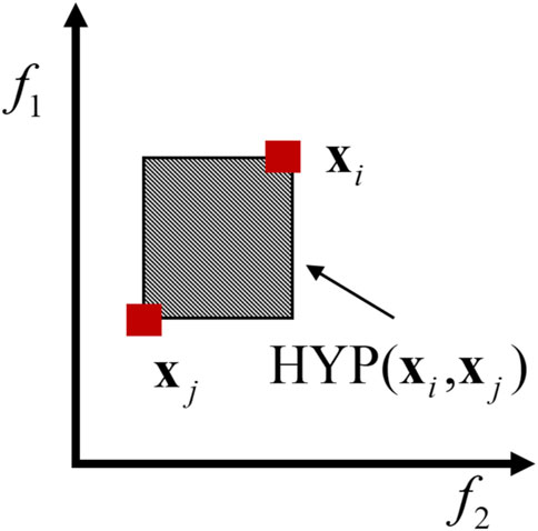
FIGURE 1. Illustration of hypervolume in the bi-optimization problem.

The Metropolis–Hasting (MH) algorithm (Brooks et al., 2011; Zhou and Tang, 2021) is used to determine if the new solution proposed by DE is accepted which recalls Eq. 13. The acceptance probability can then be formulated as:

$p\left({\mathbf{x}}_k^{t+1}|{\mathbf{x}}_k^t\right)=\min \left(1,\frac{\pi \left({\mathbf{x}}_k^{t+1}\right)}{\pi \left({\mathbf{x}}_k^t\right)}\right)=\min \left(1,\exp \left(\frac{-\left(\eta \left({\mathbf{x}}_k^{t+1}\right)-\eta \left({\mathbf{x}}_k^t\right)\right)}{T}\right)\right).(16)$

It can be clearly seen that the simulated temperature controls the acceptance rate of the MH transitions. The acceptance rate of each iteration can be calculated, which together with the desired acceptance rate specified, determines the new temperature for the next iteration. When the MOMCMC is executed, its convergence is worth examining considering the trade-off between the computational cost and accuracy. Generally, both the standard convergence indicator and the maximum iteration number defined can be used as a termination criterion. For the sake of implementation, in this research, we terminate the analysis when the maximum iteration number is reached and then use the analysis result to examine the convergence.

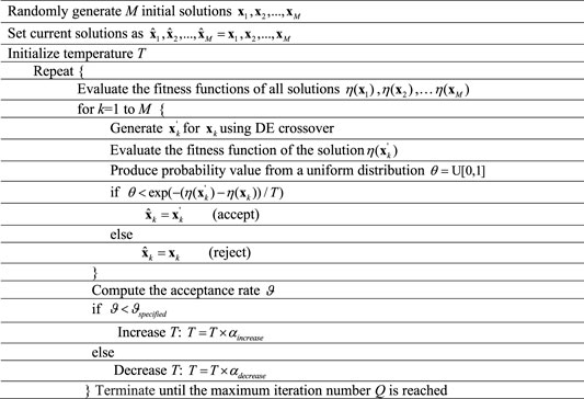
Combining all the above-mentioned steps, we can obtain the pseudo-code of MOMCMC for probabilistic optimization as follows:

3 Methodology Demonstration and Case Analysis

In this section, we demonstrate the new methodology through case illustrations. To fully verify the effectiveness of this new methodology, we formulate the two testing cases, both of which are validated through experimental investigations.

3.1 Problem Setup of Case Investigation

The structure to be investigated is a cantilever aluminum plate that is attached to a piezoelectric transducer. The material and geometrical properties of the plate and piezoelectric transducer are given in Table 1, and the experiment setup is shown in Figure 2. A resistor of 100 $\Omega$ is connected in series with the piezoelectric transducer to measure the voltage drop (Figure 2). A signal analyzer (Agilent 35670A) with a source channel is used. The source channel is used to generate sinusoidal voltage sent to the piezoelectric transducer $\left(V_{in}\right)$, and the output voltage across the resistor is recorded $\left(V_{out}\right)$. Hence, the admittance can be computed as:

$Y_{\exp }=\frac{I}{V_{in}}=\frac{V_{out}}{R_s{V}_{in}}.(17)$

TABLE 1

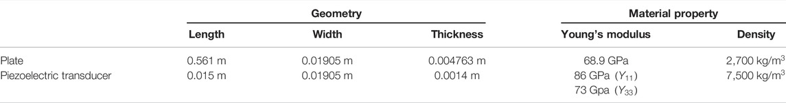
TABLE 1. Geometrical and material properties of the plate and piezoelectric transducer.

FIGURE 2

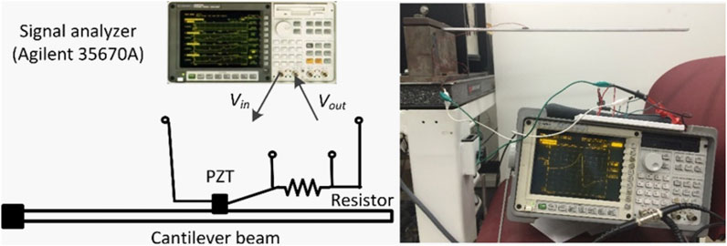
FIGURE 2. Experimental setup.

In the model updating-based damage identification, an electromechanical FE model accounting for the coupling between the plate and piezoelectric transducer is developed using the in-house MATLAB finite element code. The material and geometrical properties in Table 1 are used to build the FE model. In addition, in the FE model, the piezoelectric and impermittivity constants of the piezoelectric transducer are defined as $h_{31}=-1.0288\times {10}^9{\text{Vm}}^{-1}$ and ${\beta }_{33}=1.3832\times {10}^8{\text{mF}}^{-1}$, respectively. The 20-node hexahedron element is used, and the entire FE model consists of 11,250 elements in total. Prior to damage identification, we need to calibrate the FE model of the healthy structure to match the experiment setup because the FE model error usually is induced by non-perfect boundary conditions. Therefore, in this research, we update the boundary conditions to minimize the discrepancy between the actual measurements and model predictions. As indicated in the previous research (Shuai et al., 2017), this is an important step to ensure the subsequent investigation of damage identification.

For damage identification illustration, the FE model is divided into 25 segments, which are evenly divided along the length direction of the plate. For the sake of validation, we assume that the 11–15th segments are subjected to damage (Figure 3), leading to a 5-dimensional damage parameter space. The new damage parameter ID is mapped to the segment ID for result visualization. In damage identification using admittance measurements, the admittance changes due to damage occurrence are most evident around the resonant peaks. While there are many resonances that can be used, we choose the resonant frequencies according to our prior knowledge about the damage size and FE model scale. Detecting a smaller size of damage requires a higher frequency response. However, the higher frequency response only can be accurately characterized by a larger-scale FE model with increasing mesh density, resulting in the growing computational cost. By taking such a trade-off into consideration, we eventually acquire the admittance change information around the plate’s 14th (1,893.58 Hz) and 21st (3,704.05 Hz) natural frequencies for subsequent damage identification analysis. For the damage emulations, instead of cutting the plate to reduce the local stiffness, we use the nondestructive method, that is, adding a small mass onto the plate. Mathematically, this results in the resonant frequency shift and admittance change equivalent to a local stiffness reduction. In the first experimental case, a $6\times {10}^{-4}\text{kg}$ mass is attached to the 14th segment (i.e., parameter 4) of the plate which is equivalent to a 0.28% local stiffness loss (Figure 3). It is noted here that the local stiffness loss is calibrated by comparing its respective finite element admittance prediction with the admittance measured from the actual damaged structure, which also is applicable for the second case. The admittance curves over two resonant frequencies corresponding to the damaged structure are compared with that corresponding to the healthy structure shown in Figure 4. There are 100 and 85 frequency points in the two admittance curves over the 14th resonant and 21st resonant frequencies, respectively. To perform the rigorous model updating, the frequency points of FE harmonic analysis should exactly match the experimentally specified frequency points for assessing admittance curve similarity. In the second experimental case, the same mass is attached to the plate at the location corresponding to the 12th segment (i.e., parameter 2) in the model (Figure 3), which causes resonant frequency change commensurate with a 0.16% local stiffness loss.

FIGURE 3

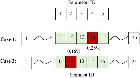
FIGURE 3. Formulated cases with damage introduced.

FIGURE 4

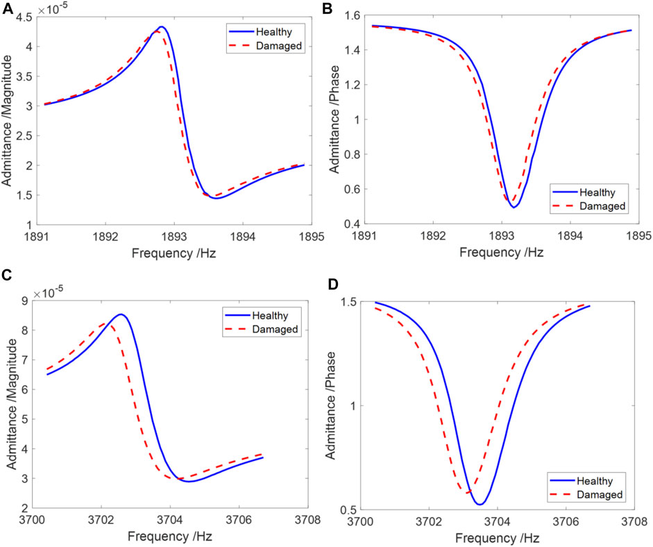
FIGURE 4. Admittance measurements over two frequency bands. (A) Magnitude (lower frequency band); (B) phase (lower frequency band); (C) magnitude (higher frequency band); and (D) phase (higher frequency band).

3.2 Damage Identification Practice on Case 1

We first examine the damage identification result of case 1 using MOMCMC. The operating parameters to execute MOMCMC are defined in Table 2. It is noted that the scaled factor is strictly calculated following the empirical formula mentioned in Section 2. The admittance measurements shown in Figure 4 are used as the evidence information to direct the inverse analysis. As can be seen clearly, the admittance indeed is sensitive to the damage, where the variations of the admittance profile and resonance are noticeable. Following the general form of the optimization problem shown in Eq. 11, we formulate the optimization problem of this inverse model updating analysis as:

$\begin{array}{l}\min \left(f_i\left(\mathbf{x}\right)\right)f_i\left(\mathbf{x}\right)={\Vert {\mathbf{Y}}_i\left(\mathbf{x}\right)-\overline{\mathbf{Y}}\Vert }^{2}i=\mathrm{1,2},\\ \text{subject}\text{to}\mathbf{x}\in \mathbf{X}\subset {\text{R}}^m,\end{array}(18)$

where ${\mathbf{Y}}_i\left(\mathbf{x}\right)$ and $\overline{\mathbf{Y}}$ are the admittance responses over ith resonant frequency from FE simulation and the respective admittance measurement under damaged structure, respectively. ${\mathbf{Y}}_i\left(\mathbf{x}\right)$ and $\overline{\mathbf{Y}}$ essentially are the vectors of complex numbers including amplitude and phase values, respectively. $\mathbf{x}$ is the m-dimensional damage vector. $\Vert .\Vert$ is the $l_2$ norm operator. Since in this research two resonant frequencies are involved for admittance evaluation, a bi-objective optimization problem is to be investigated. The sensitivity matrices indicated in Eq. 10 are computed via the finite difference method, which will be used for the admittance prediction to facilitate an efficient objective function evaluation. The uncertainties to be considered in this research mainly include the modeling inaccuracy due to the lack of knowledge and the admittance measurement inaccuracy that inevitably exists.

TABLE 2

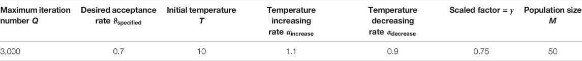
TABLE 2. Operating parameters of MOMCMC.

With the required simulation setup finalized, the inverse analysis can be implemented, and the results are obtained. Figure 5 gives the probabilistic Pareto optimal set, which essentially encompasses the deterministic optimal set. There are a total of 17 solutions identified in the deterministic Pareto optimal set, which all closely agree with the “ground truth” (i.e., 0.28% damage severity of parameter 4). The closest damage severity of parameter 4 in the optimal set is found to be nearly identical to the ground truth, only with $3.62\times {10}^{-4}\%$ difference. The result indeed illustrates the validity of the probabilistic Pareto optimal set identified. Ideally, both the numerical models and measurements are error-free, and the deterministic Pareto optimal set thus can be deemed as the final solution. In this context, the results from the probabilistic multi-objective inverse analysis are more generic. As the interested parameters are high-dimensional, the probabilistic Pareto optimal set essentially is represented by a multivariate distribution. For the sake of illustration, we project such multivariate distribution into different two-dimensional planes. To capture the main features and keep the results concise, only the two-dimensional distribution associated with parameter 4 is presented as shown in Figure 6. Obviously, due to uncertainties, many near-optimal solutions are scattered in the vicinity of the deterministic Pareto optimal set to construct the probabilistic Pareto optimal set. It is interestingly observed that the actual damage (parameter 4) in the presence of uncertainties may be identified as less severe than the one without uncertainties. Parameter 1, which is in fact damage-free, is identified as being subjected to severer damage under uncertainties than that without uncertainties. This observation indicates the high sensitivity of the identification of parameter 1 with respect to uncertainties. There may exist a boundary/envelope to truly encompass the probabilistic Pareto optimal set. Usually, the larger the population size involved, the clearer and more accurate the boundary will be captured. However, increasing the population size will increase the computational cost of MOMCMC analysis. The population size thus needs to be carefully chosen. Here, for illustration purposes, we arbitrarily generate the boundaries for all projected two-dimensional distributions of the probabilistic Pareto optimal set (Figure 6). It is noted that those boundaries in the lower dimension are built without constraints. Therefore, a valid high-dimensional boundary cannot be established because of the compatibility issue.

FIGURE 5

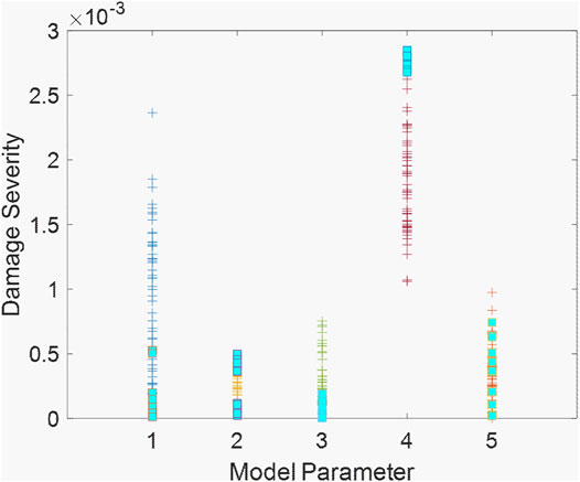
FIGURE 5. Solutions identified in the probabilistic Pareto optimal set (squared markers indicate the deterministic Pareto optimal set).

FIGURE 6

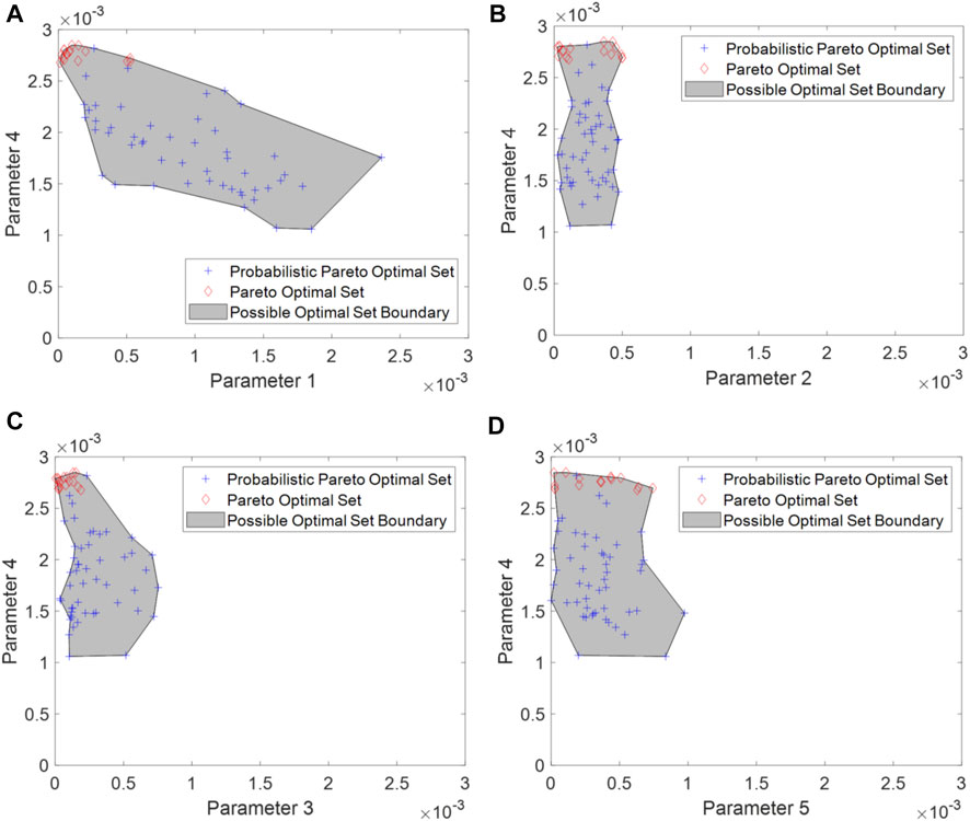
FIGURE 6. Two-dimensional illustration of the probabilistic Pareto optimal set. (A) Parameter 1 versus Parameter 4; (B) Parameter 2 versus Parameter 4; (C) Parameter 3 versus Parameter 4; and (D) Parameter 5 versus Parameter 4 (note: the Pareto optimal set boundary is roughly estimated).

Depending on the probabilistic Pareto optimal set obtained, FE simulation can be implemented accordingly to calculate the admittance response and then identify the associated probabilistic Pareto front with the estimated boundary as shown in Figure 7. Unlike the high-dimensional probabilistic Pareto optimal set, there is no compatibility issue of boundary estimation for the two-dimensional probabilistic Pareto front. The boundary of the probabilistic Pareto front is intrinsically related to the boundary of the probabilistic Pareto optimal set.

FIGURE 7

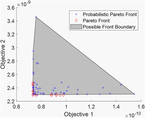
FIGURE 7. Probabilistic Pareto front (note: the Pareto front boundary is roughly estimated).

As mentioned, the convergence of MOMCMC plays an important role in ensuring a reliable optimization result. For implementation convenience, we set a relatively large maximum iteration number which is expected to lead to the MCMC convergence. There are multiple metrics that can be used to evaluate the MCMC convergence performance (Dodds and Vicini, 2004; El Adlouni et al., 2006; Roy, 2019). Among them, the autocorrelation function (ACF) is conceptually simple, which is particularly used in this research. It is mathematically formulated as (Kumar, 2019):

$r=\frac{{\displaystyle \sum _{i=1}^{M-k}\left(x_i-\overline{x}\right)\left(x_{i+k}-\overline{x}\right)}}{{\displaystyle \sum _{i=1}^M{\left(x_i-\overline{x}\right)}^2}},(19)$

where $x_i$ and $x_{i+k}$ are two samples at different time steps with k lag. $\overline{x}$ is the average of samples at all time steps in the chain. Generally, k-lag autocorrelation plots are used to diagnose and assess the MCMC convergence. The k-lag autocorrelation value decreases to zero quickly as k increases, which indicates the fast-mixing Markov chains (fast convergence). On the other hand, a large k-lag autocorrelation value for large k indicates the presence of a high degree of correlation and slow mixing of the Markov chains. In the MOMCMC, the number of Markov chains that are subjected to DE crossover is identical to the population size, that is, 50. Here, for demonstration, we only draw the autocorrelation plots of the samples in the 1st Markov chain with respect to lag as shown in Figure 8. One can notice that, in these 200-lag plots, the autocorrelation of all parameters decreases to less than 0.1, indicating that the samples generated every 200 iterations in MCMC can be deemed as independent samples. When choosing several accepted solutions in every 200 iterations as the subset of the probabilistic Pareto optimal set, the maximum number of iterations specified in the simulation (i.e., 10,000) is sufficient to cover all solutions in the probabilistic Pareto optimal set with good convergence. We further examine the convergence performance in a succinct manner, in which we only retrieve the autocorrelation value of the last lag (i.e., 200th lag) for each Markov chain, and combine the information of all chains altogether as shown in Figure 9. As can be observed, the convergence performance of Markov chains of parameter 5 is slightly inferior to that of the remaining parameters, which is consistent with the result in Figure 8. However, the overall autocorrelation degree of all Markov chains for all parameters is quite low, that is, under 0.1. This set of results illustrates that the good convergence of MCMCs can be ensured using the maximum iteration number specified in the simulation. It is therefore confirmed that the identified probabilistic Pareto optimal set and respective probabilistic Pareto front (Figures 5–7) are reliable. Putting all the aforementioned procedures together establishes the overall implementation flowchart as shown in Figure 10, which is intended for the interested readers to repurpose their own tasks using our proposed methodology.

FIGURE 8

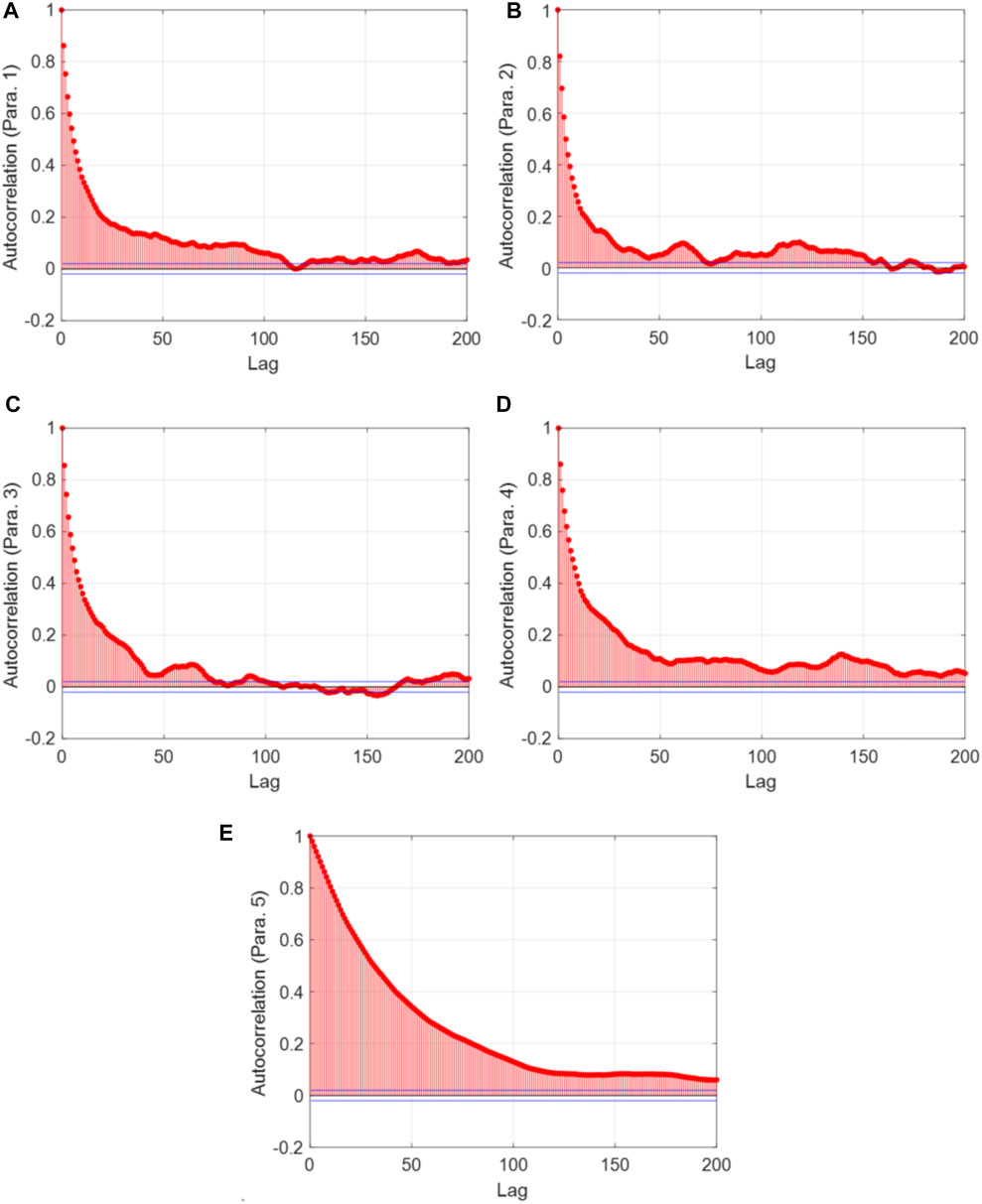
FIGURE 8. Autocorrelation of the 1st Markov chain with respect to lag. (A) Parameter 1; (B) Parameter 2; (C) Parameter 3; (D) Parameter 4; and (E) Parameter 5.

FIGURE 9

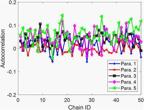
FIGURE 9. Last-lag autocorrelation values of all Markov chains.

FIGURE 10

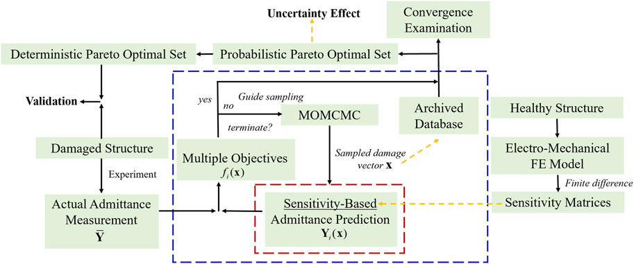
FIGURE 10. Overall implementation flow.

3.3 Additional Case (Case 2) Investigation–Identification of a Smaller Damage

In case 2, the location of damage (i.e., segment ID) changes, and the actual damage severity becomes smaller than that in case 1. Intuitively, the reduced damage severity in this case will pose the difficulty in pursuing the high accuracy of damage identification, since the identification result may be easily interfered with by uncertainties. We follow the same operating parameters tabulated in Table 2 and use the admittance measurement of the structure with the new damage introduction to execute the inverse model updating analysis. Following similar procedures, we first identify the probabilistic Pareto optimal set with many solutions as shown in Figure 11. The deterministic Pareto optimal set encompassed by the probabilistic Pareto optimal set includes 17 solutions, all of which well approach the actual damage scenario (i.e., 0.16% damage in parameter 2). The closest damage severity of parameter 2 in the optimal set is 0.0145%. While the discrepancy, that is, 0.015% between the best severity value and ground truth increases as compared to that of case 1, it is still very minor. The near-optimal solutions essentially are yielded as the consequence of uncertainties. The two-dimensional projections of the probabilistic Pareto optimal set are then given in Figure 12, where a similar observation is obtained. Parameter 2 is identified to be less severe when uncertainties are considered. In comparison, parameter 5 has the severer damage identified under uncertainties even though it is damage-free. The boundaries of scattered solutions are also estimated to reflect the uncertainty effect. Overall, the variation of solutions in this case appears to be smaller than that in case 1 (Figure 6), which may be because of the smaller true damage considered in this case. Based on the probabilistic Pareto optimal set, we can obtain the associated probabilistic Pareto front and estimate its boundary as given in Figure 13.

FIGURE 11

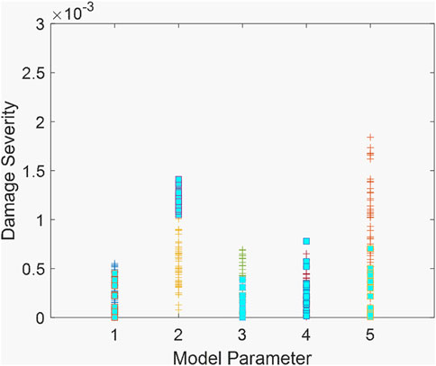
FIGURE 11. Solutions identified in the probabilistic Pareto optimal set (squared markers indicate the deterministic Pareto optimal set).

FIGURE 12

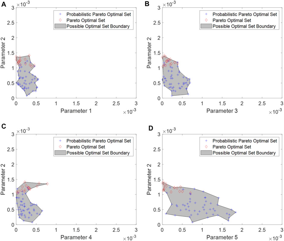
FIGURE 12. Two-dimensional illustration of the probabilistic Pareto optimal set. (A) Parameter 1 versus Parameter 4; (B) Parameter 2 versus Parameter 4; (C) Parameter 3 versus Parameter 4; and (D) Parameter 5 versus Parameter 4 (case 2).

FIGURE 13

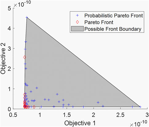
FIGURE 13. Probabilistic Pareto front (case 2).

Similarly, we then implement the MCMC convergence analysis using the autocorrelation plots. The autocorrelation plots of the 1st Markov chain are shown in Figure 14. The autocorrelation of parameter 5 is higher than those of the other parameters. Specifically, the last-lag autocorrelation value of parameter 5 is around 0.1, whereas the last-lag autocorrelation values of other parameters are all close to 0. However, a quite uniform autocorrelation decreasing trend of parameter 5 implies that further increasing lags will likely continue to de-correlate two observations. Therefore, the maximum iteration number chosen in this case should also be reasonable. The last-lag autocorrelation values of all Markov chains are given in Figure 15, consistently showing a satisfactory convergence performance.

FIGURE 14

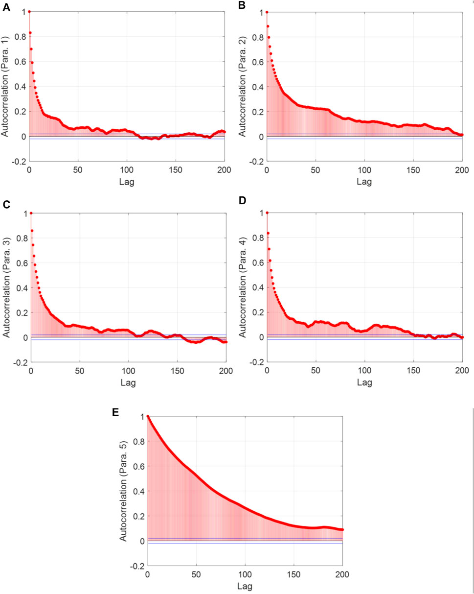
FIGURE 14. Autocorrelation of MCMC with respect to lag. (A) Parameter 1; (B) Parameter 2; (C) Parameter 3; (D) Parameter 4; and (E) Parameter 5 (case 2).

FIGURE 15

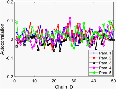
FIGURE 15. Last-lag autocorrelation values of all Markov chains (case 2).

In an ideal case without the measurement uncertainties and modeling errors, the admittance response prediction of the actual damage becomes identical to the experimental admittance measurement. The deterministic Pareto optimal set, hence, is expected to embrace the “ground truth” solution, which is already captured in the results obtained through carrying out the proposed methodology. This finding indicates the effectiveness of the proposed methodology. More importantly, the unique advantage of this methodology can be fully exploited, that is, its capability in producing the solutions which can elucidate their intrinsic correlations with respect to uncertainties. This will provide in-depth insights to guide practical damage identification that is inevitably subjected to various uncertainties.

4 Conclusion

In this research, we develop a probabilistic multi-objective finite element (FE) model updating framework built on the differential evolution Markov chain Monte Carlo (DEMC) to conduct damage identification in the presence of uncertainties. Taking advantage of the high sensitivity with respect to the damage, the piezoelectric admittance measurements are particularly used to facilitate the inverse model updating analysis. This new methodology is generic since it can yield the probabilistic Pareto optimal set that already encompasses the deterministic Pareto optimal set provided through the conventional multi-objective inverse analysis. More importantly, such a probabilistic feature also is capable of accounting for the effect of uncertainties that inevitably exist either in FE modeling or measurement when performing the multi-objective inverse analysis. Systematic case studies on a cantilever plate with experimental validation clearly illustrate the effectiveness and robustness of this proposed methodology. In addition to elucidating the uncertainty effect, the proposed methodology yields the damage severity degrees which closely match the ground truth values, only with $3.62\times {10}^{-4}\%$ and 0.015% stiffness loss discrepancies for cases 1 and 2, respectively.

Data Availability Statement

The raw data supporting the conclusion of this article will be made available by the authors, without undue reservation.

Author Contributions

KZ: conceptualization, methodology, numerical analysis and validation, and manuscript drafting and revision. YZ: numerical analysis and validation and manuscript revision. QS: experimental testing and data acquisition and manuscript revision. JT: conceptualization, methodology, manuscript revision, and supervision.

Funding

This research is supported in part by the National Science Foundation under grant CMMI—2138522 and in part by the National Science Foundation under grant CMMI—1825324.

Conflict of Interest

The authors declare that the research was conducted in the absence of any commercial or financial relationships that could be construed as a potential conflict of interest.

Publisher’s Note

All claims expressed in this article are solely those of the authors and do not necessarily represent those of their affiliated organizations, or those of the publisher, the editors and the reviewers. Any product that may be evaluated in this article, or claim that may be made by its manufacturer, is not guaranteed or endorsed by the publisher.

References

Alexandrino, P. D. S. L., Gomes, G.F., and Cunha, S. S. (2020). A Robust Optimization for Damage Detection Using Multiobjective Genetic Algorithm, Neural Network and Fuzzy Decision Making. Inverse Probl. Sci. Eng. 28 (1), 21–46. doi:10.1080/17415977.2019.1583225

CrossRef Full Text | Google Scholar

Bartle, R. G. (1995). “The Elements of Integration and Lebesgue Measure,” in The Elements of Integration and Lebesgue Measure (Hoboken, NJ, USA: John Wiley & Sons). doi:10.1002/9781118164471

CrossRef Full Text | Google Scholar

Braak, C. J. F. T. (2006). A Markov Chain Monte Carlo Version of the Genetic Algorithm Differential Evolution: Easy Bayesian Computing for Real Parameter Spaces. Stat. Comput. 16 (3), 239–249. doi:10.1007/s11222-006-8769-1

CrossRef Full Text | Google Scholar

Brooks, S., Gelman, A., and Jones, G (2011). Handbook of Markov Chain Monte Carlo. (New York: CRC Press). Chapman \& Hall/CRC Handbooks of Modern Statistical Methods

Google Scholar

Cao, M., Radzieński, M., Xu, W., and Ostachowicz, W. (2014). Identification of Multiple Damage in Beams Based on Robust Curvature Mode Shapes. Mech. Syst. Signal Process. 46 (2), 468–480. doi:10.1016/j.ymssp.2014.01.004

CrossRef Full Text | Google Scholar

Cao, P., Qi, S., and Tang, J. (2018). Structural Damage Identification Using Piezoelectric Impedance Measurement with Sparse Inverse Analysis. Smart Mat. Struct. 27 (3), 035020. IOP Publishing. doi:10.1088/1361-665X/aaacba

CrossRef Full Text | Google Scholar

Capecchi, D., Ciambella, J., Pau, A., and Vestroni, F. (2016). Damage Identification in a Parabolic Arch by Means of Natural Frequencies, Modal Shapes and Curvatures. Meccanica 51 (11), 2847–2859. doi:10.1007/s11012-016-0510-3

CrossRef Full Text | Google Scholar

Chen, Z., Zhang, R., Zheng, J., and Sun, H. (2020). Sparse Bayesian Learning for Structural Damage Identification. Mech. Syst. Signal Process. 140, 106689. doi:10.1016/j.ymssp.2020.106689

CrossRef Full Text | Google Scholar

Dodds, M. G., and Vicini, P. (2004). Assessing Convergence of Markov Chain Monte Carlo Simulations in Hierarchical Bayesian Models for Population Pharmacokinetics. Ann. Biomed. Eng. 32 (9), 1300–1313. doi:10.1114/B:ABME.0000039363.94089.08

PubMed Abstract | CrossRef Full Text | Google Scholar

El Adlouni, S., Favre, A.-C., and Bobée, B. (2006). Comparison of Methodologies to Assess the Convergence of Markov Chain Monte Carlo Methods. Comput. Statistics Data Analysis 50 (10), 2685–2701. doi:10.1016/j.csda.2005.04.018

CrossRef Full Text | Google Scholar

Khodaparast, H. H., Mottershead, J. E., and Badcock, K. J. (2011). Interval Model Updating with Irreducible Uncertainty Using the Kriging Predictor. Mech. Syst. Signal Process. 25 (4), 1204–1226. doi:10.1016/j.ymssp.2010.10.009

CrossRef Full Text | Google Scholar

Kim, J., Harne, R. L., and Wang, K. W. (2015). Enhancing Structural Damage Identification Robustness to Noise and Damping with Integrated Bistable and Adaptive Piezoelectric Circuitry. J. Vib. Acoust. 137 (1). 011003. doi:10.1115/1.4028308

CrossRef Full Text | Google Scholar

Kim, J., and Wang, K.-W. (2019). Electromechanical Impedance-Based Damage Identification Enhancement Using Bistable and Adaptive Piezoelectric Circuitry. Struct. Health Monit. 18 (4), 1268–1281. doi:10.1177/1475921718794202

CrossRef Full Text | Google Scholar

Kirkpatrick, S., Gelatt, C. D., and Vecchi, M. P. (1983). Optimization by Simulated Annealing. Science 220 (4598), 671–680. doi:10.1126/science.220.4598.671

PubMed Abstract | CrossRef Full Text | Google Scholar

Kumar, R. (2019). Machine Learning Quick Reference. Birmingham: Packt Publishing.

Google Scholar

Li, Y. (2012). MOMCMC: An Efficient Monte Carlo Method for Multi-Objective Sampling over Real Parameter Space. Comput. Math. Appl. 64 (11), 3542–3556. Elsevier Ltd. doi:10.1016/j.camwa.2012.09.003

CrossRef Full Text | Google Scholar

Magacho, E. G., Jorge, A. B., and Gomes, G. F. (2021). Inverse Problem Based Multiobjective Sunflower Optimization for Structural Health Monitoring of Three-Dimensional Trusses. Evol. Intel., 1–21. doi:10.1007/s12065-021-00652-4

CrossRef Full Text | Google Scholar

Mottershead, J. E., Link, M., and Friswell, M. I. (2011). The Sensitivity Method in Finite Element Model Updating: A Tutorial. Mech. Syst. Signal Process. 25 (7), 2275–2296. doi:10.1016/j.ymssp.2010.10.012

CrossRef Full Text | Google Scholar

Qingfu Zhang, Q., Aimin Zhou, A., and Yaochu Jin, Y. (2008). RM-MEDA: A Regularity Model-Based Multiobjective Estimation of Distribution Algorithm. IEEE Trans. Evol. Comput. 12 (1), 41–63. doi:10.1109/TEVC.2007.894202

CrossRef Full Text | Google Scholar

Roy, V. (2019). Convergence Diagnostics for Markov Chain Monte Carlo. Annu. Rev. Statistics Its Appl. 7, 387–412. doi:10.1146/annurev-statistics-031219-041300

CrossRef Full Text | Google Scholar

Shuai, Q., Zhou, K., Zhou, S., and Tang, J. (2017). Fault Identification Using Piezoelectric Impedance Measurement and Model-Based Intelligent Inference with Pre-screening. Smart Mat. Struct. 26 (4), 045007. doi:10.1088/1361-665X/aa5d41

CrossRef Full Text | Google Scholar

Storn, R., and Price, K. (1997). Differential Evolution - A Simple and Efficient Heuristic for Global Optimization over Continuous Spaces. J. Glob. Optim. 11 (4), 341–359. doi:10.1023/A:1008202821328

CrossRef Full Text | Google Scholar

Sun, H., Mordret, A., Prieto, G. A., Toksöz, M. N., and Büyüköztürk, O. (2017). Bayesian Characterization of Buildings Using Seismic Interferometry on Ambient Vibrations. Mech. Syst. Signal Process. 85, 468–486. doi:10.1016/j.ymssp.2016.08.038

CrossRef Full Text | Google Scholar

Wan, H.-P., and Ren, W.-X. (2015). Parameter Selection in Finite-Element-Model Updating by Global Sensitivity Analysis Using Gaussian Process Metamodel. J. Struct. Eng. 141 (6), 04014164. doi:10.1061/(asce)st.1943-541x.0001108

CrossRef Full Text | Google Scholar

Wang, X., and Tang, J. (2009). Damage Identification Using Piezoelectric Impedance Approach and Spectral Element Method. J. Intelligent Material Syst. Struct. 20 (8), 907–921. doi:10.1177/1045389X08099659

CrossRef Full Text | Google Scholar

Xia, Y., and Hao, H. (2003). Statistical Damage Identification of Structures with Frequency Changes. J. Sound Vib. 263 (4), 853–870. doi:10.1016/S0022-460X(02)01077-5

CrossRef Full Text | Google Scholar

Zhou, K., Shuai, Q., and Tang, J. (2014). “Adaptive Damage Detection Using Tunable Piezoelectric Admittance Sensor and Intelligent Inference,” in Volume 1: Development and Characterization of Multifunctional Materials; Modeling, Simulation and Control of Adaptive Systems; Structural Health Monitoring; Keynote Presentation. Newport, Rhode Island, USA, 8 September 2014, (New York, NY: American Society of Mechanical Engineers), doi:10.1115/SMASIS2014-7624

CrossRef Full Text | Google Scholar

Zhou, K., and Tang, J. (2021a). Structural Model Updating Using Adaptive Multi-Response Gaussian Process Meta-Modeling. Mech. Syst. Signal Process. 147, 107121. Elsevier Ltd. doi:10.1016/j.ymssp.2020.107121

CrossRef Full Text | Google Scholar

Zhou, K., and Tang, J. (2021b). Computational Inference of Vibratory System with Incomplete Modal Information Using Parallel, Interactive and Adaptive Markov Chains. J. Sound Vib. 511, 116331. doi:10.1016/j.jsv.2021.116331

CrossRef Full Text | Google Scholar

Zhou, K., and Tang, J. (2016). Highly Efficient Probabilistic Finite Element Model Updating Using Intelligent Inference with Incomplete Modal Information. J. Vib. Acoust. Trans. ASME 138 (5), 1–14. doi:10.1115/1.4033965

CrossRef Full Text | Google Scholar

Zhou, K., and Tang, J. (2015). Reducing Dynamic Response Variation Using Nurbs Finite Element-Based Geometry Perturbation. J. Vib. Acoust. Trans. ASME 137 (6), 1–11. doi:10.1115/1.4030902

CrossRef Full Text | Google Scholar

Zhu, H., Li, J., Tian, W., Weng, S., Peng, Y., Zhang, Z., et al. (2021). An Enhanced Substructure-Based Response Sensitivity Method for Finite Element Model Updating of Large-Scale Structures. Mech. Syst. Signal Process. 154, 107359. doi:10.1016/j.ymssp.2020.107359

CrossRef Full Text | Google Scholar

Zitzler, E., and Thiele, L. (1999). Multiobjective Evolutionary Algorithms: a Comparative Case Study and the Strength Pareto Approach. IEEE Trans. Evol. Comput. 3 (4), 257–271. doi:10.1109/4235.797969

CrossRef Full Text | Google Scholar