On the use of climate models for estimating the non-stationary characteristic values of climatic actions in civil engineering practice

1 Introduction

Climate change refers to the substantial variability of long-term atmospheric climate. Global warming induced by human activity has raised the global average temperature by 1°C above pre-industrial levels in 2017, likely to reach to 1.5°C around 2040 (Allen et al., 2018). The change in climate system is consequently causing variation in the frequency, intensity and, duration of climate extremes (Field and Christopher, 2012; Hao et al., 2013; Mika, 2013; van der Wiel and Bintanja, 2021). The anticipated occurrence of more climate extremes will consequently lead to a greater exposure of the structural reliability, usability, and load carrying capacity (Seneviratne et al., 2012).

Within the paper “action” refers to “loads” according to European Structural Design codes. Temporal variability describes the climate variability independently of the duration of the variation.

The climate change induced variability in climatic actions can potentially affect the design of new structures, as well as the assessment of existing structures designed in accordance with the past or current codes. Structural design codes guarantee that a structure will endure environmental loads to an acceptable risk during the design working life (Deodatis et al., 2014). It is important to note that the notional design working life serves only as a reference time period during which the structure is expected to meet its intended time-dependent performance objectives (Yu and Bull, 2006). However, it is evident from common experience that structures typically exhibit a real life well beyond the notional design working life, resulting in a greater exposure towards the climate change implications.

The structural design process is generally governed by climatic actions such as temperature, snow, and wind etc. The characteristic values of climatic actions in design codes are estimated from the extreme value analysis of past observation data (typically 40–50 years of measurements) under a stationary climate assumption i.e., no temporal variability in the statistics of extremes. Since, the estimation is based on limited meteorological observations, the possible existence of long-term trends is typically not considered. Recent studies show that climate extremes usually exhibit non-stationarity in the form of trend, shifts or a combination of both. Changes in the climate system are usually associated with the temporal variation of the statistical properties of climatic variables. While a well-established theory about the non-stationary extreme value analysis doesn’t exist to date, a general technique is the definition of non-stationary extreme value models, where the temporal dependency is expressed as a trend in the underlying extreme value distribution parameters (Coles, 2011). Although, many models exist in the literature, simple linear models are the most popular ones, where the non-stationarity is only considered in the mean while keeping the variability constant (Parey et al., 2010; Cooley et al., 2013; Katz, 2013; Renard et al., 2013; Sura, 2013; Salas and Obeysekera, 2014; Ragno et al., 2019; de Leo et al., 2021). However, a major drawback of these approaches is the lack of a physical basis and the difficulty of formulating a representative trend function (Mentaschi et al., 2016). Also, the temporal dependency of climate extremes is equally sensitive to the changes in variability than to the changes in the mean value (Katz and Brown, 1992).

To eliminate the uncertainty arising from non-stationary trend models and, to form a sound physical basis for further calculations, the use of appropriate climate models become inevitable (Croce et al., 2019). Climate models serves as a major source of information about the future climate evolution, simulating the physics of atmosphere and oceans to develop projections of climate variables (Wang et al., 2004; Rummukainen, 2010). One key aspect of the climate models is the resolution of a single cell of the geographical grid used for the simulation. As of today, the regional climate models produces output at a resolution of 10–12 km, approaching to true local scales with a promising representation of the spatial detail and extremes (Christensen and Christensen, 2007; Suklitsch et al., 2008).

The study of climate change impacts on climatic actions is a key aspect in the future evolution of structural design codes (CEN/TC 250, 2013). In this paper a general methodology to calculate the non-stationary characteristic values of climatic actions is presented. The observation data and regional climate models are analyzed to determine the climate change influence on climatic actions, providing a basis for potential amendments in the current definition of characteristic values in structural design codes. The influence of non-stationarity is explicitly discussed with respect to the design working life, quantifying the effects of climate change, and ensuring the sustainability of civil engineering infrastructure against potentially variable climatic loads.

2 Methodology

The methodology proposed for the calculation of non-stationary characteristic values of climatic actions can be summarized in the following steps (shown in Figure 1):

(1) Collection of high-resolution climate model data and extracting the time series of climate variables for the coordinates corresponding to the meteorological station.

(2) Bias-correction of the climate model data and aggregation of the climate extremes by considering seasonal variability of the climate variables.

(3) Performing non-stationary extreme value analysis and the calculation of characteristic values of climatic actions.

FIGURE 1

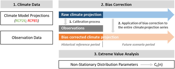
FIGURE 1. Overview of the proposed methodology for the calculation of non-stationary characteristic values of climatic actions.

2.1 Climate data

The characteristic values of climatic actions are traditionally determined from the extreme value analysis of past observation data at a point scale spatial resolution. However, the projected long-term influence of climate change can only be realistically assessed using the regional climate models. In this study, daily climate projections of the maximum temperature (T_max) in the calibration period (1951–2005) and the future scenario period (2006–2100) are extracted from the ReKliEs-De project for two representative concentration pathway scenarios i.e., RCP26 and RCP85 as shown in Table 1. The ReKliEs-DE ensemble of regional climate projections provides evaluations for Germany and the river catchment areas draining into Germany (Hübener et al., 2017). The rationale for using multi-model ensemble is that each climate model can be considered as an independent realization of the future climate evolution. The consideration of minimum and maximum multi-model ensemble improves the reliability of results by covering a bandwidth of the possible range of realizations (Tebaldi and Knutti, 2007). Since, the climate model output is typically available in the form of grids, the data is remapped to extract the time-series relative to the coordinates of a meteorological station using climate data operators (CDO) (Schulzweida et al., 2019).

TABLE 1

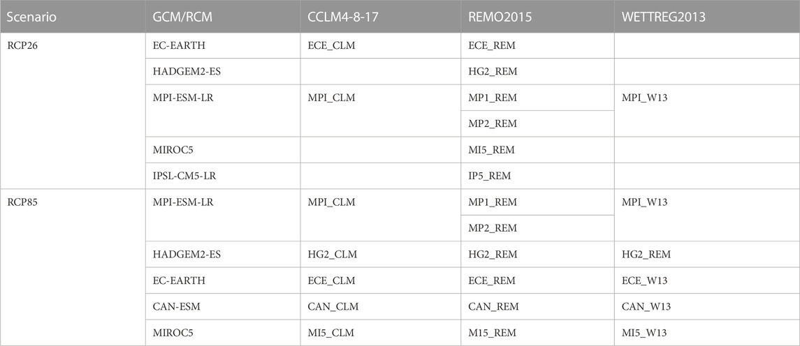
TABLE 1. List of climate models considered for analysis (Hübener et al., 2017).

2.2 Bias-correction

The use of climate model data for the calculation of characteristic values of climatic actions has two major short comings: 1) the output produced by climate models (grid) usually do not fit exactly to the underlying distribution of the relevant observation data (point scale), and 2) climate models usually produce output at large averaging duration (e.g., daily mean), while the characteristic values of climatic actions are computed using climate data at a relatively fine averaging duration (e.g., 10-min or hourly mean values).

Bias-correction is the process of scaling climate model output to account for the systematic model errors, improve fitting to the observation data, and downscaling of the climate variables to an averaging duration of interest. The correction is usually applied to the modelled mean, variance, and also to the higher moments of a distribution, with many methods now applying bias-correction to all quantiles (Hagemann et al., 2011; Hopkinson et al., 2011; Gudmundsson et al., 2012; Hempel et al., 2013; Gutmann et al., 2014; Li et al., 2014). In this study, the raw climate model data is corrected using Quantile Delta Mapping (QDM) (Cannon et al., 2015), utilizing the overlapping time-period between the climate model and observation data from the German Meteorological Service (DWD).

However, the concept of bias-correction is not undisputed. Although, these procedures can produce realistic results in certain situations, bias-correction cannot be expected to produce the baseline climate perfectly (Ehret et al., 2012). Moreover, the accuracy of bias-correction procedures relies on the length and quality of the observation data. Too few data-points and unrealistic magnitudes in the observation data can lead to the incorrect representation of the future projected output. Although, bias-correction is not a substitute of the observation data, it can still be used in the absence of reliable and long duration meteorological records. It is important to note that, even though this study uses a certain set of climate model (ReKliEs-De) and observation data (DWD) for elaboration, the methodology is independent of the data source and can be reapplied to any set of data with varying accuracy.

2.3 Aggregation of climate extremes

The annual extremes of climate variables are aggregated from the bias-corrected envelopes of climate models considering their seasonal variability. The aggregation period is different for each climate variable under consideration. For example, the annual extreme values of snow should be aggregated within a period spanning from summer to summer in two consecutive years. On the other hand, annual extreme values of maximum temperature are aggregated between winter to summer of the same year. This ensures that the resampled extreme values are mutually exclusive i.e., no two annual extremes are resampled from the same climate event.

2.4 Non-stationary characteristic values

In general, the characteristic values of climatic actions are defined for a given probability of exceedance in a certain reference period. To consider non-stationarity, the time series of annual extremes is divided into multi-year-quasi-stationary windows (n) of equal length (L-year) and applying the stationary theory to each window as shown in Figure 2A. The choice of window length depends on the severity of trend within a particular time series. The windows are shifted by 1 year from each other and fitted to a probability distribution function, leading to the computation of a series of characteristic values (c_k(n)) corresponding to the n^th quasi-stationary window.

${\mathit{c}}_{\mathit{k}}\left(\mathit{n}\right)={\mathit{F}}_{\mathit{n}}^{-\mathbf{1}}\left(\mathbf{1}-\mathit{p}\right)(1)$

where, c_k(n) is the characteristic value for p% probability of exceedance corresponding to the n^th quasi-stationary window. F⁻¹ is the inverse cumulative distribution function of user choice.

FIGURE 2

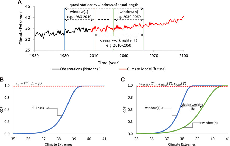
FIGURE 2. Concept of the stationary and non-stationary characteristic values: (A) definition of quasi-stationary windows for extreme value analysis; (B) stationary assumption, one distribution function; (C) non-stationary assumption, “n” distribution functions.

The exceedance probability associated with c_k(n) is expected to change due to non-stationarity during the design working life (T_L) of a structure as shown in Figures 2B, C. This transient nature makes the application and interpretation of c_k(n) in the design process rather difficult. Therefore, three possible solutions as a function of T_L are compared: a) mean characteristic value (c_k,mean), b) maximum characteristic value (c_k,max), and c) equivalent characteristic value (c_k,eq).

${\mathit{c}}_{\mathit{k},\mathit{m}\mathit{e}\mathit{a}\mathit{n}}\left(\mathit{T}\right)=\frac{\mathbf{1}}{\mathit{T}}{\displaystyle \sum }_{\mathit{n}=\mathbf{1}}^{\mathit{T}}\left[{\mathit{F}}_{\mathit{n}}^{-\mathbf{1}}\left(\mathbf{1}-\mathit{p}\right)\right](2)$

${\mathit{c}}_{\mathit{k},\mathit{max}}\left(\mathit{T}\right)=\underset{\mathit{n}=\mathbf{1},\mathit{T}}{\mathit{max}}\left[{\mathit{F}}_{\mathit{n}}^{-\mathbf{1}}\left(\mathbf{1}-\mathit{p}\right)\right](3)$

${\mathit{c}}_{\mathit{k},\mathit{e}\mathit{q}}\left(\mathit{T}\right)={\displaystyle \prod }_{\mathit{n}=\mathbf{1}}^{\mathit{T}}\left[{\mathit{F}}_{\mathit{n}}\left(\mathit{X}\le {\mathit{c}}_{\mathit{k},\mathit{e}\mathit{q}}\right)\right]={\left(\mathbf{1}-\mathit{p}\right)}^{\mathit{T}}(4)$

where, n = 1 is the reference construction year of the structure.

3 Results and discussion

The following section demonstrates the application of the proposed methodology for climate change assessment on the characteristic values of maximum temperature (T_max) in Plauen, Germany. Starting with the climate models summarized in Table 1, the raw climate model output is remapped to extract the time series corresponding to the coordinates of the local meteorological station. Each time series is then bias-corrected with respect to the hourly maximum of observation data using the quantile delta mapping while preserving relative change between quantiles (Cannon et al., 2015). Full observation data is used in order to reduce the uncertainties arising from bias-correction. The bias-corrected data is then aggregated into annual extremes considering the seasonal variability in the period spanning from January to December in accordance with section 2.3. Figure 3 shows the minimum and maximum multi-model ensemble of the annual extremes, covering the full bandwidth of all considered climate model realizations. The time series of annual extremes is subdivided into 30-year long quasi-stationary windows, shifted by 1-year from each other. In climate science, 30-years is frequently considered as a stationary period with long enough sample size to avoid uncertainty in further statistical calculations (Hennemuth et al., 2013). Each quasi-stationary window is fitted by assuming the generalized extreme value distribution (GEV) to determine the non-stationary location (µ), scale (σ) and shape (ζ) parameters.

FIGURE 3

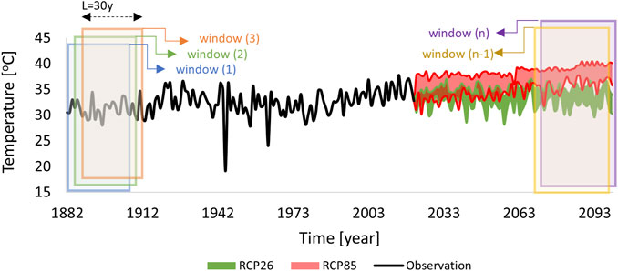
FIGURE 3. Multi-model envelope of the bias-corrected climate model projections for the maximum temperature (T_max). The quasi-stationary windows, each 30 years long are shown by bounding boxes.

The non-stationary characteristic values are calculated in accordance with Eurocode EN1990, where the characteristic values are associated with a 2% probability of exceedance (p) of the time varying part in 1-year, leading to a return period of 50-years (EN 1990/NA, 2010). Figure 4 shows the characteristic values c_k(n) of the maximum temperature calculated using Equation 1 and the distribution parameters corresponding to each quasi-stationary window respectively. The projected temperature is followed by the increasing trend in c_k(n) for RCP85 scenario (shaded red area), consequently imposing higher temperature loads on structures designed in accordance with the DIN EN 1991-1-5/NA require-ment of 37°C (dashed grey line) in the near future. Additionally, in comparison to the stationary characteristic value (dotted blue line) calculated using the observation data (1882–2021), the non-stationary c_k(n) shows a large deviation reaching to approximately ±4°C approaching the year 2100. It emphasizes the need of considering non-stationarity in the calculation of design climatic loads as well as for the regularly assessment of critical infrastructures and buildings of higher importance.

FIGURE 4

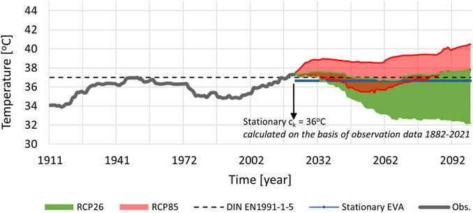
FIGURE 4. Non-stationary characteristic values c_k(n) corresponding to 2% probability of exceedance in 1-year for the maximum temperature calculated using Eq. 1.

The transient nature of c_k(n) during design working life of a structure makes it necessary to derive and adjust the values in accordance with the code defined exceedance probability of 2% in 1-year. To explain the concept, let us assume a reference construction year of 2051 for a structure with a design working life of 50-years.

Now, since, extreme events are mutually exclusive, the equivalent characteristic value c_k,eq equal to 39.9°C can be determined for an exceedance probability of 63.5% in 50-years using Equation 4 and as shown in Figure 5. It is important to note that in each quasi-stationary window the exceedance probability associated with c_k,_eq differs from 2% in 1-year because of the non-stationarity in the underlying distribution parameters. For this reason, although c_k,eq satisfies the code defined level of exceedance probability in 50-years, the corresponding 2% exceedance probability in 1-year is not necessarily satisfied in all 50-years of the design working life as shown by the red shaded area where the c_k(n) is larger than c_k,eq(50). Figures 5B, C show the range of non-exceedance probabilities, i.e., 0.84 to 1.0, computed for 39.9°C in each year of the 50-years design working life of the structure respectively. The smallest non-exceedance probability i.e., 0.84 corresponds to the last year within the design working life of the structure, implying a high chance of the occurrence of a load larger than the computed c_k(n).

FIGURE 5

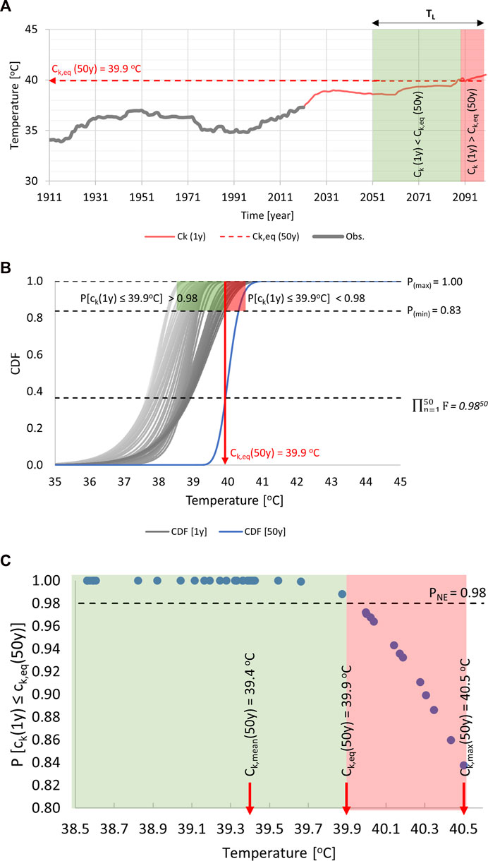
FIGURE 5. Reliability of the non-stationary characteristic values during the design working life of a structure: (A) comparison of the non-stationary characteristic values c_k(n) with the 50-year design working life characteristic values c_k,eq; (B) evaluation of 50 distribution functions over the design working life of the structure for non-stationary analysis; (C) comparison of the non-exceedance probabilities reached by c_k,eq with the target exceedance probability of 2%.

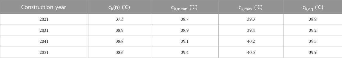
To deal with the uncertainty arising from the high exceedance probabilities associated with c_k,eq especially in the later stages of design working life, two additional methods are explored and compared. The non-conservative approach defined by Equation 2 i.e., c_k,mean derives the mean characteristic value of 39.4°C from all 50 values of c_k(n) within the design working life of the structure. On the other hand, the conservative approach defined by Equation 3 i.e., c_k,max takes the maximum of all 50 values of c_k(n) within the design working life of a structure as the governing characteristic value equal to 40.5°C.

The characteristic values derived using the three approaches for different reference construction years starting from 1911 till 2051 are compared in Figure 6; Table 2. The three approaches lead to a maximum difference of 3°C in the characteristic values for both RCP scenarios but in different years. This difference might be crucial for a temperature sensitive structure and therefore must be considered in the design process as well as regular assessment of critical infrastructures and buildings to minimize the adverse effects of increased temperature loads.

FIGURE 6

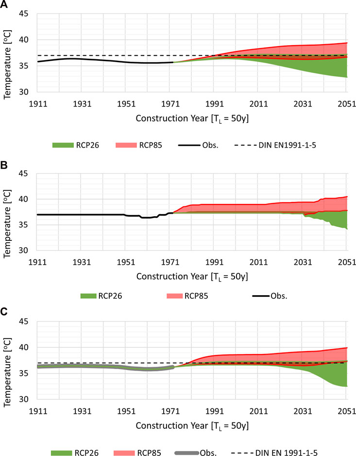
FIGURE 6. Comparison of the non-stationary characteristic values determined using different methods for a design working life of 50-years: (A) c_k,_mean with comparatively non-conservative values; (B) c_k,_max with comparatively conservative values; (C) c_k,_eq satisfying the code defined exceedance probability in 50 years i.e., 1-(1-0.02)⁵⁰.

TABLE 2

TABLE 2. Non-stationary characteristic values for the presented example using Eqs 1–4.

4 Conclusion

This paper presents a general methodology to evaluate the climate change impacts on characteristic values of climatic actions by using observations together with the climate model data. The idea is relevant since the representative values of climate actions in current structural design codes are based on the analysis of past observation data under the hypothesis of stationary climate which ultimately disregards the potential effects of climate change. The annual extremes of climate variables are extracted from a climate model ensemble and are corrected with respect to the observation data using state-of-the-art bias correction procedures. Extreme value analysis is performed using the GEV distribution and the results are presented in the form of time varying characteristic values for a design working life of 50 years. The anticipated increase of most climate extremes from climate model projections towards the end of the 21st century will ultimately result in stronger non-stationary trends especially for longer intended design working life e.g., 100-years.

Since, the global temperature is on the rise, it is expected that the characteristic values of T_max will increase in the future years. The overlapping portion of the results between RCP26 and RCP85 in Figures 4, 6 indicate the uncertainty linked to the bandwidth of output produced by an envelope of climate models. The validity of characteristic values employed in the current structural codes is discussed relative to the non-stationary characteristic values computed using the proposed methodology.

The reliability of results obtained using the presented methodology is highly influenced by the quality of observation and modelled datasets. The trend in extreme value analysis is directly introduced from the climate projections. Therefore, it is necessary to take into account the uncertainties inherent with using the output produced by climate models, where too few observation data points can result in unrealistic bias-correction of the simulated climate projections. The reliability and confidence in the bias-correction can be significantly improved by acquiring longer observation datasets.

The methodology developed provides a general guideline for the assessment of climatic actions based on climate model projections. The results indicate that the characteristic values specified in current structural design codes may not be valid under the changing climate and may ultimately reduce the intended design working life of existing and new structures. It must be mentioned that a wider field of application and improvements can be foreseen for the proposed methodology, such as: accounting for the combination factors of correlated climate variables, and implementation of updated climate projections and advanced stochastic techniques.

Data availability statement

The datasets presented in this article are not readily available because the climate data supporting this research article are from previously reported studies and datasets, which have been cited. The processed data are available from the corresponding author upon request. Requests to access the datasets should be directed to lars.abrahamczyk@uni-weimar.de.

Author contributions

LA and AU were involved in all steps of the paper preparation, from the draft, final version of the paper, revision, reading, corrections, approval, and submitted version. AU realized all necessary analysis.

Funding

This research is supported within framework of the project “Auswirkungen des Klimawandels auf Gebäude und Quartiere—Strukturelle Integrität, Raumklima und Energieeffizienz” by the Free State of Thuringia with funding from the European Social Funds (2019 FGR 0096). We acknowledge support from the German Research Foundation (DFG) and Bauhaus-Universität Weimar within the program of Open Access Publishing.

Conflict of interest

The authors declare that the research was conducted in the absence of any commercial or financial relationships that could be construed as a potential conflict of interest.

Publisher’s note

All claims expressed in this article are solely those of the authors and do not necessarily represent those of their affiliated organizations, or those of the publisher, the editors and the reviewers. Any product that may be evaluated in this article, or claim that may be made by its manufacturer, is not guaranteed or endorsed by the publisher.

References

Allen, M. R., Dube, O. P., Solecki, W., Aragón-Durand, F., Cramer, W., Humphreys, S., et al. (2018). “Framing and context,” in Global Warming of 1.5°C. An IPCC Special Report on the impacts of global warming of 1.5°C above pre-industrial levels and related global greenhouse gas emission pathways. the context of strengthening the global response to the threat of climate change, sustainable development, and efforts to eradicate poverty, Press.

Google Scholar

Cannon, A. J., Sobie, S. R., and Murdock, T. Q. (2015). Bias correction of GCM precipitation by quantile mapping: How well do methods preserve changes in quantiles and extremes? J. Clim. 28, 6938–6959. doi:10.1175/jcli-d-14-00754.1

CrossRef Full Text | Google Scholar

CEN/TC 250 (2013), Response to mandate M/515—towards a, Second-Generation of Eurocodes.

Google Scholar

Christensen, J. H., and Christensen, O. B. (2007). A summary of the PRUDENCE model projections of changes in European climate by the end of this century. Clim. Change 81, 7–30. doi:10.1007/s10584-006-9210-7

CrossRef Full Text | Google Scholar

Coles, S. (2011). An introduction to statistical modeling of extreme values. London: Springer.

Google Scholar

Cooley, D. (2013). “Extremes in a changing climate,” in Detection, analysis and uncertainty. Editors A. AghaKouchak, D. Easterling, K. Hsu, S. Schubert, and S. Sorooshian (Dordrecht: Springer Netherlands), 97–114.

CrossRef Full Text | Google Scholar

Croce, P., Formichi, P., and Landi, F. (2019). Climate change: Impacts on climatic actions and structural reliability. Appl. Sci. 9, 5416. doi:10.3390/app9245416

CrossRef Full Text | Google Scholar

de Leo, F., Besio, G., Briganti, R., and Vanem, E. (2021). Non-stationary extreme value analysis of sea states based on linear trends. Analysis of annual maxima series of significant wave height and peak period in the Mediterranean Sea. Coast. Eng. 167, 103896. doi:10.1016/j.coastaleng.2021.103896

CrossRef Full Text | Google Scholar

Deodatis, G., Ellingwood, B. R., and Frangopol, D. M. (2014). Safety, reliability, risk and life-cycle performance of structures and infrastructures. Boca Raton: CRC Press.

Google Scholar

Ehret, U., Zehe, E., Wulfmeyer, V., Warrach-Sagi, K., and Liebert, J. (2012). HESS Opinions "Should we apply bias correction to global and regional climate model data? Hydrol. Earth Syst. Sci. 16, 3391–3404. doi:10.5194/hess-16-3391-2012

CrossRef Full Text | Google Scholar

EN 1990/NA (2010), DIN EN 1990/NA:2010-12, National Annex—Nationally determined parameters—Eurocode: Basis of structural design. Berlin: Beuth Verlag GmbH.

Google Scholar

Field, C. B. (2012). “Managing the risks of extreme events and disasters to advance climate change adaptation,” in Special report of the intergovernmental panel on climate change. Editor B. Christopher (Cambridge University Press). Cambridge.

Google Scholar

Gudmundsson, L., Bremnes, J. B., Haugen, J. E., and Engen-Skaugen, T. (2012). Technical note: Downscaling RCM precipitation to the station scale using statistical transformations – A comparison of methods. Hydrol. Earth Syst. Sci. 16, 3383–3390. doi:10.5194/hess-16-3383-2012

CrossRef Full Text | Google Scholar

Gutmann, E., Pruitt, T., Clark, M. P., Brekke, L., Arnold, J. R., Raff, D. A., et al. (2014). An intercomparison of statistical downscaling methods used for water resource assessments in the United States. Water Resour. Res. 50, 7167–7186. doi:10.1002/2014wr015559

CrossRef Full Text | Google Scholar

Hagemann, S., Chen, C., Haerter, J. O., Heinke, J., Gerten, D., and Piani, C. (2011). Impact of a statistical bias correction on the projected hydrological changes obtained from three GCMs and two hydrology models. J. Hydrometeorol. 12, 556–578. doi:10.1175/2011jhm1336.1

CrossRef Full Text | Google Scholar

Hao, Z., AghaKouchak, A., and Phillips, T. J. (2013). Changes in concurrent monthly precipitation and temperature extremes. Environ. Res. Lett. 8, 034014. doi:10.1088/1748-9326/8/3/034014

CrossRef Full Text | Google Scholar

Hempel, S., Frieler, K., Warszawski, L., Schewe, J., and Piontek, F. (2013). A trend-preserving bias correction – The ISI-mip approach. Earth Syst. Dynam. 4, 219–236. doi:10.5194/esd-4-219-2013

CrossRef Full Text | Google Scholar

Hennemuth, B., Bender, S., Bülow, K., Dreier, N., and Schoetter, R. (2013). “Statistical methods for the analysis of simulated and observed climate data, applied in projects and institutions dealing with climate change impact and adaptation, 135 S,”. Technical Report.

Google Scholar

Hopkinson, R. F., McKenney, D. W., Milewska, E. J., Hutchinson, M. F., Papadopol, P., and Vincent, L. A. (2011). Impact of aligning climatological day on gridding daily maximum–minimum temperature and precipitation over Canada. J. Appl. Meteorology Climatol. 50, 1654–1665. doi:10.1175/2011jamc2684.1

CrossRef Full Text | Google Scholar

Hübener, H., Bülow, K., Fooken, C., Früh, B., Hoffmann, P., Höpp, S., et al. (2017). ReKliEs-de ergebnisbericht.

Google Scholar

Katz, R. W., and Brown, B. G. (1992). Extreme events in a changing climate: Variability is more important than averages. Clim. Change 21, 289–302. doi:10.1007/bf00139728

CrossRef Full Text | Google Scholar

Katz, R. W. (2013). Extremes in a changing climate. Dordrecht: Springer, 15–37.

CrossRef Full Text | Google Scholar

Li, C., Sinha, E., Horton, D. E., Diffenbaugh, N. S., and Michalak, A. M. (2014). Joint bias correction of temperature and precipitation in climate model simulations. J. Geophys. Res. Atmos. 119 (13), 1315–13162. doi:10.1002/2014jd022514

CrossRef Full Text | Google Scholar

Mentaschi, L., Vousdoukas, M., Voukouvalas, E., Sartini, L., Feyen, L., Besio, G., et al. (2016). Non-stationary extreme value analysis: A simplified approach for earth science applications. Hydrology Earth Syst. Sci. Discuss. doi:10.5194/hess-2016-65

CrossRef Full Text | Google Scholar

Mika, J. (2013). Changes in weather and climate extremes: Phenomenology and empirical approaches. Clim. Change 121, 15–26. doi:10.1007/s10584-013-0914-1

CrossRef Full Text | Google Scholar

Parey, S., Hoang, T. T. H., and Dacunha-Castelle, D. (2010). Different ways to compute temperature return levels in the climate change context. Environmetrics 21, 698–718. doi:10.1002/env.1060

CrossRef Full Text | Google Scholar

Ragno, E., AghaKouchak, A., Cheng, L., and Sadegh, M. (2019). A generalized framework for process-informed nonstationary extreme value analysis. Adv. Water Resour. 130, 270–282. doi:10.1016/j.advwatres.2019.06.007

CrossRef Full Text | Google Scholar

Renard, B., Sun, X., and Lang, M. (2013). in Extremes in a changing climate. Editor A. AghaKouchak (Dordrecht: Springer), 39–95.

CrossRef Full Text | Google Scholar

Rummukainen, M. (2010). State-of-the-art with regional climate models. Wiley Interdiscip. Rev. Clim. Change 1, 82–96.

CrossRef Full Text | Google Scholar

Salas, J. D., and Obeysekera, J. (2014). Revisiting the concepts of return period and risk for nonstationary hydrologic extreme events. J. Hydrol. Eng. 19, 554–568. doi:10.1061/(asce)he.1943-5584.0000820

CrossRef Full Text | Google Scholar

Schulzweida, U., Kronblueh, L., and ReinhardBudich, G. C. (2019). Climate data operators.

Google Scholar

Seneviratne, S. I., Nicholls, N., Easterling, D., Goodess, C. M., Kanae, S., Kossin, J., et al. (2012). “Changes in climate extremes and their impacts on the natural physical environment,” in Managing the risks of extreme events and disasters to advance climate change adaptation. A special report of working groups I and II of the intergovernmental panel on climate change (IPCC) (Cambridge, UK, New York, NY, USA: Cambridge University Press).

Google Scholar

Suklitsch, M., Gobiet, A., Leuprecht, A., and Frei, C. (2008). High resolution sensitivity studies with the regional climate model CCLM in the alpine region. metz 17, 467–476. doi:10.1127/0941-2948/2008/0308

CrossRef Full Text | Google Scholar

Sura, P. (2013). Extremes in a changing climate. Dordrecht: Springer, 181–222.

CrossRef Full Text | Google Scholar

Tebaldi, C., and Knutti, R. (2007). The use of the multi-model ensemble in probabilistic climate projections. Philosophical Trans. Ser. A, Math. Phys. Eng. Sci. 365, 2053–2075. doi:10.1098/rsta.2007.2076

PubMed Abstract | CrossRef Full Text | Google Scholar

van der Wiel, K., and Bintanja, R. (2021). Contribution of climatic changes in mean and variability to monthly temperature and precipitation extremes. Commun. Earth Environ. 2, 1–11. doi:10.1038/s43247-020-00077-4

CrossRef Full Text | Google Scholar

Wang, Y., Leung, L. R., McGREGOR, J. L., Lee, D.-K., Wang, W.-C., Ding, Y., et al. (2004). Regional climate modeling: Progress, challenges, and prospects. J. Meteorological Soc. Jpn. 82, 1599–1628. doi:10.2151/jmsj.82.1599

CrossRef Full Text | Google Scholar

Yu, C. W., and Bull, J. W. (2006). Durability of materials and structures in building and civil engineering.

Google Scholar