An acceleration-oriented form of simple piecewise linearisation in time series to assess seismically damaged structures

1 Introduction

Structural health monitoring is a critical subject for the maintenance of structural systems in various engineering fields (e.g., aerospace, mechanical, and civil engineering) (Farrar and Worden 2006). When an abnormality occurs within a system, the monitoring process is expected to detect its occurrence, location, and severity as promptly as possible (Brownjohn 2007). Such abnormalities occur more frequently during natural disasters than in normal times. A strong earthquake can cause significant structural damage to structures in a broad area. Thus, efficient structural monitoring techniques are required in the earthquake engineering field to quickly detect seismic structural damage (Fujino et al., 2019).

Therefore, various monitoring techniques have been developed based on the structural vibration data acquired from measurement sensors (Balsamo and Betti 2015; Nagarajaiah and Yang 2017). This vibration-based monitoring scheme can minimise human effort during emergencies caused by earthquakes and uses either a data- or model-based approach. The data-based approach finds abnormalities only from structural vibration data by utilising advanced signal processing techniques (e.g., wavelet transform (Nagarajaiah and Basu B 2009; Beskhyroun et al., 2011), machine learning [Ying et al., 2013), or pattern recognition (Sohn et al., 2001)]. Because of these features, this approach is suitable for structures that cannot be simply modelled, or for cases in which some structural responses are missing.

The model-based approach is particularly effective for structures that can be reasonably demonstrated by some models, and the models are used to find suitable parameters from structural responses, including input and output data. A frequency response function (FRF) based on modal analysis (Hearn and Testa 1991; Doebling et al., 1996; Brownjohn 2007; Ji et al., 2011), is classified as a model-based approach in the frequency domain. As FRF requires an excitation containing a wide range of frequency components (e.g., band-limited white noise), it is suitable for monitoring structures in laboratories.

A class of prediction error methods (Ljung 1998) are also classified into a model-based approach. These methods were originally established as system identification tools for the classical control theory on single-input single-output systems and have also been employed for monitoring structural buildings (Huang 2001; Neild et al., 2003; Lu and Gao 2005; Nair et al., 2006; Gul and Catbas 2011; Roy et al., 2015). These methods provide modal parameters (frequency, damping, modal shape) from the time-history data of structural responses, including its excitation, and the requirement for excitation is more relaxed than that in FRF. Similarly, subspace system identification methods (Katayama 2005), which were established for modern control theory on multi-input multi-output systems, are actively investigated for monitoring civil structures (Xiao et al., 2001; Carden and Mita 2011; Wu et al., 2016; Shokravi et al., 2020).

Monitoring techniques that provide modal parameters allow us to observe changes before and after an earthquake event, which are commonly employed as an index of seismic damage in earthquake engineering (Ntotsios et al., 2009; Vidal et al., 2014; Hwang and Lignos 2018); Sivori et al., 2022). To observe the change during seismic excitation, time-variant modal parameters have also been identified (Tobita 1996; Moaveni and Asgarieh 2012; Ikeda 2016; Astroza et al., 2018). However, in general, the modal parameters are affected by the entire condition of the structures and are insensitive to the individual conditions of the structural components (Xie et al., 2018). Thus, direct identification of physical parameters, such as the damping and stiffness coefficients in structures is required to assess the individual conditions of the structural components (Kim and Lynch 2012; Xie et al., 2018), and they are occasionally described in the time history (Kang et al., 2005; Kuleli and Nagayama 2020). Hereafter, the damping and stiffness coefficients are referred to as physical parameters to distinguish them from modal parameters.

In the field of structural health monitoring, the least-squares method is commonly employed in time-domain inversion (TDI), which estimates the unknown parameters of a structure by inverting its equation of motion together with its responses. Its effectiveness in linear structural systems has been well demonstrated (Kang et al., 2005; Shintani et al., 2017). However, for nonlinear structures, it has been mainly aimed at estimating the nonlinear hysteretic loops rather than time-varying physical parameters (Toussi and Yao 1983; Masri et al., 1987a; Masri et al., 1987b; Agbabian et al., 1991; Kitada 1998; Shintani et al., 2020).

To estimate time-varying parameters in nonlinear structures, we recently developed a simple piecewise linearisation in time series (SPLiTS) to functionalise TDI for the estimation (Enokida and Kajiwara 2020). SPLiTS, linearises a nonlinear structure piecewise based on the displacement data in which its central point shift component (e.g., residual deformation in a seismically damaged structure) is intentionally minimised. Its effectiveness was validated using experimental data of a single-storey steel frame tested for nonlinear signal-based control (Enokida et al., 2014; Enokida 2019; Enokida and Kajiwara 2019) and a full-scale three-storey steel structure (Mizushima et al., 2018) conducted at E-Defense (Nakashima et al., 2018). In the examination, SPLiTS reasonably estimated the time-varying physical parameters of the seismically damaged structures. In addition, the parameters described in the time history were effective in calculating the structural energy absorption, which is closely linked to the seismic structural damage.

The original SPLiTS requires acceleration and displacement data to be measured extensively (Enokida and Kajiwara 2020). This strict requirement is satisfied only in laboratory experiments with measurement sensors that can sufficiently cover the amplitude range of displacement and acceleration responses. However, experiments with severe excitations occasionally show unexpectedly large displacements, resulting in saturation of the measured data and the original form cannot handle these improper measurement cases. To relax the requirement and address such improper displacement measurement cases, a form independent from the displacement measurement is required. As SPLiTS is based on simple techniques (i.e., piecewise linearisation and time-domain inversion) for the estimation of time-varying physical parameters, the new form should also align with the simplicity.

To enhance the practicality of SPLiTS and maintain its simplicity, this study introduces an acceleration-oriented form based on basic signal processing techniques: integrations of acceleration and a multi-pass moving-average filtering technique. In this new form, the displacement and velocity are calculated using integrals of the measured acceleration and the unwanted distortion generated during this stage is removed by the multi-pass moving filtering technique, in which moving-average filters are applied to the data multiple times. As the new form minimises the effect of the distortion, including the information on residual deformation, it cannot accurately provide structural hysteresis, which are commonly used to observe energy absorptions in seismically damaged structures. Instead, the new form can directly calculate the structural energy absorption.

This study compares the new form of SPLiTS to the original by applying them to experimental data of a three-storey steel structure tested at E-Defense. This experimental series was selected because it has an improper displacement measurement case due to an extremely large displacement in the first storey, allowing us to examine both forms for an improper case. Hereafter, the original SPLiTS is referred to as SPLiTS4ad (acceleration and displacement) and the new form is referred to as SPLiTS4a (acceleration).

The remainder of this paper is organised as follows: Section 2 describes the new form, SPLiTS4a, along with the moving-average filtering technique and its use for structural condition assessment. Section 3 examines the effectiveness of SPLiTS4a by applying it to experimental data and discusses the structural deterioration caused by numerous seismic excitations. Finally, Section 4 presents the conclusions of the study.

2 Simple piecewise linearisation in time series

SPLiTS was developed for the TDI approach to estimate the time-varying physical parameters of a nonlinear structure by inverting its structural responses. Its original form, SPLiTS4ad, requires measured acceleration and displacement data, and its velocity is estimated using a composite filter for both (Stoten 2001). To enhance the practicality of SPLiTS, this study introduces a new form, SPLiTS4a, which relies only on the measured acceleration response data.

The principles of SPLiTS are summarised in Section 2.1, and the SPLiTS4a response estimation from acceleration data is detailed in Section 2.2. The utilisation of the estimated physical parameters for the structural condition assessment is discussed in Section 2.3.

2.1 Principles of SPLiTS to estimate time-varying physical parameters

We briefly describe the principles of SPLiTS and the procedures used to estimate the time-varying physical parameters of seismically damaged structures.

2.1.1 Principles of SPLiTS

To begin, we first describe the influence of a central-point shift component, which is an offset or residual deformation in the equation of motion of the displacement response of a structure post-earthquake. Additionally, the physical meaning of the different amplitudes and durations within a displacement response of a nonlinear structure is also discussed, as these features are closely associated with the development of SPLiTS (Enokida and Kajiwara 2020).

When a single-degree-of-freedom (SDOF) linear structure excited by an external force, its equation of motion without the central-point shift is described by:

$m\ddot{x}\left(t\right)+c\dot{x}\left(t\right)+kx\left(t\right)=f\left(t\right)(1)$

where {m, c, k} is the set of the mass, damping, and stiffness coefficients, respectively; x is the relative displacement, equal to the inter-storey drift in the case of an SDOF structure; f is the external force and t is the time variable.

An SDOF linear structure having a constant central-point shift x_c in its displacement is described by:

$m\ddot{x}\left(t\right)+c\dot{x}\left(t\right)+k\left(x\left(t\right)-x_c\right)=f\left(t\right)(2)$

By employing the coordinate of $x^{*}\left(t\right)=x\left(t\right)-x_c$, Eq. 2 can be rewritten as:

$m{\ddot{x}}^{*}\left(t\right)+c{\dot{x}}^{*}\left(t\right)+k{x}^{*}\left(t\right)=f\left(t\right)(3)$

Apart from the notation of *, Eq. 3 is identical to Eq. 1. In addition, Eq. 3 even holds for a structure having a time-varying central-point shift: ${\dot{x}}_c\left(t\right)$, particularly at ${\dot{x}}_c\left(t\right)\approx 0$, because it leads to ${\dot{x}}^{*}\left(t\right)\approx \dot{x}\left(t\right)$ and ${\ddot{x}}^{*}\left(t\right)\approx \ddot{x}\left(t\right)$. This indicates that the introduction of the coordinate $x^{*}\left(t\right)$ allows us to handle the structure having the shift component as an equivalent structure without a shift component.

When a displacement response consisting of n sets of half-cyclic waves, as shown in Figure 1, is obtained from a nonlinear structure, the amplitude and duration of each half-cyclic wave contain essential information of the structure, particularly for the case of A₁≠A₂≠···≠A_n and T₁≠T₂≠···≠T_n. Different amplitudes can indicate a structure’s non-linearity as it is closely related to the amplitude of the responses, whereas, different durations would demonstrate variations of the stiffness within the structure.

FIGURE 1

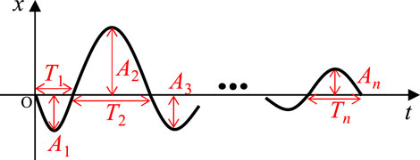
FIGURE 1. Displacement response of a structure.

These considerations motivated the development of SPLiTS, which minimises the effect of the central-point shift component in displacement responses and handles a nonlinear structure as a set of linearised structures, based on the number of half-cyclic waves in the displacement response. SPLiTS has been developed for estimating the time-varying physical parameters of nonlinear structures using TDI, based on the following four principals:

P1. SPLiTS minimises central-point shift components in the displacement response data $x\left(t\right)$, and generates new data with minimised components $x^{*}\left(t\right)$. The residual deformation observed in severely damaged structures and distortion generated by the integral of the measured acceleration data are typical examples of central-point shifts.

P2. Based on each half-cyclic wave in the new displacement data $x^{*}\left(t\right)$, SPLiTS regards a nonlinear structure as a set of linearised structures. The physical parameters of the linearised structures are estimated by TDI, and these estimates equivalently demonstrate the time-varying physical parameters of the nonlinear structure.

P3. To exclude data associated with minor structural vibrations, SPLiTS selects the effective data for TDI using the following criteria: $\left|x^{*}\left(t\right)\right|\ge {\epsilon }_d$ or $\left|{\dot{x}}^{*}\left(t\right)\right|\ge {\epsilon }_v$, where ε_d and ε_v are the thresholds for the displacement and velocity responses, respectively.

P4. To focus on half-cyclic waves with a sufficient number of steps, SPLiTS ignores half-cyclic waves lasting for less than n₀·dt s, where n₀ is the threshold for the number of steps, and dt is the sampling time interval of the measurement. This process is equivalent to ignoring the frequency components over 1/(2n₀·dt) Hz, indicating that n₀ can be roughly determined from the frequencies of interest.

P1 and P2 are fundamental for estimating the time-varying physical parameters. P3 and P4 are the criteria for extracting major structural response data and minimising noise within the data for reliable estimation using TDI.

SPLiTS is based on the premise that structural responses of the displacement $x\left(t\right)$, velocity $\dot{x}\left(t\right)$ and acceleration $\ddot{x}\left(t\right)$ are given; however, in practice, the acquisition of these data is not a simple task. In this regard, SPLiTS4ad is based on the estimation of the velocity response from the measured acceleration and displacement, while SPLiTS4a is based on the estimation of the velocity and displacement from the measured acceleration. As SPLiTS4a only relies on the measured acceleration, its measurement cost is lighter than that of SPLiTS4ad. As a result, SPLiTS4a has more signal processing procedures for estimating the required responses than SPLiTS4ad. These features are summarised in Table 1.

TABLE 1

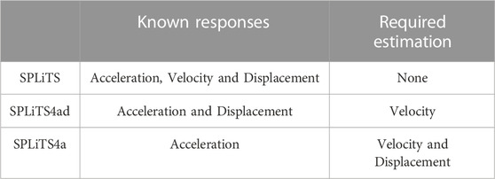
TABLE 1. Types of SPLiTS.

2.1.2 Estimation of time-varying physical parameters

The estimation of physical parameters based on SPLiTS is exemplified by an N-storey structure that can be modelled by a lumped-mass system with N masses. The equation of motion for the ith sotrey can be described by:

$m_i{\ddot{x}}_i\left(t\right)+f_{ci}\left(t\right)+f_{ki}\left(t\right)=-m_i{\ddot{x}}_g\left(t\right)+f_{i+1}\left(t\right)(4)$

where i = 1, ∙∙∙, N; x_g is the ground displacement; {m_i, x_i, f_ci, f_ki} is the set of the mass, relative displacement, damping force, and restoring force of the ith storey, respectively; and $f_i\left(t\right)=-{\displaystyle \sum }_{j=i}^N{m}_j\left({\ddot{x}}_j\left(t\right)+{\ddot{x}}_g\left(t\right)\right)$ and $f_{N+1}\left(t\right)=0$. For a linear system with constant damping and stiffness on each storey, the damping and restoring forces in Eq. 4 are described as $f_{ci}\left(t\right)=c_i\left({\dot{x}}_i\left(t\right)-{\dot{x}}_{i-1}\left(t\right)\right)$, $f_{ki}\left(t\right)=k_i\left(x_i\left(t\right)-x_{i-1}\left(t\right)\right)$, and x₀(t) = 0.

By introducing the inter-storey drift coordinate to the linear system governed by Eq. 4, the equation of motion for the ith storey becomes:

$c_i{\dot{\widehat{x}}}_i\left(t\right)+k_i{\widehat{x}}_i\left(t\right)={\widehat{f}}_i\left(t\right)(5)$

where ${\widehat{f}}_i\left(t\right)=f_i\left(t\right)$ and ${\widehat{x}}_i\left(t\right)=x_i\left(t\right)-x_{i-1}\left(t\right)$. When this system exhibits time-varying damping and stiffness on the ith storey, Eq. 5 can be rewritten as:

$c_i\left(t\right){\dot{\widehat{x}}}_i\left(t\right)+k_i\left(t\right){\widehat{x}}_i\left(t\right)={\widehat{f}}_i\left(t\right)(6)$

SPLiTS equivalently estimates the physical parameters $\left\{c_i\left(t\right),k_i\left(t\right)\right\}$ from its responses $\left\{{\dot{\widehat{x}}}_i\left(t\right),{\widehat{x}}_i\left(t\right),{\widehat{f}}_i\left(t\right)\right\}$ by piecewise linearisation of the structure governed by Eq. 6. The linearisation is performed on half-cyclic waves in the displacement data containing the minimum central-point shift components. When the response data with minimised central-point shift components $\left\{{\dot{\widehat{x}}}_i^{*}\left(t\right),{\widehat{x}}_i^{*}\left(t\right)\right\}$ are given in addition to its external force ${\widehat{f}}_i\left(t\right)$, the piecewise linearised structure for the lth half-cyclic wave consisting of n_l (>n₀) steps is described by:

${\widehat{f}}_i\left(t\right)\approx c_i^{*}{\dot{\widehat{x}}}_i^{*}\left(t\right)+k_i^{*}{\widehat{x}}_i^{*}\left(t\right)\left(t_l<t<t_l+\mathit{\Delta }{t}_l\right),(7)$

where {c_i^*, k_i^*} is the set of damping and stiffness in the linearised structure, respectively, and {t_l, Δt_l (=n_l∙dt)} is the set of the initial timestamp and duration of the lth half-cyclic wave, respectively. The physical parameters in Eq. 7 can be estimated using the following inversion:

${\mathbf{P}}_l={\left({\mathbf{Q}}_l^T{\mathbf{Q}}_l\right)}^{-1}{\mathbf{Q}}_l^T{\mathbf{F}}_l,(8)$

where ${\mathbf{P}}_l\left({\mathbb{R}}^{2\times 1}\right)=\left[\begin{array}{l}{c_i}^{*}\\ {k_i}^{*}\end{array}\right]$; ${\mathbf{Q}}_l\left(\in {\mathbb{R}}^{n_l\times 2}\right)=\left[\begin{array}{c}{\dot{\widehat{x}}}_i\left(t_l\right)\\ ⋮\\ {\dot{\widehat{x}}}_i\left(t_l+\Delta t_l\right)\end{array}\begin{array}{c}{\widehat{x}}_i\left(t_l\right)\\ ⋮\\ {\dot{\widehat{x}}}_i\left(t_l+\Delta t_l\right)\end{array}\right]$; ${\mathbf{F}}_l\left(\in {\mathbb{R}}^{n_l\times 1}\right)=\left[\begin{array}{c}{\widehat{f}}_i\left(t_l\right)\\ ⋮\\ {\widehat{f}}_i\left(t_l+\Delta t_l\right)\end{array}\right]$; $\mathbb{R}$ is the set of real numbers, and its superscript is the dimension of the matrix. The estimated parameters are stored in $\left\{{c_i}^{*}\left(t\right),{k_i}^{*}\left(t\right)\right\}$ as the representation of its entire duration, $\mathit{\Delta }{t}_l$. In computations, Eq. 8 should be solved by using a pseudo inversion method to enhance its accuracy.

By repeating the procedure in Eq. 8 to the other half-cyclic waves, the time-varying physical parameters in Eq. 6 can be equivalently obtained as the parameters of the linearised structures, $\left\{{c_i}^{*}\left(t\right),{k_i}^{*}\left(t\right)\right\}$.

This parameter estimation is based on the condition that the masses of a structure are known. However, the estimation is possible even without this condition so long as the mass ratios of each storey are known. By dividing Eq. 6 by a reference mass m_s, it can be rewritten as:

$c_i^{\ast \prime }\left(t\right){\dot{\widehat{x}}}_i\left(t\right)+k_i^{{\ast }^{\prime }}\left(t\right){\widehat{x}}_i\left(t\right)={\widehat{f}}_i^{\prime }\left(t\right)\left(=-{\displaystyle \sum }_{j=i}^N{\alpha }_j\left({\ddot{x}}_j\left(t\right)+{\ddot{x}}_g\left(t\right)\right)\right)(9)$

where $c_i^{{\ast }^{\prime }}\left(t\right)={\alpha }_i\frac{c_i\left(t\right)}{m_i},k_i^{{\ast }^{\prime }}\left(t\right)={\alpha }_i\frac{k_i\left(t\right)}{m_i}$ and ${\alpha }_i=\frac{m_i}{m_s}$. Note that, when Eq. 9 is employed for parameter estimation of structures, the estimates obtained by Eq. 8 become $\left\{c_i^{{\ast }^{\prime }}\left(t\right),k_i^{{\ast }^{\prime }}\left(t\right)\right\}$ instead of $\left\{c_i^{*}\left(t\right),k_i^{*}\left(t\right)\right\}$.

2.2 Estimations of unmeasured responses

SPLiTS is based on the premise that a full set of structural responses (displacement, velocity, and acceleration) are available. This premise is naturally guaranteed in numerical simulations but not in many practical cases. To functionalise SPLiTS in various practical cases, unmeasured responses must be estimated using the measured responses. Here, we describe the response estimation for SPLiTS4a, which relies on measured acceleration only, after describing the estimation for SPLiTS4ad, which relies on measured displacement and acceleration.

2.2.1 Response estimation for SPLiTS4ad

The original form, SPLiTS4ad, was first introduced along with an estimation of the velocity response from the measured displacement and acceleration responses. This was intended to make SPLiTS feasible for laboratory experiments using dynamic testing facilities, such as shake tables, because they are commonly performed with sensors for acceleration and displacement without measuring velocity.

In SPLiTS4ad, the velocity response was estimated by applying a composite filter (Stoten DP 2001) to the measured acceleration and displacement data, as shown in Figure 2. Then, the set of structural responses, with the minimised central-point shift components, to be used for the TDI is obtained by:

$\left\{\begin{array}{l}{x}^{*}\left(s\right)=F_{rcp}\left(s\right)\cdot x\left(s\right)\\ {\dot{x}}^{*}\left(s\right)=F_{rcp}\left(s\right)\cdot \left(F_d\left(s\right)\cdot x\left(s\right)+F_a\left(s\right)\cdot \ddot{x}\left(s\right)\right)\end{array}\right.(10)$

where F_d(s) = sω_c/(s + ω_c); F_a(s) = 1/(s + ω_c), ω_c is the switching frequency to determine the contribution of acceleration and velocity to the estimated velocity; F_rcp(s) (= 1 − F_cp(s)) is the filter to remove the central-point shift components; and F_cp(s) is a low-pass filter with a very low cut-off frequency to extract the shift components, which are mainly associated with residual deformation. ω_c can be determined from attainable ranges of the sensors employed. For example, when accelerometers and displacement transducers are reliable in the ranges of 0.5–5.0 Hz and DC–3.0 Hz, ω_c should be set from the smallest reliable range: 0.5–3.0 Hz.

FIGURE 2

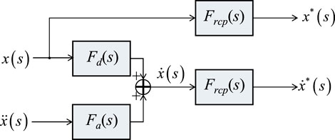
FIGURE 2. Structural response estimation in SPLiTS4ad and minimisation of the central-point shift components.

2.2.2 Response estimation for SPLiTS4a

SPLiTS4a relies only on the measured acceleration and other structural responses (velocity and displacement) must be estimated by integrals of the acceleration. However, the integrals generate unwanted distortions in the displacement and velocity data due to noise within the measured data.

In this regard, SPLiTS is effective as it minimises all the components of central-point shifts, which include the distortion generated at the integrals and residual deformation observed in a severely damaged structure. This feature allows us to minimise these components without separating the residual deformation and distortion derived from the noise. Note that the new form relinquishes estimating the residual deformation in structures, indicating the necessity of other approaches (e.g., onsite visual inspections) to inspect the deformation when it is required.

The distortion caused by noise is much more significant than the residual deformation in structural responses and must be mitigated by a more efficient technique than the filter used for the residual deformation in Eq. 10. The severity of the distortion was more clearly observed in the time domain than in the frequency domain. Thus, this study employs a technique using a moving-average filter that smooths a signal in the time domain to effectively extract the distortion in the integrated data. The filtering technique is shown in Figure 3A, and the structural responses required for TDI are obtained using the procedure shown in Figure 3B.

FIGURE 3

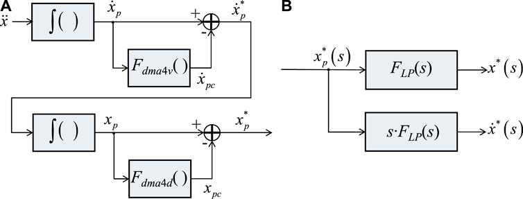
FIGURE 3. Structural response estimation in SPLiTS4a: (A) minimisation of central-point shift components by two-pass moving-average filters, F_dma4v and F_dma4d, which correspond to Eqs 12, 14, respectively, and (B) Structural responses generated by displacement data with the minimised central-point shift component.

The performance of a moving-average filter depends on its average duration, which governs the target frequency to be minimised. When the filter with the averaging duration T_a is employed for a signal with the entire duration T_L, this filter becomes a rectangular pulse, as shown in Figure 4A. According to a study on moving-average filters by Smith (1997), the frequency response in the range of 0.0–0.5 Hz can be described by:

$F_{av}\left(f_a\right)=\frac{\sin \left(\pi \cdot f_a\cdot T_a\right)}{T_a\sin \left(\pi \cdot f_a\right)},(11)$

where f_a = df, 2df, ∙∙∙, 0.5; and df = 1/T_L. Note that Eq. 11 when f_a = 0 was set to F_av (0) = 1 to prevent division by zero.

FIGURE 4

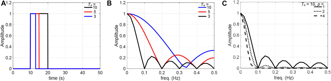
FIGURE 4. Moving average filters: (A) average filters in the time domain, (B) frequency response function |F_av (f_a)|, and (C) frequency response functions |F_av (f_a)^p| for the multiple-pass moving average filter with duration T_a = 10.

Figure 4B clarifies the relationship between the average durations and frequency components to be minimised, showing some unwanted humps in the curve. This indicates that the frequency components corresponding to the humps were not fully removed by the average filter. However, they can be mitigated by a multi-pass moving-average filter technique, which applies a filter multiple time. The four-pass filter (p = 4) in Figure 4C does not have humps, and the frequency components over 0.1 Hz can be fully removed by the filter.

This study introduces a four-pass moving-average filtering technique based on the features of moving-average filters. In this technique, a moving-average filter is applied to the velocity data twice, and a similar filter is applied to the displacement data twice to minimise their distortions. The filtering technique and structural response estimation for SPLiTS4a are described below.

The velocity data with the minimised central-point shift components ${\dot{x}}_p^{*}\left(t\right)$ are obtained by:

$\left\{\begin{array}{l}{\dot{x}}_p^{*}\left(t\right)={\dot{x}}_p\left(t\right)-{\dot{x}}_{pc}\left(t\right)\\ {\dot{x}}_p\left(t\right)={\int }_0^t\ddot{x}\left(\tau \right)d\tau \end{array}\right.(12)$

$\mathrm{w}\mathrm{h}\mathrm{e}\mathrm{r}\mathrm{e}\left\{\begin{array}{l}{\dot{x}}_{pc0}\left(t\right)=\frac{1}{T_v}{{\displaystyle \int }}_t^{t+T_v}{\dot{x}}_p\left({\tau }_1\right)d{\tau }_1\\ {\dot{x}}_{pc}\left(t\right)=\frac{1}{T_v}{{\displaystyle \int }}_t^{t+T_v}{\dot{x}}_{pc0}\left({\tau }_2\right)d{\tau }_2\end{array}\right.(13)$

and T_v is the average duration for the two-pass moving-average filter.

After obtaining the velocity ${\dot{x}}_p^{*}\left(t\right)$, the displacement data with the minimised central-point shift component $x_p^{*}\left(t\right)$ is obtained by:

$\left\{\begin{array}{l}{x}_p^{*}\left(t\right)=x_p\left(t\right)-x_{pc}\left(t\right)\\ x_p\left(t\right)={\int }_0^t{\dot{x}}_p^{*}\left(\tau \right)d\tau \end{array}\right.(14)$

$\mathrm{w}\mathrm{h}\mathrm{e}\mathrm{r}\mathrm{e}\left\{\begin{array}{l}{x}_{pc0}\left(t\right)=\frac{1}{T_d}{{\displaystyle \int }}_t^{t+T_d}{x}_p\left({\tau }_1\right)d{\tau }_1\\ x_{pc}\left(t\right)=\frac{1}{T_d}{{\displaystyle \int }}_t^{t+T_d}{x}_{pc0}\left({\tau }_2\right)d{\tau }_2\end{array}\right.(15)$

and T_d is the average duration for the two-pass moving-average filter.

Based on displacement $x_p^{*}\left(t\right)$ in Eq. 14, the set of structural responses $\left\{{\ddot{x}}^{*}\left(t\right),{\dot{x}}^{*}\left(t\right)\right\}$ for SPLiTS4a is created by:

$\left\{\begin{array}{l}{x}^{*}\left(s\right)=F_{LP}\left(s\right)\cdot x_p^{*}\left(s\right)\\ {\dot{x}}^{*}\left(s\right)=s{F}_{LP}\left(s\right)\cdot x_p^{*}\left(s\right)\end{array}\right.(16)$

where F_LP is the low-pass filter used to realise the differentiation in Eq. 16. F_LP is applied to the responses of the displacement and velocity in Eq. 16. Subsequently, these responses are employed for physical parameter estimation.

As explained above, the structural responses in SPLiTS4a are governed by the four-pass moving-average filtering technique. Its effectiveness depends on the average durations, and we introduce a guide to decide the durations. To the process in Eq. 12, the duration T_v for the first trial should be determined by Eq. 11 with the target frequency to be removed. When the obtained ${\dot{x}}_p^{*}\left(t\right)$ still has some distortion, T_v needs to be adjusted to the one that provides velocity with the minimum distortion. Then, based on ${\dot{x}}_p^{*}\left(t\right)$, the displacement $x_p^{*}\left(t\right)$ is calculated by Eq. 14. In the first trial to remove its central-point shift components, T_d should start from a duration equal to or smaller than T_v, because this process further mitigates the distortion remained even after the process on ${\dot{x}}_p^{*}\left(t\right)$. Again, at the following trials, T_d should be adjusted to the one that realises the displacement with the minimum distortion $x_p^{*}\left(t\right)$.

2.3 Structural state indices for condition assessments

The time-varying physical parameters in a nonlinear structure can be equivalently described as the physical parameters of piecewise linearised structures using SPLiTS. The obtained parameters, described in the time history, are good indices for structural condition assessment. Time-history damping allows us to obtain the associated energy (Akiyama 1985), which is referred to as structural energy absorption in this study. This absorption is a useful index for describing seismic structural damage and degradation.

For a structure with the time-varying physical parameters in Eq. 6, the structural energy absorption on the ith storey $E_{ci}\left(t\right)$ is obtained as follows:

$E_{ci}\left(t\right)={\int }_0^t{c}_i\left(\tau \right){\dot{\widehat{x}}}_i{\left(\tau \right)}^{2}d\tau (17)$

Eq. 17 represents the exact energy absorption when the time-varying damping coefficient in Eq. 6 is exactly known, but accurate identification of the time-varying parameters is an extremely difficult task.

We calculate the energy absorption using the physical parameters obtained using SPLiTS and the structural energy absorption based on the time-history damping provided by SPLiTS becomes:

$E_{ci}^{*}\left(t\right)={\int }_0^t{c}_i^{*}\left(\tau \right){\dot{\widehat{x}}}_i^{*}{\left(\tau \right)}^{2}d\tau (18)$

where $E_{ci}^{*}\left(t\right)$ is the structural energy absorption calculated using the estimated ith storey’s damping coefficient.

Furthermore, this study standardises the energy absorption in Eq. 18 by the ith storey’s weight (i.e., m_i∙g, where g is the gravitational acceleration) to make it a standard index for various structures with different weights. The standardised energy absorption, which has the dimensions of displacement, is expressed as:

$E_{cdi}^{*}\left(t\right)=\frac{E_{ci}^{*}\left(t\right)}{m_{i}g}(19)$

where $E_{cdi}^{*}$ denotes the equivalent displacement of the structural energy absorption on the ith storey. The rate of increase in Eq. 19, which has the dimensions of velocity, can be obtained by:

$E_{cvi}^{*}\left(t\right)={\dot{E}}_{cdi}^{*}\left(t\right)(20)$

where $E_{cvi}^{*}$ is the equivalent velocity of the rate of increase in energy absorption on the ith storey.

SPLiTS regards the yielding of structural components as additional structural energy absorption, which appears as an increase in $E_{cdi}^{*}$. In which, excessive increase is believed to fracture some components, which physically means a decrease in constraints within a storey. The occurrence of fractures (i.e., reduction in the constraints) can be deduced by its storey stiffness described in the time history because the storey constraint condition is demonstrated by its stiffness, particularly within the steady-state, in which the structure undergoes free vibrations after a seismic excitation.

Thus, the structural condition assessments in this study focus on the storey stiffness at the steady-state, referred to as steady stiffness, the time-history physical parameters estimated by SPLiTS, the structural energy absorption in Eq. 19, and its rate of increase in Eq. 20. These factors are referred to as structural state indices in this study.

3 Examination of SPLiTS4a

This study examines SPLiTS4a by applying it to structural response data obtained from a series of E-Defense shake table experiments on the structure shown in Figure 5. The experiments are detailed in Section 3.1, and SPLiTS4a is examined using the experimental data in Section 3.2.

FIGURE 5

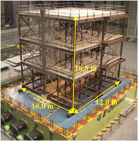
FIGURE 5. Three-storey steel structure tested by E-Defense.

3.1 Shake table experiments at E-defense

Here, we briefly introduce the experimental conditions and results, as well as the modal parameters obtained by the system identification tests.

3.1.1 Experimental conditions

A full-scale three-storey structure in Figure 5 was designed to duplicate a typical steel structure built in Japan in the early 1990s. It consisted of 2-span frames for both longitudinal and transverse directions, and its size was 12.0 m × 10.0 m with a height of 10.8 m. The masses of the first, second, and third storeys were 44.9, 43.9, and 40.6 t, respectively.

In the experiments, servo-accelerometers were placed at five points on each storey (four corners and their centre) as well as the base. Two laser displacement transducers (measurable range: ±250 mm) were placed on the protection stands on each storey to measure each inter-storey drift in the longitudinal direction. The sampling interval was set to dt = 0.001 s.

The structure was uniaxially excited in the longitudinal direction using the two ground acceleration records shown in Figure 6. The one in Figure 6A is the North-South component of the ground acceleration data recorded at the Japan Railway Takatori station during the 1995 Hyougo-ken Nanbu (Kobe) earthquake. The other ground acceleration data in Figure 6A were artificially synthesised at the site of Kobe City Hall for an anticipated Nankai Trough earthquake, which has been a major concern in Japan. These were selected to examine the remaining seismic resistance performance of the structure against the anticipated earthquake, even after it was severely shaken by the Kobe earthquake. These ground motions are referred to as the Takatori and Nankai motions in this study.

FIGURE 6

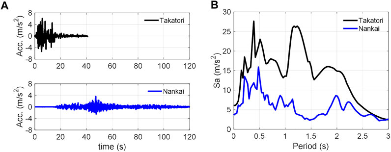
FIGURE 6. Ground motion records employed in the E-Defense experiments: (A) acceleration time history and (B) acceleration response spectra.

According to the response spectra in Figure 6B, the Takatori motion surpasses the Nankai motion over the entire range of ∼3 s. Based on these ground motion characteristics, shake table experiments were performed with the following amplitudes: {40%, 60%, 80%, 100%} for the Takatori motion, and {50%, 100%, 150%} for the Nankai motion.

System identification tests using band-limited white noise were performed before and after each seismic excitation to investigate the modal parameters of the structure. According to the system identification before the first experiment with the Takatori motion, the intact structure was found to have natural frequencies of 1.37, 4.46, and 8.21 Hz.

3.1.2 Structural responses obtained by shake table experiments

The experiments were conducted using the Takatori motion with four amplitude cases {40%, 60%, 80%, 100%} and the Nankai motion with three amplitude cases {50%, 100%, 150%}. The maximum inter-storey drift of the structure obtained by these experiments is summarised in Figure 7. Structural responses in the cases of 60% and 100% Takatori motion and 150% Nakani motion are respectively illustrated in Figures 8–10. The hysteresis shown were obtained using the measured inter-storey drift responses and shear forces, which were calculated by the floor acceleration responses and masses. Note that the structural responses of 40% and 80% Takatori motions have been illustrated in detail in the first study on SPLiTS (Enokida and Kajiwara 2020).

FIGURE 7

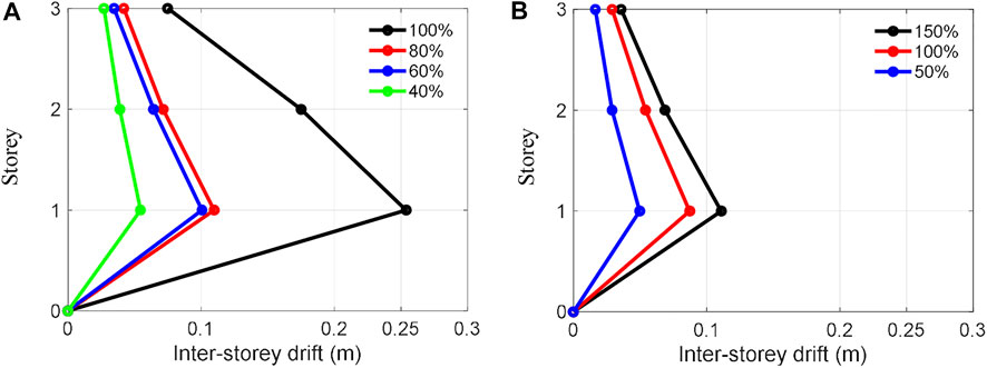
FIGURE 7. Maximum inter-storey drift of the structure excited by (A) Takatori motion and (B) Nankai motion.

FIGURE 8

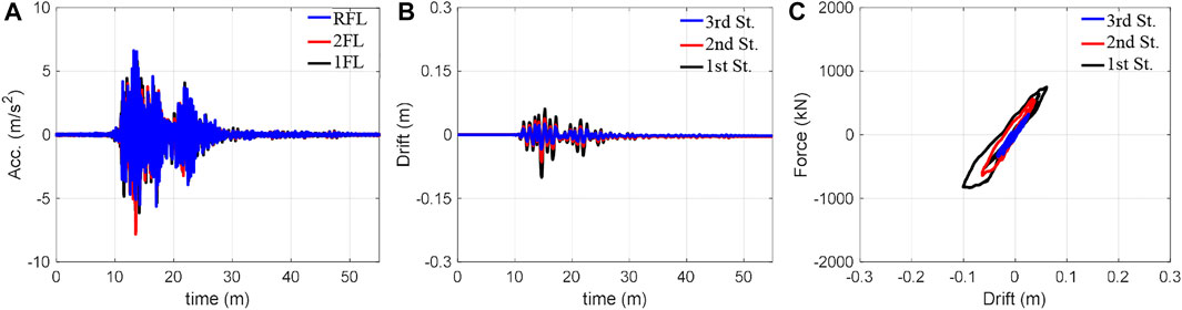
FIGURE 8. Responses of 60% Takatori: (A) acceleration, (B) inter-storey drift, and (C) hysteretic loops.

In the experiments with the Takatori motion, the 40% excitation caused slight yielding in the structural components (Mizushima et al., 2018), and the 60% excitation expanded the yielded areas along with the increase in inter-storey drift on each storey, as seen in Figure 8C. According to Figure 7A, the 80% excitation resulted in a similar inter-storey drift as the 60% excitation. However, 100% excitation resulted in an extremely large inter-storey drift on the first storey that exceeded the measurable range of the displacement transducer: 250 mm. The twisted hysteresis loop of the first storey in Figure 9 is caused by this exceedance.

FIGURE 9

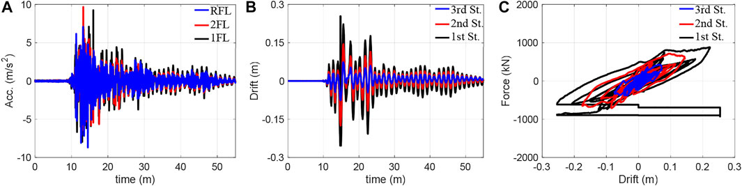
FIGURE 9. Responses of 100% Takatori: (A) acceleration, (B) inter-storey drift, and (C) hysteretic loops.

Experiments with the Nankai motion were performed on the structure, which had already experienced a large deformation by numerous excitations of the Takatori motion. According to Figure 7B, the inter-storey drifts at the excitation of 150% Nankai motion are roughly in between the Takatori motion’s 60% and 80% excitations. Although the inter-storey drifts of 150% Nankai motion in Figure 10B are greater than those of 60% Takatori motion in Figure 8B, the hysteresis loops in Figure 10C are generally not as voluminous as those in Figure 8C.

FIGURE 10

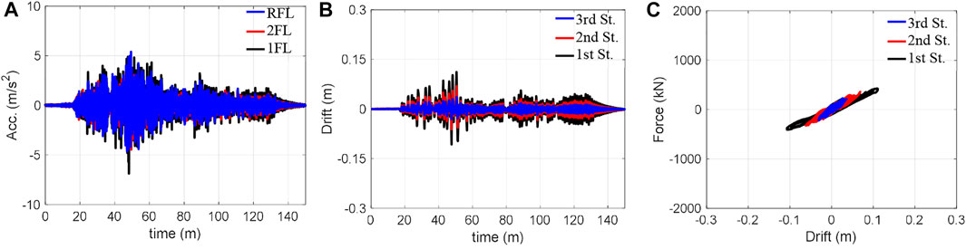
FIGURE 10. Responses of 150% Nankai: (A) acceleration, (B) inter-storey drift, and (C) hysteretic loops.

3.1.3 Modal parameter changes identified by system identification tests

System identification tests were performed with a band-limited white noise after every seismic excitation and the modal parameters of the structure were identified using the FRF method (Ji et al., 2011). Figure 11A illustrates the natural frequencies identified by all the identification tests, and Figure 11B illustrates the modal shapes obtained after the major experiments (80% and 100% Takatori motion as well as 150% Nanaki motion). The modal shapes were standardised, such that the maxima became 1.0.

FIGURE 11

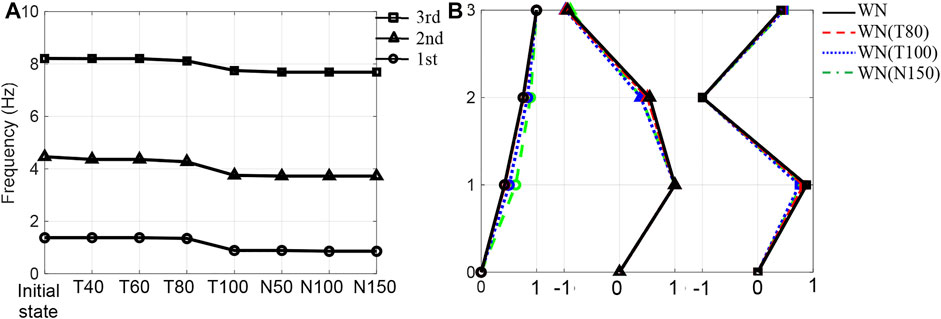
FIGURE 11. Modal parameters obtained by system identification tests after seismic excitations: (A) natural frequencies and (B) Mode shapes identified by a band-limited white noise excitation. Note that WN(T100) is the test using the band limited white noise performed after the seismic excitation of 100% Takatori.

According to Figure 11A, frequency changes are not clearly observed in the identification tests after the Takatori motions of 40%, 60%, and 80%. The 100% values were found to significantly decrease the natural frequencies, indicating the occurrence of severe structural damage. In addition, the decreased natural frequencies remained unchanged with respect to the excitations of the Nankai motion. According to Figure 11B, the modal shapes are not significantly influenced by the Takatori motion for amplitudes up to 80%; however, the modal shapes after 100% differ from those for lower amplitudes. In addition, the first-order modal shape obtained after the 150% Nankai motion also differs from the modal shape after the 100% Takatori motion. This difference is presumably caused by further extensions of structural damage, such as fractures or cracks, by the series of Nankai motion excitations; however, these extensions are not clearly projected into the frequency changes, as shown in Figure 11A.

3.2 Physical parameters estimations by SPLiTS

The new form, SPLiTS4a, was examined in comparison with its original form, SPLiTS4ad, by applying it to the experimental results obtained above.

The parameters required for both forms of SPLiTS were designed to maintain consistency with those used in the first study conducted on SPLiTS (Enokida and Kajiwara 2020). During proper shake table experiments, noise that contaminates the displacement, velocity and acceleration obtained is typically less than 1.0 mm, 10.0 mm/s, and 100 mm/s², respectively. Based on the know-how, the thresholds for the displacement and velocity were set as twice those limits: ε_d = 2.0 mm and ε_v = 20.0 mm/s, respectively. The threshold for the number of steps was set to n₀ = 100 and 300 for the experiments with the Takatori and Nankai motions, respectively, considering their different characteristics.

The filter used in SPLiTS4ad, F_cp(s), was designed by the second order Butterworth low-pass filter with the cut-off frequency of 0.1 Hz and the composite filter in Eq. 10 was designed with ω_c = 1.0∙2π rad/s, which was decided from a reliable range of sensors used in the experiments. The moving-average filtering technique used in SPLiTS4a was designed with T_v = 10.0 s (=10,000∙dt) and T_d = T_v/2 by following the guide in Section 2.2.2. The filter F_LP in Eq. 16 for SPLiTS4a was designed to be the second order low-pass filter with a cut-off frequency of 200 Hz.

3.2.1 Physical parameters obtained from experiments using Takatori motion

Structural state indices were estimated using both SPLiTS forms and the Takatori motion. The results are summarised in Table 2, and the detailed results of the 60% and 100% excitations are illustrated in Figures 12, 13. The steady stiffness listed in Table 2 was obtained based on the rates of increase of the structural energy absorptions, E^*_cv, which can distinguish major structural responses contributing to the absorptions from those that do not.

TABLE 2

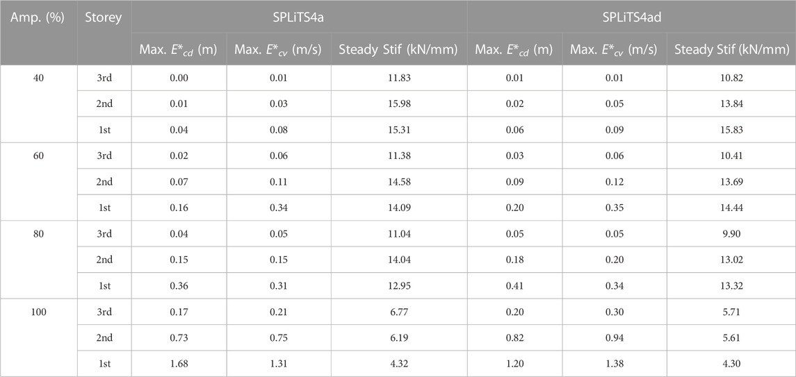
TABLE 2. Structural state indices estimated from the experiments using the Takatori motion.

FIGURE 12

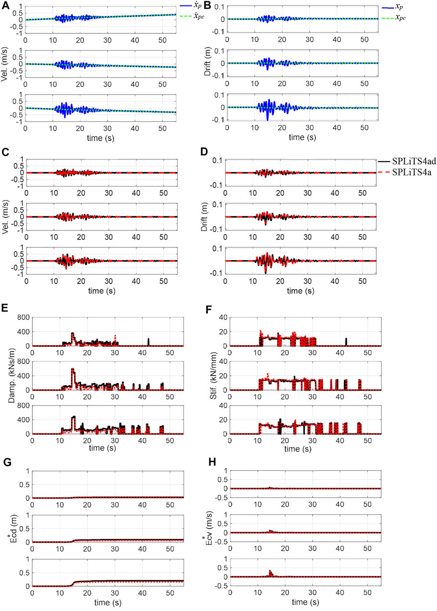
FIGURE 12. Structural responses of 60% Takatori and estimates by SPLiTS: (A) velocity obtained by integration, (B) displacement obtained by integration, (C) velocity with minimised central-point shift components, (D) displacement with minimised central-point shift components, (E) estimated damping, (F) estimated stiffness, (G) structural energy absorption E^*_cd, and (H) energy absorbing rate E^*_cv. N.B.: The top, middle and bottom in each figure corresponds to third, second, and first storeys, respectively.

FIGURE 13

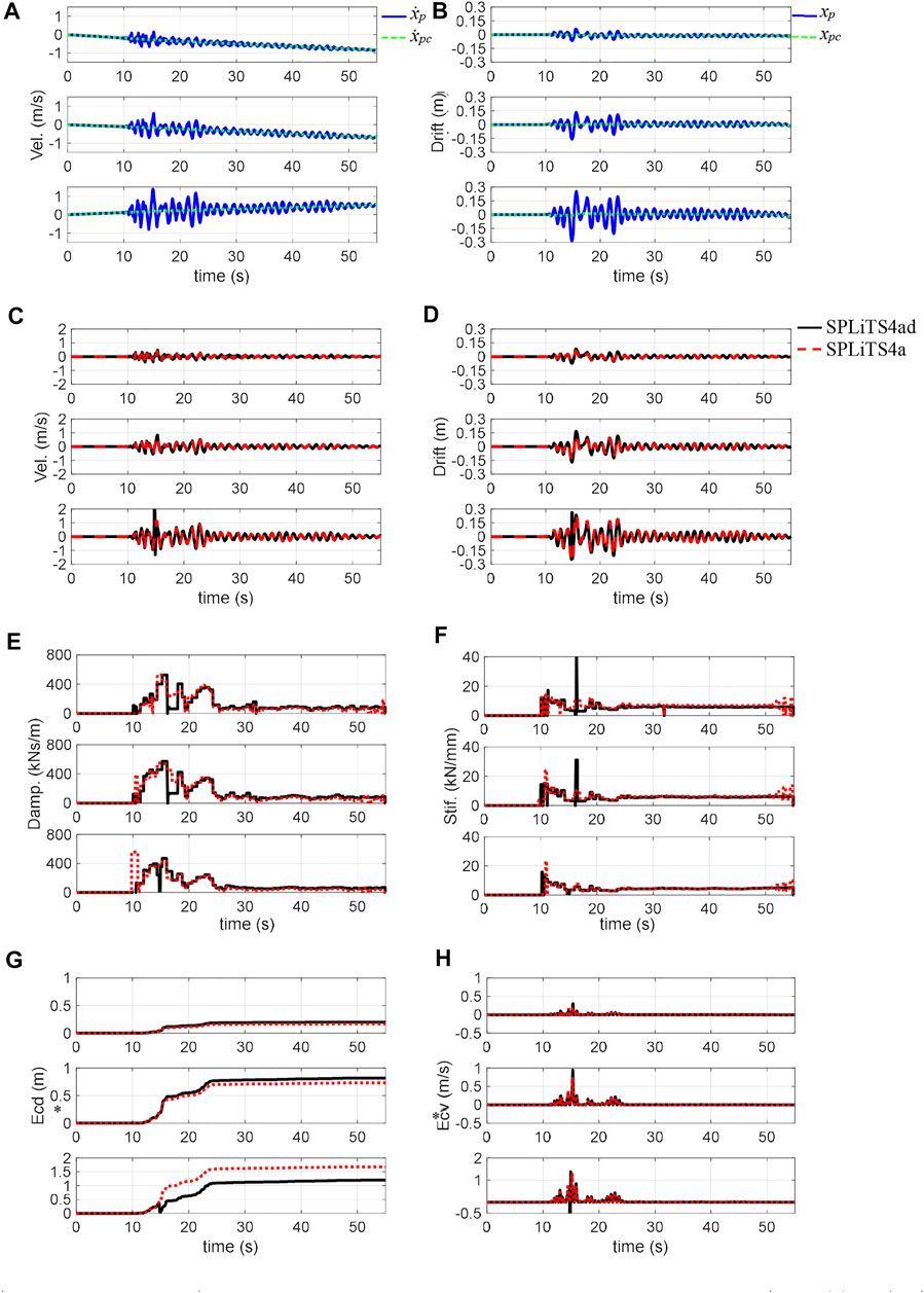
FIGURE 13. Structural responses of 100% Takatori and estimates by SPLiTS: (A) velocity obtained by integration, (B) displacement obtained by integration, (C) velocity with minimised central-point shift components, (D) displacement with minimised central-point shift components, (E) estimated damping, (F) estimated stiffness, (G) structural energy absorption E^*_cd, and (H) energy absorbing rate E^*_cv. N.B.: The top, middle and bottom in each figure corresponds to third, second, and first storeys, respectively.

For the experimental data of the 60% Takatori motion, the four-pass moving-average filtering technique in SPLiT4a effectively extracted the distortion in the displacement and velocity derived from the measured acceleration data, as seen in Figures 12A, B. The displacement and velocity with the minimised central-point shift components by SPLiTS4a in Figures 12C, D are sufficiently close to those obtained by SPLiTS4ad.

Based on the displacement and velocity in Figures 12C, D, the physical parameters for the 60% excitation were estimated, with reasonable similarities between both forms, as shown in Figures 12E, F. In Figure 12G, the structural energy absorptions, E^*_cd, calculated using SPLiTS4a corresponded to that obtained using SPLiTS4ad, although the former is slightly lower. According to Figure 12H, the rates of increase of the absorptions, E^*_cv, are large only in limited ranges, indicating that structural responses out of the ranges do not contribute to energy absorption. Regarding the steady stiffness, which is obtained from the structural responses out of the ranges, the values of SPLiTS4a do not significantly differ from those of SPLiTS4ad, as shown in Table 2.

In the experiment with 100% excitation, the inter-storey drift on the first storey exceeded the measurable range of the displacement transducers. The lack of data in the first storey makes the application of SPLiTS4ad difficult, although SPLiTS4a is not affected by this measurement issue. Figures 13A, B highlights the effectiveness of SPLiTS4a in estimating the velocity and displacement data, whereas Figures 13C, D clarifies the measurement issue for SPLiTS4ad by showing unwanted pulse-like waves for the velocity and displacement data.

Based on the data in Figures 13C, D, the physical parameters and structural energy absorptions during 100% excitation were reasonably estimated by SPLiTS4a, whereas SPLiTS4ad failed to do so, as shown in Figures 13E, F. The influence of the measurement issue becomes apparent from the structural energy absorptions in Figure 13G, which show a sharp drop for SPLiTS4ad in the first storey. In addition, Figure 13H shows SPLiTS4ad’s negative increase rate within the first storey, which theoretically should not occur. This examination clarifies the superiority of SPLiTS4a over SPLiTS4ad.

3.2.2 Physical parameters obtained from experiments using Nankai motion

Structural state indices were estimated using both SPLiTS forms and the Nankai motion. These results are summarised in Table 3, and the detailed results for the 150% excitation are illustrated in Figure 14. The steady stiffness values listed in Table 3 were obtained in the same manner as those in Table 2.

TABLE 3

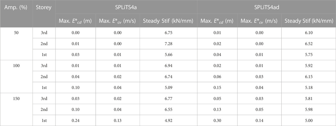
TABLE 3. Structural state indices estimated from the experiments using the Nankai motion.

FIGURE 14

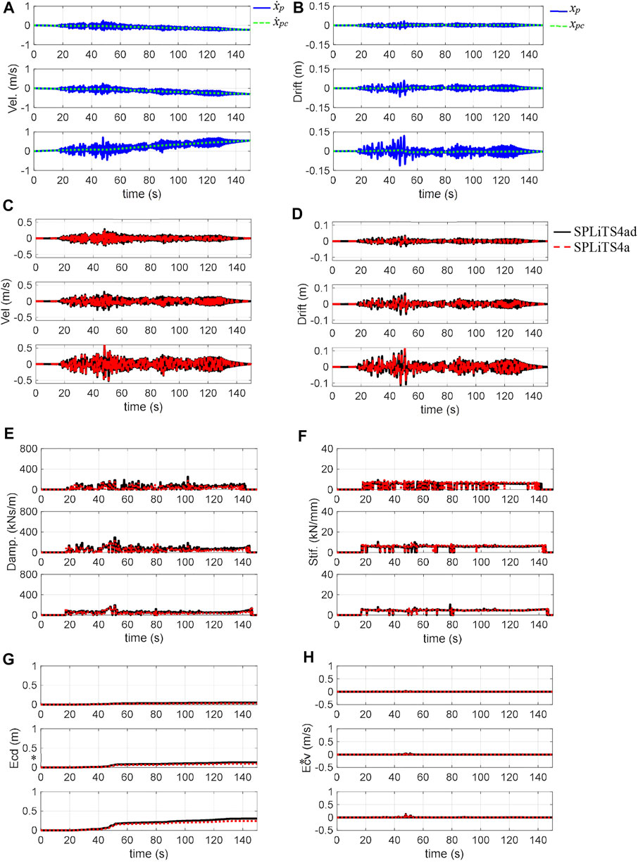
FIGURE 14. Structural responses of 150% Nankai and estimates by SPLiTS: (A) velocity obtained by integration, (B) displacement obtained by integration, (C) velocity with minimised central-point shift components, (D) displacement with minimised central-point shift components, (E) estimated damping, (F) estimated stiffness, (G) structural energy absorption E^*_cd, and (H) energy absorbing rate E^*_cv. N.B.: The top, middle and bottom in each figure corresponds to third, second, and first storeys, respectively.

Figures 14A, B clearly show the effectiveness of the four-pass moving-average filtering technique in the Nankai motion experiments because distortions in the velocity and displacement are effectively extracted by the technique. The response data with the minimised central-point shift components by SPLiTS4a in Figures 14C, D are close to those obtained by SPLiTS4ad.

As shown in Figures 14E, F, the physical parameters estimated by SPLiTS4a are closely matched with those by SPLiTS4ad, although SPLiTS4a′s structural energy absorptions have become slightly lower than that of SPLiTS4ad in Figure 14G. This difference is mainly because of different processes for structural responses of displacement and velocity.

3.2.3 Structural condition assessment based on estimated physical parameters

The physical parameter estimation using both SPLiTS forms provided the structural state indices of the structure (i.e., physical parameters, structural absorptions, and its rates of increase). We discuss the overall results of the estimates by linking them to the structural damage caused by each experiment. Figure 15 summarises the maximum structural energy absorption, steady stiffness, and accumulation of the energy absorption for each storey.

FIGURE 15

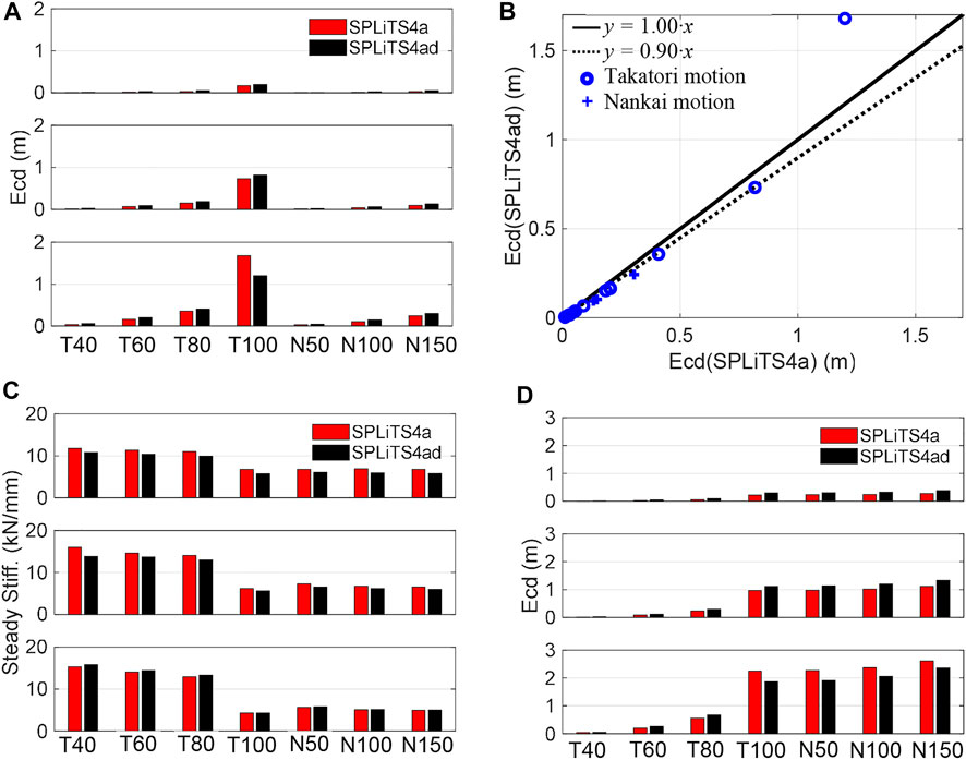
FIGURE 15. Results obtained by SPLiTS4a/ad: (A) maximum structural energy absorption E^*_cd, (B) comparison of E^*_cd, (C) steady stiffness, and (D) accumulation of E^*_cd. N.B.: The top, middle and bottom in each figure corresponds to third, second, and first storeys, respectively.

As shown in Figure 15A, the structural energy absorption increases as the ground motion amplitude becomes larger. In general, the structural energy absorption using SPLiTS4a was 90% of SPLiTS4ad, as shown in Figure 15B, excluding the first storey’s absorption at 100% Takatori motion, which had a displacement measurement issue.

In the case of the Takatori motion, the steady stiffness in Figure 15C gradually decreased with an increase in the structural energy absorption. This indicates that the constraints of the storeys are gradually loosened by the increase in structural energy absorption. The 100% Takatori motion clarifies this feature, showing significant energy absorptions at the first and second storeys in Figure 15A along with significant reductions in steady stiffness at the two storeys in Figure 15C. In fact, during the onsite inspection after the 100% Takatori experiment (Mizushima et al., 2018), the first and second storeys were found to have fractures at the end of the beams. The occurrence of the fractures is more clearly comprehensible from Figure 15D, which shows significant accumulation in these two storeys until the end of the 100% Takatori excitation with significantly lower accumulation in the third storey.

In the case of the Nankai motion, the structural energy absorption is much lower than that of the 100% Takatori motion, as shown in Figure 15A. This resulted in an insignificant increase in the accumulated energy absorptions, as shown in Figure 15D. Thus, the steady stiffness on each storey did not change significantly, as shown in Figure 15C. This result indicates that these excitations caused minimal structural damage. In fact, no additional fractures were found during the onsite inspection after 150% excitation of Nankai motion, although some cracks did extend (Mizushima et al., 2018).

This indicates that the structural energy absorption can quantify the deterioration of a structure caused by numerous seismic excitations. Excessive energy absorption is transformed into fractures of structural components, which can be deduced from the time-history storey stiffness. This examination clarified the effectiveness of the structural state indices obtained by SPLiTS for the condition assessments of seismically damaged structures.

4 Conclusion

This study introduced an acceleration-oriented form of SPLiTS, which does not require displacement measurements. To maintain the simplicity of the original form (i.e., SPLiTS4ad), the new form (i.e., SPLiTS4a) was also based on basic signal processing techniques: integrations of acceleration and a multi-pass moving-average filtering technique. SPLiTS4a uses the integrals of the measured acceleration data to generate its velocity and displacement. Therefore, to effectively minimise the distortions in the integrated data, owing to noise in the measured data, this study incorporated a four-pass moving-average filtering technique. Using these techniques, SPLiTS4a allows us to obtain structural state indices, such as physical parameters of seismically damaged structures, from only measured acceleration data.

This study examined the effectiveness of the new form by applying it to the response data of a three-storey steel structure shaken using two ground acceleration records (i.e., Takatori and Nankai motions) at E-Defense. In the examinations with the Takatori motion, estimates by SPLiTS4a were generally close to those obtained by SPLiTS4ad. In the experiment with 100% Takatori motion, a part of the displacement response was missed because it exceeded the measurable range of displacement transducers. In this case, SPLiTS4a effectively provided structural state indices without any difficulties, whereas SPLiTS4ad failed to do so. In the examinations with the Nankai motion, the structural state indices provided by SPLiTS4a did not greatly differ from those provided by SPLiTS4ad. Thereby, validating the effectiveness of SPLiTS4a.

The structural energy absorption, which is calculated using time-history damping, was shown to be a good index for condition assessments of seismically damaged structures. When the absorption is excessively accumulated within the structure, it leads to fractures in the structural components. Its occurrence was observed based on the time-history storey stiffness. This highlights the importance of monitoring the physical parameters of structures subjected to seismic excitations.

This study illustrated the effectiveness of the new form, SPLiTS4a, to provide physical parameters and structural energy absorptions of seismically damaged structures without measuring the displacement of the structures. The current SPLiTS4a is suitable for structures that can be reasonably modelled by lumped-mass systems and have accelerometers on each storey. To further enhance the practicality of SPLiTS4a, we can study its application to structures where measurement devices are sparsely allocated and other forms of a fishbone model to reflect the flexibility of beams and rotations in structural condition assessments (Nakashima 2002). In addition, we can investigate a systematic method to reasonably determine the parameters required for SPLiTS and automatise its determination to minimise human effort in post-earthquake situations. SPLiTS4a is still based on measuring the acceleration responses on all storeys of structures, and such measurements may be expensive for common buildings such as houses or residential apartments. As advancements of wireless sensors can potentially contribute to cost efficiency, we will investigate the applicability of SPLiTS to acceleration data measured by wireless sensors in the future. In addition, we will study the effectiveness of SPLiTS on a variety of structures (e.g., reinforced concrete, steel, or wood) through various shake table experiments at E-Defense.

Data availability statement

The original contributions presented in the study are included in the article/Supplementary Material, further inquiries can be directed to the corresponding author.

Author contributions

RE and KK contributed to conception and design of the study. RE simulated numerical simulations and wrote the first draft of the manuscript. All authors contributed to manuscript revision, read, and approved the submitted version.

Funding

This study was supported by the research grant (No. 21H01484) from the Japan Society for the Promotion of Science.

Conflict of interest

The authors declare that the research was conducted in the absence of any commercial or financial relationships that could be construed as a potential conflict of interest.

Publisher’s note

All claims expressed in this article are solely those of the authors and do not necessarily represent those of their affiliated organizations, or those of the publisher, the editors and the reviewers. Any product that may be evaluated in this article, or claim that may be made by its manufacturer, is not guaranteed or endorsed by the publisher.

References

Agbabian, M. S., Masri, S. F., Miller, R. K., and Caughey, T. K. (1991). System identification approach to detection of structural changes. Journal of Engineering Mechanics 117, 3702–4390. doi:10.1061/(ASCE)0733-9399(1991)117:2(370)

CrossRef Full Text | Google Scholar

Akiyama, H. (1985). Earthquake-resistant limit-state design for buildings. Tokyo, Japan: University of Tokyo Press.

Google Scholar

Astroza, R., Gutiérrez, G., Repenning, C., and Hernández, F. (2018). Time-variant modal parameters and response behavior of a base-isolated building tested on a shake table. Earthquake Spectra 34, 121–143. doi:10.1193/032817EQS054M

CrossRef Full Text | Google Scholar

Balsamo, L., and Betti, R. (2015). Data-based structural health monitoring using small training data sets. Structural Control and Health Monitoring 22, 1240–1264. doi:10.1002/stc.1744

CrossRef Full Text | Google Scholar

Beskhyroun, S., Oshima, T., and Mikami, S. (2011). Wavelet-based technique for structural damage detection. Structural Control and Health Monitoring 17, 473–494. doi:10.1002/stc.316

CrossRef Full Text | Google Scholar

Brownjohn, J. (2007). Structural health monitoring of civil infrastructure. Philosophical Transactions of the Royal Society A 365, 589–622. doi:10.1098/rsta.2006.1925

PubMed Abstract | CrossRef Full Text | Google Scholar

Carden, E. P., and Mita, A. (2011). Challenges in developing confidence intervals on modal parameters estimated for large civil infrastructure with stochastic subspace identification. Structural Control and Health Monitoring 18, 53–78. doi:10.1002/stc.358

CrossRef Full Text | Google Scholar

Doebling, S. W., Farrar, C. R., Prime, M. B., and Shevitz, D. W. (1996). Damage identification and health monitoring of structural and mechanical systems from changes in their vibration characteristics: A literature review. Washington, DC, USA: Los Alamos National Lab. doi:10.2172/249299

CrossRef Full Text | Google Scholar

Enokida, R., and Kajiwara, K. (2019). Nonlinear signal-based control for single-axis shake tables supporting nonlinear structural systems. Structural Control and Health Monitoring 26, e2376. doi:10.1002/stc.2376

CrossRef Full Text | Google Scholar

Enokida, R., and Kajiwara, K. (2020). Simple piecewise linearisation in time series for time-domain inversion to estimate physical parameters of nonlinear structures. Structural Control and Health Monitoring 27, 1–23. doi:10.1002/stc.2606

CrossRef Full Text | Google Scholar

Enokida, R. (2019). Stability of nonlinear signal-based control for nonlinear structural systems with a pure time delay. Structural Control and Health Monitoring 26, e2365. doi:10.1002/stc.2365

CrossRef Full Text | Google Scholar

Enokida, R., Takewaki, I., and Stoten, D. (2014). A nonlinear signal-based control method and its applications to input identification for nonlinear SIMO problems. Journal of Sound and Vibration 333, 6607–6622. doi:10.1016/j.jsv.2014.07.014

CrossRef Full Text | Google Scholar

Farrar, C. R., and Worden, K. (2006) An introduction to structural health monitoring. Philosophical Transactions of the Royal Society A: Mathematical, Physical and Engineering Sciences 365:303–315. doi:10.1098/rsta.2006.1928

PubMed Abstract | CrossRef Full Text | Google Scholar

Fujino, Y., Siringoringo, D. M., Ikeda, Y., Nagayama, T., and Mizutani, T. (2019). Research and implementations of structural monitoring for bridges and buildings in Japan. Engineering 5, 1093–1119. doi:10.1016/j.eng.2019.09.006

CrossRef Full Text | Google Scholar

Gul, M., and Catbas, F. N. (2011). Structural health monitoring and damage assessment using a novel time series analysis methodology with sensor clustering. Journal of Sound and Vibration 330, 1196–1210. doi:10.1016/j.jsv.2010.09.024

CrossRef Full Text | Google Scholar

Hearn, G., and Testa, R. B. (1991). Modal analysis for damage detection in structures. Journal of Structural Engineering 117, 3042–3063. doi:10.1061/(asce)0733-9445(1991)117:10(3042)

CrossRef Full Text | Google Scholar

Huang, C. S. (2001). Structural identification from ambient vibration measurement using the multivariate AR model. Journal of Sound and Vibration 241, 337–359. doi:10.1006/jsvi.2000.3302

CrossRef Full Text | Google Scholar

Hwang, S-H., and Lignos, D. G. (2018). Assessment of structural damage detection methods for steel structures using full-scale experimental data and nonlinear analysis. Bulletin of Earthquake Engineering 16, 2971–2999. doi:10.1007/s10518-017-0288-2

CrossRef Full Text | Google Scholar

Ikeda, Y. (2016). Verification of system identification utilizing shaking table tests of a full-scale 4-story steel building. Earthquake Engineering and Structural Dynamics 45, 543–562. doi:10.1002/eqe.2670

CrossRef Full Text | Google Scholar

Ji, X., Fenves, G. L., Kajiwara, K., and Nakashima, M. (2011). Seismic damage detection of a full-scale shaking table test structure. Journal of Structural Engineering 137, 14–21. doi:10.1061/(asce)st.1943-541x.0000278

CrossRef Full Text | Google Scholar

Kang, J. S., Park, S. K., Shin, S., and Lee, H. S. (2005). Structural system identification in time domain using measured acceleration. Journal of Sound and Vibration 288, 215–234. doi:10.1016/j.jsv.2005.01.041

CrossRef Full Text | Google Scholar

Katayama, T. (2005). Subspace methods for system identification. London, UK: Springer. doi:10.1007/1-84628-158-X

CrossRef Full Text | Google Scholar

Kim, J., and Lynch, J. P. (2012). Subspace system identification of support excited structures–part II: Gray-box interpretations and damage detection. Earthquake Engineering and Structural Dynamics 41, 2253–2271. doi:10.1002/eqe.2185

CrossRef Full Text | Google Scholar

Kitada, Y. (1998). Identification of nonlinear structural dynamic systems using wavelets. Journal of Engineering Mechanics 124, 105910–111066. doi:10.1061/(asce)0733-9399(1998)124:10(1059)

CrossRef Full Text | Google Scholar

Kuleli, M., and Nagayama, T. (2020). A robust structural parameter estimation method using seismic response measurements. Structural Control and Health Monitoring 27, 1–23. doi:10.1002/stc.2475

CrossRef Full Text | Google Scholar

Ljung, L. (1998). System identification: Theory for the user (prentice Hall information and system sciences series). 2. New York, NY, USA: Prentice Hall.

Google Scholar

Lu, Y., and Gao, F. (2005). A novel time-domain auto-regressive model for structural damage diagnosis. Journal of Sound and Vibration 283, 1031–1049. doi:10.1016/j.jsv.2004.06.030

CrossRef Full Text | Google Scholar

Masri, S. F., Miller, R. K., Saud, A. F., and Caughey, T. K. (1987b). Identification of nonlinear vibrating structures: Part II—applications. Journal of Applied Mechanics 54, 923–929. doi:10.1115/1.3173140

CrossRef Full Text | Google Scholar

Masri, S. F., Miller, R. K., Saud, A. F., and Caughey, T. K. (1987a). Identification of nonlinear vibrating structures: Part I—formulation. Journal of Applied Mechanics 54, 918–922. doi:10.1115/1.3173139

CrossRef Full Text | Google Scholar

Mizushima, Y., Mukai, Y., Namba, H., Taga, K., and Saruwatari, T. (2018). Super-detailed FEM simulations for full-scale steel structure with fatal rupture at joints between members–shaking-table test of full-scale steel frame structure to estimate influence of cumulative damage by multiple strong motion: Part 1. Japan Architectural Review 1, 96–108. doi:10.1002/2475-8876.10016

CrossRef Full Text | Google Scholar

Moaveni, B., and Asgarieh, E. (2012). Deterministic-stochastic subspace identification method for identification of nonlinear structures as time-varying linear systems. Mechanical Systems and Signal Processing 31, 40–55. doi:10.1016/j.ymssp.2012.03.004

CrossRef Full Text | Google Scholar

Nagarajaiah, S., and Basu, B. (2009). Output only modal identification and structural damage detection using time frequency & wavelet techniques. Earthquake Engineering and Engineering Vibration 8, 583–605. doi:10.1007/s11803-009-9120-6

CrossRef Full Text | Google Scholar

Nagarajaiah, S., and Yang, Y. (2017). Modeling and harnessing sparse and low-rank data structure: A new paradigm for structural dynamics, identification, damage detection, and health monitoring. Structural Control and Health Monitoring 24, e1851. doi:10.1002/stc.1851

CrossRef Full Text | Google Scholar

Nair, K. K., Kiremidjian, A. S., and Law, K. H. (2006). Time series-based damage detection and localization algorithm with application to the ASCE benchmark structure. Journal of Sound and Vibration 291, 349–368. doi:10.1016/j.jsv.2005.06.016

CrossRef Full Text | Google Scholar

Nakashima, M. (2002). Generic frame model for simulation of earthquake responses of steel moment frames. Earthquake Engineering and Structural Dynamics 31 (3), 671–692. doi:10.1002/eqe.148

CrossRef Full Text | Google Scholar

Nakashima, M., Nagae, T., Enokida, R., and Kajiwara, K. (2018). Experiences, accomplishments, lessons, and challenges of E-defense–Tests using world’s largest shaking table. Japan Architectural Review 1, 4–17. doi:10.1002/2475-8876.10020

CrossRef Full Text | Google Scholar

Neild, S. A., McFadden, P. D., and Williams, M. S. (2003). A review of time-frequency methods for structural vibration analysis. Engineering Structures 25, 713–728. doi:10.1016/S0141-0296(02)00194-3

CrossRef Full Text | Google Scholar

Ntotsios, E., Papadimitriou, C., Panetsos, P., Karaiskos, G., Perros, K., and Perdikaris, P. C. (2009). Bridge health monitoring system based on vibration measurements. Bulletin of Earthquake Engineering 7, 469–483. doi:10.1007/s10518-008-9067-4

CrossRef Full Text | Google Scholar

Roy, K., Bhattacharya, B., and Ray-Chaudhuri, S. (2015). ARX model-based damage sensitive features for structural damage localization using output-only measurements. Journal of Sound and Vibration 349, 99–122. doi:10.1016/j.jsv.2015.03.038

CrossRef Full Text | Google Scholar

Shintani, K., Yoshitomi, S., and Takewaki, I. (2017). Direct linear system identification method for multistory three-dimensional building structure with general eccentricity. Frontiers in Built Environment 3, 1–8. doi:10.3389/fbuil.2017.00017

CrossRef Full Text | Google Scholar

Shintani, K., Yoshitomi, S., and Takewaki, I. (2020). Model-free identification of hysteretic restoring-force characteristic of multi-plane and multi-story frame model with in-plane flexible floor. Frontiers in Built Environment 6, 1–16. doi:10.3389/fbuil.2020.00048

CrossRef Full Text | Google Scholar

Shokravi, H., Shokravi, H., Bakhary, N., Rahimian Koloor, S. S., and Petru, M. (2020). Health monitoring of civil infrastructures by subspace system identification method: An overview. Applied Sciences 10, 2786. doi:10.3390/app10082786

CrossRef Full Text | Google Scholar

Sivori, D., Cattari, S., and Lepidi, M. (2022). A methodological framework to relate the earthquake-induced frequency reduction to structural damage in masonry buildings. Bulletin of Earthquake Engineering 20, 4603–4638. doi:10.1007/s10518-022-01345-8

CrossRef Full Text | Google Scholar

Smith, S. W. (1997). The scientist and engineer’s guide to digital signal processing. San Diego, CA, USA: California Technical Publishing.

Google Scholar

Sohn, H., Farrar, C. R., Hunter, N. F., and Worden, K. (2001). Structural health monitoring using statistical pattern recognition techniques. Journal of Dynamic Systems, Measurement and Control 123, 706–711. doi:10.1115/1.1410933

CrossRef Full Text | Google Scholar

Stoten, D. P. (2001). Fusion of kinetic data using composite filters. Proceedings of The Institution of Mechanical Engineers, Part I: Journal of Systems and Control Engineering 215, 483–497. doi:10.1177/095965180121500505

CrossRef Full Text | Google Scholar

Tobita, J. (1996). Evaluation of nonstationary damping characteristics of structures under earthquake excitations. Journal of Wind Engineering and Industrial Aerodynamics 59, 283–298. doi:10.1016/0167-6105(96)00012-8

CrossRef Full Text | Google Scholar

Toussi, S., and Yao, J. T. P. (1983). Hysteresis identification of existing structures. Journal of Engineering Mechanics 109, 11895–21202. doi:10.1061/(asce)0733-9399(1983)109:5(1189)

CrossRef Full Text | Google Scholar

Vidal, F., Navarro, M., Aranda, C., and Enomoto, T. (2014). Changes in dynamic characteristics of Lorca RC buildings from pre- and post-earthquake ambient vibration data. Bulletin of Earthquake Engineering 12, 2095–2110. doi:10.1007/s10518-013-9489-5

CrossRef Full Text | Google Scholar

Wu, W-H., Wang, S-W., Chen, C-C., and Lai, G. (2016). Application of stochastic subspace identification for stay cables with an alternative stabilization diagram and hierarchical sifting process. Structural Control and Health Monitoring 23, 1194–1213. doi:10.1002/stc.1836

CrossRef Full Text | Google Scholar

Xiao, H., Bruhns, O. T., Waller, H., and Meyers, A. (2001). An input/output-based procedure for fully evaluating and monitoring dynamic properties of structural systems via a subspace identification method. Journal of Sound and Vibration 246, 601–623. doi:10.1006/jsvi.2001.3650

CrossRef Full Text | Google Scholar

Xie, L., Mita, A., Luo, L., and Feng, M. Q. (2018). Innovative substructure approach to estimating structural parameters of shear structures. Structural Control and Health Monitoring 25, e2139. doi:10.1002/stc.2139

CrossRef Full Text | Google Scholar

Ying, Y., Garrett, J. H., Oppenheim, I. J., Soibelman, L., Harley, J. B., Shi, J., et al. (2013). Toward data-driven structural health monitoring: Application of machine learning and signal processing to damage detection. Journal of Computing in Civil Engineering 27, 667–680. doi:10.1061/(ASCE)CP.1943-5487.0000258

CrossRef Full Text | Google Scholar