Robust optimal damper placement based on robustness index simultaneously considering variation of elastoplastic design criteria and input level

1 Introduction

In the structural design of buildings, it is common practice to evaluate structural safety with respect to design criteria by calculating the maximum response of major structural components such as columns and beams and vibration control components such as oil dampers. These maximum responses are obtained by conducting time history response analysis to design seismic motion with the prescribed material properties and performance. In addition, from the viewpoint of rational design, many examples of structural optimization exist, with seismic response as one of the constraints (Fragiadakis and Papadrakakis, 2008; Kaveh et al., 2010; Gholizadeh, 2015; Papavasileiou and Charmpis, 2016). However, the components of a building may exhibit variations (i.e., uncertainties) in a given performance due to various factors such as construction errors, manufacturing variations, and aging. Since there is a concern that such variations in structural properties may cause the building response beyond the design criteria, it is necessary to understand and adequately account for the influence of the variations on structural performance during structural design.

To investigate the effect of uncertainties in structural properties on the seismic response of buildings, many studies have been conducted on uncertainty analysis methods, including those by Ben-Haim and Elishakoff (1990), Takewaki and Ben-Haim (2005), Henriques et al. (2008), Elishakoff and Ohsaki (2010), and Fujita and Takewaki (2011). One of the purposes of the uncertainty analysis is to find upper and lower bounds of response to parameters with uncertainties, and several efficient methods have been proposed. For example, the interval analysis method is one of the conventional uncertainty analysis methods, in which the uncertain parameters are defined as interval variables with lower and upper bounds. Various interval analysis methods have been proposed (Moens and Vandepitte, 2004; Chen et al., 2009; Moens and Hanss, 2011; Faes and Moens, 2020; Wang et al., 2022). In interval analysis, there is no need to use the probability quantities required for variation based on probability theory since it yields definite upper and lower bounds on the range of the variation of the parameters. Although the interval analysis approach is a classical method, it is easy to handle from a practical standpoint, and it will continue to be used as one of the effective methods to account for uncertainties such as design variables.

Robustness is defined as the resistance or stability of a building performance against various types of uncertainties. In the field of engineering, the keyword “robust design” has been focused on in order to actively consider the variations caused by various uncertainties during design. For example, it has been desired to establish a robust building structure system based on the assumption of variations due to various factors (Doltsinis and Kang, 2004; Lagaros and Papadrakakis, 2007; Gokkaya et al., 2016). Furthermore, optimal design with the consideration of robustness is called robust optimal design. A robust structural optimization design means that there is less degradation of the structural response even in the worst-case variation. As one of the indexes to quantitatively evaluate robustness for optimal design, the robustness function was proposed by Ben-Haim (2006), where variation of uncertainty is assumed.

In recent years, seismic characteristics such as large-amplitude and long-period seismic motions have been clarified, and research on design methods for structures with additive dampers has been intensified (Zhang and Soong, 1992; Castaldo and De luliis 2014; Garivani et al., 2020; Nabid et al., 2020; Xiao et al., 2021). Structural design theory with additive dampers aims to improve damping performance with constraints on cost, worst-case response, and other factors. It is well-known that damper characteristics such as oil dampers may differ between actual and predetermined values due to various uncertainties such as temperature dependence, aging, and manufacturing errors. Fujita and Yasuda (2016) and Fujita et al. (2021) developed robust optimal damper placement problems considering variations in the damping performance of linear and nonlinear oil dampers, but they do not consider building plasticity.

On the other hand, it is important to consider not only the variation in structural properties but also the variation in inputs. Akehashi and Takewaki (2019) developed the optimal placement problem of oil dampers for a critical double impulse (DI) input for an elastoplastic multi-mass model. Critical DI is an input consisting of two impulses that simulate near-fault earthquake motion, and the upper limit of the displacement response can be obtained by acting on the second impulse at the most critical timing for the building. The upper limit of the acceleration response, as well as the displacement response, can be evaluated by back-substituting the critical DI to an equivalent one-cycle sine wave. When considering input variability, the critical DI is also useful in robust optimal design problems because it provides an upper limit of response for a given velocity amplitude $V$ (Fujita et al., 2021).

This paper proposes a new method to evaluate the robustness of elastoplastic buildings concerning uncertain damping coefficients of dampers, considering various variations across a wide range of input levels and performance criteria. The uncertain design variables are the damping coefficients of the oil damper added to the building. Compared to the previous study conducted by Fujita et al. (2021), this paper focuses on the influence of the input level variation on structural performance including elastoplastic behavior. In the proposed robustness index, the robustness function is extended to consider simultaneous variations in input levels and multiple design criteria. This new robustness index can be derived as a three-dimensional surface. This three-dimensional robustness index can comprehensively evaluate the relationship between the input level of the worst-case resonant seismic motion for buildings and the upper bound of structural responses, such as ductility ratio and floor acceleration. The input excitation is determined as an equivalent one-cycle sine wave according to the critical double impulse theory under the variation in the damping coefficient of the oil damper. By comprehensively and efficiently evaluating that, the risk of performance variability can be considered in more detail in the design. Furthermore, based on the proposed robustness index, a robust optimal design problem is presented to obtain the optimal damper placement while considering uncertainties and robustness evaluation under a wide range of input variations and corresponding performance criteria.

2 Critical double impulse and equivalent one-cycle sine wave

2.1 Critical double impulse

The fling-step seismic motion is known to be observed near surface fault raptures (Hisada and Tanaka, 2021). It is noted that the fling-step seismic motion is a pulsating seismic motion, and the waveform with the largest amplitude is similar to the sinusoidal shape. This kind of pulse-like seismic motions can also be extracted in the Pacific Earthquake Engineering Research Center (PEER) database, one of the world’s most famous seismic databases. Furthermore, long-period pulses, where the predominant period is approximately 3 s, were observed in the Kumamoto earthquake in 2016, and it is important to examine the safety of buildings against such pulsating seismic motions. In order to discuss the response characteristic of the building subjected to such pulse-like ground motion, Kojima and Takewaki (2015, 2016) proposed a method to approximate the one-cycle sine wave by composing a DI input, which is expressed as

${\ddot{u}}_g\left(t\right)=V\delta \left(t\right)-V\delta \left(t-t_0\right),(1)$

where $\delta \left(t\right)$ is the Dirac delta function, $V$ is the input velocity amplitude, and $t_0$ is the impulse time interval. DI is unique, and the characteristics of the input seismic motion can be represented only by $V$ and $t_0$. Assuming the amplitude and period of the one-cycle sine wave to be $A_p$ and ${\omega }_p$, respectively, the equivalent DI velocity amplitude $V_e$ and time interval $t_{0e}$, where the maximum elastoplastic displacement response to the one-cycle sine wave coincides, can be expressed as

$V_e=\frac{{\pi }^2}{{\omega }_p}{f}_{\max }{A}_p\simeq 1.637\frac{A_p}{{\omega }_p},t_{0e}=\frac{\pi }{{\omega }_p}.(2)$

In Eq. 2, $f_{\max }$ was determined so that the maximum values of the acceleration Fourier amplitude spectra of the one-cycle sine wave and DI are the same, i.e., the solution of $f_{\max }$ is the maximum amplitude value of $\left.\sin \left(\omega t_0\right)/{\left({\pi }^2-\left(\omega t_0\right)\right.}^2\right)$. From Eq. 2, given $V$ and $t_0$ of DI, it is possible to find the equivalent one-cycle sine wave acceleration amplitude and period. The relationship between ground acceleration, ground velocity, and ground displacement in double impulse and one-cycle sine wave is shown in Figure 1.

FIGURE 1

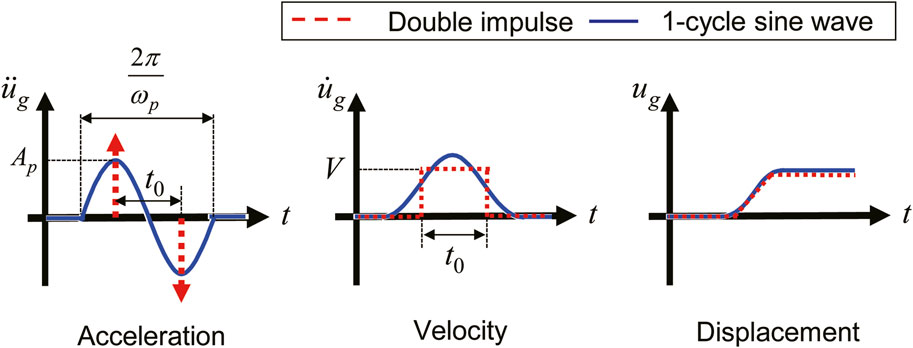
FIGURE 1. Relationship of the time–history of acceleration, velocity, and displacement between double impulse and the one-cycle sine wave.

Basically, since velocity amplitude $V$ is positively correlated with the increasing response, the response characteristics of a building to a double impulse input are focused on the difference in its time interval. When impulse time interval $t_0$ is varied under constant $V$, the maximum inter-story displacement of the building increases or decreases depending on the relationship between the dynamic properties of building and $t_0$. This is because the kinetic energy immediately after the input of the second impulse depends on the velocity response at that moment. The critical input timing $t_0^c$ is defined as the input interval to maximize the structural response. Akehashi and Takewaki (2019) showed that for multi-story buildings, $t_0^c$ is the timing at which the story shear force in the first story becomes zero after the first impulse action. In this paper, we refer to such an input as a critical DI, which can always be regarded as a resonant input. Since it deals with upper bounds on the response to input variation, it allows for a simplified consideration of uncertainty with respect to the input. The input velocity amplitude of the critical DI is denoted as $V_{DI}$ in this paper. Since $t_0^c$ is determined by the hysteresis characteristics of the building and the input velocity amplitude $V_{DI}$, the independent variable for the critical DI is only $V_{DI}$. In this paper, the lower bound of $V_{DI}$ is approximately 0.7 [m/s], and the upper bound of $V_{DI}$ is 1.5 [m/s]. This is determined so that the objective building plasticizes at approximately $V_{DI}=0.7\left[\mathrm{m}/\mathrm{s}\right]$. This means that $V_{DI}=0.7\left[\mathrm{m}/\mathrm{s}\right]$ can be regarded as the elastic limit. On the other hand, $V_{DI}=1.5\left[\mathrm{m}/\mathrm{s}\right]$ is about twice the elastic limit that is corresponding to the life-safety limit level.

2.2 Equivalent one-cycle sine wave

For the response of a building to an impulsive input, from an energetic formulation point of view, kinetic energy is provided to the system at the moment the impulse acts. As one of the ways to take into account such a kinetic energy change in the framework of time history analysis, impulse amplitude $V_{DI}$ of the critical DI can be added to the current velocity of the building at the impulse input timing. However, it is concerning that the acceleration increment also increases locally at the impulse input timing. Therefore, the acceleration response may increase immediately after the impulse input timing, and the maximum acceleration response cannot be properly evaluated. It is well-known that floor acceleration is related to internal damages including building equipment in a building. In order to consider floor accelerations as design criteria for such non-structural damages, the acceleration response must be properly evaluated. In this section, the inverse replacement of the critical DI with a one-cycle sine wave is considered. As shown in Eq. 2, $V$ and $t_0$ can be obtained using $A_p$ and ${\omega }_p$ when replacing the one-cycle sine wave with an equivalent DI. Based on these relations, by finding the critical input timing $t_0^c$ of the second impulse at a certain input velocity amplitude $V$, equivalent one-cycle sine waves $A_p$ and ${\omega }_p$ corresponding to the critical DI are obtained from the inverse of Eq. 2.

By using the one-cycle sine wave equivalent to the critical DI as the input, the input can also be regarded as resonant to the building. This means that the upper limit of the response to input uncertainty can be handled without searching for variations in the input characteristics. Furthermore, one-cycle sine waves are also appropriate for evaluating the maximum acceleration response of the building, because the input waves are continuously and smoothly varied that represent a portion of the actual pulse-like seismic wave. In this paper, the worst input timing $t_0^c$ is first obtained based on the theory of the critical DI by applying time history analysis to the objective building model subjected to a single impulse to search the time when the story shear force is zero, as explained before, and then the equivalent one-cycle sine wave is used as the actual input seismic motion for the structural design. The acceleration amplitude of the equivalent one-cycle sine wave is then dependent on the velocity amplitude $V_{DI}$ of the critical DI.

3 Evaluation of robustness against variations in uncertain parameters

3.1 Definition of the robustness function under varied input levels

Robustness is defined as a measure of the degree of variability of the responses or performance of the structure to various uncertainties derived by input and structural properties. In order to consider robustness during structural design and structural optimization, a quantitative measure of robustness is needed. As one of such quantitative robustness indices of a building against variations in uncertain parameters, Ben-Haim (2006) proposed a robustness function based on the info-gap model. Uncertainty parameters to account for variation can be categorized into probability-based and non-probability-based methods. The info-gap model belongs to the non-probabilistic uncertain model. An interval variable, one of the non-probabilistic uncertainty parameters, is defined as the upper- and lower-limit range of uncertain parameters, defined by the following equation:

${\mathbf{X}}^{\mathrm{I}}\left(\stackrel{\sim }{\mathbf{X}},\alpha \right)=\left\{X_i^{\mathrm{I}}\in \mathbf{R}|X_i^{\mathrm{I}}=\left[{\stackrel{\sim }{X}}_i-\alpha \Delta X_i,{\stackrel{\sim }{X}}_i+\alpha \Delta X_i\right],i=1,2,...,N\right\},(3)$

where ${\left(\right)}^{\mathrm{I}}$ denotes that it is an interval variable or an interval vector. $\Delta X_i$ is the standard variation range of uncertain parameters, and $\alpha$ denotes the degree of variation of the interval variable $X_i^{\mathrm{I}}$. By including $\alpha$ in the interval variable, its upper and lower limits can be made variable. In particular, in the case of $\alpha =0$, Eq. 3 represents a set whose elements are nominal values (design values without considering variation) only.

The concept of the robustness function is shown in Figure 2. The left part of the figure represents the relationship between design variables and structural performance function. As the uncertain design domain represented by variable interval parameters is expanded by uncertainty degree $\alpha$, the region of variation in the building response varies corresponding to $f\left({\mathrm{X}}^{\mathrm{I}}\right)$, as shown in the performance function. On the other hand, the allowable response space should depend on the performance criteria, such as the maximum inter-story drift or top floor acceleration, which are usually used as the design criteria. When the maximum value on the response space due to the variation in design variables coincides with the boundary of the allowable response space, any larger variation will cause a deviation from the allowable response space, and the variation range at this point is the maximum variation range $\widehat{\alpha }$, which is allowed for design purposes. As the maximum allowed range of the variation in design variables depends on the value of the performance criteria $f_c$ required in the design, the robustness function is a representation of these $\widehat{\alpha }-f_c$ relationships.

FIGURE 2

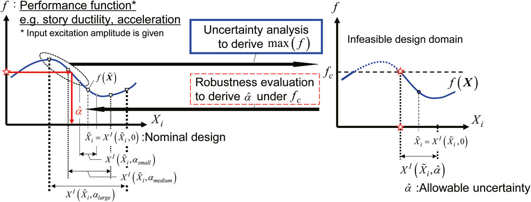
FIGURE 2. Robustness evaluation using uncertainty analysis.

The authors previously proposed optimal design problems using this robustness function, but they conventionally assumed a single variable, such as input levels or performance criteria, and handled the other as a constant (Fujita et al., 2021; Hosoda and Fujita, 2023). However, the amplitude of input external disturbances varies based on the frequency of their occurrence, and it is common practice to set appropriate design criteria for such various input levels, so it is not appropriate to address only specific input levels. Therefore, in this paper, we also focus on changes in the magnitude of the input, i.e., the input velocity amplitude $V_{DI}$. For a constant performance criterion, the robustness function is generally expected to be larger when $V_{DI}$ is smaller. As a function of the nominal value $\stackrel{\sim }{\mathrm{X}}=\left\{{\stackrel{\sim }{X}}_1,{\stackrel{\sim }{X}}_2,...,{\stackrel{\sim }{X}}_N\right\}$ of the design variable assuming variation, the performance criterion $f_c$, and the input velocity amplitude $V_{DI}$, the expanded robustness function is expressed as

$\widehat{\alpha }\left(\stackrel{\sim }{\mathbf{X}},f_c,V_{DI}\right)=\max \left\{\alpha |\max f\left({\mathbf{X}}^{\mathrm{I}}\left(\stackrel{\sim }{\mathbf{X}},\alpha \right),V_{DI}\right)\le f_c\right\},(4)$

where $f$ is the evaluation function for the structural design, such as the maximum inter-story displacement of the building used in the design performance criteria. If $f$ is equal to the required performance $f_c$ at the nominal value, then $\widehat{\alpha }=0$.

3.2 Detailed definition of variables on the robustness function

The robustness function defined in Eq. 4 is a function whose variables are the nominal value $\stackrel{\sim }{\mathrm{X}}$ of the design variable assuming the variation, the performance criterion $f_c$, and the input velocity amplitude $V_{DI}$. This section describes the definitions of these variables in this paper.

3.2.1 Nominal value $\stackrel{\sim }{\mathrm{X}}$ of design variables assuming variation

In this paper, the design variable regarded as the uncertain parameter is the damping coefficient of oil dampers for each story added to the seismic vibration-controlled building, where $\Delta X_i=0.1\times {\stackrel{\sim }{X}}_i$. This means that if the robustness function value $\widehat{\alpha }\left(\stackrel{\sim }{\mathbf{X}},f_c,V_{DI}\right)=1$, the maximum $\pm 10\%$ variation of the design variable will just satisfy the specified performance criteria $f_c$ and $V_{DI}$.

3.2.2 Performance function $f$

The performance function $f$ in Eq. 4 can be set arbitrarily by the structural designer. In the earthquake-resistant structural design, it is important to reduce inter-story displacement, and furthermore, floor acceleration is also an important design index when considering interior damage during an earthquake and habitability for frequently occurring vibrations. In this paper, considering enhancing both structural and non-structural safety of buildings, the multi-performance function is defined as

$f\left(\mathbf{X},V_{DI}\right)=\max \left\{{\mu }_i\left(\mathbf{X},V_{DI}\right)/\overline{\mu },a_{\max ,i}\left(\mathbf{X},V_{DI}\right)/{\overline{a}}_{\max }|i=1,2,...,N\right\},(5)$

where ${\mu }_i$ is the story ductility ratio, which is the ratio of the maximum response displacement to yield displacement in the $i$th story and $a_{\max ,i}$ is the maximum absolute acceleration during the time history in the $i$th story. Since these two structural responses have different dimensions, they are standardized by the design criterion values, which are described below.

3.2.3 Performance criteria $f_c$

Since the performance function in this paper is defined as the standardized multi-objective, as shown in Eq. 5, the performance criteria are given specified coefficients depending on $\overline{\mu }$ and ${\overline{a}}_{\max }$. For example, in the case that the performance criterion $f_c$ is $1.0$, it means that the structural design should not violate the design criteria of ductility on inter-story drift and maximum floor acceleration. In the robustness function discussed in this paper, this performance criterion is handled as a variable to consider the seismic performance redundancy under varied input levels.

3.2.4 Input velocity amplitude $V_{DI}$

The one-cycle sine wave equivalent to the critical DI is used as the actual input seismic motion to the building in this paper. Since the input amplitude of the sine wave is dependent on the critical DI, the input seismic motion can be regarded as the function of the input velocity amplitude $V_{DI}$. By considering the variation in $V_{DI}$, the optimal design problem is handled for various input degrees. It is also possible to implicitly take into account the upper-limit variation of the response to the input variation due to its resonance effect on the structure.

3.3 Application of uncertainty analysis for the evaluation of the robustness function

In order to derive the robustness function defined in Eq. 4, an optimization problem is included that searches for the upper bound on the degree of uncertainty, where the uncertain parameters should be the worst combination to satisfy the specified performance criteria. Although it is difficult to determine the uncertainty bound corresponding to this implied optimization problem, it has been reported that the inverse problem of this optimization problem, i.e., finding the maximum performance function under a given uncertainty bound, can be useful for efficiently deriving the robustness function. This problem can be solved using the uncertainty analysis framework, where the upper and lower bounds of performance functions are derived. A flowchart for evaluating the robustness function in this paper is shown in Figure 3. This flowchart is a minor revision of the previously proposed uncertainty analysis method, called the NURP method. A detailed explanation of this flowchart is described in this section.

FIGURE 3

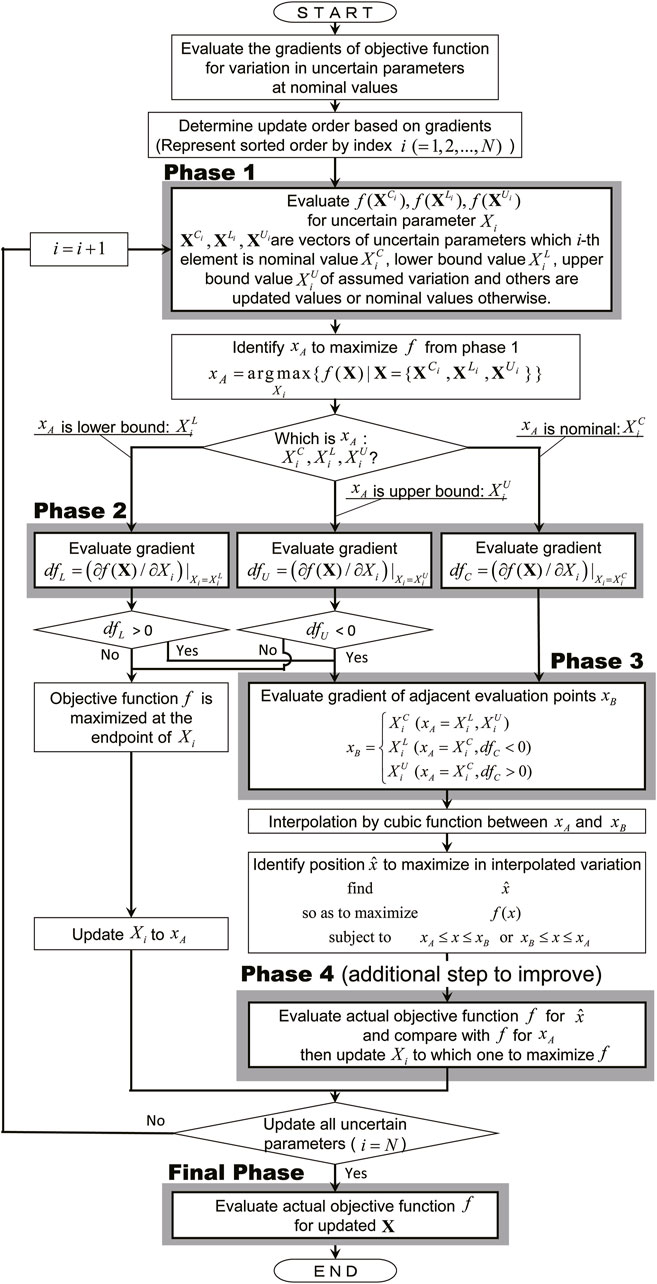
FIGURE 3. Flowchart of the uncertainty analysis method (modified NURP).

First, we consider the case to derive the robustness function of the relationship $\left(\widehat{\alpha },f_c\right)$ for a specific $V_{DI}$. The NURP method proposed by Fujita and Yasuda (2016) is one of the uncertainty analysis methods used to derive the worst combination of uncertain parameters under a given uncertainty degree, where the upper bound of the performance function is obtained. The feature of the NURP method is to approximate the variation in the performance function with a polynomial such as the Taylor series expansion, when only one uncertain parameter is considered to be changed. This approximation is efficient in reducing the computational time for the time-consuming time history response analysis of the building. When the range of variability $\alpha$ is specified, and the obtained upper response limit is regarded as the performance criterion value, specified $\alpha$ corresponds to the robustness function value $\widehat{\alpha }$.

Since the target building should be treated as an elastoplastic building model for various input levels including severe design loadings, it is concerning that there may be an unstable approximation where the performance function changes drastically due to uncertainties. This is mainly because, due to variations, the number of plasticizing stories increase or the maximum response stories for the worst response change. The NURP method uses a cubic function determined by the value of the evaluation point and its neighboring linear gradient when complementing between evaluation points, but if such points exist within the variation interval, a fairly large difference may exist between the critical variation calculated by the NURP method and the actual critical variation.

Therefore, in this paper, as a method to solve this issue without significantly increasing the computational time, we added a procedure to compare the actual response to the critical point calculated by the conventional NURP method with the response to the evaluation points at nominal, upper, and lower bounds of an uncertain parameter (phase 4 in Figure 3). That is, the point with the largest response among the four points is evaluated as the critical point to be updated.

3.4 Robustness function to the simultaneous variation in input levels and performance criteria

Figure 4 shows a conceptual diagram of the $\widehat{\alpha },f_c,V_{DI}$ relationship for a model with a certain nominal value $\stackrel{\sim }{\mathbf{X}}$ for a design variable assuming variation. In this paper, this relationship is referred to as the $\widehat{\alpha }-f_c-V_{DI}$ relationship. Many of the previous studies, e.g., Fujita and Yasuda (2016), Fujita et al. (2021), and Hosoda and Fujita (2023), treated either $f_c,V_{DI}$ as a fixed value and evaluated $\widehat{\alpha }$ as a one-variable function ($\widehat{\alpha }-f_c$ relationship and $\widehat{\alpha }-V_{DI}$ relationship in Figure 4). On the other hand, in this paper, the robustness function $\widehat{\alpha }$ of the model with the specified nominal variable $\stackrel{\sim }{\mathrm{X}}$ is evaluated by considering both variations of $f_c$ and $V_{DI}$. This allows for a comprehensive evaluation of robustness at a wide range of input and performance levels, which has been difficult in previous studies. This expansion of robustness evaluation is expected to be able to evaluate the influence of the variable input amplitude, i.e., multiple design phases such as the elastic limit or life-safety limit, to seismic structural performance.

FIGURE 4

FIGURE 4. Three-dimensional robustness function on input variation and performance criteria.

In order to evaluate the three-dimensional robustness relationship in $\widehat{\alpha }-f_c-V_{DI}$, first, given the input velocity amplitude $V_{DI}$, a few $\left(\widehat{\alpha },f_c\right)$ coordinates were obtained using the uncertainty analysis method, as shown in Section 3.3. Next, the same procedures are performed for various $V_{DI}$, and cubic surfaces are approximately determined once a sufficient number of $\left(\widehat{\alpha },f_c\right)$ coordinates are obtained within the assumed domain of each variable. Note that in this paper, $f_c$ is defined as multi-objective criteria by Eq. 5, and it is difficult to treat single-cubic surfaces for both criteria. Therefore, $\widehat{\alpha }$ with $f_c=\max \left\{{\mu }_i/\overline{\mu }\right\}$ and $\widehat{\alpha }$ with $f_c=\max \left\{a_{\max ,i}/{\overline{a}}_{\max }\right\}$ are separately evaluated as surfaces as described above, and the surface that takes the larger value by comparing two surfaces is selected and integrated to be used as a robustness function with the $\widehat{\alpha }-f_c-V_{DI}$ indicator.

4 Three-dimension robustness function $\widehat{\alpha }$ with performance criteria $f_c$ and input velocity amplitude $V_{DI}$

4.1 Building model and oil damper

This section shows an example of the evaluation of the $\widehat{\alpha }-f_c-V_{DI}$ relationship shown in Section 3, when a one-cycle sine wave equivalent to the critical DI is applied to a shear elastoplastic building model with oil dampers, as shown in Figure 5A. The building model parameters are shown in Table 1. The shear spring is assumed to have bilinear elastoplastic restoring force characteristics, where the stiffness ratio is determined by referring to typical steel structures, and the distribution of the initial shear stiffness is a trapezoidal distribution, where the ratio of the top story to the bottom story is 1:2, and its magnitude is set to match the designed fundamental natural period shown in Table 1 and Figure 5B. The structural damping is assumed to be proportional to the initial stiffness.

FIGURE 5

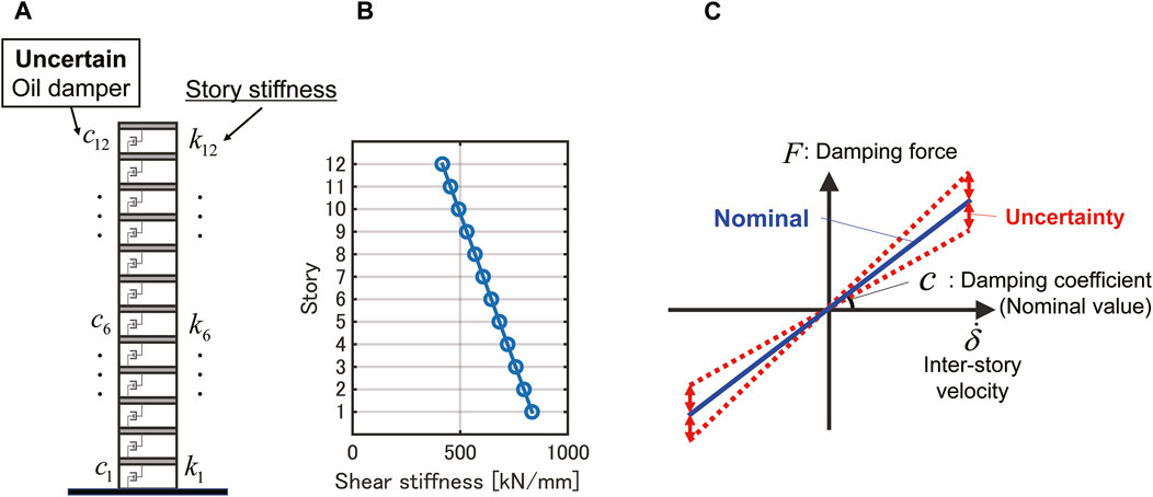
FIGURE 5. Structural properties of the 12 DOF model: (A) elevation, (B) story stiffness distribution, and (C) uncertainty of the damping coefficient.

TABLE1

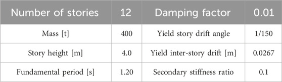
TABLE1. Building model specifications.

The oil damper is assumed to be a linear damper, and in this section, the nominal damping coefficient of the damper at each story is proportional to the story stiffness, so that the added first-order damping factor due to the damper is 0.05. The variation in the damping coefficient is considered the uncertainty of the damping characteristics of the oil damper, as described above (Figure 5C). As a criterion for the range of the variation, we consider a variation of $\pm 10\%$ with respect to the nominal value at $\widehat{\alpha }=1$. The range of variation can be variable according to the robustness function $\widehat{\alpha }$. A time–history analysis for the elastoplastic MDOF model is performed using an originally coded program in MATLAB based on the Newmark $\beta$ method. The accuracy of the time–history response analysis was verified by comparing the results obtained using commercial software.

4.2 An evaluation example of the $\widehat{\alpha }-f_c-V_{DI}$ relationship

Figure 6 shows a three-dimensional robustness function on the $\widehat{\alpha }-f_c-V_{DI}$ relationship obtained by the proposed method in Section 3. Note that since the main focus of this study is to evaluate robustness in the plastic range, the range of input levels where the maximum response displacement of the building model does not exceed the yield displacement is not included in the analysis.

FIGURE 6

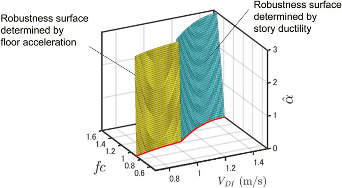
FIGURE 6. Robustness surface based on the multi-objective performance function.

In Figure 6, the $f_c-V_{DI}$ curve for a given $\widehat{\alpha }$ is considered. In this curve, $f_c$ generally increases (worsens) as $V_{DI}$ increases. A design in which the degree of increase in $f_c$ is small even when $V_{DI}$ increases can be a favorable $f_c-V_{DI}$ curve. This is because it implies that the structural performance is high even for the large amplitude of inputs. In addition, for the $\widehat{\alpha }-f_c$ curve at a given $V_{DI}$, $f_c$ generally increases as $\widehat{\alpha }$ increases, i.e., as the variation in the design variable assuming variation increases. A design with a small increase in $f_c$ can be said to be a design with high robustness since the performance deterioration is small even if the variation in the design variables increases. A mentioned above, it is possible to evaluate that a model with a $\widehat{\alpha }-f_c-V_{DI}$ relationship surface, in which the degree of degradation of $f_c$ is small in relation to the increase in $V_{DI}$ in the $f_c-V_{DI}$ curve for each $\widehat{\alpha }$, and $\widehat{\alpha }$ in the $\widehat{\alpha }-f_c$ curve for each $V_{DI}$, has high robustness in a wide range of input levels and performance levels.

Next, to discuss the influence of uncertainties on the obtained $\widehat{\alpha }-f_c-V_{DI}$ relationship diagram, the story direction distribution of the worst variation rate of the damping coefficient, i.e., critical variation of the damping coefficient, that provides the upper limit of the maximum response is shown in Figure 7, and the maximum negative and positive response values corresponding to maximum responses after the first and second impulse action are shown in Figure 8. Both figures show results for some $\widehat{\alpha }$ when $V_{DI}=0.8,1.2,1.5\left[\mathrm{m}/\mathrm{s}\right]$, and horizontal bars in Figure 7 represent the worst-case variation rate of the damping coefficient obtained by the NRUP method.

FIGURE 7

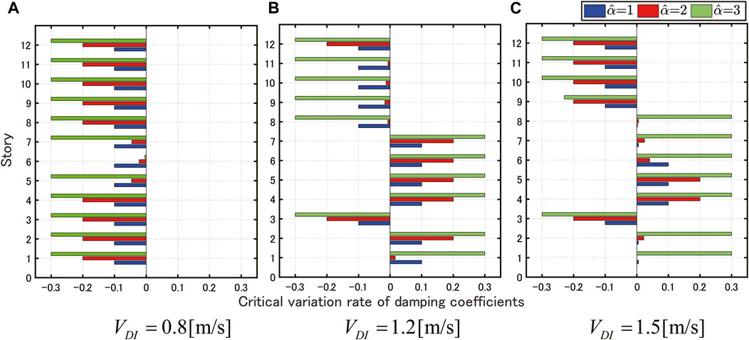
FIGURE 7. Worst combination of damping coefficients for each robustness function value: (A) $V_{DI}=0.8\left[\mathrm{m}/\mathrm{s}\right]$, (B) $V_{DI}=1.2\left[\mathrm{m}/\mathrm{s}\right]$, and (C) $V_{DI}=1.5\left[\mathrm{m}/\mathrm{s}\right]$

FIGURE 8

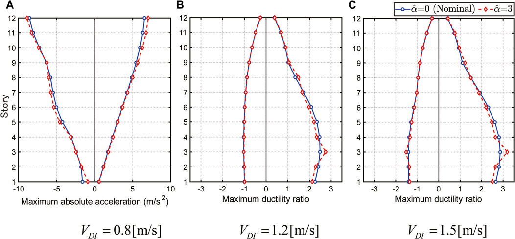
FIGURE 8. Positive and negative maximum performance functions for various input levels: (A) $V_{DI}=0.8\left[\mathrm{m}/\mathrm{s}\right]$, (B) $V_{DI}=1.2\left[\mathrm{m}/\mathrm{s}\right]$, and (C) $V_{DI}=1.5\left[\mathrm{m}/\mathrm{s}\right]$

In the case of $V_{DI}=0.8\left[\mathrm{m}/\mathrm{s}\right]$, the robustness function surface is determined not by the maximum inter-story displacement (maximum story ductility ratio) but by the maximum acceleration response. Around this input level, the maximum response at the negative side is larger than the positive side, and this appears in the top story. The oil dampers treated in this paper are arranged so that the damping is smaller in the upper stories, so the effect of the variation is less pronounced in the upper stories. This is related to the very small slope of the robustness surface to $\widehat{\alpha }$ near this input level. In addition, as shown in Figure 7A, the critical variation distribution of the damping coefficient of the damper is almost the same regardless of $\widehat{\alpha }$ and is at the lower limit for most stories.

On the other hand, in the case of $V_{DI}=1.2\left[\mathrm{m}/\mathrm{s}\right]$, the robustness function surface is given by the maximum story ductility ratio as $f_c$. Since the floor response near the third story, which exhibits the worst-case response, increases locally around this input level, the increase in energy, i.e., the increase in $V_{DI}-\widehat{\alpha }$ required to increase the worst-case response, is relatively small, and the degree of increase in $f_c$ is large relative to the increase in $V_{DI}-\widehat{\alpha }$. Figure 7B and Figure 8B show that the critical variation in the damping coefficient of the damper is at the lower limit in the third story, where the ductility ratio is maximum at the positive side and mostly at the upper limit in the several levels above and below it, regardless of $\widehat{\alpha }$. However, in the other stories (eighth or above), the critical variation is different according to $\widehat{\alpha }$.

In the case of $V_{DI}=1.5\left[\mathrm{m}/\mathrm{s}\right]$, the maximum story ductility ratio is also active for the robustness surface. Figure 8C shows that the maximum inter-story displacement at both negative and positive sides is plasticized in almost stories. In particular, the plasticization at the negative side results in larger energy being absorbed by the hysteresis loop in those stories. Therefore, the increase in energy required to increase the worst-case response near this input level is again larger, and the degree of the increase in $f_c$ is smaller than that in $V_{DI}-\widehat{\alpha }$. As for Figure 7C, it can be shown that the critical variation in damping coefficients of the damper is, as in the case of $V_{DI}=1.2\left[\mathrm{m}/\mathrm{s}\right]$, at the lower limit in the third story, which has the maximum response, and at the upper limit for the fourth and fifth stories immediately above it, regardless of $\widehat{\alpha }$. On the other hand, the lower stories below the third story have different critical variations depending on $\widehat{\alpha }$.

As shown in Figure 7, in the case of the structural design considering the variation in the damping coefficient of the damper, even if a uniform lower limit is adopted, it does not necessarily result in the worst-case response. This investigation and similar results were also discussed by Fujita et al. (2021).

5 Robust optimal design considering uncertainty in damping characteristics of oil dampers

5.1 Optimal design index using robustness functions with performance criteria and input velocity amplitude as variables

In this section, the robust optimal design problem is proposed to determine the oil damper placement that improves the structural performance with robustness using the proposed robustness surface based on the $\widehat{\alpha }-f_c-V_{DI}$ relationship. With regard to robust optimization, many problems have been addressed to optimize robustness at a certain input level or performance criterion, e.g., Fujita and Yasuda (2016), Fujita et al. (2021), and Hosoda and Fujita (2023). However, especially in multi-story high-rise buildings, due to the effects of plasticity and other factors, the variation in the seismic response dependent on various design variables are so complex that it is not possible to properly evaluate the robustness of buildings only at specific input levels or performance criteria. Therefore, in this paper, by using the robustness surface proposed in the previous section that can treat the simultaneous variation in input levels and performance criteria, it is possible to comprehensively evaluate the robustness of the building model with respect to those variations. As for the performance function for the robustness surface, Eq. 5 is also used in this section to consider the multi-objective structural design.

As mentioned in the evaluation example in Section 4, in the $\widehat{\alpha }-f_c-V_{DI}$ relationship, $f_c$ generally increases with respect to increases in $\widehat{\alpha }$ and $V_{DI}$. For a robust optimal design over a wide range of input and performance levels, it is desirable that the degree of increase in $f_c$ on the $\widehat{\alpha }-f_c-V_{DI}$ relationship is small. Therefore, in order to develop the robust optimal problem, we consider evaluating the robustness of a certain building model by the volume $S_{\mathrm{V}}$ of the shaded area, as shown in Figure 9A, where its volume can be calculated by integration by the $\widehat{\alpha }-f_c-V_{DI}$ relationship surface and the plane corresponding to the boundary of each variable. This robustness index used for optimization as the objective function not only allows it to be treated as a scalar value but also improves robustness over a wide range of input and performance levels.

FIGURE 9

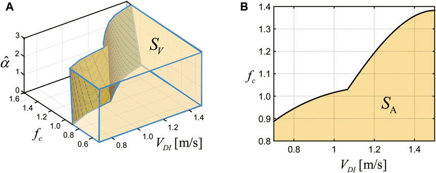
FIGURE 9. Objective function used in optimization problems based on the three-dimensional robustness function: (A) robust optimization problem and (B) normal optimization problem.

5.2 Robust optimal design problem

The robust optimal design problem based on the robustness index presented in Section 5.1 can be expressed as follows:

[Robust optimal design problem]

$\begin{array}{cc}\text{Find}& \stackrel{\sim }{\mathbf{c}}\\ \text{so\hspace{0.5em}as\hspace{0.5em}to\hspace{0.5em}minimize}& S_{\mathrm{V}}\left(\stackrel{\sim }{\mathbf{c}}\right)\\ \text{subject\hspace{0.5em}to}& {\displaystyle \sum }{\stackrel{\sim }{c}}_i\le {\mathrm{c}}_{\text{sum}}\left(\stackrel{\sim }{\mathbf{c}}=\left\{\stackrel{\sim }{c}\right\}\right)\end{array},(6)$

where $\stackrel{\sim }{\mathbf{c}}$ is the nominal value of the damping coefficient of the oil damper (design variable vector) for each story. In general, the higher the damping coefficient of the oil damper, the higher the damping performance, so the upper limit is ${\mathrm{c}}_{\text{sum}}$ as a total constraint to compare robustness under a constant sum of them. The upper limit of the sum of damping coefficients ${\mathrm{c}}_{\text{sum}}$ can be arbitrarily defined. The objective function $S_{\mathrm{V}}\left(\stackrel{\sim }{\mathbf{c}}\right)$ is the volume of the area bounded by the $\widehat{\alpha }-f_c-V_{DI}$ relational surface shown in Section 5.1. This volume $S_{\mathrm{V}}\left(\stackrel{\sim }{\mathbf{c}}\right)$ is expressed by the following equation:

$S_{\mathrm{V}}\left(\stackrel{\sim }{\mathbf{c}}\right)={\int }_{{\underset{\_}{V}}_{DI}}^{{\overline{V}}_{DI}}{\int }_{f_c\left(\underset{\_}{\widehat{\alpha }}\right)}^{f_c\left(\overline{\widehat{\alpha }}\right)}\widehat{\alpha }\left(\stackrel{\sim }{\mathbf{c}}\right)d{f}_{c}d{V}_{DI},(7)$

where ${\overline{V}}_{DI},{\underset{\_}{V}}_{DI},\overline{\widehat{\alpha }},\underset{\_}{\widehat{\alpha }}$ represent the upper and lower bounds of the input level and the interval of the robustness function, respectively, which can be set arbitrarily. This problem is an optimal problem to find the unknown parameters that minimize $S_{\mathrm{V}}\left(\stackrel{\sim }{\mathbf{c}}\right)$. Here, the fmincon function of the MATLAB Optimization Toolbox is applied as the solver for the optimization problem. This solver is a nonlinear programming solver that finds the minimum value of a constrained nonlinear multivariable function, and then it can find parameters that minimize a nonlinear function represented by a vector of unknown parameters. The optimization algorithm for the fmincon function based on the interior point method is used.

5.3 Optimal design problem without considering uncertainties

The robust optimal design problem presented in Section 5.2 aims to suppress the performance deterioration considering variations in the design variables by taking robustness into account. On the other hand, robust optimization may result in a smaller performance value when variation is not considered (at $\widehat{\alpha }=0$). Therefore, we treat the following optimal design problem that cannot consider the variation of uncertainties of structural parameters.

[Normal optimal design problem]

$\begin{array}{cc}\text{Find}& \stackrel{\sim }{\mathbf{c}}\\ \text{so\hspace{0.5em}as\hspace{0.5em}to\hspace{0.5em}minimize}& S_{\mathrm{A}}\left(\stackrel{\sim }{\mathbf{c}}\right)\\ \text{subject\hspace{0.5em}to}& {\displaystyle \sum }{\stackrel{\sim }{c}}_i\le {\mathrm{c}}_{\text{sum}}\left(\stackrel{\sim }{\mathbf{c}}=\left\{\stackrel{\sim }{c}\right\}\right)\end{array}.(8)$

In this paper, the design problem in Eq. 8 is referred to as a “normal optimal design problem.” In order to optimize structural performance for various input levels, an objective function is set up with the intention of obtaining response values to the nominal values for each input level. This objective function is based on ideas similar to those treated in the robust optimization problem, as shown in Eq. 6. The objective function $S_{\mathrm{A}}\left(\stackrel{\sim }{\mathbf{c}}\right)$ is the area obtained from the $f_c-V_{DI}$ relationship in $\widehat{\alpha }=0$, as shown in Figure 9B. This area value can be calculated by integration with respect to the input velocity amplitude as

$S_{\mathrm{A}}\left(\stackrel{\sim }{\mathbf{c}}\right)={\int }_{{\underset{\_}{V}}_{DI}}^{{\overline{V}}_{DI}}{f}_{c}d{V}_{DI}.(9)$

In this problem, the optimal design is to improve the performance at various input levels without considering the variation in the damping coefficient of the oil damper.

5.4 Results and discussion of the robust optimal design

In this section, the results of the robust optimal design problem for finding the optimal damper placement added to the elastoplastic 12-story shear degree of freedoms model treated in Section 4 are shown, and the difference from the normal optimal design is discussed. In the figure legend and following discussions, the mass system model treated in Section 4 is referred to as the “standard model,” the model with dampers where Eq. 8 is applied as the “normal optimization model,” and the model with dampers where Eq. 6 is applied as the “robust optimization model.” The total amount of damping coefficients of the damper ${\mathrm{c}}_{\text{sum}}$ in Eq. 6 and Eq. 8 is the amount corresponding to a damping constant of 5%, as in the standard model. Since the optimization solver, i.e., fmincon, requires an initial solution as the damper placement, the initial solution for deriving the normal optimization model is the standard model and for deriving the robust optimization model is the normal optimization model. The dependence of the fmincon function on the initial solution is discussed later.

As a result of the optimal design problem, the damping coefficient distributions of the oil damper for each model are shown in Figure 10. In addition, for each model, the values of $S_{\mathrm{V}}$ and $S_{\mathrm{A}}$ defined in Eqs 7 and 9, respectively, are shown in Table 2.

FIGURE 10

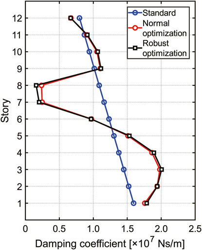
FIGURE 10. Damping coefficient distribution.

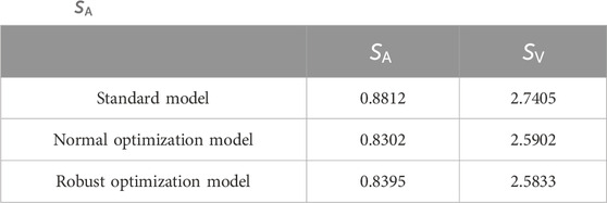
TABLE 2

TABLE 2. ${\mathsf{S}}_{\mathrm{A}}$ and ${\mathsf{S}}_{\mathrm{V}}$ of each model.

Comparing the values of $S_{\mathrm{A}}$ and $S_{\mathrm{V}}$, the standard model is the largest (worst). In addition, the model with the smallest (optimal) value of $S_{\mathrm{A}}$ is the normal optimization model, and $S_{\mathrm{V}}$ is the robust optimization model. This indicates that when comparing the $\widehat{\alpha }-f_c-V_{DI}$ relationship between the normal optimization model and the robust optimization model, the former is superior in the $f_c-V_{DI}$ relationship at $\widehat{\alpha }=0$, but as $\widehat{\alpha }$ increases, the superiority of these different optimization problems changes. In other words, the robust optimization model is superior to the normal optimization model for the variation in the damping coefficients of the oil damper. These are shown in Figure 11, where the $f_c-V_{DI}$ relationship of each model at each $\widehat{\alpha }$ is evaluated.

FIGURE 11

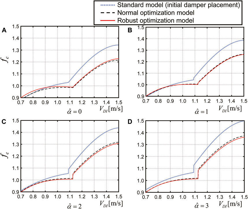
FIGURE 11. Three-dimensional robustness function for various robustness degrees: (A) $\widehat{\alpha }=0$, (B) $\widehat{\alpha }=1$, (C) $\widehat{\alpha }=2$, and (D) $\widehat{\alpha }=3$

From Figure 10, in the robust optimization model, it can be observed that more dampers are placed in the lower and upper stories, and fewer dampers are placed in the middle stories, especially in seventh and eighth stories. This is because, under a constant total damping coefficient of the damper, the response increase can be suppressed even if the damping coefficient varies, by placing more dampers in and around the stories, where the response displacement or acceleration increases due to variations in the damping coefficient. The normal optimization model has a similar placement to the robust optimization model, but the amount of dampers is approximately 22% and 49% larger for the seventh and eighth stories, respectively. It may be pointed out that there is not much difference between the damper placement of the normal and robust optimization models, but it is important to note that the normal optimal design, which is used as a comparison in this paper, takes into account the variability in input levels. It can be said that the normal optimization model has a certain degree of high robustness. Although the damping coefficient difference between both models is small, Table 2 shows that it is possible to improve the $S_{\mathrm{V}}$ value using the proposed robust optimization considering the variation in the structural properties. In addition, obvious differences exist between the distributions of the maximum response in both models, i.e., the worst response occurs at different stories. It indicates that even if there is not much difference in the both nominal values, the influence of that variation on the response is not small.

In order to compare the characteristics of each model, the distributions of the maximum response at a given input level $V_{DI}=0.8,1.2,1.5\left[\mathrm{m}/\mathrm{s}\right]$ is compared at $\widehat{\alpha }=0,1.0,3.0$, as shown in Figure 12.

FIGURE 12

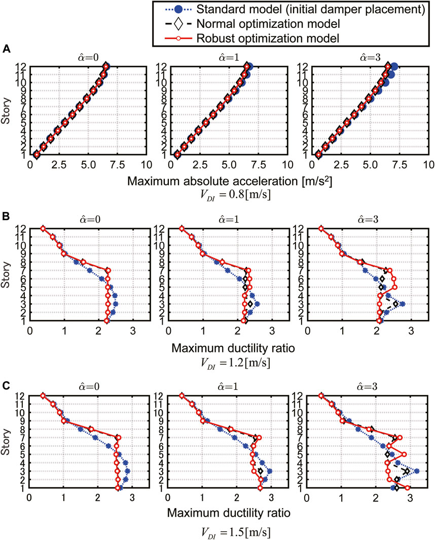
FIGURE 12. Comparison of performance functions for various input levels and robustness degree $\widehat{\alpha }$ = 0, 1, and 3. : (A) V_DI = 0.8 [m/s], (B) V_DI = 1.2 [m/s], and (C) V_DI = 1.5 [m/s].

Figure 12A shows the case of $V_{DI}=0.8\left[\mathrm{m}/\mathrm{s}\right]$. The maximum response acceleration is used as $f_c$ around this input velocity amplitude, and the worst response appears at the top story for any model, input level, and magnitude of variation. It is well-known that the absolute acceleration is often maximized at the top floor in such a high-rise building. In addition, each of the optimization models at $\widehat{\alpha }=3.0$ showed improved performance compared to the standard model. For the other $\widehat{\alpha }$, no significant difference exists between the models.

Figure 12B shows the case of $V_{DI}=1.2\left[\mathrm{m}/\mathrm{s}\right]$. Around this input velocity amplitude, the maximum ductility ratio is predominant as $f_c$, and the location of stories that have the worst response is different for each. Here, as $\widehat{\alpha }$ increases, deformation is concentrated on a specific story, i.e., third story, in the standard model and the normal optimization model. In contrast, there is no such tendency in the robust optimization model, and the middle and lower stories are relatively equally degraded. This indicates that the robust optimization design is highly robust to damper damping variations around this input level and suppresses the concentration of the inter-story drift at a particular floor.

Figure 12C shows the case of $V_{DI}=1.5\left[\mathrm{m}/\mathrm{s}\right]$. Around this input velocity amplitude, the maximum ductility ratio is also selected as $f_c$, and the distribution of the worst response is generally similar to the case of $V_{DI}=1.2\left[\mathrm{m}/\mathrm{s}\right]$, but the deformation in the first story in the robust optimization model at $\widehat{\alpha }=3$ is a little large. Since the objective of robust optimization is to control the inter-story displacement so that it is not excessive in a particular story, this result leaves room for improvement.

As a common feature observed in both the cases of $V_{DI}=1.2,1.5\left[\mathrm{m}/\mathrm{s}\right]$, when $\widehat{\alpha }$ is small, no significant difference exists between the response of the normal and robust optimization models, but as $\widehat{\alpha }$ increases, the distribution of the response becomes significantly different. This is thought to be due to the fact that the response distributions are similar when little variation in damper damping is considered, because no significant difference exists in the nominal damper placement of both models, but when the large variation is considered, a significant difference exists in the critical variation of damping coefficients of the damper.

The performance difference between each model is not so significant when $V_{DI}$ is relatively small, but as $V_{DI}$ increases, the performance difference between the standard model and both optimization models becomes more pronounced. This may be due to the fact that, as a set of performance criteria in this example problem, the maximum ductility ratio adopted as $f_c$ when $V_{DI}$ is large tends to be larger than the maximum response acceleration adopted as $f_c$ when $V_{DI}$ is small after being standardized, so that a damper placement that reduces the maximum ductility ratio was selected as a better solution in the optimization process.

Since it is known that the initial solution dependence in gradient-based optimization like the interior point method in fmincon, several optimization results based on different initial solutions in fmincon are compared in the proposed optimization problems. The optimization solver fmincon function uses the sensitivity of the objective function to successively update the solution until the objective function converges within a specified error range. Therefore, if an inappropriate initial solution is given, the obtained solution may be a local solution or the number of computational iterations required until the objective function converges may be very large. Furthermore, in the example problem, the computational load required to evaluate the objective function $S_{\mathrm{V}}\left(\stackrel{\sim }{\mathrm{c}}\right)$ in Eq. 7 of the robust optimal design problem is relatively large. In contrast, the evaluation of $S_{\mathrm{A}}\left(\stackrel{\sim }{\mathrm{c}}\right)$ in Eq. 9, the objective function of the normal optimal design problem, is not so difficult. For example, the number of time history response analyses performed to calculate $S_{\mathrm{A}}\left(\stackrel{\sim }{\mathrm{c}}\right)$ and $S_{\mathrm{V}}\left(\stackrel{\sim }{\mathrm{c}}\right)$ for the standard model under the conditions of this example problem is 23 and 5,941 times, respectively. In this example, the reason why the normal optimization model, which is the solution to the normal optimal design problem (Eq. 8), is used as the initial solution given to the fmincon function when solving the robust optimal design problem (Eq. 6) is to speed up the convergence of the objective function based on the expectation that the normal optimization model has a certain degree of robustness. In order to verify whether the solution shown in Figure 10 is not a local solution and was obtained in a smaller number of computational iterations than other initial solutions, the solution of the robust optimal design problem with six different initial damper placements (Figure 13A), including a trapezoidal distribution (standard model), a uniform distribution, and a random distribution (four), with the total damper volume remaining constant, are shown in Figure 13B, together with the robust optimization model. The objective function $S_{\mathrm{V}}\left(\stackrel{\sim }{\mathbf{c}}\right)$ for the solutions and the number of iterations in which the solutions were updated in the optimization are also shown in Figure 13C; the former axis is on the left, and the latter axis on the right. The different curves of Figure 13B and the different bars of Figure 13C correspond to the initial solution used as the first step in the optimization procedure, i.e., fmincon function, to obtain the models represented by each result shown in the tables. The values corresponding to “normal optimization” in the legend and on the horizontal axis are those of the robust optimization model derived in these examples. Figure 13B shows that the robust optimization model with the normal optimization model as the initial solution results in slightly more damping in the low story and less damping in the eighth story than the models with other initial solutions. The value of $S_{\mathrm{V}}\left(\stackrel{\sim }{\mathbf{c}}\right)$ was the best for the robust optimization model, and it also resulted in the lowest number of computational iterations during optimization. Therefore, it can be concluded that providing the normal optimization model as the initial solution to the fmincon function when solving Eq. 6 is effective, because a better solution can be obtained with a smaller computational load for the robust optimal design.

FIGURE 13

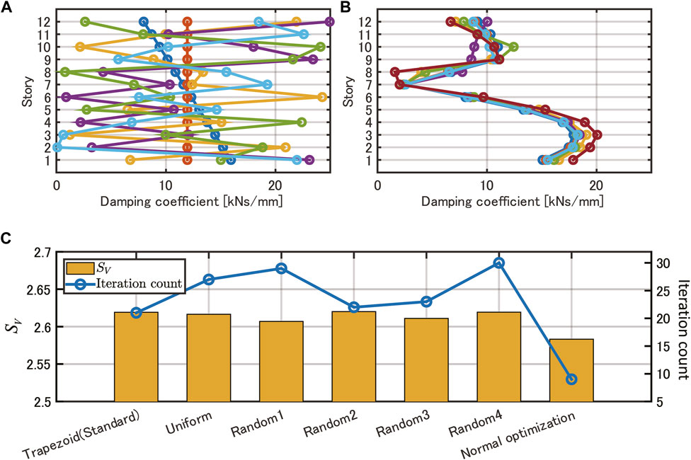
FIGURE 13. Investigation of initial solution dependence for robust optimization: (A) initial solution for random combinations, (B) optimal damping coefficient distribution, and (C) objective function in robust optimization and number of iterations.

6 Conclusion

A robustness evaluation method considering a wide range of input levels and performance criteria was presented for a structural design with various uncertainties. To address seismic input uncertainty in structural design, this paper focused on a worst-case scenario by utilizing a critical one-cycle sine wave, which establishes an upper bound on the structural response. In addition to the design constraint of the maximum response, the proposed robustness index evaluates the change in the robustness function with respect to variations in input amplitude as a multidimensional function. Furthermore, using the proposed robustness index, a robust optimal design problem and its solution method are presented to find a design that can retain high performance under uncertain parameters and large fluctuations in input levels. By solving numerical examples, the solution to the proposed robust optimization problem was presented using an elastoplastic shear mass system model with oil dampers. The detailed results obtained by this paper are as follows.

1) A simplified double impulse method is employed, where the main part of the near-fault seismic motions is expressed in terms of amplitude and impulse interval parameters. Based on the pre-analysis of the critical double impulse for the worst seismic input to the building structure, it is possible to take into account the uncertainty of the input. The effectiveness of the one-cycle sine wave, equivalent to the critical double impulse, in evaluating the structural response of inter-story ductility and floor accelerations was confirmed.

2) The uncertainty analysis method, obtaining the upper bound of the objective function under the specified uncertainty degrees, was applied to the robustness evaluation by varying the uncertainty range in a variable manner. The uncertainty analysis method was applicable for deriving the proposed robustness function considering both input velocity amplitude and performance criteria. The three-dimensional robustness surface was continuously derived by applying the interpolation of the cubic surface function.

3) The robust optimal damper placement problem, aiming to determine the damping coefficients of the oil dampers for each story, for the purpose of improving the volume value for the robustness surface was proposed. In order to consider the wide range of the input level and structural performance criteria, the volume integration value of the robustness surface was employed as the objective function of the optimal design problem.

4) The numerical examples were presented using an elastoplastic 12-degrees-of-freedom model for several optimization problems. The robust optimal design was compared with the normal optimal design where variations in oil dampers are not considered. It was shown that robust optimization can successively enhance the robustness by rearranging the damping coefficient under a constant constraint of the sum of damping coefficients. It was confirmed that in robust optimization, the damping coefficients are increased at specific floors with larger maximum ductility ratios when the degree of damper variation is increased. The investigation into the initial solution dependence revealed that a more robust solution can be achieved with a smaller computational load by using the normal optimal design as the initial solution.

Data availability statement

The original contributions presented in the study are included in the article/Supplementary Material; further inquiries can be directed to the corresponding author.

Author contributions

MH: conceptualization, data curation, formal analysis, investigation, and writing–original draft. KF: resources, supervision, validation, visualization, and writing–review and editing.

Funding

The author(s) declare financial support was received for the research, authorship, and/or publication of this article. This research was supported by JSPS, KAKENHI Grant No. 21K04334.

Conflict of interest

The authors declare that the research was conducted in the absence of any commercial or financial relationships that could be construed as a potential conflict of interest.

Publisher’s note

All claims expressed in this article are solely those of the authors and do not necessarily represent those of their affiliated organizations, or those of the publisher, the editors, and the reviewers. Any product that may be evaluated in this article, or claim that may be made by its manufacturer, is not guaranteed or endorsed by the publisher.

References

Akehashi, H., and Takewaki, I. (2019). Optimal viscous damper placement for elastic-plastic MDOF structures under critical double impulse. Front. Built Environ. 5, 20. doi:10.3389/fbuil.2019.00020

CrossRef Full Text | Google Scholar

Ben-Haim, Y. (2006). Info-gap decision theory: decisions under severe uncertainty. Amsterdam, Netherlands: Elsevier.

Google Scholar

Ben-Haim, Y., and Elishakoff, I. (1990). Convex models of uncertainty in applied mechanics. New York, NY, USA: Elsevier.

Google Scholar

Castaldo, P., and De Iuliis, M. (2014). Optimal integrated seismic design of structural and viscoelastic bracing-damper systems. Earthq. Eng. Struct. Dyn. 43 (12), 1809–1827. doi:10.1002/eqe.2425

CrossRef Full Text | Google Scholar

Chen, S. H., Ma, L., Meng, G. W., and Guo, R. (2009). An efficient method for evaluating the natural frequencies of structures with uncertain-but-bounded parameters. Comput. Struct. 87 (9-10), 582–590. doi:10.1016/j.compstruc.2009.02.009

CrossRef Full Text | Google Scholar

Doltsinis, I., and Kang, Z. (2004). Robust design of structures using optimization methods. Comput. Methods Appl. Mech. Eng. 193 (23-26), 2221–2237. doi:10.1016/j.cma.2003.12.055

CrossRef Full Text | Google Scholar

Elishakoff, I., and Ohsaki, M. (2010). Optimization and anti-optimization of structures under uncertainty. London: Imperial College Press.

Google Scholar

Faes, M., and Moens, D. (2020). Recent trends in the modeling and quantification of non-probabilistic uncertainty. Archives Comput. Methods Eng. 27, 633–671. doi:10.1007/s11831-019-09327-x

CrossRef Full Text | Google Scholar

Fragiadakis, M., and Papadrakakis, M. (2008). Performance-based optimum seismic design of reinforced concrete structures. Earthq. Eng. Struct. Dyn. 37 (6), 825–844. doi:10.1002/eqe.786

CrossRef Full Text | Google Scholar

Fujita, K., and Takewaki, I. (2011). An efficient methodology for robustness evaluation by advanced interval analysis using updated second-order Taylor series expansion. Eng. Struct. 33 (12), 3299–3310. doi:10.1016/j.engstruct.2011.08.029

CrossRef Full Text | Google Scholar

Fujita, K., Wataya, R., and Takewaki, I. (2021). Robust optimal damper placement of nonlinear oil dampers with uncertainty using critical double impulse. Front. Built Environ. 7, 744973. doi:10.3389/fbuil.2021.744973

CrossRef Full Text | Google Scholar

Fujita, K., and Yasuda, K. (2016). Robust optimization for damper placement under structural uncertainties using robustness function. J. Struct. Eng. AIJ 62B, 387–394. (in Japanese). doi:10.3130/aijjse.69B.0_181

CrossRef Full Text | Google Scholar

Garivani, S., Askariani, S. S., and Aghakouchak, A. A. (2020). “Seismic design of structures with yielding dampers based on drift demands,” in Structures (Amsterdam, Netherlands: Elsevier). doi:10.1016/j.istruc.2020.10.019

CrossRef Full Text | Google Scholar

Gholizadeh, S. (2015). Performance-based optimum seismic design of steel structures by a modified firefly algorithm and a new neural network. Adv. Eng. Softw. 81, 50–65. doi:10.1016/j.advengsoft.2014.11.003

CrossRef Full Text | Google Scholar

Gokkaya, B. U., Baker, J. W., and Deierlein, G. G. (2016). Quantifying the impacts of modeling uncertainties on the seismic drift demands and collapse risk of buildings with implications on seismic design checks. Earthq. Eng. Struct. Dyn. 45 (10), 1661–1683. doi:10.1002/eqe.2740

CrossRef Full Text | Google Scholar

Henriques, A. A., Veiga, J. M. C., Matos, J. A. C., and Delgado, J. M. (2008). Uncertainty analysis of structural systems by perturbation techniques. Struct. Multidiscip. Optim. 35 (3), 201–212. doi:10.1007/s00158-007-0218-z

CrossRef Full Text | Google Scholar

Hisada, Y., and Tanaka, S. (2021). What is fling step? Its theory, simulation method, and applications to strong ground motion near surface fault ruptures. Bull. Seismol. Soc. Am. 111 (5), 2486–2506. doi:10.1785/0120210046

CrossRef Full Text | Google Scholar

Hosoda, M., and Fujita, K. (2023). Robust Optimal Design based on Story ductility ratio of elastic-plastic building structures with uncertain oil dampers subjected to critical double impulse. J. Struct. Eng. B 69B, 181–189. (in Japanese). doi:10.3130/aijjse.69B.0_181

CrossRef Full Text | Google Scholar

Kaveh, A., Azar, B. F., Hadidi, A., Sorochi, F. R., and Talatahari, S. (2010). Performance-based seismic design of steel frames using ant colony optimization. J. Constr. Steel Res. 66 (4), 566–574. doi:10.1016/j.jcsr.2009.11.006

CrossRef Full Text | Google Scholar

Kojima, K., and Takewaki, I. (2015). Critical earthquake response of elastic–plastic structures under near-fault ground motions (Part 1: fling-step input). Front. Built Environ. 1, 12. doi:10.3389/fbuil.2015.00012

CrossRef Full Text | Google Scholar

Kojima, K., and Takewaki, I. (2016). Closed-form critical earthquake response of elastic-plastic structures with bilinear hysteresis under near-fault ground motions. J. Struct. Constr. Eng. 726, 1209–1219. (in Japanese). doi:10.3130/aijs.81.1209

CrossRef Full Text | Google Scholar

Lagaros, N. D., and Papadrakakis, M. (2007). Robust seismic design optimization of steel structures. Struct. Multidiscip. Optim. 33, 457–469. doi:10.1007/s00158-006-0047-5

CrossRef Full Text | Google Scholar

Moens, D., and Hanss, M. (2011). Non-probabilistic finite element analysis for parametric uncertainty treatment in applied mechanics: recent advances. Finite Elem. Analysis Des. 47 (1), 4–16. doi:10.1016/j.finel.2010.07.010

CrossRef Full Text | Google Scholar

Moens, D., and Vandepitte, D. (2004). An interval finite element approach for the calculation of envelope frequency response functions. Int. J. Numer. Methods Eng. 61 (14), 2480–2507. doi:10.1002/nme.1159

CrossRef Full Text | Google Scholar

Nabid, N., Hajirasouliha, I., Margarit, D. E., and Petkovski, M. (2020). Optimum energy based seismic design of friction dampers in RC structures. Structures 27, 2550–2562. doi:10.1016/j.istruc.2020.08.052

CrossRef Full Text | Google Scholar

Papavasileiou, G. S., and Charmpis, D. C. (2016). Seismic design optimization of multi–storey steel–concrete composite buildings. Comput. Struct. 170, 49–61. doi:10.1016/j.compstruc.2016.03.010

CrossRef Full Text | Google Scholar

Takewaki, I., and Ben-Haim, Y. (2005). Info-gap robust design with load and model uncertainties. J. Sound Vib. 288 (3), 551–570. doi:10.1016/j.jsv.2005.07.005

CrossRef Full Text | Google Scholar

Wang, C., Qiang, X., Fan, H., Wu, T., and Chen, Y. (2022). Novel data-driven method for non-probabilistic uncertainty analysis of engineering structures based on ellipsoid model. Comput. Methods Appl. Mech. Eng. 394, 114889. doi:10.1016/j.cma.2022.114889

CrossRef Full Text | Google Scholar

Xiao, Y., Zhou, Y., and Huang, Z. (2021). Efficient direct displacement-based seismic design approach for structures with viscoelastic dampers. Structures 29, 1699–1708. doi:10.1016/j.istruc.2020.12.067

CrossRef Full Text | Google Scholar

Zhang, R. H., and Soong, T. T. (1992). Seismic design of viscoelastic dampers for structural applications. J. Struct. Eng. 118 (5), 1375–1392. doi:10.1061/(asce)0733-9445(1992)118:5(1375)

CrossRef Full Text | Google Scholar