Critical pseudo-double impulse analysis evaluating seismic energy input to reinforced concrete buildings with steel damper columns

1 Introduction

1.1 Background and motivation

A dual system with sacrificial members that absorb the seismic energy prior to the beams and columns, e.g., a damage-tolerant structure (Wada et al., 2000), is one solution for creating structures with superior seismic performance. Unlike traditional earthquake-resistant structures, beams and columns in such dual systems are damage free (or have limited damage) after large earthquakes because most of the seismic energy input is absorbed by the sacrifice members. Therefore, buildings with such dual systems are more resilient than those without sacrificial members.

Steel damper columns (SDCs; Katayama et al., 2000) are energy-dissipating sacrificial members that are suitable for reinforced concrete (RC) buildings and are often used for multistory housing. The purpose of SDCs is to mitigate damage to beams and columns during strong seismic events. The author’s research group has been studying the seismic rehabilitation of existing RC buildings using SDCs (Fujii and Miyagawa, 2018; Fujii et al., 2019a) and the seismic design of new RC moment-resisting frames (MRFs) with SDCs (Mukoyama et al., 2021).

The peak deformation and cumulative strain energy are essential parameters in assessing the seismic performance of structural members. Specifically, the peak deformation is an essential parameter for RC members dominated by flexural behavior, as long as the story drift does not exceed 2.0% (Elwood et al., 2021). Meanwhile, both the peak deformation and the cumulative strain energy are important for the steel damper panels within SDCs. The residual displacement (Farrow and Kurama, 2003) is also important parameter, especially when the repair of the structures after earthquake is concerned. This is also important when the seismic sequence is considered (Ruiz-García and Negrete-Manriquez, 2011; Ruiz-García, 2012a, 2012b; Tesfamariam and Goda, 2015; Hoveidae and Radpour, 2021; Fujii, 2022). Specifically, Hoveidae and Radpour (2021) had pointed out that the large residual displacement after mainshock can significantly increase the peak response under aftershock.

In a previous paper, an energy-based prediction procedure for the peak and cumulative responses of an RC MRF building with SDCs was proposed (Fujii and Shioda, 2023). In this procedure, the building model is converted to an equivalent single-degree-of-freedom (SDOF) model that represents the first modal response. Then, two energy-related seismic intensity parameters are considered, namely, the maximum momentary input energy (Hori and Inoue, 2002) and the total input energy (Akiyama, 1985). The peak displacement is predicted by considering the energy balance during a half cycle of the structural response using the maximum momentary input energy. Meanwhile, the energy dissipation demand of the dampers is predicted considering the energy balance during an entire response cycle using the total input energy.

This procedure has been verified by comparing nonlinear time-history analysis (NTHA) results using non-pulse-like artificial ground motions (Fujii and Shioda, 2023) and 30 recorded pulse-like ground motions (Fujii, 2023b). However, the following issues remain.

I. In the presented procedure (Fujii and Shioda, 2023), the accuracy of the equivalent velocity of the maximum momentary input energy of the first modal response (${V_{\Delta E1}}^{*}$)–equivalent displacement of the first modal response (${D_1}^{*}$) relationship is essential for high quality predictions of the peak displacement. Accordingly, a monotonic pushover analysis was performed to evaluate the ${V_{\Delta E1}}^{*}$–${D_1}^{*}$ relationship. However, the strain hardening effect observed in low-yield steel shear panels subjected to cyclic loading (Nakashima, 1995) cannot be considered in a monotonic pushover analysis.

II. For the prediction of the peak equivalent displacement (${D_1}_{\max }^{*}$) and cumulative input energy of the first modal response, the equivalent velocities of the maximum momentary input energy (${V_{\Delta E1}}^{*}$) and the total input energy (${V_{I1}}^{*}$) are predicted from the linear elastic spectrum (the $V_{\Delta E}$ and $V_I$ spectra, respectively). In the presented procedure (Fujii and Shioda, 2023), the effective period of the first modal response (${T_1}_{eff}$) calculated from the predicted ${V_{\Delta E1}}^{*}$–${D_1}^{*}$ relationship is used for the predictions of ${V_{\Delta E1}}^{*}$ and ${V_{I1}}^{*}$. Although the accuracies of the predicted ${V_{\Delta E1}}^{*}$ and ${V_{I1}}^{*}$ values have been examined by comparing the predicted results with the NTHA results, the accuracy of ${T_1}_{eff}$ has not yet been examined. The response period of the first modal response (${T_1}_{res}$), which is defined as twice $\Delta t$ ( where $\Delta t$ is the interval of a half cycle of the structural response), is a good index for evaluating ${T_1}_{eff}$ in NTHA results. However, the value of $\Delta t$ obtained from the NTHA results is unstable because of the complexity of the characteristics of ground motions and the influence of the higher modal responses of a structure.

The relationship between the energy and the peak deformation has been studied by several researchers. There are two main approaches: the first approach is to define a parameter that relates the cumulative input energy (or cumulative strain energy) and the peak deformation, and the second approach is to define an energy-based seismic intensity parameter that is directly related to the peak deformation. Akiyama (1988) stated that the cumulative inelastic deformation ratio should be assumed to be 4 times the peak inelastic deformation ratio for the seismic design of structures with elastic–perfectly plastic behavior, such as ductile steel MRFs. Then, the equivalent number of cycles can be formulated as the ratio of the cumulative inelastic deformation to the peak inelastic deformation in the simplified energy-based seismic design method (Akiyama, 1999). Manfredi and Cosenza (2003) investigated the relationship between the equivalent number of plastic cycles and the seismological parameters in the near field based on 128 near-fault and 122 far-fault records. They concluded that “the relative importance of the cyclic damage for structures grows at the higher distance from the fault, whereas in the near-source conditions structural response is governed by the peak demand, confirming the damage observations after destructive earthquakes.” Mota-Páez et al. (2021) noted that, for the seismic retrofit design of an RC soft-story building with a hysteresis damper under near-fault earthquakes, the equivalent number of cycles should be reduced. This is because, in the case of a near-fault earthquake, a large amount of seismic energy input occurs within a few cycles. Within the first approach, Fajfar (1992) proposed another dimensionless parameter $\gamma$ normalizing the cumulative hysteretic dissipated (strain) energy by the peak deformation. This parameter $\gamma$ has been applied to the pushover-based damage analysis method of RC MRFs (Gaspersic et al., 1992; Fajfar and Gaspersic, 1996) and the seismic design procedure of new RC MRFs (Teran-Gilmore, 1998). Decanini et al. (2000) studied the relationship between the cumulative input energy and the peak displacement of RC MRFs subjected to near-source earthquakes; they concluded that a reliable relationship between the cumulative energy and the peak displacement can be constructed, using either the cumulative hysteretic dissipated energy or the cumulative input energy. Mollaioli et al. (2011) analyzed the correlations between the energy and the peak displacement for linear and nonlinear SDOF and multi-degree-of-freedom (MDOF) models. Following these studies, Angelucci et al. (2023b) studied the relationship between the cumulative input energy and the peak displacement of RC MRFs with infills. Meanwhile, Benavent-Climent (Benavent-Climent et al., 2004; Benavent-Climent, 2011) proposed an energy-based assessment method for existing buildings; they focused on the strain energy under the monotonic loading of stories until the ultimate state, instead of the ultimate story drift.

Inoue and his research group (Hori et al., 2000; Inoue et al., 2000; Hori and Inoue, 2002) proposed the maximum momentary input energy as an energy-based seismic intensity parameter that is directly related to the peak displacement of RC structures. Note that a similar energy-based seismic intensity parameter was proposed by Kalkan and Kunnath (2007). The present authors formulated the time-varying function of the momentary energy input of an elastic SDOF model using Fourier series (Fujii et al., 2019b). Then, the concept of the momentary input energy was extended to bidirectional horizontal excitation (Fujii, 2021; Fujii and Murakami, 2021). In addition, Fajfar’s $\gamma$ parameter was re-formulated using the maximum momentary input energy and the total input energy for RC structures (Fujii, 2021). Similarly, for base-isolated structures with hysteresis dampers, Akiyama’s equivalent number of cycles was reformulated using the maximum momentary input energy and the total input energy (Fujii, 2023a). Angelucci et al. (2023a) studied the relationship between the energy-related seismic intensity parameters proposed by Kalkan and Kunnath (2007) and the peak displacement of bare RC MRFs. The author thinks, there are two advantages in the concept of the maximum momentary input energy in comparison with the concept of equivalent number of cycles. The first is, the maximum momentary input energy can be evaluated from the complex Fourier coefficients of the input ground motion by using the time-varying function of the momentary energy input of an elastic SDOF model, as well as the cumulative input energy over the course of seismic input (Fujii et al., 2019a). The second is, theoretically, the concept of the maximum momentary input energy is easy to apply the structures with any type of hysteresis behavior, if the energy dissipation during a half cycle of structural response can be properly modeled: in the previous study by the author’s group (Fujii et al., 2021), the peak displacement of the RC structures with brittle members was predicted using the concept of the maximum momentary energy input. On the contrary, the equivalent number of cycles, investigated by Akiyama (1988), Akiyama (1999), Manfredi and Cosenza (2003), depends on so many parameters, e.g., the hysteresis models, ratio of the stiffness after yielding with respect to the initial stiffness, and type of ground motion (near-field or far-field). Therefore, the proposed equations of the equivalent number of cycles are empirical, which strongly relies on the numerical analysis results by using a certain ground motion set. In addition, from the author’s point of view, the prediction of the peak response based on the concept of maximum momentary energy input is straightforward, while its prediction based on the total energy input and the equivalent number of cycles is roundabout. Therefore, the author thinks that use of the two energy-based seismic intensity parameters, the maximum momentary input energy and the total input energy, is the best for evaluating the peak and cumulative response of building structures.

The above-discussed studies are based on NTHA results using recorded ground motions. Conversely, Takewaki and his research group (Kojima and Takewaki, 2015a; Kojima and Takewaki, 2015b; Kojima and Takewaki, 2015c; Kojima et al., 2015; Akehashi and Takewaki, 2021; Akehashi and Takewaki, 2022) studied simplifying the seismic input as a series of impulsive forces. First, Kojima et al. (2015) introduced the concept of the “critical double impulse input,” which represents the upper bound of the earthquake energy input for a given pulse velocity ($V_p$). Next, Kojima and Takewaki introduced the double impulse input as a substitute for the fling-step near-fault ground motion Kojima and Takewaki (2015a). Following this study, they introduced the triple impulse input as a substitute for the forward-directivity near-fault ground motion Kojima and Takewaki (2015b) and the multiple impulse input as a substitute for long-duration earthquake ground motion Kojima and Takewaki (2015c). Then, Akehashi and Takewaki introduced pseudo-double impulse (PDI) Akehashi and Takewaki (2021) and pseudo-multi impulse (PMI) Akehashi and Takewaki (2022) analyses. In PDI and PMI analyses, the MDOF model oscillates predominantly in a single mode, considering the impulsive lateral force corresponding to a certain mode vector; when the impulsive lateral force corresponding to the first mode vector is considered, the MDOF model oscillates predominantly in the first mode.

The author believes that PDI is suitable to discuss the above two issues (I and II) for the following reasons: 1) the momentary input energy can easily be calculated as the increment of the energy input as a result of the pseudo impulsive lateral force. And 2) the interval of a half cycle of the structural response ($\Delta t$) can easily be evaluated and is expected to be stable because the MDOF model oscillates predominantly in a single mode.

1.2 Objectives

Given the above-outlined background, this study addresses the following questions.

(i) What is the ${V_{\Delta E1}}^{*}$–${D_1}_{\max }^{*}$ relationship when considering the response of an RC MRF with SDCs subjected to critical PDI input? Does it agree with the predicted ${V_{\Delta E1}}^{*}$–${D_1}^{*}$ relationship from the simplified equation proposed in the author’s previous study (Fujii and Shioda, 2023)?

(ii) What is the relationship between the response period (${T_1}_{res}$) and the effective period (${T_1}_{eff}$) calculated from ${D_1}_{\max }^{*}$ and ${V_{\Delta E1}}^{*}$ in the case of an RC MRF with SDCs subjected to critical PDI input?

In this study, critical PDI analyses of RC MRF models are performed. These critical PDI analyses are based on studies by Akehashi and Takewaki (2021) with one modification: in this study, the change in the first mode shape in the nonlinear range is considered to maintain consistency with the assumptions applied in the procedure (Fujii and Shioda, 2023). Six 8- and 16-story RC MRFs with and without SDCs are analyzed considering various intensities of the pulse velocity $V_p$. Then, the predicted ${V_{\Delta E1}}^{*}$–${D_1}^{*}$ and ${T_1}_{eff}$–${D_1}^{*}$ relationships calculated according to the procedure (Fujii and Shioda, 2023) are compared with those obtained from the critical PDI analysis results.

Several researchers (McCormick et al., 2007; Tremblay et al., 2008) have investigated the response of structures with self-centering energy-dissipative devices to minimize the residual displacement after earthquake. In their studies, the behavior of devices is characterized by the flag-shaped hysteresis responses. The behavior of structures with such devices is out of scope of this study because the behavior of RC MRFs with SDCs is the main target of the following discussions. However, the author thinks the proposed procedure in the author’s previous study (Fujii and Shioda, 2023) can be easily extended to the structures with such self-centering energy-dissipative devices: only the modeling of the hysteretic dissipated energy during a half cycle of structural response is needed.

The rest of this paper is organized as follows. Section 2 outlines the critical PDI analysis based on Akehashi and Takewaki (2021). Section 3 presents the six RC MRFs with and without SDCs and the analysis methods. Section 4 describes the responses of the six RC MRFs obtained from the critical PDI analysis results. Section 5 discusses the comparisons with the predicted results based on the author’s previous study (Fujii and Shioda, 2023) and the critical PDI analysis results, focusing particularly on (i) the ${V_{\Delta E1}}^{*}$–${D_1}^{*}$ relationship and (ii) the $T_{1eff}$–${D_1}^{*}$ relationship. The conclusions drawn from this study and the directions of future research are discussed in Section 6.

2 Critical PDI analysis

2.1 Outline of the critical PDI analysis

Figure 1 outlines the critical PDI analysis. This analysis is based on the studies by Akehashi and Takewaki (2021), Akehashi and Takewaki (2022), and one modification is made to maintain consistency with the assumptions applied in the procedure (Fujii and Shioda, 2023): in this study, the change in the first mode vector (${\mathrm{\Gamma }}_1{\mathbf{\phi }}_{\mathbf{1}}$) in the nonlinear range is considered for the calculation of the first modal response at time $t$ and the second pseudo impulsive lateral force.

FIGURE 1

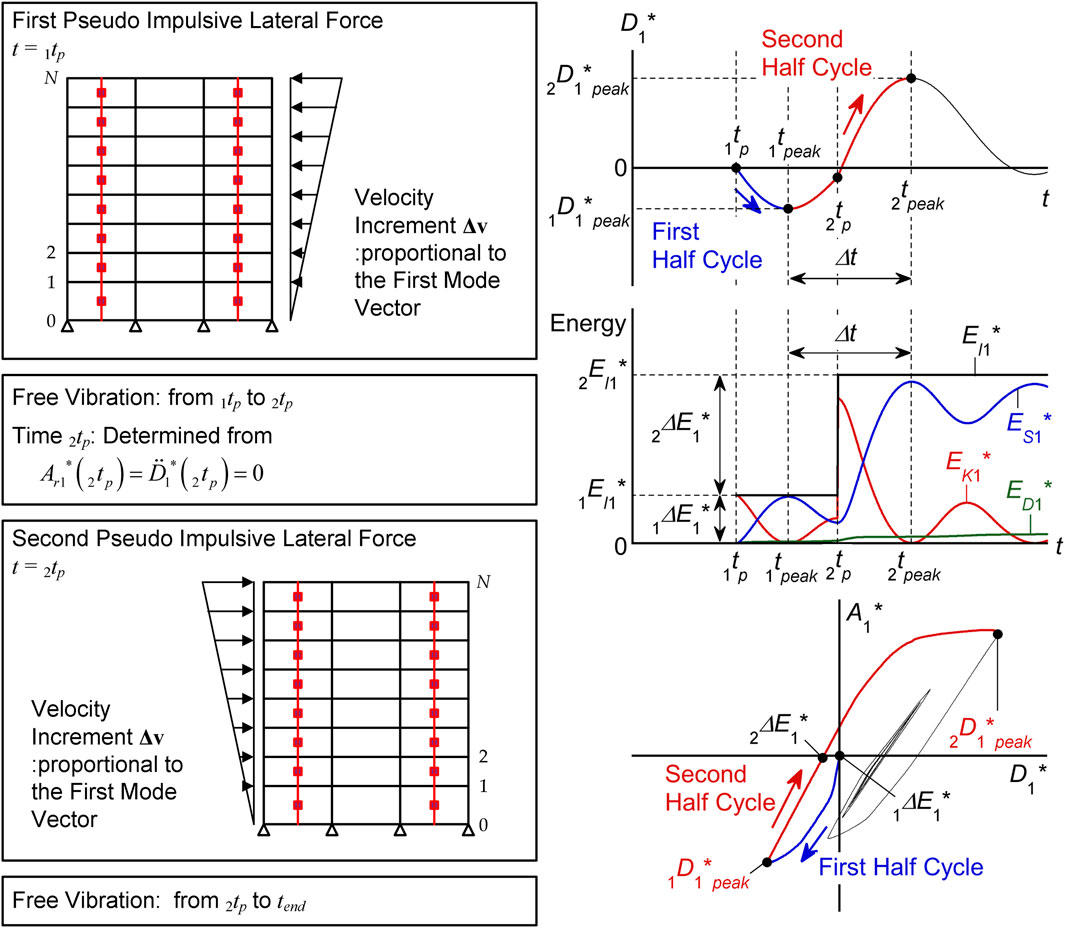
FIGURE 1. Outline of the critical pseudo-double impulse (PDI) analysis.

Consider a planer frame building model (number of stories, $N$) subjected to a pseudo impulsive lateral force proportional to the first mode vector (pulse velocity: $V_p$). Here, $\mathbf{M}$ is the mass matrix of the building model; $\mathbf{d}\left(t\right)$, $\mathbf{v}\left(t\right)$, and $\mathbf{a}\left(t\right)$ are the relative displacement, velocity, and acceleration vectors, respectively; and ${\mathbf{f}}_{\mathbf{R}}\left(t\right)$ and ${\mathbf{f}}_{\mathbf{D}}\left(t\right)$ are the restoring force and damping force vectors, respectively. The equivalent displacement ($D_1^{*}\left(t\right)$), equivalent velocity ($V_1^{*}\left(t\right)$), and equivalent relative acceleration ($A_{r1}^{*}\left(t\right)$) of the first modal response are defined as Eqs 1–3, respectively:

$D_1^{*}\left(t\right)=\frac{{\mathrm{\Gamma }}_1{{\mathbf{\phi }}_{\mathbf{1}}}^{\mathbf{T}}\mathbf{\text{Md}}\left(\mathit{\text{t}}\right)}{M_1^{*}},(1)$

$V_1^{*}\left(t\right)={{\dot{D}}_1}^{*}\left(t\right)=\frac{{\mathrm{\Gamma }}_1{{\mathbf{\phi }}_{\mathbf{1}}}^{\mathbf{T}}\mathbf{\text{Mv}}\left(t\right)}{M_1^{*}},(2)$

$A_{r1}^{*}\left(t\right)={{\ddot{D}}_1}^{*}\left(t\right)=\frac{{\mathrm{\Gamma }}_1{{\mathbf{\phi }}_{\mathbf{1}}}^{\mathbf{T}}\mathbf{\text{Ma}}\left(t\right)}{M_1^{*}},(3)$

$M_1^{*}={{\mathrm{\Gamma }}_1}^2{{\mathbf{\phi }}_{\mathbf{1}}}^{\mathbf{T}}\mathbf{M}{\mathbf{\phi }}_{\mathbf{1}},(4)$

where ${M_1}^{*}$ defined as Eq. 4 is the effective first modal mass. Note that ${\mathrm{\Gamma }}_1{\mathbf{\phi }}_{\mathbf{1}}$ and ${M_1}^{*}$ depend on the local maximum equivalent displacement within the range $\left(0,t\right)$. In this study, the first mode vector at time $t$ is updated assuming that ${\mathrm{\Gamma }}_1{\mathbf{\phi }}_{\mathbf{1}}$ is proportional to the displacement vector at the time when the maximum equivalent displacement occurs ($t_{\max }$). The first mode vector at time $t$ is updated according to Eq. 5:

${\mathrm{\Gamma }}_1{\mathbf{\phi }}_{\mathbf{1}}\leftarrow \frac{1}{{D_1}^{*}\left(t_{\max }\right)}\mathbf{d}\left(t_{\max }\right).(5)$

The equivalent acceleration ${A_1}^{*}\left(t\right)$ is defined as Eq. 6:

${A_1}^{*}\left(t\right)=\frac{{\mathrm{\Gamma }}_1{{\mathbf{\phi }}_{\mathbf{1}}}^{\mathbf{T}}{\mathbf{f}}_{\mathbf{R}}\left(t\right)}{{M_1}^{*}}.(6)$

2.1.1 First pseudo impulsive lateral force

At time $t={}_1{t}_p\left({}_1{t}_p>0\right)$, the first pseudo impulsive lateral force acts on the building model, as shown in Figure 1. Note that, before the first pseudo impulsive force acts on the building model ($t<{}_1{t}_p$), the building model is in the stationary state ($\mathbf{d}\left(t\right)=\mathbf{0}$, $\mathbf{v}\left(t\right)=\mathbf{0}$, $\mathbf{a}\left(t\right)=\mathbf{0}$). The equivalent velocity of the first modal response just after the first pseudo impulsive lateral force acts (${{\stackrel{\sim }{V}}_1}^{*}\left({}_1{t}_p\right)$) is calculated as Eq. 7:

${{\stackrel{\sim }{V}}_1}^{*}\left({}_1{t}_p\right)=-V_p.(7)$

Then the corresponding velocity vector ($\stackrel{\sim }{\mathbf{v}}\left({}_1{t}_p\right)$) is calculated as Eq. 8:

$\stackrel{\sim }{\mathbf{v}}\left({}_1{t}_p\right)={}_1{\mathrm{\Gamma }}_1{}_1{\mathbf{\phi }}_{\mathbf{1}}{{\stackrel{\sim }{V}}_1}^{*}\left({}_1{t}_p\right)=-{}_1{\mathrm{\Gamma }}_1{}_1{\mathbf{\phi }}_{\mathbf{1}}{V}_p,(8)$

where ${}_1{\mathrm{\Gamma }}_1{}_{\mathbf{1}}{\mathbf{\phi }}_{\mathbf{1}}$ is the first mode vector at the initial stage. The increment of the input energy of the first modal response (${}_1\Delta {E_1}^{*}$) is calculated as Eq. 9:

${}_1\Delta {E_1}^{*}=\frac{1}{2}{}_1{M_1}^{*}{\left\{{{\stackrel{\sim }{V}}_1}^{*}\left({}_1{t}_p\right)\right\}}^2=\frac{1}{2}{}_1{M_1}^{*}{V_p}^2,(9)$

where ${}_1{M_1}^{*}$ is the first modal mass at the initial stage. The cumulative input energy of the first modal response (${}_1{E_{I1}}^{*}$) is calculated as Eq. 10:

${}_1{E_{I1}}^{*}={}_1\Delta {E_1}^{*}.(10)$

To calculate the response following the action of the first pseudo impulsive lateral force, the equivalent velocity (${V_1}^{*}\left(t\right)$) and the velocity vector ($\mathbf{v}\left(t\right)$) are updated according to Eq. 11:

${V_1}^{*}\left({}_1{t}_p+0\right)\leftarrow {{\stackrel{\sim }{V}}_1}^{*}\left({}_1{t}_p\right),\mathbf{v}\left({}_1{t}_p+0\right)\leftarrow \stackrel{\sim }{\mathbf{v}}\left({}_1{t}_p\right).(11)$

2.1.2 Free vibration after the first pseudo impulsive lateral force

Following the action of the first pseudo impulsive lateral force, the building model oscillates without external forces (free vibration) until the arrival of the second pseudo impulsive lateral force. The kinetic energy, damping dissipated energy, cumulative strain energy, and cumulative input energy of the first modal response (${E_{K1}}^{*}$, ${E_{D1}}^{*}$, ${E_{S1}}^{*}$, and ${E_{I1}}^{*}$, respectively) are expressed as Eqs 12–15, respectively:

${E_{K1}}^{*}\left(t\right)=\frac{1}{2}{M_1}^{*}{\left\{{V_1}^{*}\left(t\right)\right\}}^2,(12)$

${E_{D1}}^{*}\left(t\right)={\displaystyle \underset{0}{\overset{t}{\int }}}{\mathrm{\Gamma }}_1{{\mathbf{\phi }}_{\mathbf{1}}}^{\mathbf{T}}{\mathbf{f}}_{\mathbf{D}}\left(t\right){V_1}^{*}\left(t\right)dt,(13)$

${E_{S1}}^{*}\left(t\right)={\displaystyle \underset{0}{\overset{t}{\int }}}{\mathrm{\Gamma }}_1{{\mathbf{\phi }}_{\mathbf{1}}}^{\mathbf{T}}{\mathbf{f}}_{\mathbf{R}}\left(t\right){V_1}^{*}\left(t\right)dt,(14)$

${E_{I1}}^{*}\left(t\right)=\frac{1}{2}{}_1{M_1}^{*}{V_p}^2={}_1{E_{I1}}^{*}.(15)$

Because the first pseudo impulsive lateral force is proportional to the first mode vector, the building model oscillates predominantly in the first mode. Therefore, the kinetic energy, damping dissipated energy, cumulative strain energy, and cumulative input energy ($E_K$, $E_D$, $E_S$, and $E_I$, respectively) are approximated as Eq. 16:

$\left\{\begin{array}{l}{E}_K\left(t\right)\approx {E_{K1}}^{*}\left(t\right)\\ E_D\left(t\right)\approx {E_{D1}}^{*}\left(t\right)\\ E_S\left(t\right)\approx {E_{S1}}^{*}\left(t\right)\\ E_I\left(t\right)\approx {E_{I1}}^{*}\left(t\right)\end{array}\right..(16)$

Note that the first mode vector (${\mathrm{\Gamma }}_1{\mathbf{\phi }}_{\mathbf{1}}$) updates any step according to Eq. 5 until ${D_1}^{*}\left(t\right)$ reaches its local peak (${}_1{D_1}_{peak}^{*}\left(<0\right)$ shown in Figure 1) and that the effective first modal mass (${M_1}^{*}$) is re-calculated according to Eq. 4. The time ${}_1{t}_{peak}$ is defined as the time when ${D_1}^{*}\left(t\right)$ reaches ${}_1{D_1}_{peak}^{*}$.

The timing of the second pseudo impulsive lateral force (${}_2{t}_p>{}_1{t}_p$) is determined from the following condition:

${{\dot{V}}_1}^{*}\left({}_2{t}_p\right)={A_{r1}}^{*}\left({}_2{t}_p\right)=0.(17)$

This condition (Eq. 17) is equivalent to the condition of critical timing given by Akehashi and Takewaki (2021), Akehashi and Takewaki (2022).

2.1.3 Second pseudo impulsive lateral force

At time $t={}_2{t}_p$, the second pseudo impulsive lateral force acts on the building model, as shown in Figure 1. The equivalent velocity of the first modal response just after the arrival of the second pseudo impulsive lateral force (${{\stackrel{\sim }{V}}_1}^{*}\left({}_2{t}_p\right)$) is calculated as Eq. 18:

${{\stackrel{\sim }{V}}_1}^{*}\left({}_2{t}_p\right)={V_1}^{*}\left({}_2{t}_p-0\right)+V_p.(18)$

Here, ${V_1}^{*}\left({}_2{t}_p-0\right)$ is the equivalent velocity of the first modal response just before the action of the second pseudo impulsive lateral force. Assuming that the velocity vector just prior to the action of the second pseudo impulsive lateral force ($\mathbf{v}\left({}_2{t}_p-0\right)$) can be approximated by the first modal response, the corresponding velocity vector ($\stackrel{\sim }{\mathbf{v}}\left({}_2{t}_p\right)$) can be expressed as Eq. 19:

$\stackrel{\sim }{\mathbf{v}}\left({}_2{t}_p\right)=\mathbf{v}\left({}_2{t}_p-0\right)+{\mathrm{\Gamma }}_1{\mathbf{\phi }}_{\mathbf{1}}{V}_p\approx {\mathrm{\Gamma }}_1{\mathbf{\phi }}_{\mathbf{1}}{{\stackrel{\sim }{V}}_1}^{*}\left({}_2{t}_p\right).(19)$

The increment of the input energy of the first modal response (${}_2\Delta {E_1}^{*}$) is calculated as Eq. 20:

${}_2\Delta {E_1}^{*}=\frac{1}{2}{M_1}^{*}\left[{\left\{{{\stackrel{\sim }{V}}_1}^{*}\left({}_2{t}_p\right)\right\}}^2-{\left\{{V_1}^{*}\left({}_2{t}_p-0\right)\right\}}^2\right]=\frac{1}{2}{M_1}^{*}{V_p}^2\left\{1+\frac{2{V_1}^{*}\left({}_2{t}_p-0\right)}{V_p}\right\}.(20)$

Note that Eq. 17 is obtained by differentiating Eq. 20 with respect to ${}_2{t}_p$ and equating it to zero. Therefore, the timing of the arrival of the second pseudo impulsive lateral force is the timing that maximizes ${}_2\Delta {E_1}^{*}$.

The cumulative input energy of the first modal response immediately following the action of the second pseudo impulsive lateral force (${}_2{E_{I1}}^{*}$) is calculated as Eq. 21:

${}_2{E_{I1}}^{*}={}_1\Delta {E_1}^{*}+{}_2\Delta {E_1}^{*}.(21)$

To calculate the response following the action of the second pseudo impulsive lateral force, the equivalent velocity (${V_1}^{*}\left(t\right)$) and the velocity vector ($\mathbf{v}\left(t\right)$) are updated according to Eq. 22:

${V_1}^{*}\left({}_2{t}_p+0\right)\leftarrow {{\stackrel{\sim }{V}}_1}^{*}\left({}_2{t}_p\right),\mathbf{v}\left({}_2{t}_p+0\right)\leftarrow \stackrel{\sim }{\mathbf{v}}\left({}_2{t}_p\right).(22)$

2.1.4 Free vibration after the second pseudo impulsive lateral force

Following the action of the second pseudo impulsive lateral force, the building model oscillates without external forces (free vibration) until $t=t_{end}$.

The time ${}_2{t}_{peak}$ is defined as the time when ${D_1}^{*}\left(t\right)$ reaches its local peak (${}_2{D_1}_{peak}^{*}\left(>0\right)$). The peak equivalent displacement of the first modal response over the course of the entire seismic event (${D_1}_{\max }^{*}$) is defined as Eq. 23:

${D_1}_{\max }^{*}=\max \left(\left|{}_1{D_1}_{peak}^{*}\right|,\left|{}_2{D_1}_{peak}^{*}\right|\right).(23)$

2.2 Momentary input energy in the critical PDI analysis

Consider the energy response of the equivalent SDOF model representing the first modal response subjected to the ground acceleration ($a_g\left(t\right)$). The cumulative input energy of the first modal response per unit mass over the course of the entire seismic event (${E_{I1}}^{*}/{M_1}^{*}$) is calculated from the time derivative of the equivalent displacement (${{\dot{D}}_1}^{*}\left(t\right)={V_1}^{*}\left(t\right)$) and the ground acceleration ($a_g\left(t\right)$) as Eq. 24:

$\frac{{E_{I1}}^{*}}{{M_1}^{*}}=-{\displaystyle \underset{0}{\overset{t_{end}}{\int }}}{a}_g\left(t\right)\cdot {{\dot{D}}_1}^{*}\left(t\right)dt=-{\displaystyle \underset{0}{\overset{t_{end}}{\int }}}{a}_g\left(t\right)\cdot {V_1}^{*}\left(t\right)dt.(24)$

According to Hori and Inoue (2002), the momentary input energy of the first modal response per unit mass ($\Delta {E_1}^{*}/{M_1}^{*}$) is calculated as Eq. 25:

$\frac{\Delta {E_1}^{*}}{{M_1}^{*}}=-{\displaystyle \underset{t}{\overset{t+\Delta t}{\int }}}{a}_g\left(t\right)\cdot {V_1}^{*}\left(t\right)dt.(25)$

In Eq. 25, $t$ and $t+\Delta t$ are the beginning and ending times of a half cycle of the structural response, respectively. The maximum momentary input energy per unit mass ($\Delta {E_1}_{\max }^{*}/{M_1}^{*}$) is defined as the maximum value of $\Delta {E_1}^{*}/{M_1}^{*}$ over the course of the entire seismic event.

Following the study by Kojima and Takewaki (2015a), the ground acceleration ($a_g\left(t\right)$) in the case of a critical DI analysis can be written as Eq. 26:

$a_g\left(t\right)=V_p\left\{\delta \left(t-{}_1{t}_p\right)-\delta \left(t-{}_2{t}_p\right)\right\}.(26)$

In Eq. 26, $\delta \left(·\right)$ is the Dirac delta function, which satisfies Eq. 27:

$\left.\begin{array}{l}\delta \left(t\right)=\underset{\epsilon \to +0}{\lim }\left\{\begin{array}{cc}0& \left|t\right|>\epsilon \\ \frac{1}{2\epsilon }& \left|t\right|\le \epsilon \end{array}\right.\\ {\displaystyle \underset{-\infty }{\overset{\infty }{\int }}}\delta \left(t\right)dt=1\\ {\displaystyle \underset{-\infty }{\overset{\infty }{\int }}}\delta \left(t\right)f\left(t\right)dt=f\left(0\right)\end{array}\right\}.(27)$

Next, the momentary input energy of the first modal response per unit mass at the first and second half cycles (${}_1\left(\Delta {E_1}^{*}/{M_1}^{*}\right)$ and ${}_2\left(\Delta {E_1}^{*}/{M_1}^{*}\right)$, respectively) are calculated from Eqs 25, 26. Assuming that the intervals of the first and second half cycles of the structural response are $\left[0,{}_1{t}_{peak}\right]$ and $\left[{}_1{t}_{peak},{}_2{t}_{peak}\right]$, respectively, as shown in Figure 1, ${}_1\left(\Delta {E_1}^{*}/{M_1}^{*}\right)$ and ${}_2\left(\Delta {E_1}^{*}/{M_1}^{*}\right)$ can be calculated as Eqs 28, 29:

${}_1\left(\frac{\Delta {E_1}^{*}}{{M_1}^{*}}\right)=-{\displaystyle \underset{0}{\overset{{}_1{t}_{peak}}{\int }}}{a}_g\left(t\right)\cdot {V_1}^{*}\left(t\right)dt,(28)$

${}_2\left(\frac{\Delta {E_1}^{*}}{{M_1}^{*}}\right)=-{\displaystyle \underset{{}_1{t}_{peak}}{\overset{{}_2{t}_{peak}}{\int }}}{a}_g\left(t\right)\cdot {V_1}^{*}\left(t\right)dt.(29)$

Note that, in Eq. 28, the interval of integration is changed from $\left[{}_1{t}_p,{}_1{t}_{peak}\right]$ to $\left[0,{}_1{t}_{peak}\right]$ to calculate the integrals that contain the Dirac delta function. To calculate Eqs 28, 29, the equivalent velocities (${V_1}^{*}\left(t\right)$) at times $t={}_1{t}_p$ and $t={}_2{t}_p$ are rewritten as Eqs 30, 31, respectively:

${V_1}^{*}\left({}_1{t}_p\right)=\frac{1}{2}\left\{{V_1}^{*}\left({}_1{t}_p-0\right)+{V_1}^{*}\left({}_1{t}_p+0\right)\right\}=-\frac{1}{2}{V}_p,(30)$

${V_1}^{*}\left({}_2{t}_p\right)=\frac{1}{2}\left\{{V_1}^{*}\left({}_2{t}_p-0\right)+{V_1}^{*}\left({}_2{t}_p+0\right)\right\}={V_1}^{*}\left({}_2{t}_p-0\right)+\frac{1}{2}{V}_p.(31)$

Therefore, ${}_1\left(\Delta {E_1}^{*}/{M_1}^{*}\right)$ and ${}_2\left(\Delta {E_1}^{*}/{M_1}^{*}\right)$ can be calculated as Eqs 32, 33, respectively:

${}_1\left(\frac{\Delta {E_1}^{*}}{{M_1}^{*}}\right)=-V_p\cdot {V_1}^{*}\left({}_1{t}_p\right)=\frac{1}{2}{V_p}^2,(32)$

${}_2\left(\frac{\Delta {E_1}^{*}}{{M_1}^{*}}\right)=-\left(-V_p\right)\cdot {V_1}^{*}\left({}_2{t}_p\right)=\frac{1}{2}{V_p}^2\left\{1+\frac{2{V_1}^{*}\left({}_2{t}_p-0\right)}{V_p}\right\}.(33)$

The calculated ${}_1\left(\Delta {E_1}^{*}/{M_1}^{*}\right)$ and ${}_2\left(\Delta {E_1}^{*}/{M_1}^{*}\right)$ shown in Eqs 32, 33 are consistent with the above-shown increments of the energy input (Eqs 9, 20, respectively). This implies that, in the case of a critical PDI analysis, the momentary input energy is calculated as the increment of the energy input as a result of the pseudo impulsive lateral force.

The maximum momentary input energy of the first modal response per unit mass ($\Delta {E_1}_{\max }^{*}/{M_1}^{*}$) is obtained as Eq. 34:

$\frac{\Delta {E_1}_{\max }^{*}}{{M_1}^{*}}=\max \left\{{}_1\left(\frac{\Delta {E_1}^{*}}{{M_1}^{*}}\right),{}_2\left(\frac{\Delta {E_1}^{*}}{{M_1}^{*}}\right)\right\}={}_2\left(\frac{\Delta {E_1}^{*}}{{M_1}^{*}}\right)=\frac{1}{2}{V_p}^2\left\{1+\frac{2{V_1}^{*}\left({}_2{t}_p-0\right)}{V_p}\right\}.(34)$

The cumulative input energy of the first modal response per unit mass (${E_{I1}}^{*}/{M_1}^{*}$) is calculated as Eq. 35:

$\frac{{E_{I1}}^{*}}{{M_1}^{*}}={}_1\left(\frac{\Delta {E_1}^{*}}{{M_1}^{*}}\right)+{}_2\left(\frac{\Delta {E_1}^{*}}{{M_1}^{*}}\right)={V_p}^2\left\{1+\frac{{V_1}^{*}\left({}_2{t}_p-0\right)}{V_p}\right\}.(35)$

The equivalent velocity of the maximum momentary input energy of the first modal response (${V_{\Delta E1}}^{*}$) is calculated as Eq. 36:

${V_{\Delta E1}}^{*}=\sqrt{\frac{2\Delta {E_1}_{\max }^{*}}{{M_1}^{*}}}=V_p\sqrt{1+\frac{2{V_1}^{*}\left({}_2{t}_p-0\right)}{V_p}}.(36)$

Similarly, the equivalent velocity of the cumulative input energy of the first modal response (${V_{I1}}^{*}$) is calculated as Eq. 37:

${V_{I1}}^{*}=\sqrt{\frac{2{E_{I1}}^{*}}{{M_1}^{*}}}=\sqrt{2}\cdot V_p\sqrt{1+\frac{{V_1}^{*}\left({}_2{t}_p-0\right)}{V_p}.}(37)$

In this study, the response period of the first modal response ($T_{1res}$) is defined as twice the interval between the two local peaks (${}_1{D_1}_{peak}^{*}$ and ${}_2{D_1}_{peak}^{*}$) as Eq. 38:

$T_{1res}=2\Delta t=2\left({}_2{t}_{peak}-{}_1{t}_{peak}\right).(38)$

2.3 Analysis flow

Figure 2 shows the flow of the critical PDI analysis. In this flow, the damping force increment resulting from the velocity vector changing at analysis step $n$ (${}_{\mathbf{n}}\mathbf{v}$) is treated as the unbalanced force to be corrected in the next step. In addition, the timing of the second pseudo impulsive lateral force is determined by checking the sign of the equivalent relative acceleration (${}_n{A_{r1}}^{*}$). The timing of the second pseudo impulsive lateral force is determined according the following condition:

${}_n{A_{r1}}^{*}{}_{n+1}{A_{r1}}^{*}\le 0.(39)$

FIGURE 2

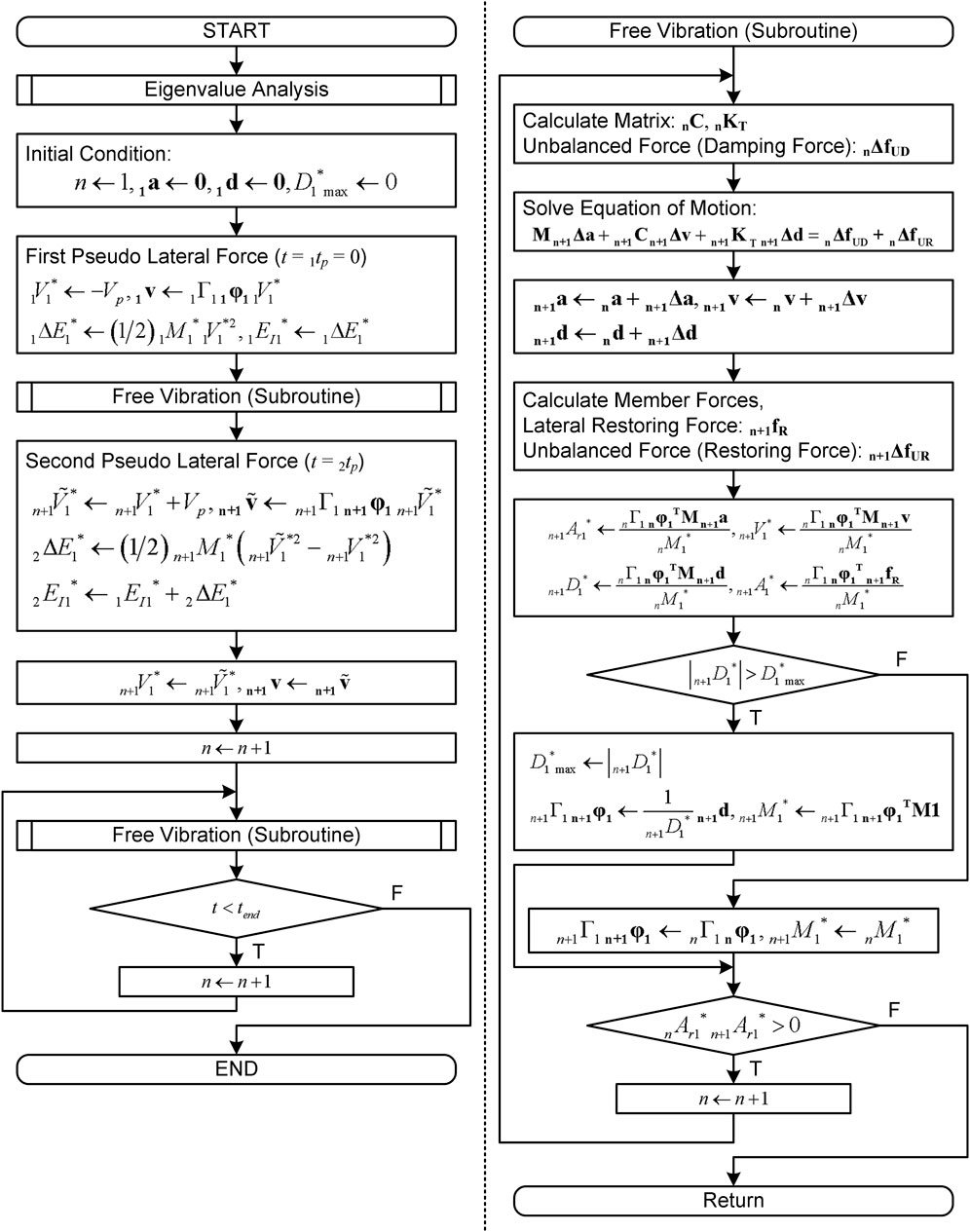
FIGURE 2. Flow of the critical PDI analysis.

When Eq. 39 is satisfied, the second pseudo impulsive lateral force acts.

The analysis procedure was implemented in the computer code used in the previous analysis (Fujii and Miyagawa, 2018).

3 Analysis data and methods

3.1 Building data

The six planar building models analyzed in this study are 8- and 16-story RC MRFs with and without SDCs. Figure 3 shows the simplified plans and elevations of the RC MRF building models. The two models labeled Type B are the same as those used in the previous study (Fujii and Shioda, 2023). Meanwhile, the two models made from the Type B models by removing all SDCs are referred to as Type O. The models referred to as Type A were made from the Type B models by reducing the number of SDCs. All RC MRFs analyzed herein were designed according to the strong-column/weak-beam concept, except for the foundation level beam and in the case of SDCs installed in an RC frame. In the latter case, at the joints between an RC beam and a steel damper column, the RC beam was designed to be sufficiently stronger than the yield strength of the steel damper column considering strain hardening. Sufficient shear reinforcement of all RC members was provided to prevent premature shear failure. The failure of the beam–column joints was not considered because it was assumed that sufficient reinforcement was provided. The natural periods of the first modal response in the elastic range ($T_{1e}$) of the 8-story models are 0.740 s, 0.627 s, and 0.561 s for the Type O, A, and B models, respectively. Similarly, the $T_{1e}$ values of the 16-story models are 1.41 s, 1.21 s, and 1.12 s for the Type O, A, and B models, respectively.

FIGURE 3

FIGURE 3. Simplified structural plans and elevations of the reinforced concrete (RC) moment-resisting frame (MRF) building models.

The nonlinear behavior of the RC members and SDCs was modeled as in previous studies (Mukoyama et al., 2021; Fujii, 2022; Fujii and Shioda, 2023), except for the hysteresis rule used for the SDCs. Figure 4 shows the hysteresis rule. The same hysteresis model (stiffness degradation model) was used for the flexural springs in the RC members. Meanwhile, for the damper panel in the SDCs, two hysteresis models were considered to investigate the influence of strain hardening on the energy response. The first model was the normal bilinear model (LB); its yield strength is set to the initial yielding strength of the damper panel ($Q_{yDL}$), and the strain hardening effect is neglected. The second model was the trilinear model used in previous studies (Mukoyama et al., 2021; Fujii, 2022; Fujii and Shioda, 2023) with the strain-hardening effect (SH); its upper bound strength ($Q_{yDU}$) was set such that the ratio $Q_{yDU}/Q_{yDL}$ equaled 300/205 = 1.46. Other details concerning the six structural models can be found in previous studies (Fujii, 2022; Fujii and Shioda, 2023). In this study, the viscous damping ratio of the first modal response of the RC MRFs in the elastic range ($h_{1f}$) was set to 0.03.

FIGURE 4

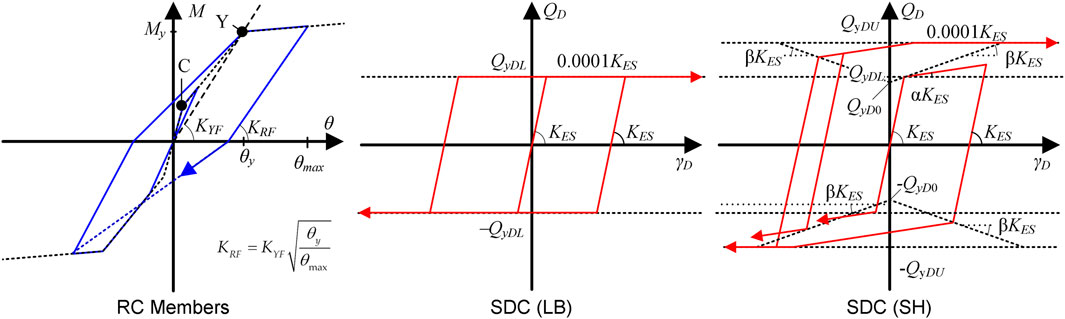
FIGURE 4. Hysteresis model for RC members and steel damper columns (SDCs).

Figure 5 shows the equivalent acceleration–equivalent displacement relationships of the six models. In this study, a displacement-based mode-adaptive pushover (DB-MAP) analysis (Fujii, 2014) was applied to obtain the relationship between the equivalent acceleration (whole building: ${A_1}^{*}$, RC MRF: ${A_{1f}}^{*}$, and SDCs: ${A_{1d}}^{*}$) and the equivalent displacement (${D_1}^{*}$). The pushover analyses were performed until the equivalent displacement (${D_1}^{*}$) reached 1/75 of the assumed equivalent height (${H_1}^{*}$): the assumed ${H_1}^{*}$ values were 18.9 m and 35.9 m for the 8- and 16-story models, respectively. The target equivalent displacement for the pushover analysis was 0.252 m for the 8-story model, while that for the 16-story model was 0.479 m. Note that, in the pushover analyses of the Type A and B models, the influence of the strain hardening of the SDCs was neglected. The idealized ${A_1}^{*}$–${D_1}^{*}$ curves for the Type O models and the idealized ${A_{1f}}^{*}$–${D_1}^{*}$ and ${A_{1d}}^{*}$–${D_1}^{*}$ curves for the Type A and B models are shown in Figure 5. The values of ${D_1}^{*}$ and ${A_1}^{*}$ at the “yield point” ($\left({D_{1yf}}^{*},{A_{1yf}}^{*}\right)$ for RCF and $\left({D_{1yd}}^{*},{A_{1yd}}^{*}\right)$ for SDC) are also shown. The bilinear idealization of each curve was performed following the methods shown in Fujii (2022).

FIGURE 5

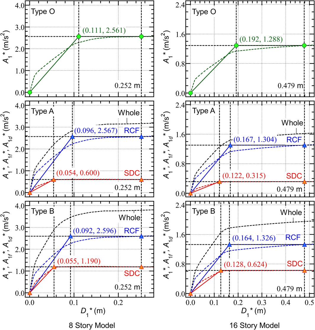
FIGURE 5. Equivalent acceleration–equivalent displacement relationships of the building models.

The following observations can be drawn from Figure 5.

• The “yield displacement” of RCF (${D_{1yf}}^{*}$) in Type A and B models is smaller than that in Type O models. The equivalent drift ratio at the “yielding of RCF” (${D_{1yf}}^{*}/{H_1}^{*}$) of the Type O 8-story model is 1/170, while those of the Type A and B models are 1/196 and 1/205, respectively. Similarly, the ratio ${D_{1yf}}^{*}/{H_1}^{*}$ of the Type O 16-story model is 1/187, while those of the Type A and B models are 1/215 and 1/218, respectively. This is because of the shortening of the beam span resulting from the presence of the SDCs.

• The “yield acceleration” of RCF (${A_{1yf}}^{*}$) in the Type A and B models is nearly the same as that in the Type O models. In case of the 8-story models, the ${A_{1yf}}^{*}$ values of the Type O, A, and B models are 2.561 m/s², 2.567 m/s², and 2.596 m/s², respectively. Similarly, in the case of the 16-story models, the ${A_{1yf}}^{*}$ values of the Type O, A, and B models are 1.288 m/s², 1.304 m/s², and 1.326 m/s², respectively.

• The “yield acceleration” of SDC (${A_{1yd}}^{*}$) in the Type B models is approximately twice of that in the Type A models. The ratio of the “yield acceleration” of SDC to that of RCF (${A_{1yd}}^{*}/{A_{1yf}}^{*}$) of the Type A 8-story model is 0.234, while that of the Type B model is 0.458. Similarly, the ${A_{1yd}}^{*}/{A_{1yf}}^{*}$ ratio of the Type A 16-story model is 0.242, while that of the Type B model is 0.471.

• The ratio of the “yield displacement” of SDC to that of RCF (${D_{1yd}}^{*}/{D_{1yf}}^{*}$) of the 8-story models is smaller than that of the 16-story models. For the 8-story models, the ${D_{1yd}}^{*}/{D_{1yf}}^{*}$ ratios of the Type A and B models are 0.563 and 0.598, respectively. Meanwhile for the 16-story models, the ${D_{1yd}}^{*}/{D_{1yf}}^{*}$ ratios of the Type A and B models are 0.731 and 0.780, respectively.

Note that the ${D_{1yd}}^{*}/{D_{1yf}}^{*}$ ratio influences the effectiveness of the SDCs with respect to seismic energy absorption. This is discussed in the analysis results.

3.2 Analysis method

In this study, the pulse velocity ($V_p$) was set from 0.10 m/s, with an interval of 0.05 m/s, until ${D_1}_{\max }^{*}$ was close to 1/75 of the assumed equivalent height (${H_1}^{*}$). In each analysis, the ending time of the analysis ($t_{end}$) was determined as the ending of the 32nd half cycle of free vibration following the action of the second pseudo impulsive lateral force.

4 Analysis results

In this section, the responses of the building models subjected to a pseudo impulsive lateral force proportional to the first mode vector are compared and discussed. For the Type A and B models, only the results considering strain hardening are shown here.

4.1 Response of the overall building model

Figure 6 compares the relationships between the seismic intensity parameters ($V_p$, ${V_{I1}}^{*}$, and ${V_{\Delta E1}}^{*}$) and the peak equivalent displacement (${D_1}_{\max }^{*}$).

FIGURE 6

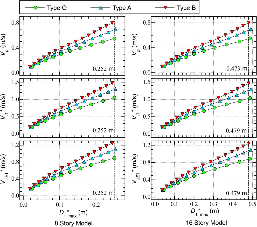
FIGURE 6. Relationship between the seismic intensity parameters and the peak equivalent displacement.

The following conclusions can be drawn from Figure 6.

• The seismic intensity parameters ($V_p$, ${V_{I1}}^{*}$, and ${V_{\Delta E1}}^{*}$) increase as ${D_1}_{\max }^{*}$ increases. The ${V_{I1}}^{*}$–${D_1}_{\max }^{*}$ and ${V_{\Delta E1}}^{*}$–${D_1}_{\max }^{*}$ curves are very similar to the $V_p$–${D_1}_{\max }^{*}$ curve of the same model: the ${V_{I1}}^{*}/V_p$ ratio ranges from 1.8 to 2.0, while the ${V_{\Delta E1}}^{*}/V_p$ ratio ranges from 1.5 to 1.7. The differences in the ${V_{I1}}^{*}/V_p$ and ${V_{\Delta E1}}^{*}/V_p$ ratios between models are very small.

• For the same value of $V_p$, the ${D_1}_{\max }^{*}$ values of the Type B models are the smallest while those of the Type O models are the largest. Comparing the ${D_1}_{\max }^{*}$ values of the 8-story models considering the case where $V_p$ = 0.55 m/s, the ${D_1}_{\max }^{*}$ value for the Type O models is 0.252 m, while those for the Type A and B models are 0.190 m (−24.6%) and 0.162 m (−35.7%), respectively. Similarly, comparing the ${D_1}_{\max }^{*}$ values of the 16-story models considering the case where $V_p$ = 0.55 m/s, the ${D_1}_{\max }^{*}$ value for the Type O models is 0.487 m, while those for the Type A and B models are 0.377 m (−22.6%) and 0.325 m (−33.3%), respectively.

Figure 7 compares the ratios of the cumulative energy at the end of the simulation ($t=t_{end}$), i.e., the ratios of the kinetic energy ($E_K/E_I$), damping dissipated energy ($E_D/E_I$), cumulative strain energy of the RC MRF ($E_{Sf}/E_I$), and cumulative strain energy of the SDCs ($E_{Sd}/E_I$). In this figure, the vertical dotted lines indicate the “yield displacement” of the SDCs (${D_{1yd}}^{*}$) and the RC MRF (${D_{1yf}}^{*}$).

FIGURE 7

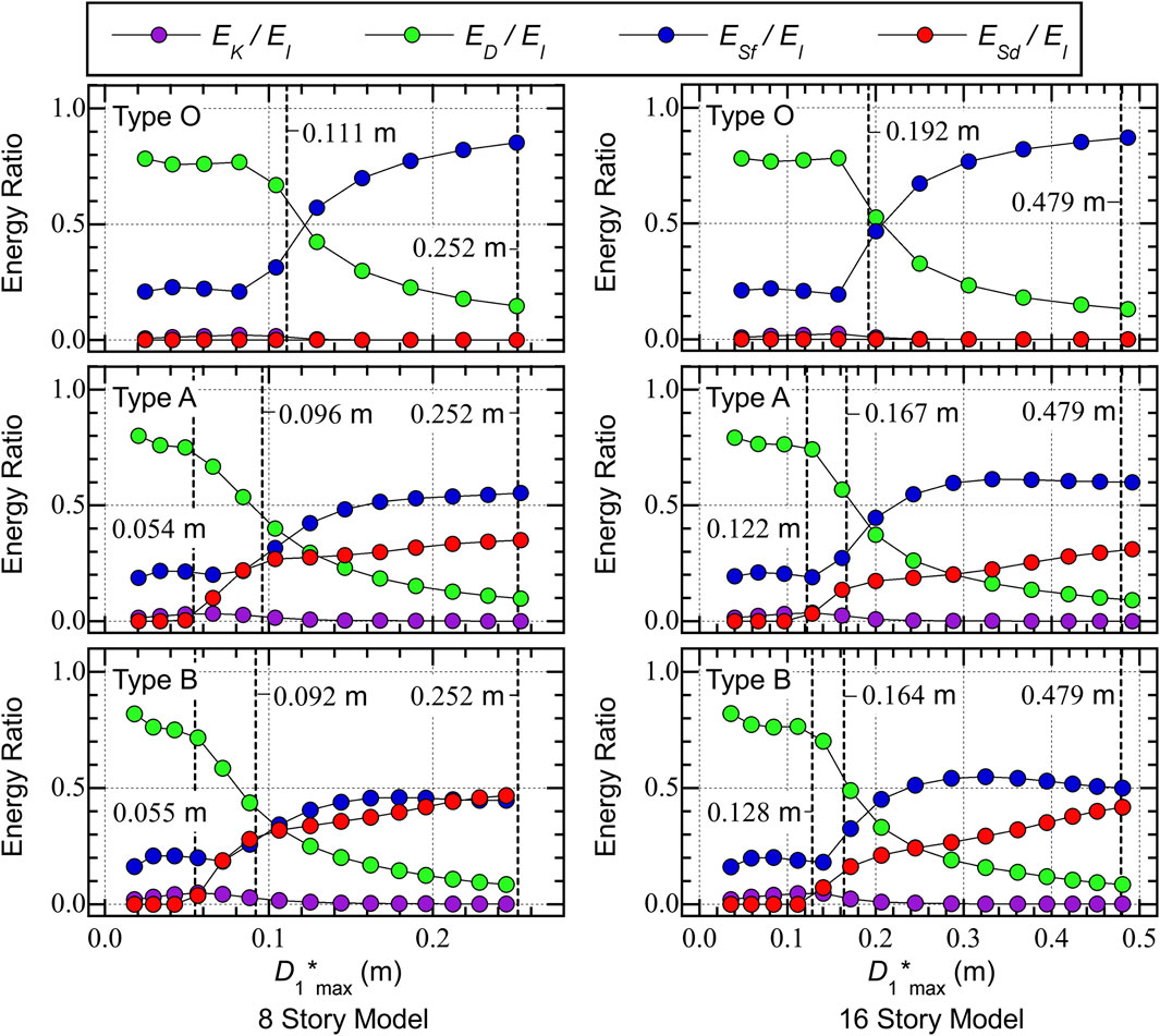
FIGURE 7. Ratios of the cumulative energy at the end of the simulation.

The following conclusions can be drawn from Figure 7.

• In all cases, the ratio of the kinetic energy ($E_K/E_I$) is close to zero.

• For the Type O 8-story model, the $E_D/E_I$ ratio is close to 0.8 when ${D_1}_{\max }^{*}$ is smaller than 0.111 m (= ${D_{1yf}}^{*}$). Meanwhile, the $E_D/E_I$ ratio decreases and the $E_{Sf}/E_I$ ratio increases as ${D_1}_{\max }^{*}$ increases when ${D_1}_{\max }^{*}$ is larger than 0.111 m. When ${D_1}_{\max }^{*}$ is 0.251 m, $E_D/E_I$ is 0.148 while $E_{Sf}/E_I$ is 0.852. Because no SDCs are installed in the Type O models, the $E_{Sd}/E_I$ ratio is zero.

• For the Type A 8-story model, the $E_{Sd}/E_I$ ratio increases as ${D_1}_{\max }^{*}$ increases when ${D_1}_{\max }^{*}$ is larger than 0.054 m (= ${D_{1yd}}^{*}$). The $E_{Sf}/E_I$ ratio increases as ${D_1}_{\max }^{*}$ increases when ${D_1}_{\max }^{*}$ is larger than 0.096 m (= ${D_{1yf}}^{*}$). Meanwhile, the $E_D/E_I$ ratio decreases as ${D_1}_{\max }^{*}$ increases. When ${D_1}_{\max }^{*}$ is 0.254 m, $E_D/E_I$ is 0.097 while $E_{Sf}/E_I$ is 0.553 and $E_{Sd}/E_I$ is 0.350.

• For the Type B 8-story model, similar observations can be made as for the Type A 8-story model. When ${D_1}_{\max }^{*}$ is 0.250 m, $E_D/E_I$ is 0.084 while $E_{Sf}/E_I$ is 0.447 and $E_{Sd}/E_I$ is 0.467.

• For the Type O 16-story model, similar observations can be made as for the Type O 8-story model. When ${D_1}_{\max }^{*}$ is 0.487 m, $E_D/E_I$ is 0.129 while $E_{Sf}/E_I$ is 0.871. Because no SDCs are installed in the Type O models, the $E_{Sd}/E_I$ ratio is zero.

• For the Type A 16-story model, the $E_{Sd}/E_I$ ratio increases as ${D_1}_{\max }^{*}$ increases when ${D_1}_{\max }^{*}$ is larger than 0.122 m (= ${D_{1yd}}^{*}$). The $E_{Sf}/E_I$ ratio increases as ${D_1}_{\max }^{*}$ increases when ${D_1}_{\max }^{*}$ is between 0.167 m (= ${D_{1yf}}^{*}$) and 0.332 m. However, the $E_{Sf}/E_I$ ratio is nearly constant when ${D_1}_{\max }^{*}$ is larger than 0.332 m. When ${D_1}_{\max }^{*}$ is 0.492 m, $E_D/E_I$ is 0.091 while $E_{Sf}/E_I$ is 0.600 and $E_{Sd}/E_I$ is 0.310.

• For the Type B 16-story model, similar observations can be made as for the Type A 16-story model. When ${D_1}_{\max }^{*}$ is 0.480 m, $E_D/E_I$ is 0.084 while $E_{Sf}/E_I$ is 0.499 and $E_{Sd}/E_I$ is 0.417.

The differences in the $E_{Sd}/E_I$ ratios for the 8- and 16-story models can be explained by the differences in the ${D_{1yd}}^{*}/{D_{1yf}}^{*}$ ratios shown in Figure 5. As shown in Figure 5, the ${D_{1yd}}^{*}/{D_{1yf}}^{*}$ ratios in the 8-story models are 0.563 (Type A) and 0.598 (Type B), while those in the 16-story models are 0.731 (Type A) and 0.780 (Type B). Therefore, the effectiveness of the SDCs in 8-story models is better than that in 16-story models because the ${D_{1yd}}^{*}/{D_{1yf}}^{*}$ ratio is smaller for the 8-story models than for the 16-story models.

Figure 8 shows the hysteresis loops of the first modal response (the ${A_1}^{*}\left(t\right)$–${D_1}^{*}\left(t\right)$ relationship) for each model. In this figure, the points at which the first and second pseudo impulsive lateral forces act (${}_1\Delta {E_1}^{*}$ and ${}_2\Delta {E_1}^{*}$, respectively), and the points of the local peak responses (${}_1{D_1}_{peak}^{*}$ and ${}_2{D_1}_{peak}^{*}$, respectively) are shown. The ${A_1}^{*}$–${D_1}^{*}$ curves obtained from the pushover analysis results (as in Figure 5) are also shown Figure 8.

FIGURE 8

FIGURE 8. Hysteresis loop of the first modal response.

The following conclusions can be drawn from Figure 8.

• In all models, larger equivalent displacements occur in the positive direction: $\left|{}_2{D_1}_{peak}^{*}\right|$ is larger than $\left|{}_1{D_1}_{peak}^{*}\right|$. This means that the peak equivalent displacement of the first modal response over the course of the entire seismic event (${D_1}_{\max }^{*}$) occurs at the end of the second half cycle of the response, where the momentary energy input ${}_2\Delta {E_1}^{*}$ occurs.

• For the Type O models (both 8- and 16-story), the ${A_1}^{*}$–${D_1}^{*}$ curves obtained from the pushover analysis results (black dotted curve) agree very well with the hysteresis loops obtained via the critical PDI analyses: the points at the local peak response (${}_1{D_1}_{peak}^{*}$ and ${}_2{D_1}_{peak}^{*}$) are on the ${A_1}^{*}$–${D_1}^{*}$ curves obtained from the pushover analysis results.

• For the Type A and B models (both 8- and 16-story), the ${A_1}^{*}$–${D_1}^{*}$ curves obtained from the pushover analyses are slightly different from the hysteresis loops obtained via the critical PDI analyses: the points at the second local peak response (${}_2{D_1}_{peak}^{*}$) are above the ${A_1}^{*}$–${D_1}^{*}$ curve obtained from the pushover analysis results. For the 8-story models, the ratios of the ${A_1}^{*}$ values obtained from the critical PDI analysis and the pushover analysis at the point ${}_2{D_1}_{peak}^{*}$ are 1.086 for the Type A model and 1.141 for the Type B models. Similary, for the 16-story models, the ratios of the ${A_1}^{*}$ values from the critical PDI analysis and the pushover analysis are 1.083 for the Type A model and 1.149 for the Type B model.

Figure 9 shows the input energy ratio (${\eta }_E$) and the local peak equivalent displacement ratio (${\eta }_D$). Here, the ${\eta }_E$ ratio is defined as Eq. 40:

${\eta }_E={}_1\Delta {E_1}^{*}/{}_2\Delta {E_1}^{*}.(40)$

FIGURE 9

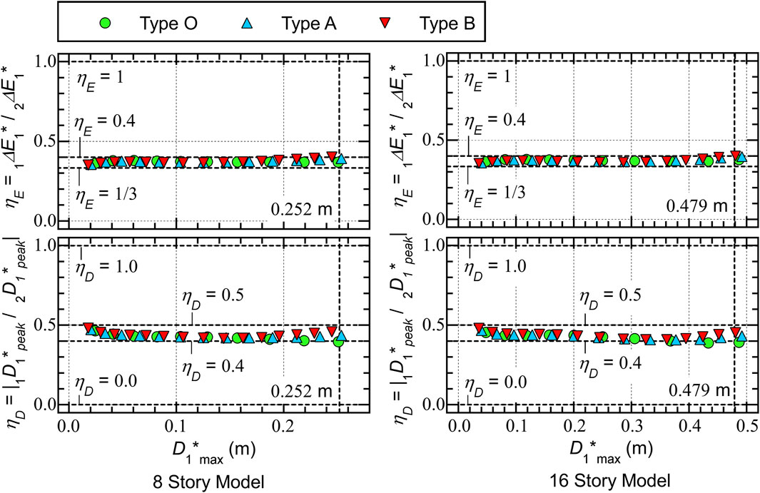
FIGURE 9. Input energy ratio (η_E) and local peak equivalent displacement ratio (η_D).

The ${\eta }_E$ ratio is 1/3 if the structure exhibits undamped linear elastic behavior. Meanwhile, the ${\eta }_E$ ratio is 1 if the structure exhibits rigid–perfectly plastic behavior, that is, no strain energy is released after the first local peak (${}_1{D_1}_{peak}^{*}$) occurs.

The ${\eta }_D$ ratio is defined as Eq. 41:

${\eta }_D=\left|{}_1{D_1}_{peak}^{*}/{}_2{D_1}_{peak}^{*}\right|.(41)$

The ${\eta }_D$ ratio is 0.5 if the structure exhibitis undamped linear elastic behavior. Meanwhile, the ${\eta }_D$ ratio is 1 if the structural response is symmetric in the positive and negative directions.

The following conclusions can be drawn from Figure 9.

• In all models, the ${\eta }_E$ ratio is nearly constant: most of the plots are distributed within a narrow range between 1/3 and 0.4.

• In all models, the ${\eta }_D$ ratio is nearly constant: most of the plots are distributed within a narrow range between 0.4 and 0.5.

Figure 10 shows the response periods of the first modal response ($T_{1res}$) and the ratios of the effective period of the first modal response ($T_{1eff}$) and the response period ($T_{1res}$). Here, $T_{1eff}$ is defined as in Fujii and Shioda (2023) as Eq. 42:

$T_{1eff}=2\pi \sqrt{\frac{4+7\pi \beta }{6}}\frac{{D_1}_{\max }^{*}}{{V_{\Delta E1}}^{*}}.(42)$

FIGURE 10

FIGURE 10. Response period (T_1res).

In Eq. 42, $\beta$ is the complex damping ratio of the equivalent linear system. Here, $\beta$ is set to 0.10.

The following conclusions can be drawn from Figure 10.

• In all models, $T_{1res}$ increases as ${D_1}_{\max }^{*}$ increases.

• When comparing $T_{1res}$ in the case of similar ${D_1}_{\max }^{*}$, $T_{1res}$ of the Type O models is the largest while that of the Type B models is the smallest. This means that $T_{1res}$ becomes smaller as the number of SDCs increases.

• In all models, the $T_{1eff}/T_{1res}$ ratio is nearly constant: all of the plots are distributed within a narrow range between 1.0 and 1.2.

Figure 11 shows the residual equivalent displacement ratio ($r_{resD}$). Here, the $r_{resD}$ ratio is defined as Eq. 43:

$r_{resD}=\left|{D_1}^{*}\left(t_{end}\right)/{D_1}_{\max }^{*}\right|.(43)$

FIGURE 11

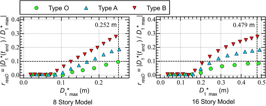
FIGURE 11. Residual equivalent displacement ratio (r_resD).

The following conclusions can be drawn from Figure 11.

• In all models, the $r_{resD}$ ratio increases as ${D_1}_{\max }^{*}$ increases. In all 8-story models, $r_{resD}$ is close to zero when ${D_1}_{\max }^{*}$ is smaller than 0.08 m. Similarly in all 16-story models, $r_{resD}$ is close to zero when ${D_1}_{\max }^{*}$ is smaller than 0.16 m.

• When comparing the ratio $r_{resD}$ in the case of similar ${D_1}_{\max }^{*}$, $r_{resD}$ of the Type O models is the smallest while that of Type B models is the largest. This means that the ratio $r_{resD}$ becomes larger as the number of SDCs increases.

4.2 Local response

Figure 12 compares the peak responses of all model types for $V_p$ = 0.55 m/s. The following local response quantities are compared: 1) the peak relative displacement; 2) the peak story drift; 3) the peak plastic rotation at the beam end (${\theta }_{p\max }$); and 4) the peak shear strain of the damper panel (${\gamma }_{D\max }$). Note that, because the span length is different due to the presence of SDCs, ${\theta }_{p\max }$ for the beam end at the right of column X2 is shown for the Type O and B models; meanwhile, ${\theta }_{p\max }$ for the beam end at the left of column X2 is shown for the Type A models. The plot of ${\gamma }_{D\max }$ for the Type O models is not shown because no SDCs were installed in this model type.

FIGURE 12

FIGURE 12. Comparisons of the peak response (V_p = 0.55 m/s).

The following conclusions can be drawn from Figure 12.

• For both the 8- and 16-story models, the responses of the Type O models are the largest, while those of the Type B models are the smallest.

• For the 8-story models, the largest peak story drift is observed at the third floor level. The largest ${\theta }_{p\max }$ is observed at the third or forth floor levels. The largest ${\gamma }_{D\max }$ is observed at the forth floor level.

• For the 16-story models, the largest peak story drift is observed at the sixth or seventh floor levels. The largest ${\theta }_{p\max }$ is observed at the seventh floor level. The largest ${\gamma }_{D\max }$ is observed at the seventh floor level.

Figure 13 compares the normalized cumulative strain energies of all the model types for $V_p$ = 0.55 m/s. The following local response quantities are compared: 1) the normalized cumulative strain energy at the beam end ($N{E}_{Sb}$) and 2) the normalized cumulative strain energy of the damper panel ($N{E}_{Sd}$). Here, $N{E}_{Sb}$ is defined as Eq. 44:

$N{E}_{Sb,k}=\frac{E_{Sb,k}}{M_{yb,k}\cdot {\theta }_{yb,k}}.(44)$

FIGURE 13

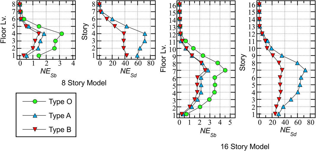
FIGURE 13. Comparisons of the normalized cumulative strain energy (V_p = 0.55 m/s).

In Eq. 44, $M_{yb,k}$ and ${\theta }_{yb,k}$ are the yield moment and the chord rotation, respectively, at the yielding of the $k$ th beam end and $E_{Sb,k}$ is the cumulative strain energy of the $k$ th beam end.

$N{E}_{Sd}$ is defined as Eq. 45:

$N{E}_{Sd,k}=\frac{E_{Sd,k}}{Q_{yDL,k}\cdot {\gamma }_{yDL,k}\cdot h_{d0,k}}.(45)$

In Eq. 45, $Q_{yDL,k}$ and ${\gamma }_{yDL,k}$ are the initial yield shear force and the initial yielding shear strain, respectively, of the $k$ th damper panel; $h_{d0,k}$ is the height of the $k$ th damper panel; and $E_{Sd,k}$ is the cumulative strain energy of the $k$ th damper panel.

The following conclusions can be drawn from Figure 13.

• For both 8- and 16-story models, the $N{E}_{Sb}$ values of the Type O models are the largest, while those of the Type B models are the smallest. The largest $N{E}_{Sb}$ values are observed at the forth floor level in the 8-story models and at the seventh floor level in the 16-story models.

• For both the 8- and 16-story models, the $N{E}_{Sd}$ values of the Type A models are larger than those of the Type B models. In the 8-story models, the largest $N{E}_{Sd}$ is observed at the forth floor level in the Type A models, while it is observed at the first floor level in the Type B models. In the 16-story models, the largest $N{E}_{Sd}$ is observed at the seventh floor level in both model types.

4.3 Summary of the analysis results

This section summarizes the responses of the RC frame building models with and without SDCs subjected to a pseudo impulsive lateral force proportional to the first mode vector. The analysis results can be summarized as follows.

A) In the critical PDI analysis results shown herein, the peak equivalent displacement of the first modal response over the course of the entire seismic event (${D_1}_{\max }^{*}$) occurs at the end of the second half cycle of the response, when the second pseudo impulsive lateral force acts. The momentary input energy corresponding to the second pseudo impulsive lateral force (${}_2\Delta {E_1}^{*}$) is larger than that corresponding to the first pseudo impulsive lateral force (${}_1\Delta {E_1}^{*}$).

B) The equivalent acceleration (${A_1}^{*}$)–equivalent displacement (${D_1}^{*}$) curve obtained from the pushover analysis results agrees very well with the hysteresis loop (the ${A_1}^{*}\left(t\right)$–${D_1}^{*}\left(t\right)$ relationship) obtained by the critical PDI analysis in the case of the Type O models. Meanwhile, in the case of the models with SDCs, the ${A_1}^{*}$–${D_1}^{*}$ curve obtained from the pushover analysis is slightly different from the hysteresis loop obtained by the critical PDI analysis. This is due to the strain hardening effect of the damper panel.

C) The ratio of the effective period of the first modal response ($T_{1eff}$), calculated from Eq. 42, to the response period of the first modal response ($T_{1res}$), $T_{1eff}/T_{1res}$, is nearly constant: the ratio is within a narrow range between 1.0 and 1.2.

D) The ratio of the residual equivalent displacement to the peak equivalent displacement ($r_{resD}$), calculated from Eq. 43, becomes larger as the number of SDCs increases.

Point (A) is important for discussing the relationship between the maximum momentary input energy ($\Delta {E_1}_{\max }^{*}$) and the peak displacement (${D_1}_{\max }^{*}$). In the prediction procedure for the peak displacement of Hori and Inoue (2002), as well as that of Fujii and Shioda (2023), the peak displacement is calculated considering the energy balance during the half cycle of the structural response: it is assumed that the peak displacement (${D_1}_{\max }^{*}$) occurs at the end of the response, when the maximum momentary energy input occurs. Therefore, point (A) is consistent with the assumption of the prediction procedure.

Point (B) indicates that the ${A_1}^{*}$–${D_1}^{*}$ curve obtained from the pushover analysis results agrees well with the critical PDI analysis results, as far as the model without the strain hardening effect is concerned. This implies that, for the bare RC MRF studied herein, the ${A_1}^{*}$–${D_1}^{*}$ curve constructed from the critical PDI analysis results of various $V_p$ by plotting the peak response point will be the same as the ${A_1}^{*}$–${D_1}^{*}$ curve obtained from the pushover analysis.

Point (C) indicates that $T_{1eff}$ calculated from ${D_1}_{\max }^{*}$ and the equivalent velocity of the maximum momentary input energy of the first modal response (${V_{\Delta E1}}^{*}$) via Eq. 42 is clearly related to the response period ($T_{1res}$). This may indicate that Eq. 42 is valid for calculating $T_{1eff}$ when evaluating ${V_{\Delta E1}}^{*}$ and ${V_{I1}}^{*}$ from the $V_{\Delta E}$ and $V_I$ spectra as discussed in previous studies (Fujii, 2023a; Fujii and Shioda, 2023).

Point (D) indicates that the residual displacement after earthquake may be noticeable in case of the large number of SDCs are installed in RC MRFs. One reason why $r_{resD}$ becomes larger as the number of SDCs increases can be explained as follows: the unloading stiffness after the second peak equivalent displacement (${}_2{D_1}_{peak}^{*}$) of Type B is larger than that of Types O and A as shown in Figure 8. This is consistent with the observations pointed out by Ruiz-García (2012b). It should be pointed out that the value of $r_{resD}$ obtained from the critical PDI analysis results is larger than that obtained in the NTHA considering the ground motion records (Fujii, 2022). This is because no seismic input occurs after ${}_2{D_1}_{peak}^{*}$ occurs and the building model oscillates without external forces (free vibration) until $t=t_{end}$ in case of the critical PDI analysis, while in case of the NTHA considering the ground motion records the seismic input continues after the peak response occurs. Therefore, the residual displacement obtained from the critical PDI analysis may be the upper bound.

5 Comparisons with the predicted results

This section focuses on comparisons with the predicted results based on the study of Fujii and Shioda (2023) and the critical PDI analysis results, particularly 1) the ${V_{\Delta E1}}^{*}$–${D_1}^{*}$ relationship and 2) the $T_{1eff}$–${D_1}^{*}$ relationship. Details concerning calculating ${V_{\Delta E1}}^{*}$ and $T_{1eff}$ from the pushover analysis results can be found in Fujii and Shioda (2023).

5.1 Bare RC frame models

Figure 14 shows comparisons between the predicted results and the critical PDI analysis results for the Type O models. The upper two panels show comparisons of the predicted ${V_{\Delta E1}}^{*}$–${D_1}^{*}$ curve and the ${V_{\Delta E1}}^{*}$–${D_1}_{\max }^{*}$ plots obtained from the critical PDI results, while the lower two panels show comparisons of the predicted $T_{1eff}$–${D_1}^{*}$ curve and the $T_{1res}$–${D_1}_{\max }^{*}$ plots obtained from the critical PDI results.

FIGURE 14

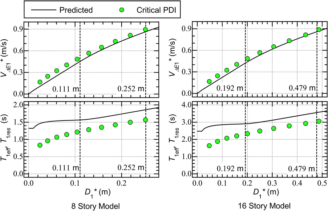
FIGURE 14. Comparisons of the predicted results with the critical PDI analysis results (Type O).

The following conclusions can be drawn from Figure 14.

• The predicted ${V_{\Delta E1}}^{*}$–${D_1}^{*}$ curves are slightly below the ${V_{\Delta E1}}^{*}$–${D_1}_{\max }^{*}$ plots obtained from the critical PDI results. More specifically, the predicted ${V_{\Delta E1}}^{*}$–${D_1}^{*}$ curve of the 8-story model underestimates the critical PDI results when ${D_1}_{\max }^{*}$ is smaller than 0.111 m (= ${D_{1yf}}^{*}$), while the predicted ${V_{\Delta E1}}^{*}$–${D_1}^{*}$ curve becomes closer to the critical PDI results as ${D_1}^{*}$ increases. Similar observations can be made for the 16-story model.

• The predicted $T_{1eff}$–${D_1}^{*}$ curves are above the $T_{1res}$–${D_1}_{\max }^{*}$ plots obtained from the critical PDI results, although its trend is similar. The predicted $T_{1eff}$–${D_1}^{*}$ curves show a gradual increase in $T_{1eff}$ as ${D_1}^{*}$ increases, which is consistent with the $T_{1res}$–${D_1}_{\max }^{*}$ plots. However, the difference between $T_{1eff}$ and $T_{1res}$ becomes significant when ${D_1}_{\max }^{*}$ is small.

5.2 RC frame models with SDCs

Figure 15 shows comparisons between the predicted results and the critical PDI analysis results for the Type A and B models. Similar to Figure 14, the upper two panels show comparisons of the predicted ${V_{\Delta E1}}^{*}$–${D_1}^{*}$ curves with the ${V_{\Delta E1}}^{*}$–${D_1}_{\max }^{*}$ plots obtained from the critical PDI results, while the lower two panels show comparisons of the predicted $T_{1eff}$–${D_1}^{*}$ curves with the $T_{1res}$–${D_1}_{\max }^{*}$ plots obtained from the critical PDI results. In this figure, the critical PDI results obtained by the models without the strain hardening effect (LB) and with the strain hardening effect (SH) are shown for comparison.

FIGURE 15

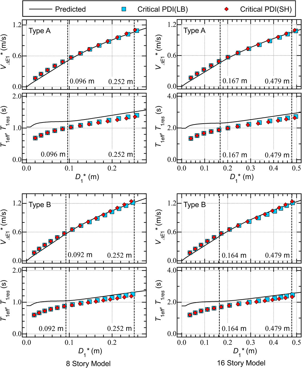
FIGURE 15. Comparisons of the predicted results with the critical PDI analysis results (Types A and B).

The following conclusions can be drawn from Figure 15.

• As far as the ${V_{\Delta E1}}^{*}$–${D_1}_{\max }^{*}$ and $T_{1res}$–${D_1}_{\max }^{*}$ plots are concerned, the differences between the LB (without strain hardening) and SH (with strain hardening) plots are very small in the critical PDI analysis results shown herein.

• The predicted ${V_{\Delta E1}}^{*}$–${D_1}^{*}$ curves agree well with the ${V_{\Delta E1}}^{*}$–${D_1}_{\max }^{*}$ plots obtained from the critical PDI results for all models shown herein.

• The predicted $T_{1eff}$–${D_1}^{*}$ curves are above the $T_{1res}$–${D_1}_{\max }^{*}$ plots obtained from the critical PDI results, and the difference between the predicted $T_{1eff}$–${D_1}^{*}$ curves and the $T_{1res}$–${D_1}_{\max }^{*}$ plots decreases as ${D_1}^{*}$ increases.

5.3 Discussion

This section compares the predicted results based on the study of Fujii and Shioda (2023) with the critical PDI analysis results, focusing on 1) comparisons between the predicted ${V_{\Delta E1}}^{*}$–${D_1}^{*}$ curves and the ${V_{\Delta E1}}^{*}$–${D_1}_{\max }^{*}$ plots obtained from the critical PDI results and 2) comparisons between the predicted $T_{1eff}$–${D_1}^{*}$ curves and the $T_{1res}$–${D_1}_{\max }^{*}$ plots. Based on these comparisons, the following conclusions can be drawn.

A) The predicted ${V_{\Delta E1}}^{*}$–${D_1}^{*}$ curves are slightly below the ${V_{\Delta E1}}^{*}$–${D_1}_{\max }^{*}$ plots obtained from the critical PDI results for bare RC MRF models. Meanwhile, the predicted ${V_{\Delta E1}}^{*}$–${D_1}^{*}$ curves agree well with the ${V_{\Delta E1}}^{*}$–${D_1}_{\max }^{*}$ plots obtained from the critical PDI results for RC MRF models with SDCs shown herein.

B) The predicted $T_{1eff}$–${D_1}^{*}$ curves are slightly above the $T_{1res}$–${D_1}_{\max }^{*}$ plots obtained from the critical PDI results. Although their trends are similar, the predicted $T_{1eff}$–${D_1}^{*}$ curves show a gradual increase in $T_{1eff}$ as ${D_1}^{*}$ increases, which is consistent with the $T_{1res}$–${D_1}_{\max }^{*}$ plots. The difference between the predicted $T_{1eff}$–${D_1}^{*}$ curve and the $T_{1res}$–${D_1}_{\max }^{*}$ plots is noticeable for the bare RC MRF models, while the difference is much smaller for the RC MRF models with SDCs.

C) The influence of the strain hardening of the damper panels on the ${V_{\Delta E1}}^{*}$–${D_1}_{\max }^{*}$ and $T_{1res}$–${D_1}_{\max }^{*}$ plots of the RC MRF models with SDCs is negligibly small.

Conclusion (A) indicates that the accuracy of the predicted ${V_{\Delta E1}}^{*}$–${D_1}^{*}$ curves is satisfactory, as far as the bare RC MRF models and RC MRF models with SDCs are concerned. However, the difference between the predicted $T_{1eff}$ and $T_{1res}$ is not small when ${D_1}_{\max }^{*}$ is small, as evident in conclusion (B). There are two main reasons why the difference between the predicted $T_{1eff}$ and $T_{1res}$ is larger for the bare RC MRF models than the RC MRF models with SDCs. The first is the difference of accuracy of the predicted ${V_{\Delta E1}}^{*}$–${D_1}^{*}$ curve. As shown in Eq. 42, the predicted $T_{1eff}$ is a function of the secant slope of the predicted ${V_{\Delta E1}}^{*}$–${D_1}^{*}$ curve (${V_{\Delta E1}}^{*}/{D_1}^{*}$): the predicted $T_{1eff}$ is larger when the predicted ${V_{\Delta E1}}^{*}$–${D_1}^{*}$ curve is conservative. Note that in this study the skeleton curve of the all RC members are modeled as tri-linear curve as shown in Figure 4, while for the calculation of ${V_{\Delta E1}}^{*}$–${D_1}^{*}$ curve, the idealization of the ${A_{1f}}^{*}$–${D_1}^{*}$ curve is made via a bi-linear curve. This bi-linear idealization of the ${A_{1f}}^{*}$–${D_1}^{*}$ curve is one of the sources of conservativeness of ${V_{\Delta E1}}^{*}$–${D_1}^{*}$ curve. Because most of the energy input during a half cycle of structural response is absorbed as the hysteretic dissipated energy of RC MRF in case of the bare RC MRF models, the influence of bi-linear idealization of the ${A_{1f}}^{*}$–${D_1}^{*}$ curve to the accuracy of the predicted ${V_{\Delta E1}}^{*}$–${D_1}^{*}$ curve is more noticeable in case of the bare RC MRF models than in case of RC MRF models with SDCs. The second reason is the assumed value of the complex damping ratio of the equivalent linear system ($\beta$) in Eq. 42. In this study, $\beta$ was set 0.10 based on the results obtained in previous work by the author using the RC MRF models with SDCs (Fujii and Shioda, 2023). The hysteretic dissipated energy of the bare RC MRF model is smaller than the RC MRF models with SDCs due to the absence of SDCs. Therefore, the value $\beta$ = 0.10 may be too large for the bare RC MRF models, even though the value $\beta$ = 0.10 is suitable for the RC MRF models with SDCs. Conclusion (C) indicates that the strain hardening effect of the damper panel can be neglected in calculations of the ${V_{\Delta E1}}^{*}$–${D_1}^{*}$ curve.

6 Conclusion

In this study, critical PDI analyses of six RC MRF models with and without SDCs were performed. Then, the predicted ${V_{\Delta E1}}^{*}$–${D_1}^{*}$ and ${T_1}_{eff}$–${D_1}^{*}$ relationships calculated according to Fujii and Shioda (2023) were compared with those obtained from the critical PDI analysis results. The main results and conclusions can be summarized as follows.

• The equivalent acceleration (${A_1}^{*}$)–equivalent displacement (${D_1}^{*}$) curves obtained from the pushover analysis results agree very well with the hysteresis loops (${A_1}^{*}\left(t\right)$–${D_1}^{*}\left(t\right)$ relationship) obtained by the critical PDI analysis in the case of models without SDCs. In the case of models with SDCs, the ${A_1}^{*}$–${D_1}^{*}$ curve obtained from the pushover analysis differs slightly from the hysteresis loop obtained by the critical PDI analysis.

• The effective period of the first modal response ($T_{1eff}$), calculated from the equation of the peak equivalent displacement (${D_1}_{\max }^{*}$) and the equivalent velocity of the maximum momentary input energy (${V_{\Delta E1}}^{*}$), is clearly related to the response period ($T_{1res}$); the $T_{1eff}/T_{1res}$ ratio is within a narrow range between 1.0 and 1.2.

• The predicted ${V_{\Delta E1}}^{*}$–${D_1}^{*}$ curves are slightly below the ${V_{\Delta E1}}^{*}$–${D_1}_{\max }^{*}$ plots obtained from the critical PDI results for bare RC MRF models. In addition, the predicted ${V_{\Delta E1}}^{*}$–${D_1}^{*}$ curves agree well with the ${V_{\Delta E1}}^{*}$–${D_1}_{\max }^{*}$ plots obtained from the critical PDI results for RC MRF models with SDCs shown herein. Meanwhile, the predicted $T_{1eff}$–${D_1}^{*}$ curves are slightly above the $T_{1res}$–${D_1}_{\max }^{*}$ plots obtained from the critical PDI results. Although their trends are similar, the predicted $T_{1eff}$–${D_1}^{*}$ curves show a gradual increase in $T_{1eff}$ as ${D_1}^{*}$ increases, which is consistent with the $T_{1res}$–${D_1}_{\max }^{*}$ plots.

• The influence of the strain hardening of the damper panels on the ${V_{\Delta E1}}^{*}$–${D_1}_{\max }^{*}$ and $T_{1res}$–${D_1}_{\max }^{*}$ plots of the RC MRF models with SDCs is negligibly small.

The above conclusions support the accuracy of the prediction procedure (Fujii and Shioda, 2023): the predicted ${V_{\Delta E1}}^{*}$–${D_1}^{*}$ curves are sufficiently accurate for RC MRFs with and without SDCs. In addition, considering the unavoidable scatter in evaluating ${V_{\Delta E1}}^{*}$ and ${V_{I1}}^{*}$ from the linear spectrum, the accuracy of the predicted $T_{1eff}$–${D_1}^{*}$ curves may be acceptable.

Another finding of interest is that the ${V_{\Delta E1}}^{*}$–${D_1}^{*}$ curve can be directly evaluated from the critical PDI (or PMI) analysis in the case of buildings with a significant cyclic loading effect. In the DB-MAP analysis, there are several limitations imposed to avoid instability problems in the numerical analysis, e. g., the envelope of the force–deformation relationship of members must be symmetric, and a severe strength degradation (severe negative slope) in the force–deformation relationship of brittle members may cause numerical stability. In addition, because the DB-MAP analysis is a monotonic loading analysis, the influence of the cyclic loading effect cannot be directly included. Meanwhile, the critical PDI analysis shown herein has no such limitations; a critical PDI analysis of a structural model can be performed as long as the structural model is stable for NTHA. The flow of the critical PDI analysis shown herein can easily be extended to a critical PMI analysis. Therefore, the influence of the number of cyclic loadings on the ${V_{\Delta E1}}^{*}$–${D_1}^{*}$ curve can easily be evaluated by increasing the number of impulsive inputs in the critical PMI analysis. Therefore, critical PDI analyses have great potential for seismic performance evaluations of structures.

Note that the results shown in this study are, so far, valid only for RC MRF models with and without SDCs. Therefore, apart from further verifications using additional building models, the following questions remain unanswered. This list of questions is not comprehensive.

• What is the dependence of the ${V_{\Delta E1}}^{*}$–${D_1}^{*}$ curve on the number of impulsive inputs? It is expected that the ratio of the amplitude of ${D_1}^{*}$ in the positive and negative directions changes as the number of impulsive inputs increases. Therefore, the relationship between the increment of the energy input in each half cycle and the local peak equivalent displacement should vary depending on the number of impulsive inputs.

• Can the distribution of the cumulative strain energy of the SDCs in the critical PDI analysis at each floor level be properly evaluated from the pushover analysis results? Because the pushover analysis cannot consider the strain hardening effect, the distribution of the deformation of the SDCs may be different from the critical PDI analysis results. It is expected that the influence of the strain hardening effect on the distribution of the cumulative strain energy of the SDCs may be significant when the number of impulsive inputs increases.

Data availability statement

The raw data supporting the conclusion of this article will be made available by the authors, without undue reservation.

Author contributions

KF: Writing–original draft, Writing–review and editing.

Funding

The author(s) declare financial support was received for the research, authorship, and/or publication of this article. This study received financial support from JSPS KAKENHI Grant Number JP23K41046.

Acknowledgments

The original frame model data used in this study were provided by Momoka Shioda, who is a former graduate student of the Chiba Institute of Technology. We thank Martha Evonuk, PhD, from Edanz (https://jp.edanz.com/ac), for editing a draft of this manuscript.

Conflict of interest

The author declares that the research was conducted in the absence of any commercial or financial relationships that could be construed as a potential conflict of interest.

Publisher’s note

All claims expressed in this article are solely those of the authors and do not necessarily represent those of their affiliated organizations, or those of the publisher, the editors and the reviewers. Any product that may be evaluated in this article, or claim that may be made by its manufacturer, is not guaranteed or endorsed by the publisher.

Abbreviations

DB-MAP, displacement-based mode-adaptive pushover; MDOF, multi-degree-of-freedom; MRF, moment-resisting frame; NTHA, nonlinear time-history analysis; PDI, pseudo-double impulse; RC, reinforced concrete; SDC, steel damper column; SDOF, single-degree-of-freedom.

References

Akehashi, H., and Takewaki, I. (2021). Pseudo-double impulse for simulating critical response of elastic-plastic MDOF model under near-fault earthquake ground motion. Soil Dyn. Earthq. Eng. 150, 106887. doi:10.1016/j.soildyn.2021.106887

CrossRef Full Text | Google Scholar

Akehashi, H., and Takewaki, I. (2022). Pseudo-multi impulse for simulating critical response of elastic-plastic high-rise buildings under long-duration, long-period ground motion. Struct. Des. Tall Special Build. 31 (14), e1969. doi:10.1002/tal.1969

CrossRef Full Text | Google Scholar

Akiyama, H. (1985). Earthquake resistant limit-state design for buildings. Tokyo: University of Tokyo Press.

Google Scholar

Akiyama, H. (1988). “Earthquake resistant design based on the energy concept,” in Proceedings of the 9th World Conference on Earthquake Engineering, Tokyo-Kyoto, Japan.

Google Scholar

Akiyama, H. (1999). Earthquake-resistant design method for buildings based on energy balance. Tokyo: Gihodo Shuppan.

Google Scholar

Angelucci, G., Mollaioli, F., and Quaranta, G. (2023b). Correlation between energy and displacement demands for infilled reinforced concrete frames. Front. Built Environ. 9, 1198478. doi:10.3389/fbuil.2023.1198478

CrossRef Full Text | Google Scholar

Angelucci, G., Quaranta, G., Mollaioli, F., and Kunnath, S. K. (2023a). “Correlation between seismic energy demand and damage potential under pulse-like ground motions,” in Energy-based seismic engineering. IWEBSE 2023. Lecture notes in civil engineering. Editors H. Varum, A. Benavent-Climent, and F. Mollaioli (Cham: Springer), Vol. 236.

CrossRef Full Text | Google Scholar

Benavent-Climent, A. (2011). A seismic index method for vulnerability assessment of existing frames: application to RC structures with wide beams in Spain. Bull. Earthq. Eng. 9, 491–517. doi:10.1007/s10518-010-9200-z

CrossRef Full Text | Google Scholar

Benavent-Climent, A., Akiyama, H., López-Almansa, F., and Pujades, L. G. (2004). Prediction of ultimate earthquake resistance of gravity-load designed RC buildings. Eng. Struct. 26, 1103–1113. doi:10.1016/j.engstruct.2004.03.011

CrossRef Full Text | Google Scholar

Decanini, L., Mollaioli, F., and Saragoni, R. (2000). “Energy and displacement demands imposed by near-source ground motions,” in Proceedings of the 12th World Conference on Earthquake Engineering, Auckland, New Zealand.

Google Scholar

Elwood, K. J., Sarrafzadeh, M., Pujol, S., Liel, A., Murray, P., Shah, P., et al. (2021). “Impact of prior shaking on earthquake response and repair requirements for structures—studies from ATC-145,” in Proceedings of the NZSEE 2021 Annual Conference, Christchurch, New Zealand.

Google Scholar

Fajfar, P. (1992). Equivalent ductility factors, taking into account low-cycle fatigue. Earthq. Eng. Struct. Dyn. 21, 837–848. doi:10.1002/eqe.4290211001

CrossRef Full Text | Google Scholar

Fajfar, P., and Gaspersic, P. (1996). The N2 method for the seismic damage analysis of RC buildings. Earthq. Eng. Struct. Dyn. 25, 31–46. doi:10.1002/(sici)1096-9845(199601)25:1<31::aid-eqe534>3.0.co;2-v

CrossRef Full Text | Google Scholar

Farrow, K. T., and Kurama, Y. C. (2003). SDOF demand index relationships for performance-based seismic design. Earthq. Spectra 19 (4), 799–838. doi:10.1193/1.1622955

CrossRef Full Text | Google Scholar

Fujii, K. (2014). Prediction of the largest peak nonlinear seismic response of asymmetric buildings under bi-directional excitation using pushover analyses. Bull. Earthq. Eng. 12, 909–938. doi:10.1007/s10518-013-9557-x

CrossRef Full Text | Google Scholar

Fujii, K. (2021). Bidirectional seismic energy input to an isotropic nonlinear one-mass two-degree-of-freedom system. Buildings 11, 143. doi:10.3390/buildings11040143

CrossRef Full Text | Google Scholar

Fujii, K. (2022). Peak and cumulative response of reinforced concrete frames with steel damper columns under seismic sequences. Buildings 12, 275. doi:10.3390/buildings12030275

CrossRef Full Text | Google Scholar

Fujii, K. (2023a). Energy-based response prediction of reinforced concrete buildings with steel damper columns under pulse-like ground motions. Front. Built Environ. 9, 1219740. doi:10.3389/fbuil.2023.1219740

CrossRef Full Text | Google Scholar

Fujii, K. (2023b). “Equivalent number of cycles formulation for a base-isolated building,” in Energy-based seismic engineering. IWEBSE 2023. Lecture notes in civil engineering. Editors H. Varum, A. Benavent-Climent, and F. Mollaioli (Cham: Springer), Vol. 236.

CrossRef Full Text | Google Scholar

Fujii, K., Kanno, H., and Nishida, T. (2019b). Formulation of the time-varying function of momentary energy input to a SDOF system by Fourier series. J. Jpn. Assoc. Earthq. Eng. 19, 247–255. doi:10.5610/jaee.19.5_247

CrossRef Full Text | Google Scholar

Fujii, K., Kanno, H., and Nishida, T. (2021). “Prediction of the peak displacement of the reinforced concrete structure with brittle members based on the momentary energy input,” in Proceedings of the 17th World Conference on Earthquake Engineering, Sendai, Japan.

Google Scholar

Fujii, K., and Miyagawa, K. (2018). “Nonlinear seismic response of a seven-story steel reinforced concrete condominium retrofitted with low-yield-strength-steel damper columns,” in Proceedings of the 16th European Conference on Earthquake Engineering (Thessaloniki).

Google Scholar

Fujii, K., and Murakami, Y. (2021). “Bidirectional momentary energy input to a one-mass two-DOF system,” in Proceedings of the 17th World Conference on Earthquake Engineering, Sendai, Japan.

Google Scholar

Fujii, K., and Shioda, M. (2023). Energy-based prediction of the peak and cumulative response of a reinforced concrete building with steel damper columns. Buildings 13, 401. doi:10.3390/buildings13020401

CrossRef Full Text | Google Scholar

Fujii, K., Sugiyama, H., and Miyagawa, K. (2019a). Predicting the peak seismic response of a retrofitted nine-storey steel reinforced concrete building with steel damper columns. Earthquake Resistant Engineering Structures XII. WIT Trans. Built Environ. 185, PII75–85. doi:10.2495/ERES190061

CrossRef Full Text | Google Scholar

Gaspersic, P., Fajfar, P., and Fischinger, M. (1992). “An approximate method for seismic damage analysis of buildings,” in Proceedings of the 10th World Conference on Earthquake Engineering, Madrid, Spain.

Google Scholar

Hori, N., and Inoue, N. (2002). Damaging properties of ground motions and prediction of maximum response of structures based on momentary energy response. Earthq. Eng. Struct. Dyn. 31, 1657–1679. doi:10.1002/eqe.183

CrossRef Full Text | Google Scholar

Hori, N., Iwasaki, T., and Inoue, N.(2000). “Damaging properties of ground motions and response behavior of structures based on momentary energy response,” in Proceedings of the 12th World Conference on Earthquake Engineering, Auckland, New Zealand.

Google Scholar

Hoveidae, N., and Radpour, S. (2021). Performance evaluation of buckling-restrained braced frames under repeated earthquakes. Bull. Earthq. Eng. 19, 241–262. doi:10.1007/s10518-020-00983-0

CrossRef Full Text | Google Scholar

Inoue, N., Wenliuhan, H., Kanno, H., Hori, N., and Ogawa, J. (2000). “Shaking table tests of reinforced concrete columns subjected to simulated input motions with different time durations,” in Proceedings of the 12th World Conference on Earthquake Engineering, Auckland, New Zealand.

Google Scholar

Kalkan, E., and Kunnath, S. K. (2007). Effective cyclic energy as a measure of seismic demand. J. Earthq. Eng. 11 (5), 725–751. doi:10.1080/13632460601033827

CrossRef Full Text | Google Scholar

Katayama, T., Ito, S., Kamura, H., Ueki, T., and Okamoto, H.(2000). “Experimental study on hysteretic damper with low yield strength steel under dynamic loading,” in Proceedings of the 12th World Conference on Earthquake Engineering, Auckland, New Zealand.

Google Scholar

Kojima, K., Fujita, K., and Takewaki, I. (2015). Critical double impulse input and bound of earthquake input energy to building structure. Front. Built Environ. 1, 5. doi:10.3389/fbuil.2015.00005

CrossRef Full Text | Google Scholar

Kojima, K., and Takewaki, I. (2015a). Critical earthquake response of elastic–plastic structures under near-fault ground motions (Part 1: fling-step input). Front. Built Environ. 1, 12. doi:10.3389/fbuil.2015.00012

CrossRef Full Text | Google Scholar

Kojima, K., and Takewaki, I. (2015b). Critical earthquake response of elastic–plastic structures under near-fault ground motions (Part 2: forward-directivity input). Front. Built Environ. 1, 13. doi:10.3389/fbuil.2015.00013

CrossRef Full Text | Google Scholar

Kojima, K., and Takewaki, I. (2015c). Critical input and response of elastic–plastic structures under long-duration earthquake ground motions. Front. Built Environ. 1, 15. doi:10.3389/fbuil.2015.00015

CrossRef Full Text | Google Scholar

Manfredi, G. M., and Cosenza, E. (2003). Cumulative demand of the earthquake ground motions in the near source. Earthq. Eng. Struct. Dyn. 32, 1853–1865. doi:10.1002/eqe.305

CrossRef Full Text | Google Scholar

McCormick, J., Des Roches, R., Fugazza, D., and Auricchio, F. (2007). Seismic assessment of concentrically braced steel frames with shape memory alloy braces. J. Struct. Eng. ASCE 133 (6), 862–870. doi:10.1061/(asce)0733-9445(2007)133:6(862)

CrossRef Full Text | Google Scholar

Mollaioli, F., Bruno, S., Decanini, L., and Saragoni, R. (2011). Correlations between energy and displacement demands for performance-based seismic engineering. Pure Appl. Geophys. 168, 237–259. doi:10.1007/s00024-010-0118-9

CrossRef Full Text | Google Scholar

Mota-Páez, S., Escolano-Margarit, D., and Benavent-Climent, A. (2021). Seismic response of RC frames with a soft first story retrofitted with hysteretic dampers under near-fault earthquakes. Appl. Sci. 11, 1290. doi:10.3390/app11031290

CrossRef Full Text | Google Scholar

Mukoyama, R., Fujii, K., Irie, C., Tobari, R., Yoshinaga, M., and Miyagawa, K. (2021). “Displacement-controlled seismic design method of reinforced concrete frame with steel damper column,” in Proceedings of the 17th World Conference on Earthquake Engineering, Sendai, Japan.

Google Scholar

Nakashima, M. (1995). Strain-hardening behavior of shear panels made of low-yield steel. I: test. J. Struct. Eng. ASCE 121 (12), 1742–1749. doi:10.1061/(asce)0733-9445(1995)121:12(1742)

CrossRef Full Text | Google Scholar

Ruiz-García, J. (2012a). Mainshock-aftershock ground motion features and their influence in building's seismic response. J. Earthq. Eng. 16 (5), 719–737. doi:10.1080/13632469.2012.663154

CrossRef Full Text | Google Scholar

Ruiz-García, J. (2012b). “Issues on the response of existing buildings under mainshock-aftershock seismic sequences,” in Proceedings of the 15th World Conference on Earthquake Engineering, Lisbon, Portugal.

Google Scholar

Ruiz-García, J., and Negrete-Manriquez, J. C. (2011). Evaluation of drift demands in existing steel frames under as-recorded far-field and near-fault mainshock–aftershock seismic sequences. Eng. Struct. 33, 621–634. doi:10.1016/j.engstruct.2010.11.021

CrossRef Full Text | Google Scholar

Teran-Gilmore, A. (1998). A parametric approach to performance-based numerical seismic design. Earthq. Spectra 14 (3), 501–520. doi:10.1193/1.1586012

CrossRef Full Text | Google Scholar

Tesfamariam, S., and Goda, K. (2015). Seismic performance evaluation framework considering maximum and residual inter-story drift ratios: application to non-code conforming reinforced concrete buildings in Victoria, BC, Canada. Front. Built Environ. 1, 18. doi:10.3389/fbuil.2015.00018

CrossRef Full Text | Google Scholar

Tremblay, R., Lacerte, M., and Christopoulos, C. (2008). Seismic response of multistory buildings with self-centering energy dissipative steel braces. J. Struct. Eng. ASCE 134 (1), 108–120. doi:10.1061/(asce)0733-9445(2008)134:1(108)

CrossRef Full Text | Google Scholar

Wada, A., Huang, Y. H., and Iwata, M. (2000). Passive damping technology for buildings in Japan. Prog. Struct. Eng. Mater. 2 (3), 335–350. doi:10.1002/1528-2716(200007/09)2:3<335::aid-pse40>3.0.co;2-a

CrossRef Full Text | Google Scholar