Evaluation of data-driven NARX model based compensation for multi-axial real-time hybrid simulation benchmark study

1 Introduction

Experimental technique plays an indispensable role in advancing earthquake engineering research. Rigorous experimentation is crucial for new structures or materials to be considered suitable for engineering applications. In comparison with conventional methods such as shaking table tests and quasi-static tests, real-time hybrid simulation (RTHS) stands out by integrating numerical modeling of analytical substructures with physical testing of experimental substructures. This integration allows full scale test possible in both time and size. With over 2 decades of dedicated research focusing on integration algorithms, delay compensation, and evaluation methods, RTHS has emerged as an effective and efficient technique for performance evaluation of systems under earthquakes. Its capability to facilitate real-time, large-scale testing has significantly contributed to the evaluation and validation of technologies for seismic hazard mitigation, marking a pivotal milestone in the field of earthquake engineering (Nakashima et al., 1992; Ou et al., 2015; Tian et al., 2020; Li et al., 2022; Palacio-Betancur and Soto, 2023).

RTHS can be categorized based on the number of experimental substructures or actuators required as single-actuator RTHS (saRTHS) or multiple-actuator or multi-axial RTHS (maRTHS) (Chen and Ricles, 2012; Lu et al., 2022; Najafi et al., 2023). In saRTHS, a solitary actuator is employed to apply the desired displacement exclusively to the only experimental substructure. Conversely, maRTHS demands a minimum of two hydraulic actuators to impart the necessary motion to experimental substructures. In the context of saRTHS, the implementation of single-input single-output (SISO) control is imperative to mitigate actuator delay introduced by actuator dynamics. Previous research underscores that actuator delay can be regarded as equivalent to negative damping, leading to inaccuracies in test results and even destabilize the overall simulation if not compensated adequately (Horiuchi et al., 1999; Wallace et al., 2005; Chen and Ricles, 2008). Traditional delay compensation methods typically require researchers to pre-estimate the time delay before conducting tests, assuming constant delay or constant actuator dynamics throughout RTHS. Consequently, the efficacy of such methods heavily relies on the accuracy of this estimation (Carrion and Spencer, 2008). However, researchers have also noted that actuator dynamics are frequency-dependent and time-varying. This suggests that signals with varying frequencies or times may correspond to different actuator delays. Consequently, both the assumption of constant delay and constant actuator dynamics are inconsistent with the actual actuator dynamics, even when actuator delay or dynamics are accurately predicted (Xu et al., 2016).

To address the limitations of traditional compensations, adaptive methods utilize measured displacements from actuators to continually update estimations during RTHS, enhancing compensation performance. These approaches are often termed adaptive compensation methods, as their parameters undergo self-regulation. Consequently, the need for accurately estimating actuator delay or dynamics before tests is eliminated. Furthermore, the adaptive nature of these methods allows for the regulation of time-varying delays or actuator dynamics. As a result, adaptive compensation methods have become the predominant approach in RTHS, with many validated through benchmark problems (Ning et al., 2019; Wang et al., 2019; Xu et al., 2019; Zhou et al., 2019; Silva et al., 2020). Among these methods, the Nonlinear Autoregressive with External Input Model (NARX) compensation (Xu et al., 2022)constructs the actuator dynamics as a function of previously predicted displacements and current or previous measured displacements. The relationship between calculated displacement and predicted displacement is determined based on this actuator dynamics model. NARX model-based compensation can be further categorized into different orders, such as first order NARX (F-NARX), second order NARX (S-NARX), third order NARX (T-NARX), and higher order NARX, depending on the number of previous calculated displacements considered in the formulation. When nonlinear terms are ignored, NARX degenerates into autoregressive with external input (ARX). This is akin to adaptive time series compensation (ATS) (Chae et al., 2013) when the ordinary least squares method is applied to compute coefficients in the NARX model (Chae et al., 2013; Chae et al., 2013). Furthermore, first order NARX can be considered as an adaptive alternative to traditional inverse compensation (Chen and Ricles, 2008).

In contrast with saRTHS, maRTHS offers the advantage of synergistically utilizing existing laboratory facilities to address multi-dimensional problems, thus presenting potential solutions to complex engineering challenges. However, the transition to maRTHS requires the adoption of multiple-input multiple-output (MIMO) control strategies instead of single-input single-output (SISO) control, thus imposing challenges. Moreover, the global performance of saRTHS mainly depends on the tracking performance of one actuator, while tracking performance of all actuators should be considered for maRTHS.

In this study, data-driven NARX model-based compensation is evaluated for the maRTHS benchmark model (Uribe et al., 2023), which features a steel frame, two hydraulic actuators, and a high-stiffness steel coupler. Expanding upon the groundwork laid by the NARX controller proposed by Xu et al. (2022), this study delves into the integration of nonlinear terms into the NARX model-based compensation framework. Whereas previous applications primarily focused on linear terms, this research introduces the inclusion of nonlinear elements for enhanced practical implementation. Moreover, the study advocates for the utilization of ridge regression techniques to bolster the efficacy of online least square regression within the NARX framework. Ten criteria are utilized to evaluate the performance of RTHS including both tracking performance and global performance indices. Nonlinear terms are explored for the NARX model-based compensation, and model coefficients are estimated using online least square regression and ridge regression techniques. The study evaluates the impact of different model order and window length on the compensation performance. The findings of this research further demonstrate the effectiveness and robustness of the NARX model-based compensation for maRTHS. In Section 2, we delve into the NARX method, with Sections 2.1–2.3.1 elaborating on its intricacies. Following this, Sections 2.3.2, 2.4 introduce our novel contributions. The application of these innovations in a benchmark model for maRTHS is detailed in Section 3.2.

2 Nonlinear autoregressive exogenous model based compensation

2.1 Formulation of NARX model based compensation

For the NARX model (Leontaritis and Billings, 1985), the current value of a time series is influenced not only by its past values but also by the current and past values of an exogenous series. Mathematically, this relationship can be expressed as:

$y\left(t\right)=F\left(\varpi \left(t\right)\right)+\epsilon \left(t\right)(\mathrm{1a})$

$\varpi \left(t\right)={\left(y\left(t-1\right),\dots ,y\left(t-n_b\right),x\left(t\right),\dots x\left(t-n_a\right)\right)}^T(\mathrm{1b})$

where $y\left(t\right)$ is the output of the model at the tth step; $\varpi \left(t\right)$ is the regression term; $y\left(t-1\right),\dots ,y\left(t-n_b\right)$ are the previous values of output before the tth step; $x\left(t\right),\dots x\left(t-n_a\right)$ are external input for current and previous values; ε(t) is error term; and F ( ) represents nonlinear function. When employing the NARX model in Eq. 1b to formulate compensation method for delay, the predicted displacement $d_n^p$ and command displacement $d_n^c$ for the nth step are employed as its input and output, without the inclusion of an error term, denoted as x(t) and y(t) respectively.

${\mathit{d}}_{\mathit{n}}^{\mathit{p}}=\mathit{F}\left({\mathit{d}}_{\mathit{n}-\mathbf{1}}^{\mathit{p}},\cdots {\mathit{d}}_{\mathit{n}-\mathit{i}}^{\mathit{p}},{\mathit{d}}_{\mathit{n}}^{\mathit{c}},\cdots {\mathit{d}}_{\mathit{n}-\mathit{j}}^{\mathit{c}}\right)(2)$

where i and j are the number of predicted displacement and command displacement required. Derived from Eq. 2, the predicted displacement at the current time is computed based on predicted displacements at previous times and command displacements at the current and previous times. This resulting is referred to as NARX model-based compensation hereafter.

2.2 Simplified form of NARX model based compensation

Eq. 2 presents a universal formulation of NARX model-based compensation, wherein the predicted displacements are interconnected, allowing for the application of any nonlinear function. However, under practical circumstances, this formulation of NARX model-based compensation may not be directly applicable. A simplified version is often necessary in such situations.

In contrast with calculated and measured displacements, predicted displacements serve as intermediate values and lack a direct correlation with structure responses in RTHS. When predicted displacements are interrelated, it poses a risk to the stability of RTHS, particularly if one predicted displacement falls outside a reasonable range. To address this issue, the predicted displacements from previous steps are ignored.

Among all possible types of functions F ( ), the efficacy of polynomial functions has been substantiated. In this context, Eq. 2 can be represented as:

${\mathit{d}}_{\mathit{n}}^{\mathit{p}}={\displaystyle {\mathbf{\sum }}_{\mathit{k}=\mathbf{0}}^{\mathit{j}}}{{\mathit{\alpha }}_{\mathit{k}}\mathit{d}}_{\mathit{n}-\mathit{k}}^{\mathit{c}}+{\mathbf{\sum }}_{\mathit{p}=\mathbf{0}}^{\mathit{j}}{\mathbf{\sum }}_{\mathit{q}=\mathit{p}}^{\mathit{j}}{{\mathit{\alpha }}_{\mathit{l},\mathit{m}}\mathit{d}}_{\mathit{n}-\mathit{p}}^{\mathit{c}}{\mathit{d}}_{\mathit{n}-\mathit{q}}^{\mathit{c}}+\cdots (3)$

where ${\alpha }_k$ and ${\alpha }_{l,m}$ are the corresponding coefficients of the NARX model for the first order and second order polynomial functions, respectively. As observed from Eq. 3, an infinite number of terms can be employed in the NARX model-based compensation method, representing infinite orders of polynomial functions. For the purpose of practical applications, Eq. 3 should be truncated to a certain order with finite terms. For example, Eq. 3 can be simplified as

${\mathit{d}}_{\mathit{n}}^{\mathit{p}}={\displaystyle {\mathbf{\sum }}_{\mathit{k}=\mathbf{0}}^{\mathit{j}}}{{\mathit{\alpha }}_{\mathit{k}}\mathit{d}}_{\mathit{n}-\mathit{k}}^{\mathit{c}}(\mathrm{4a})$

when the order of the NARX model is two, and

${\mathit{d}}_{\mathit{n}}^{\mathit{p}}={\displaystyle {\mathbf{\sum }}_{\mathit{k}=\mathbf{0}}^{\mathit{j}}}{{\mathit{\alpha }}_{\mathit{k}}\mathit{d}}_{\mathit{n}-\mathit{k}}^{\mathit{c}}+{\mathbf{\sum }}_{\mathit{p}=\mathbf{0}}^{\mathit{j}}{\mathbf{\sum }}_{\mathit{q}=\mathit{p}}^{\mathit{j}}{{\mathit{\alpha }}_{\mathit{l},\mathit{m}}\mathit{d}}_{\mathit{n}-\mathit{p}}^{\mathit{c}}{\mathit{d}}_{\mathit{n}-\mathit{q}}^{\mathit{c}}(\mathrm{4b})$

When the order of the NARX model is one, Eq. 4a represents the simplest linear form among all possible NARX model-based compensations when compared with Eq. 4b. In this configuration, the NARX model degenerates into an ARX model. Eq. 4a is also referred to as the jth order NARX model based on the terms required. Table 1 outlines the coefficients for first, second, and third order NARX model-based compensations, denoted as F-, S-, and T-NARX, respectively (Xu et al., 2022).

Table 1

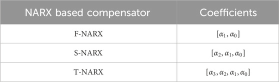
Table 1. Coefficients of the different order NARX model-based compensation.

2.3 Parameter estimation for NARX model-based compensation

In theory, the measured displacement $d_n^m$ should be identical to the command displacement $d_n^c$ when the delay compensation method works perfectly. In this scenario, the relationship between predicted displacements and measured displacements can be expressed as:

$d_n^p=F\left(d_{n-1}^p,\cdots d_{n-i}^p,d_n^m,\cdots d_{n-j}^m\right)(\mathrm{5a})$

or

$d_{n-1}^p=F\left(d_{n-2}^p,\cdots d_{n-i-1}^p,d_{n-1}^m,\cdots d_{n-j-1}^m\right)(\mathrm{5b})$

Given that all $d^p$ and $d^m$ values in Eq. 6b are accessible during RTHS, the NARX model can be derived through data regression between predicted and measured displacements. This model can then be applied to Eq. 2 to compensate time delay. For illustrative purposes, Eq. 4a is employed as an example to illustrate this procedure. By substituting $d_n^c$ with $d_n^m$, Eq. 5a can also be written as

$d_n^p={\displaystyle {\sum }_{k=0}^j}{{\alpha }_{k}d}_{n-k}^m(\mathrm{6a})$

or

$d_{n-1}^p={\displaystyle {\sum }_{k=0}^j}{{\alpha }_{k}d}_{n-k-1}^m(\mathrm{6b})$

However, Eq. 6b comprises only one equation with j+1 undetermined parameters, leading to an under-determined system. Consequently, there exists an infinite number of possible solutions satisfying this equation. To address this challenge and arrive at an appropriate and unique solution, additional constraints must be introduced. In this study, the predicted displacements from previous steps are employed to estimate the undetermined parameters, i.e.,

$d_{n-i}^p={\displaystyle {\sum }_{k=0}^j}{{\alpha }_{k}d}_{n-k-i}^m\left(\mathrm{i}=1,2,\dots M\right)(\mathrm{6c})$

The number of equations, denoted as M, in the parameter estimation process is thereafter referred to as the window length, which is an integer larger than j. It is then obvious from Eq. 6c that the calculated coefficients ${\mathrm{\alpha }}_{\mathrm{k}}$ in NARX-based compensation are not instantaneous undetermined parameters rather parameters estimated through a fixed window length. When the window length is relatively small, the estimated parameters closely approach the current values. Defining ${\mathit{\alpha }}_{\mathit{n}}={\left[{\alpha }_0,{\alpha }_1,\cdots ,{\alpha }_j\right]}^T$, ${\mathit{d}}_{\mathit{n}}^{\mathit{p}}={\left[d_{n-1}^p,d_{n-2}^p,\cdots ,d_{n-L}^p\right]}^{\mathbf{T}}$, ${{\mathit{d}}_{\mathit{n}}^{\mathit{m}}=\left[d_{n-1}^m,d_{n-2}^m,\cdots ,d_{n-L}^m\right]}^{\mathbf{T}}$ and D= $\left[{\mathit{d}}_{\mathit{n}}^{\mathit{m}},{\mathit{d}}_{\mathit{n}-\mathbf{1}}^{\mathit{m}},{\cdots ,\mathit{d}}_{\mathit{n}-\mathit{j}}^{\mathit{m}}\right]$, Eq. 7 can be written as

${\mathit{d}}_{\mathit{n}}^{\mathit{p}}=\mathit{D}{\mathit{\alpha }}_{\mathit{n}}(7)$

In Eq. 7, ${\mathit{d}}_{\mathit{p}}^{\mathit{n}}$ and $\mathit{D}$ can be obtained during RTHS, allowing for the estimation of parameters in NARX model-based compensation through these linear systems of equations. As the window length, denoted as L, is larger than j, Eq. 7 leads to an over-determined system, wherein the number of constraints exceeds the number of unknown variables. Consequently, a solution satisfying the linear system is generally nonexistent. Instead, an approximate solution is sought to minimize a given error. To obtain the estimated parameters, two data regression methods, namely, ordinary least squares and ridge regression, are introduced in this study.

2.3.1 Ordinary least square

The essence of ordinary least squares lies in estimating parameters by minimizing the sum of residual squares, aiming to find ${\widehat{\mathrm{\alpha }}}_{\mathrm{n}}$ appropriate value that satisfies.

${\widehat{\mathrm{\alpha }}}_{\mathit{n}}=\mathit{argmin}{‖\mathit{D}{\mathit{\alpha }}_{\mathit{n}}-{\mathit{d}}_{\mathit{n}}^{\mathit{p}}‖}_{\mathbf{2}}(8)$

where ‘argmin’ represents the argument of the minimum. To identify this minimum, the least-square error is expanded as

${\mathit{\alpha }}_{\mathit{n}}={\left({\mathit{D}}^T\mathit{D}\right)}^{-1}{\mathit{D}}^T{\mathit{d}}_{\mathit{n}}^{\mathit{p}}(9)$

2.3.2 Ridge regression

Ordinary least squares in Eq. 9 offers the best linear unbiased estimation with minimum variance, particularly when the correlation matrix form of D^TD is nearly a unit matrix. However, the practical application of ordinary least squares has limitations, especially when the correlation matrix deviates significantly from a unit matrix. Instead, ridge regression, which is based on estimation from (D^TD+γI), proves to be more suitable (Hoerl and Kennard, 1970) and gives:

${\mathit{\alpha }}_{\mathit{n}}={\left({\mathit{D}}^T\mathit{D}+\gamma \mathit{I}\right)}^{-1}{\mathit{D}}^T{\mathit{d}}_{\mathit{n}}^{\mathit{p}}(10)$

where γ is a real positive number and plays a crucial role in the performance of ridge regression. As the value of γ increases, the total variance decreases, accompanied by an increase in squared bias. Meanwhile, the performance of ridge regression aligns with ordinary least squares when γ is small, but diverges from real values as γ becomes large.

When conducting ridge regression in NARX model-based compensation, it is identical as ordinary least squares when γ equals 0. As γ increases, the calculated ‘a_n’ becomes smaller. In this scenario, the stability of the compensation can be ensured, albeit at the expense of accuracy. To strike a balance between stability and accuracy, ridge regression is primarily applied for compensation methods with three or more parameters, and the range of γ should be carefully selected.

2.4 Discussion of nonlinear terms

Eqs 4a, 4b employ the linear and nonlinear formulation, respectively. The former has exhibited better applicability in real-time hybrid simulation compared to the latter, attributed to the inherent complexity and nonlinearity of hydraulic systems. The linear form can be adapted to various hydraulic systems, while the same cannot be said for the nonlinear form. In this section, the selection of nonlinear terms is very briefly discussed. The nonlinear terms are selected to serve as fine-tuning mechanisms to ensure the stability and accuracy of NARX model-based compensation composed of linear terms. The coefficients of the nonlinear terms are significantly smaller than those of the linear terms, thereby maintaining stability. It should also be noted that identifying suitable nonlinear terms for a specific hydraulic system is a challenging task, even with some preliminary knowledge. Nonetheless, a well-chosen nonlinear system can yield superior compensation performance, capitalizing on the inherent nonlinearity of the hydraulic system.

3 Benchmark model for maRTHS and simulation matrix

3.1 Benchmark model for maRTHS

A novel maRTHS benchmark model has been proposed by Condori Uribe et al. (2023) focusing on a frame subjected to seismic loading at the base. As illustrated in Figure 1, the benchmark model features a steel moment-resisting frame with three bays and three stories. The mid-span at the bottom is designated as the experimental substructure, while the rest is considered as the numerical substructure. To simulate seismic loading, a scaled El Centro historic record serves as the input ground motion, with a scaling factor of 0.40 is applied to maintain linear elastic behavior in all structural components of the frame. For the experimental substructure, two actuators are strategically positioned to deliver equivalent translational and rotational motion. A coupler is employed to facilitate the coupling of the linear stroke of both actuators. A block diagram illustrating the key components, along with a properly designed and tuned control system, is presented in Figure 2A. The objective of this benchmark is to formulate a control system that ensures the output of the controlled plant accurately tracks the target displacement vector. In the benchmark model, an estimator is essential to filter out high-frequency noise before being sent to the control plant. However, this block is typically integrated into the data acquisition module for real RTHS. Consequently, the estimator is not employed for NARX model-based compensation in the benchmark model, as depicted in Figure 2B. Instead, a fifth order Butterworth filter with a cutoff frequency of 6 Hz is utilized in constructing the NARX model to balance the frequency components of the actuator response and noise mitigate performance. The time delay introduced by Butterworth filter is compensated simultaneously, since the displacements after Butterworth filter are sent to the compensator.

Figure 1

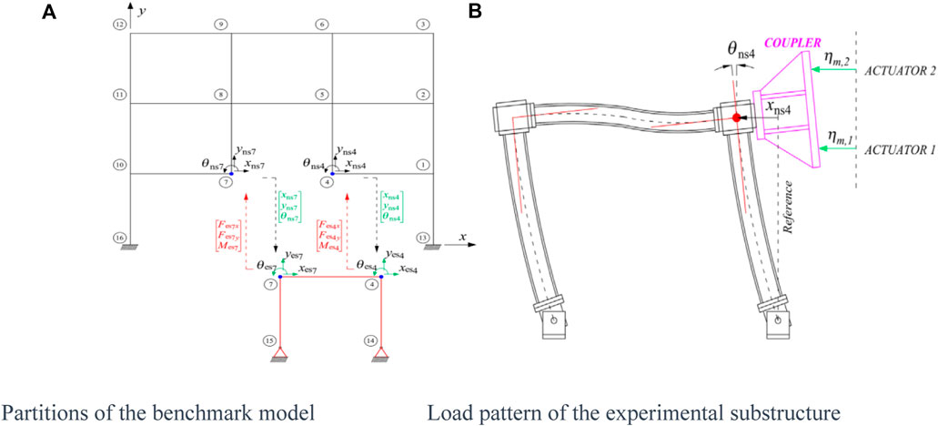
Figure 1. Composition of the benchmark model.

Figure 2

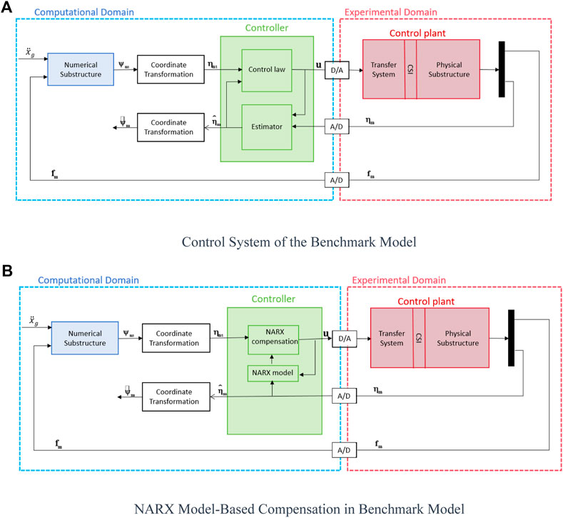
Figure 2. Control system and NARX model-based compensation in the benchmark model.

3.2 Evaluation for maRTHS

To evaluate the performance of NARX model-based compensation for maRTHS, various compensation methods, including traditional inverse compensation (IC), NARX compensation without nonlinear terms (NARX^l), NARX compensation with ridge regression (NARX^r), and NARX compensation with different nonlinear terms (NARXⁿ) are applied to the benchmark model.

3.2.1 Traditional inverse compensation

As the simplest formulation of NARX model-based compensation and a special case of F-NARX, traditional inverse compensation is first implemented, where a₀ and a₁ remain time-invariant during RTHS. Two cases are considered for inverse compensation with different estimated time delays. In Case 1, the estimated time delay is both 25 msec for the first and second actuators, while, the estimated delays are 60 msec. And 25 msec. In Case 2. More details of inverse compensation are presented in Table 2, where a_i,j represents the coefficient a_i for the jth actuator.

Table 2

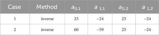
Table 2. Compensation scheme for inverse compensation.

3.2.2 NARX compensation without nonlinear term

When nonlinear terms are not considered, NARX compensation is similar to ATS compensator. In this scenario, various orders with different window lengths are explored. Specifically, Cases 3 to 5 represent second order NARX compensations with window lengths of 512, 1024, and 2048, corresponding to 0.5s, 1.0s, and 2.0s. Additionally, Case 6 to Case 7 maintain a consistent window length of 1024 with different orders, corresponding to firstand fourth order NARX compensation, respectively. Details of NARX compensation without nonlinear terms are summarized in Table 3.

Table 3

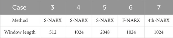
Table 3. Compensation scheme for NARX compensation without nonlinear term.

3.2.3 NARX with rigid regression

Table 4 presents the NARX model-based compensation with rigid regression, where Cases 8 to 11 are presented to compare the performance of the ridge regression using varying regression parameters γ with Case 7 for the fourth order NARX under the window length of 1024. The values of γ for Cases 8 to 11 are 1, 0.01,1 × 10⁻⁷ and 1 × 10⁻⁹, respectively.

Table 4

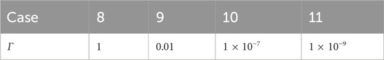
Table 4. Compensation scheme for NARX compensation with ridge regression.

3.2.4 NARX with nonlinear terms

Cases 12 to 16 in Table 5 evaluates the performance of NARX model-based compensation with nonlinear terms, where five different nonlinear terms respectively replace the linear term x_n-2 of S-NARX with a window length of 1024.

Table 5

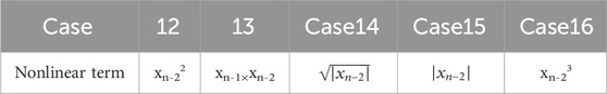
Table 5. Compensation scheme for NARX compensation with nonlinear terms.

3.3 Evaluation criteria

The evaluation of compensation performance involves assessing the difference between measured and calculated displacements. However, tracking performance has limitations in evaluating maRTHS. To comprehensively gauge the effectiveness of various compensation methods, ten distinct evaluation criteria (J₁∼J₁₀) are employed. The initial six criteria focus on evaluating the tracking performance of the control system, while the remaining four concentrate on assessing the global performance of RTHS. Specifically, the ten evaluation criteria are defined as:

$J_{1,i}={\mathit{argmax}}_r\left({\displaystyle \sum _{k=1}^N}{\eta }_{ns,i}\left[k\right]\cdot {\eta }_{m,i}\left[k-r\right]\right)\times 1000/f_s,i=1,2,(\mathrm{11a})$

$J_{2,i}=\sqrt{\frac{{\displaystyle \sum _{k=1}^N}{\left({\eta }_{m,i}\left[k\right]-{\eta }_{ns,i}\left[k\right]\right)}^2}{{\displaystyle \sum _{k=1}^N}{\left({\eta }_{ns,i}\left[k\right]\right)}^2}}\times 100,i=1,2.(\mathrm{11b})$

$J_{3,i}=\frac{\mathit{max}\left(\left|{\eta }_{m,i}\left[k\right]-{\eta }_{ns,i}\left[k\right]\right|\right)}{\mathit{max}\left(\left|{\eta }_{ns,i}\left[k\right]\right|\right)}\times 100,i=1,2.(\mathrm{11c})$

$J_{4,i}={\mathit{argmax}}_r\left({\displaystyle \sum _{k=1}^N}{\eta }_{ns,i}\left[k\right]\cdot {\widehat{\eta }}_{m,i}\left[k-r\right]\right)\times 1000/f_s,i=1,2,(\mathrm{11d})$

$J_{5,i}=\sqrt{\frac{{\displaystyle \sum _{k=1}^N}{\left({\widehat{\psi }}_{m,i}\left[k\right]-{\psi }_{ns,i}\left[k\right]\right)}^2}{{\displaystyle \sum _{k=1}^N}{\left({\psi }_{ns,i}\left[k\right]\right)}^2}}\times 100,i=4,28,(11e)$

$J_{6,i}=\frac{\mathit{max}\left(\left|{\widehat{\psi }}_{m,i}\left[k\right]-{\psi }_{ns,i}\left[k\right]\right|\right)}{\mathit{max}\left(\left|{\psi }_{ns,i}\left[k\right]\right|\right)}\times 100,i=4,28.(\mathrm{11f})$

$J_{7,i}=\sqrt{\frac{{\displaystyle \sum _{k=1}^N}{\left({\widehat{\psi }}_{m,i}\left[k\right]-{\psi }_i\left[k\right]\right)}^2}{{\displaystyle \sum _{k=1}^N}{\left({\psi }_i\left[k\right]\right)}^2}}\times 100,i=4,28,(\mathrm{11g})$

$J_{8,i}=\sqrt{\frac{{\displaystyle \sum _{k=1}^N}{\left({\psi }_{ns,i}\left[k\right]-{\psi }_i\left[k\right]\right)}^2}{{\displaystyle \sum _{k=1}^N}{\left({\psi }_i\left[k\right]\right)}^2}\times 100,}i=2,26,3,27.(\mathrm{11h})$

$J_{9,i}=\frac{\mathit{max}\left(\left|{\widehat{\psi }}_{m,i}\left[k\right]-{\psi }_i\left[k\right]\right|\right)}{\mathit{max}\left(\left|{\psi }_i\left[k\right]\right|\right)}\times 100,i=4,28.(\mathrm{11i})$

$J_{10,i}=\frac{\mathit{max}\left(\left|{\widehat{\psi }}_{ns,i}\left[k\right]-{\psi }_i\left[k\right]\right|\right)}{\mathit{max}\left(\left|{\psi }_i\left[k\right]\right|\right)}\times 100,i=2,26,3,27.(\mathrm{11j})$

where i represents the actuator number in Eqs 11a–11d, and represents the node freedom number in Eqs 11e–11i. In Eqs 11e–11i, ‘4/2/3′ and ‘28/26/27′ represent the x and θ direction responses for the first/second/third floor. ηns, ηm, and ${\widehat{\eta }}_m$ represent the desired actuator displacements, measured actuator displacements, and estimated interface node displacements; ${\widehat{\psi }}_m$, Ψns and Ψ represent the frame target displacements, estimated interface node displacements, and numerical substructure response; f_s represents the sampling frequency and is set at 1024Hz. The ten criteria above can be divided into three categories: J₁ to J₃, J₄ to J₆, J₇ to J₁₀ represent tracking control, estimation results, and global performance, respectively (Uribe et al., 2023). Since the estimator is not adopted in NARX compensation, J₁ is exactly the same as J₄. Consequently, the results of J₄ are not presented in this study.

4 Performance of NARX model-based compensation

The maRTHS benchmark model involves various types of displacements, such as target and measured displacements for each actuator, frame target displacements, and estimated interface node displacements of the experimental frame, as well as reference and estimated measured responses of the frame at the interface node, and reference and numerical substructure responses at each floor. Analyzing time histories of all these displacements offers an accurate and comprehensive way to assess the compensation’s performance. However, in many cases, different displacements are correlated. As such, the performance of the compensation can be effectively reflected in the difference between the reference and estimated measured response of the frame at the interface node. Consequently, only the time history of the reference and estimated measured responses of the frame at the first floor is provided. In order to accurately obtain the patterns of compensation methods under various working conditions, no upper and lower limits of the coefficients are used for any case. The tracking control and estimation results are firstly analyzed to obtain the performance of different compensation performance.

4.1 Performance of traditional inverse compensation

The performance of traditional inverse compensation can be assessed through Case 1 and 2, with the reference and the measured displacements of the first floor depicted in Figure 3 for both cases. It is evident that the measured displacement for Case 2 is closer to the reference, indicating that Case 2 outperforms Case 1. The evaluation criteria are presented in Table 6 for inverse compensation. It can be observed that all criteria for Case 2 are superior to those for Case 1, which is consistent with observations in Figure 3. Given that a₀ and a₁ remain time-invariant throughout the simulation, the performance of inverse compensation is highly dependent on the initial estimation. From J_1,1 and J_1,2 for Case 2, inverse compensation proves effective in reducing time delay when the initial estimation is accurate. However, a notable time delay is observed when the initial estimation deviates from actuator dynamics, as observed in J_1,1 for Case 1.

Figure 3

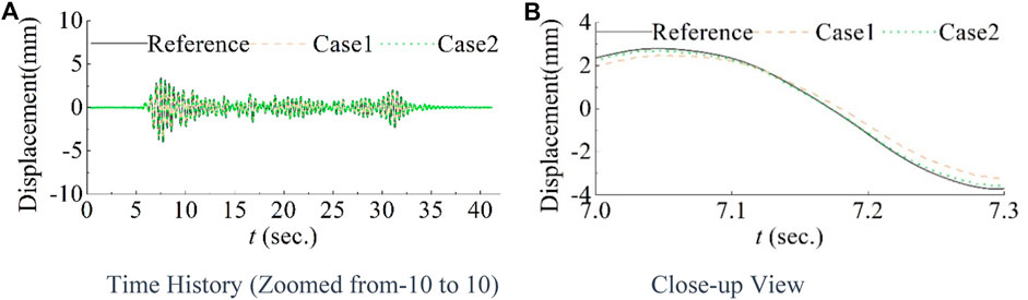
Figure 3. Comparison of measured first floor displacements for inverse compensation.

Table 6

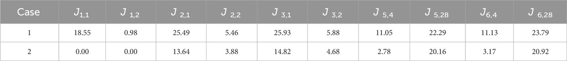
Table 6. Evaluation Criteria for Inverse Compensation with tracking control and estimation results.

An intriguing observation arises when comparing the tracking criteria of the second actuator, namely, J_1,2, J_2,2, and J_3,2, for the two cases. Despite employing the same initial estimations for both cases, the tracking criteria for Case 2 surpass those for Case 1. This can be attributed to the interaction between the two actuators in maRTHS. Consequently, full compensation of dynamics is imperative all actuators in maRTHS. This might stem from inadequate compensation altering the properties of the structural response, particularly the frequency components. Hence, compensation parameters that were initially suitable may become unsuitable. However, this issue is primarily associated with constant delay compensation methods, and it can be effectively addressed through adaptive compensation.

When comparing tracking criteria of the same actuator, namely, J₁, J₂, and J₃ for the same case, the performance of the second actuator is significantly better. In Case 1, the substantial difference between the two actuators is attributed to the initial estimation. However, both J₁ values are zero for both actuators in Case 2, while J₂ and J₃ are nearly three times higher for the first actuator compared to the second actuator. This discrepancy suggests that, in comparison with the second actuator, the actuator delay for the first actuator is more pronounced. In such cases, traditional constant delay compensation is unsuitable, and adaptive compensation becomes necessary. Moreover, the estimated results for x direction responses, i.e., J_5,4 and J_6,4, is reduced from about 11% for case 2%–3% for case 1. This implies the importance of initial estimation for inverse compensation. However, the estimated results for θ direction responses, i.e., J_5,28 and J_6,28, have little improvement. This however indicates the requirement of adaptive compensation.

4.2 Influence of the window length and order for NARX model-based compensation

The window length and the model order are two major factors that influence the performance of NARX model-based compensation. Cases 3 to 5 are employed to demonstrate the impact of window length on the performance of second order NARX model-based compensation without nonlinear terms. Figure 4 presents the comparison of measured first-floor displacements for these three cases. It can be observed in Figure 4A that it is evident that the measured displacement in cases 4 and 5 aligns quite well with the reference. In Case 3, the fluctuations in displacement over the last 15 s indicate instability. Additionally, in Figure 4B, none of the measured displacements exactly match the reference, suggesting that the delay compensation method can reduce but cannot eliminate time delay, even for NARX model-based compensation.

Figure 4

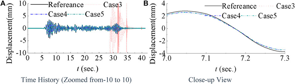
Figure 4. Comparison of measured first-floor displacements for NARX model-based compensation with different window length.

The evaluation criteria for NARX model-based compensation with different window lengths when considering tracking control and estimation results are presented in Table 7. Criteria are small and nearly identical for Case 4 and 5, while larger values criteria are observed for Case 3. Constructing the NARX model requires a certain amount of data, otherwise the NARX model may deviate from actuator dynamics. Thus, there is a limit on the minimum data length for NARX model-based compensation. When the window length is smaller than the limit, the performance of compensation deteriorates, as observed for Case 3. Once the minimum data length is reached, increasing the window length has little impact on performance, as observed from the minimal difference between Case 4 and 5. Although computational efficiency and response to time-varying delays might decrease with an increase of window length. When comparing Case 4 and 2, the NARX model-based compensation outperforms inverse compensation in all tracking evaluation criteria, i.e., J₁ to J₃, especially for J_2,1. Consequently the estimated results for θ, i.e., J_5,28 and J_6,28, direction responses is reduced from about 20% to 2% when NARX model-based compensation utilized.

Table 7

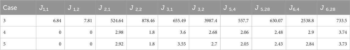
Table 7. Evaluation criteria for NARX model-based compensation with different window length.

The performance of NARX model-based compensation is determined by the parameters of the NARX model. Since the same compensation method is applied for both actuators, the parameters of the NARX model are nearly identical for Case 4 and 5. Therefore Figure 5 only presents the compensation parameters for the first actuator for Case 3 and 4. When nonlinear terms are not considered, the sum of a should be close to 1. From Figure 5, a₀ and a₂ are similar, while a₁ is almost the opposite of the sum of a₀ and a₂ for both cases. In Figure 5A, the parameters undergo dramatic changes from 11 s to 15 s, 20 s to 25 s, and 28 s to the end of the simulation. Large value of a₁ is observed more than 10,000 around 28 s, which corresponds to the time when measured displacement deviates from the reference and the simulation becomes unstable. On the contrary, the parameters in Figure 5B do not have a significant change, resulting in better compensation performance. This again indicates the importance of window length in NARX model-based compensation.

Figure 5

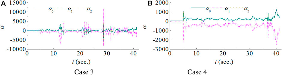
Figure 5. Parameters of NARX model for the first actuator.

Case 4, 6, and seven all have window length of 1024 and are used to assess the impact of model order on NARX model-based compensation without nonlinear terms. Figure 7 displays the time history of the first-floor measured displacements for these cases compared with the reference. Instability is observed in Case 7 when a fourth order NARX model is employed, whereas Case 6, using a first order NARX model, closely resembles case 4 with a second order NARX model. Table 8 presents the criteria for Case 6 and 7, which is consistent with observations from Figure 6. This suggests that while higher order NARX models may become unstable for the same window length, stability can be maintained with lower order NARX models. Additionally, lower order models require fewer parameters, allowing for accurate parameter estimation with smaller window lengths. The compensation parameters are presented in Figure 7 for Case 6 and 7. In Figure 7A, a₀ remains approximately 50 for the first order NARX compensation, except around 7 s and in the last 2 s. Furthermore, the sum of a₀ and a₁ is close to 1. In contrast, the parameters for the fourth order NARX model can reach up to 8×10⁷, resulting in significantly larger evaluation criteria in Table 8 for Case 7.

Table 8

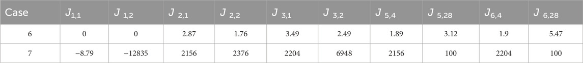
Table 8. Evaluation criteria for NARX model-based compensation with different orders.

Figure 6

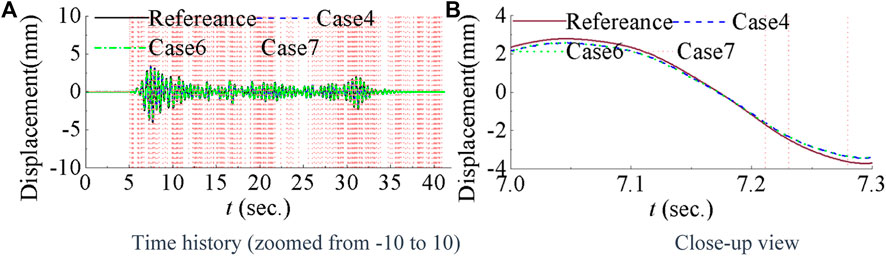
Figure 6. Illustrates a comparison of measured first-floor displacements for NARX model-based compensation with varying orders.

Figure 7

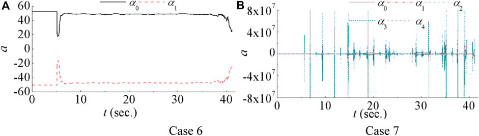
Figure 7. Illustrates the parameters of the NARX model for the first actuator.

4.3 Influence of rigid regression

Due to smaller window length than the minimum for the fourth order NARX model, From Figure 6 and Table 8, it is evident that the measured displacement for Case 7 becomes unstable. This results in inability for high order NARX model-based compensation. It is apparent that traditional ordinary least square has limitations, especially when the number of undetermined parameters is more than three in the NARX model. Rigid regression, instead of ordinary least square, is employed in Case 8–11 to calculate parameters in the fourth order NARX model with different values of parameter γ. The time histories of compensation parameters are presented in Figure 8 and the corresponding values of evaluation criteria are summarized in Table 9.

Figure 8

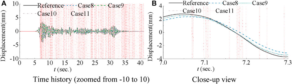
Figure 8. Comparison of measured first floor displacements for NARX model based with rigid regression.

Table 9

Table 9. Evaluation criteria for NARX model-based compensation with rigid regression.

In Figure 8A, it can be observed that Case 11 remains unstable due to γ value as small as 1 × 10⁻⁹, indicating that the rigid regression does not take effect. For very small value of γ, rigid regression is same as ordinary least square regression. With the increase of γ, cases 8–10 become stable such as case 10 when γ equals 1 × 10⁻⁷. Compared with case 4 in Table 7, the evaluation criteria in Table 9 for case 10 are better for almost all criteria. This suggests the advantages of the higher order NARX model-based compensation with ridge regression. When γ increases to 0.01, the tracking error visibly increases for the first actuator, while a slight increase is observed for the second actuator as shown in Table 9. Moreover, a significant increase can be observed for all evaluation criteria when γ increases to 1. Consequently, ridge regression would reduce the performance of compensation when γ reaches a threshold. However, the simulations remain stable for larger γ. The parameters for Case 11 are like those of Case 7, while Case 9 falls between Case 8 and 10. Thus, only the parameters of the NARX model for the first actuator for Case 8 and Case 10 are presented in Figure 9. It can be observed that the absolute value of each compensation parameter decreases with the increase of γ. Influence of nonlinear term.

Figure 9

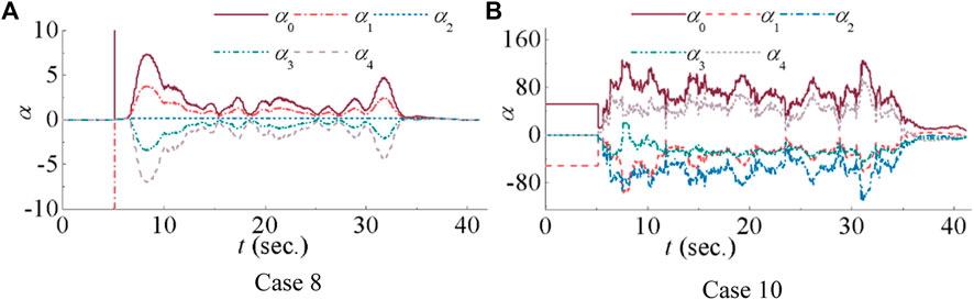
Figure 9. Parameters of the NARX model for the first actuator with rigid regression.

Nonlinear terms are explored in this study for the NARX model-based compensation. In Figure 10A, clear instability is observed for Case 15, while the rest cases remain stable. In the close-up view of Figures 10A, B slight difference between the measured displacement and reference is observed for Case 16, while the measured displacements in the remaining cases agree well with the reference. This implies that different nonlinear term leads to distinct compensation performance. The evaluation criteria are summarized in Table 10 for the five cases with nonlinear terms. It is worth noting that Case 12 and 13, which involve x_n-2² with little difference from x_n-1×x_n-2, have almost identical evaluation criteria. In comparison with corresponding case 4 with only linear terms, these criteria are slightly larger. Conversely, Case 14 demonstrates improved evaluation criteria particularly with smaller tracking control when compared with corresponding linear case. This observation suggests that the inclusion of a carefully selected nonlinear term can further improve the performance of the NARX model-based compensation. However, large evaluation criteria are noticeable for Case 15 and 16, consistent with observations in Figure 10.

Figure 10

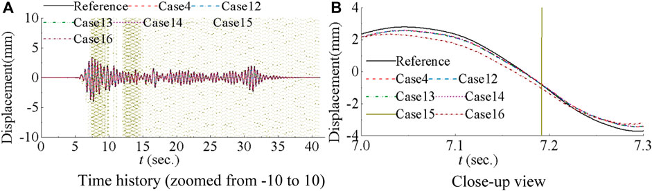
Figure 10. Comparison of measured first-floor displacements for NARX model-based compensation with different nonlinear terms.

Table 10

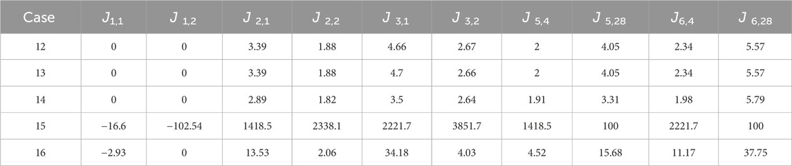
Table 10. Evaluation criteria for NARX model-based compensation with various nonlinear terms.

In the context of utilizing a second order NARX model for compensation, three key parameters (a₀, a₁, a₂) are derived during the simulation. While the behavior of a₀ and a₁ aligns with the first order NARX model compensation as shown in Figure 7A, the focus in Figure 11 is exclusively on the time history of the third parameter a₂. From Figure 11A, it can be observed that a₂ exhibits slight variation ranging between −0.015 and 0.01. This magnitude is notably smaller when compared to a₀ and a₁ from Figure 7A. This observation underscores the nuanced and fine-tuning role played by the nonlinear term in shaping the compensation performance. In particular, the trajectories of a₂ for cases 12, 13, and 16 remain relatively small throughout the simulation with occasional jumps. Conversely, for case 15, the absolute values of a₂ surpass 200, indicative of significant fluctuations, ultimately contributing to worse compensation performance.

Figure 11

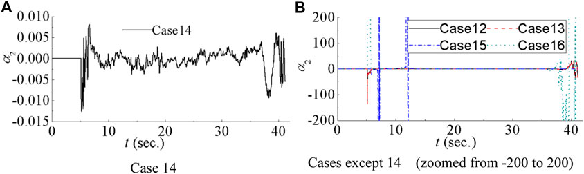
Figure 11. Parameters of NARX model for the first actuator with nonlinear terms.

4.4 Global performance of NARX model-based compensation

As maRTHS incorporates a minimum of two actuators, a comprehensive global evaluation becomes imperative. Given that cases 3, 7, 8, 11, and 15 have been established as unstable through simulation, the remaining 11 cases are used to evaluate the performance of NARX model-based compensation. Figure 12 presents the global performance evaluation criteria (J₇ to J₁₀) for these cases.

Figure 12

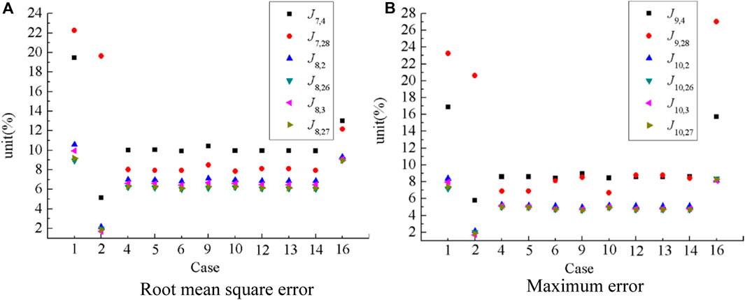
Figure 12. Global performance of NARX model-based compensation.

It can be observed that case 2 exhibits the best global performance among all stable cases, while case 1 shows the worst global performance evaluation criteria, with the exception of the θ direction responses for the first floor. This observation confirms previous finding that the performance of constant delay compensation significantly rely on initial estimation. Notably, the values for the second and third floors (J₈ and J₁₀) in case 2 are surprisingly lower than those in NARX-model-based compensation. This might be attributed to the reduction in testing errors for the x and θ directions when calculating the response of the second and third floors. Consequently, it becomes apparent that improving the tracking performance of individual actuators does not necessarily translate to an enhancement in the global performance of maRTHS, which is distinct from saRTHS. Figure 13.

Figure 13

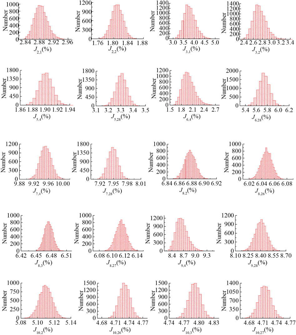
Figure 13. Distribution of evaluation criteria for case 14.

5 Robustness of NARX model-based compensation

The analysis in previous section has demonstrated the effectiveness of the NARX model-based compensation method in maRTHS. In addition to accounting for measured responses, this method also considers noise, uncertainties, or model inaccuracies in the control plant as part of the benchmark model, enabling robustness analysis. Although rigid regression enhances the robustness of higher order NARX model-based compensation method, it is crucial to note that the performance of rigid regression is contingent upon the regression parameter γ, which, though significant, will not be delved into in this discussion.

To evaluate the impact of system uncertainties, an initial set of 10,000 simulations is conducted for the no-compensation case. Subsequently, an additional 10,000 simulations with different control plant uncertainties are carried out for Case 4 and 14, shedding light on the robustness of the NARX model-based compensation with both linear and nonlinear terms. Tables 11–13 present the mean and standard deviation (std) of evaluation criteria for the no-compensation scenario, Case 4, and Case 14. Specifically, Table 11 summarizes the statistics for the no-compensation case, where the std ranges from 0.19 to 1.11 across different criteria, representing 0.9%–8.8% of corresponding mean values.

Table 11

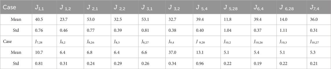
Table 11. The mean and stand derivation (std) of no compensation case.

Table 12

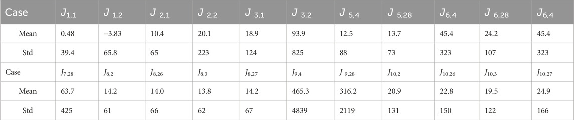
Table 12. The mean and stand derivation (std) of case 4.

Table 13

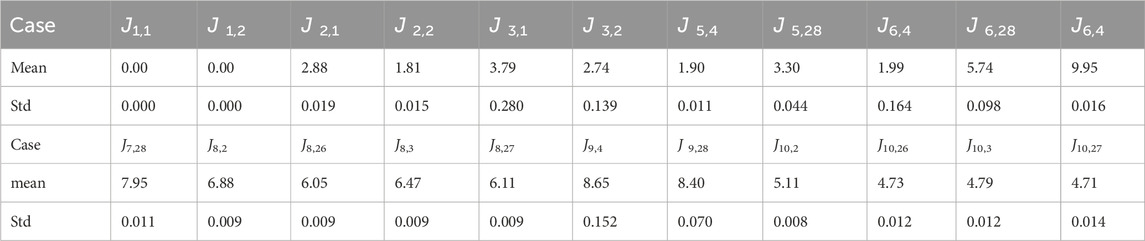
Table 13. The mean and stand derivation (std) of case 14.

In contrast, Table 12 shows a significant std variation from 61 to 4839 for Case 4, indicating instability for the second order NARX model-based compensation in the absence of nonlinear terms. The average delay for both actuators are no longer 0, especially for the second actuator. This implies again the importance of including nonlinear terms or rigid regression for stability. Considering the incorporation of nonlinear terms in NARX model-based compensation, Table 13 enumerates the 22 assessment criteria for Case 14. Average delay for both actuators are 0 with 0 standard deviation, which indicates no instability occurs. The standard deviation ranges from 0 to 0.28 across various criteria, constituting 0.1%–8.2% of their respective mean values. Compared with no compensation cases in Table 11, the introduction of nonlinear term not only improves the accuracy but also increase the robustness of the simulation. This underscores the commendable performance of the NARX model-based compensation when nonlinear terms are taken into account.

6 Summary and conclusion

This study presents the performance evaluation of NARX model-based compensation for multi-axial real-time hybrid simulation (maRTHS) benchmark model. Traditional inverse compensation is also considered as the simplest formulation of NARX model compensation. Different window length and NARX model order are accounted for searching for patterns of NARX model-based compensation through linear terms. Rigid regression technique is utilized to estimate the model coefficients for higher order NARX model-based compensation. Different nonlinear terms are selected to prove the effectiveness of the nonlinear model. A total of 10,000 perturbed simulations are conducted to verify the robustness of NARX model-based compensation. Based on the results of this study, conclusions are drawn as follows:

1. As a special case of NARX model-based compensation, inverse compensation utilizes a fixed first order ARX model during simulation, which the tracking performance highly depends on the initial estimation. Moreover, perfect compensation performance cannot be reached even the initial estimation consistent with actuator dynamics. However, inverse compensation may provide good globe global evaluation for maRTHS. Moreover, the compensation performance of one actuator may influence the performance of other actuators for maRTHS, which is different from traditional single actuator RTHS.

2. The suitable window length for NARX model-based compensation depends on the order of NARX model. Higher order model has larger number of uncertain parameters thus requiring longer window length. There is a length threshold for a certain order NARX model-based compensation. The compensation effect becomes very poor when the window length is smaller than threshold, but will not significantly improves when window length larger than this threshold.

3. Compared with ordinary least square, ridged regression sacrifices part of accuracy to improve stability, which is particularly suitable for higher order NARX model-based compensation. Ridged regression decreases the length threshold, thus the advantages of the high order NARX model can be demonstrated. The performance of ridged regression is highly depending on parameter λ. A small λ leads ridged regression degenerating to ordinary least square, while large λ damage the accuracy of compensation completely.

4. Identifying an appropriate nonlinear term poses a challenge in NARX model-based compensation. However, the judicious selection of a suitable nonlinear term can significantly enhance both accuracy and robustness in compensation performance. Typically, a harmonious blend of linear and nonlinear terms is employed to strike a balance between accuracy and stability. In such instances, nonlinear terms contribute to refining the overall compensation effect. The outcomes of 10,000 perturbed simulations highlight that well-chosen nonlinear terms can indeed bolster the robustness of NARX model-based compensation with high accuracy.

5. Actuator control for maRTHS presents greater challenges compared to saRTHS. Improving the tracking performance of individual actuators may not necessarily result in an overall enhancement of maRTHS performance. Therefore, the adoption of advanced compensation techniques with higher accuracy and robustness is necessary for effective control of maRTHS

Data availability statement

The raw data supporting the conclusion of this article will be made available by the authors, without undue reservation.

Author contributions

WX: Data curation, Funding acquisition, Investigation, Resources, Software, Validation, Visualization, Writing–original draft, Writing–review and editing. XM: Data curation, Software, Visualization, Writing–original draft. CC: Conceptualization, Methodology, Supervision, Writing–review and editing. TG: Methodology, Project administration, Resources, Supervision, Writing–review and editing. CP: Data curation, Validation, Visualization, Writing–original draft.

Funding

The author(s) declare that financial support was received for the research, authorship, and/or publication of this article. The first author would like to acknowledge the support from the Ministry of Science and Technology of China under grant No. 2023YFC3804300 and National Science Foundation of China under grant No. 52178114, Young scientific and technological talents promotion project of Jiangsu Association for science and technology No. 2021-79.

Conflict of interest

The authors declare that the research was conducted in the absence of any commercial or financial relationships that could be construed as a potential conflict of interest.

Publisher’s note

All claims expressed in this article are solely those of the authors and do not necessarily represent those of their affiliated organizations, or those of the publisher, the editors and the reviewers. Any product that may be evaluated in this article, or claim that may be made by its manufacturer, is not guaranteed or endorsed by the publisher.

References

Carrion, J. E., and Spencer, B. F. (2008). Real-time hybrid testing using model-based delay compensation. Smart Struct. Syst 4, 809–828. doi:10.12989/sss.2008.4.6.809

CrossRef Full Text | Google Scholar

Chae, Y., Kazemibidokhti, K., and Ricles, J. M. (2013). Adaptive time series compensator for delay compensation of servo-hydraulic actuator systems for real-time hybrid simulation. Earthq. Eng. Struct. Dyn. 42, 1697–1715. doi:10.1002/eqe.2294

CrossRef Full Text | Google Scholar

Chen, C., and Ricles, J. M. (2008). Stability analysis of SDOF real-time hybrid testing systems with explicit integration algorithms and actuator delay. Earthq. Eng. Struct. Dyn. 37, 597–613. doi:10.1002/eqe.775

CrossRef Full Text | Google Scholar

Chen, C., and Ricles, J. M. (2012). Large-scale real-time hybrid simulation involving multiple experimental substructures and adaptive actuator delay compensation. Earthq. Eng. Struct. Dyn. 41, 549–569. doi:10.1002/eqe.1144

CrossRef Full Text | Google Scholar

Hoerl, A. E., and Kennard, R. W. (1970). Ridge regression - biased estimation for nonorthogonal problems. Technometrics 12, 55–67. doi:10.1080/00401706.1970.10488634

CrossRef Full Text | Google Scholar

Horiuchi, T., Inoue, M., Konno, T., and Namita, Y. (1999). Real-time hybrid experimental system with actuator delay compensation and its application to a piping system with energy absorber. Earthq. Eng. Struct. Dyn. 28, 1121–1141. doi:10.1002/(sici)1096-9845(199910)28:10<1121::Aid-eqe858>3.3.Co;2-f

CrossRef Full Text | Google Scholar

Leontaritis, I. J., and Billings, S. A. (1985). Input-output parametric models for non-linear systems Part I: deterministic non-linear systems. Int. J. Control 41, 303–328. doi:10.1080/0020718508961129

CrossRef Full Text | Google Scholar

Li, N., Tang, J. C., Li, Z. X., and Gao, X. Y. (2022). Reinforcement learning control method for real-time hybrid simulation based on deep deterministic policy gradient algorithm. Struct. Control Health Monit. 29, e3035. doi:10.1002/stc.3035

CrossRef Full Text | Google Scholar

Lu, L. Q., Wang, J. T., Ding, H., and Zhu, F. (2022). Theoretical and experimental studies on critical time delay of multi-DOF real-time hybrid simulation. Earthq. Eng. Eng. Vib. 21, 117–134. doi:10.1007/s11803-021-2073-0

CrossRef Full Text | Google Scholar

Najafi, A., Fermandois, G. A., Dyke, S. J., and Spencer, B. F. (2023). Hybrid simulation with multiple actuators: a state-of-the-art review. Eng. Struct. 276, 115284. doi:10.1016/j.engstruct.2022.115284

CrossRef Full Text | Google Scholar

Nakashima, M., Kato, H., and Takaoka, E. (1992). Development of real-time pseudo dynamic testing. Earthq. Eng. Struct. Dyn. 21, 79–92. doi:10.1002/eqe.4290210106

CrossRef Full Text | Google Scholar

Ning, X. Z., Wang, Z., Zhou, H. M., Wu, B., Ding, Y., and Xu, B. (2019). Robust actuator dynamics compensation method for real-time hybrid simulation. Mech. Syst. Signal Process 131, 49–70. doi:10.1016/j.ymssp.2019.05.038

CrossRef Full Text | Google Scholar

Ou, G., Ozdagli, A. I., Dyke, S. J., and Wu, B. (2015). Robust integrated actuator control: experimental verification and real-time hybrid-simulation implementation. Earthq. Eng. Struct. Dyn. 44, 441–460. doi:10.1002/eqe.2479

CrossRef Full Text | Google Scholar

Palacio-Betancur, A., and Soto, M. G. (2023). Recent advances in computational methodologies for real-time hybrid simulation of engineering structures. Arch. Comput.Methods Eng. 30, 1637–1662. doi:10.1007/s11831-022-09848-y

CrossRef Full Text | Google Scholar

Silva, C. E., Gomez, D., Maghareh, A., Dyke, S. J., and Spencer, B. F. (2020). Benchmark control problem for real-time hybrid simulation. Mech. Syst. Signal Process 135, 106381. doi:10.1016/j.ymssp.2019.106381

CrossRef Full Text | Google Scholar

Tian, Y. P., Shao, X. Y., Zhou, H. M., and Wang, T. (2020). Advances in real-time hybrid testing technology for shaking table substructure testing. Front. Built Environ. 6, 123. doi:10.3389/fbuil.2020.00123

CrossRef Full Text | Google Scholar

Uribe, J. W. C., Salmeron, M., Patino, E., Montoya, H., Dyke, S. J., Silva, C. E., et al. (2023). Experimental benchmark control problem for multi-axial real-time hybrid simulation. Front. Built Environ. 9, 1270996. doi:10.3389/fbuil.2023.1270996

CrossRef Full Text | Google Scholar

Wallace, M., Sieber, J., Neild, S., Wagg, D., Krauskopf, B., and Asme, A. (2005). “Delay differential equation models for real-time dynamic substructuring,” in 5th International Conference on Multibody Systems, Nonlinear Dynamics, and Control, Long Beach, CA, Sep 24-28 2005 (ASME), 875–882.

CrossRef Full Text | Google Scholar

Wang, Z., Ning, X. Z., Xu, G. S., Zhou, H. M., and Wu, B. (2019). High performance compensation using an adaptive strategy for real-time hybrid simulation. Mech. Syst. Signal Process 133, 106262. doi:10.1016/j.ymssp.2019.106262

CrossRef Full Text | Google Scholar

Xu, W., Tong, G., and Cheng, C. (2016). Comparison of delay compensation methods for real-time hybrid simulation using frequency-domain evaluation index. Earthq. Eng. Eng. Vib. 15, 129–143. doi:10.1007/s11803-016-0310-8

CrossRef Full Text | Google Scholar

Xu, W. J., Chen, C., Gao, X. S., Chen, M. H., Guo, T., and Peng, C. L. (2022). Data-driven nonlinear autoregressive with external input model-based compensation for real-time testing. Struct. Control Health Monit. 29, e3119. doi:10.1002/stc.3119

CrossRef Full Text | Google Scholar

Xu, W. J., Chen, C., Guo, T., and Chen, M. H. (2019). Evaluation of frequency evaluation index based compensation for benchmark study in real-time hybrid simulation. Mech. Syst. Signal Process 130, 649–663. doi:10.1016/j.ymssp.2019.05.039

CrossRef Full Text | Google Scholar

Zhou, H. M., Xu, D., Shao, X. Y., Ning, X. Z., and Wang, T. (2019). A robust linear-quadratic-Gaussian controller for the real-time hybrid simulation on a benchmark problem. Mech. Syst. Signal Process 133, 106260. doi:10.1016/j.ymssp.2019.106260

CrossRef Full Text | Google Scholar