Transient Diffusion in Bi-Layer Composites With Mass Transfer Resistance: Exact Solution and Time Lag Analysis

1. Introduction

The mathematical description of the transient behavior of a composite membrane and, in particular, bi-layer composite membranes, has important implications in drug release devices from planar matrix devices (Cabrera et al., 2006; Cabrera and Grau, 2007), in drug delivery through the skin (Ghanem et al., 1987; Couto et al., 2014), in the study of the cornea (Cooper and Kasting, 1987; Couto et al., 2014), studying the role of membranes in keeping compounds from contaminating the surroundings (Kalbe et al., 2002; Edil, 2003), in vacuum insulation panels that creates high performance thermal insulation (Garnier et al., 2011), mass diffusion of neutral species in the fabrication of multi-layer thin-film (Goldner et al., 1992), metallic thermal protection system (Gu et al., 2016), semiconductor composite in bi-layer organic solar cells (Hatton et al., 2007), biodegradable bi-layer film barrier using gelatin and chitosan (Rivero et al., 2009), gas transport in inorganic/organic hybrid structures (Jang and Han, 2009), and gas barrier of organic-inorganic hybrid coatings (Minelli et al., 2010), When modeling the phenomena of heat conduction or gas permeation, the exchange of heat or chemical at the surfaces contacting with the medium are often assumed to occur “infinitely” fast. Mathematically, this translates into the assumption that the temperature (for heat conduction) or concentration (for mass transfer) of the bi-layer at the surface equates that of the contacting medium, simplifying greatly the calculations necessary to find an analytical solution. The contacting medium is generally considered to be maintained at a constant temperature or concentration. To account for boundary effects as shown in Figure 1A, whether this means heat convection, diffusion-limited reaction at the surface or mass transfer resistance, the constant boundary condition can be altered to:

$\frac{dC}{dt}=B\left(C-C_{\infty }\right)(1)$

with $C_{\infty }$ being the concentration of the solution and assuming that the volume of the contacting solution is of large enough volume that its concentration is invariant. For example, in fuel resistance of rubber where phenomena of absorption of the fluid on the exposed side of the rubber membrane and desorption on the other side play important roles the transient behavior of this membrane (Forte and Leblanc, 1992). Frisch showed the benefits of a boundary-layer resistance in the form of a protective film layer on top of polymer membranes (Frisch et al., 1984). Boundary effects are seen in food packaging with polymer films to reduce the permeation of oxygen or water (Smith and Peppa, 1991; Laoubi and Vergnaud, 1996). A film barrier can also form during dispersed-drug release from planar matrices (Zhou and Wu, 2002) that, without adequate accounting of these boundary effects, leads to an underestimation of the drug amount released into the medium. Another important implication of boundary layers appear in the context of rotating disc electrodes (Levich, 1962; Gough and Leypoldt, 1980).

FIGURE 1

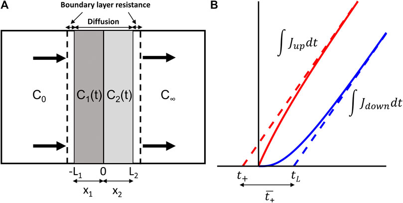
FIGURE 1. (A) Schematic of a bi-layer composite with mass transfer resistance and (B) representative examples of the mass permeated or, equivalently, the integrals of the upstream and downstream fluxes J (shown in red and blue, respectively).

There have been considerable efforts in developing solutions to bi-layer systems involving the mass-transfer limited boundary conditions (Equation 1). Ramkrishna and Amundson (Ramkrishna and Amundson, 1974), as well as (Mikhailov et al., 1983), have proposed solution schemes based on solving the eigenvalues and eigenfunctions of a Sturm-Louiville type system to study the transient heat conduction behavior of composites undergoing convection type boundary conditions. Antonopoulos and Tzivanidis (Antonopoulos and Tzivanidis, 1996) outlined a procedure to evaluate transient heat conduction in n-layer composites with a convection type of boundary condition combining the separation of variables technique with an orthogonal expansion of the functions. Yet, the analytical, as opposed to numerical, evaluation of the eigenvalues, eigenfunctions, and the integral relationships arising from these approaches generally remains challenging for a bi-layer composite undergoing convective effects. This technique was further developed to investigate the approximate behavior of heat conduction with combined radiative and convective boundary conditions (Miller and Weaver, 2003) through a linearization of the radiative effects. An ‘analytical’ method of this problem was also developed by de Monte (de Monte, 2000; de Monte, 2002) based on Vodicka’s approach and applied to one-dimensional media to study unsteady heat conduction and extending to n-layers. We also note related works by Goldner et al. (1992) who obtained the analytical equations to a bi-layer diffusion system subjected to an impenetrable wall boundary using the Inversion theorem of Laplace transforms. Subramanian and White (Subramanian and White, 2001) derived an exact solution to a bi-layer composite undergoing galvanostatic boundary conditions using a modified separation of variables method.

In addition to the importance of modeling the transient response in a permeation process, especially for slowly diffusing processes, the “integral permeation” method has played a key role in the determination of the physical properties of a membrane, and in particular, its constitutive diffusion coefficients and permeability constants (Rutherford and Do, 1997). By dividing the permeation process into its transient and steady-state components as shown in Figure 1B, one can represent the transient component by a “time lag” parameter. This concept was introduced in the work of Daynes (1920) and Barrer and Rideal (1939). These findings outlined the now widely used relationship of the time lag (t_lag) for a single layer with assumptions of constant concentrations maintained on either side of a single-layer material:

$t_{lag}=\frac{L^2}{6D}(2)$

with L being the thickness and D being the diffusion coefficient of the material. Also in Figure 1B, the steady-state components of the upstream and downstream mass permeated are extended using the dashed lines and their x-axis intercepts represent the lead time t₊ and the time lag t_L. The forward mean first passage time is provided by $\overline{t_{+}}=t_L-t_{+}$. The time lag technique has since been expanded to permeation with non Fickian diffusion, polymer membranes, reaction, metallic solids, through catalyst particles among other things (Rutherford and Do, 1997). Notably, there has been an extended amount of work on the characterization of composite membranes using the time lag approach (Jaeger, 1950; Frisch, 1957, 1958; Frisch, 1959; Pollack and Frisch, 1959; Ash et al., 1963, 1965; Siegel, 1991; Liang and Siegel, 2006; Al-Qasas et al., 2014).

In this work, the closed-form and exact transient solutions to a single-layer material and a bi-layer composite undergoing mass transfer resistance at its outside boundaries are derived using the Laplace Inversion Theorem (Jaeger, 1950). The time lag and steady-state components of the transient response to an input step function are also derived. This work aims to support the characterization of bi-layer composites that have significant boundary layer effects. The presented solutions are also shown to be a generalization to various existing solutions in the literature. In addition to the similarities between diffusion and heat conduction, we also show how the solution forms presented in this work can be used to study the transient responses of bi-layer composites to inputs more complex than the usual step function.

2. Theoretical Analysis

A schematic of the problem is shown in Figure 1A. For both the single-layer and bi-layer derivation, the flow within the composite is assumed to follow Fick’s second law with mass transfer resistance occurring at the external boundaries. The assumed direction of the flow is from left to right.

2.1. Diffusion in a Single-Layer with Transfer Resistance

Let us note that the following derivation of the single-layer is equivalent to that of Ash (2001). The key differences with that work are the use of different constant definitions and the application of the nondimensionalization of the parameters. This subsection was written in an effort to provide results that are consistent between the previously derived single-layer and the newly derived bi-layer solutions as well as making comparisons with other results in the literature under one set of notations.

2.1.1. Single-Layer Diffusion with Upstream and Downstream Transfer Resistance

The phenomenon of diffusion is modeled using “Fick’s 2^nd Law,” i.e., Crank (1979):

$\frac{\partial C}{\partial t}=D\frac{{\partial }^{2}C}{\partial x^2}(3)$

subject to the boundary and initial conditions:

$C\left(x,0\right)=\mathrm{0,0}\le x\le L,(4)$

$\frac{\partial C}{\partial x}\left(0,t\right)=B_1\left(C\left(0,t\right)-C_0\right),(5)$

and

$\frac{\partial C}{\partial x}\left(L,t\right)=-B_{2}C\left(L,t\right).(6)$

$\left[B_1=\frac{k_1}{D_1},B_2=\frac{k_2}{D_2}\right](7)$

The convention C(x,t) is used throughout the paper. B₁ and B₂ are the Biot numbers for systems with heat conduction undergoing heat convection at the outside boundaries, the mass transfer Biot numbers in mass diffusion processes or the reaction constant for a first-order reaction. The Biot number is a quantity that relates the inner diffusion to the mass transfer resistance at the surface. Let’s note that when both B₁ and $B_2\to \mathrm{\infty }$, these conditions reduce the problem to that with the analytical solution derived by Daynes (1920).

Dimensionless variables for the concentration, time, and position are introduced:

$c=\frac{C}{C_0},\tau =\frac{Dt}{L^2},y=\frac{x}{L}.(8)$

The dimensionless quantity τ is also known as the mass Fourier number, which can be thought as the ratio between the diffusive transport rate and the storage rate. By using the introduced dimensionless variables and transforming Equation 3 into the Laplace domain, the relation with time is transformed into a dependence on the complex variable s:

$\frac{d^2\widehat{c}}{d{y}^2}=s\widehat{c}.(9)$

The solution for $\widehat{c}$, the Laplace-domain concentration, assumes the form $\left(q=\sqrt{s}\right)$:

$\widehat{c}=a_1{e}^{qy}+a_2{e}^{-qy}(10)$

and is subjected to the transformed boundary and initial conditions:

$\frac{d\widehat{c}}{dy}\left(0\right)=B_1\left(\widehat{c}\left(0\right)-\frac{1}{s}\right),(11)$

and

$\frac{d\widehat{c}}{dy}\left(1\right)=-B_2\widehat{c}\left(1\right).(12)$

Solving for $\widehat{c}$ yields the exact Laplace domain solution:

$\widehat{c}=\frac{B_{1}q\cosh \left[q\left(y-1\right)\right]-B_1{B}_2\sinh \left[q\left(y-1\right)\right]}{s[\left(B_2+B_1\right)q\cosh \left(q\right)+\left(B_1{B}_2+s\right)\sinh \left(q\right)]}.(13)$

The mass permeated can be calculated as follow:

$M=-D\underset{0}{\overset{t}{{\displaystyle \int }}}\frac{dC}{dx}dt(14)$

and the corresponding dimensionless mass permeated is provided by:

$m\equiv \frac{M}{C_{0}L}=-\underset{0}{\overset{\tau }{{\displaystyle \int }}}\frac{dc}{dy}d\tau .(15)$

The dimensionless mass permeated expressions for the upstream and downstream fluxes, ${\widehat{m}}_{up}[=-\frac{1}{s}\frac{d\widehat{c}}{dy}\left(0\right)]$ and ${\widehat{m}}_{down}[=-\frac{1}{s}\frac{d\widehat{c}}{dy}\left(1\right)]$, are derived:

${\widehat{m}}_{up}=\frac{B_1[B_2\cosh \left(q\right)+q\sinh \left(q\right)]}{sq[\left(B_2+B_1\right)q\cosh \left(q\right)+\left(B_1{B}_2+s\right)\sinh \left(q\right)]}(16)$

and

${\widehat{m}}_{down}=\frac{B_1{B}_2}{sq[\left(B_2+B_1\right)q\cosh \left(q\right)+\left(B_1{B}_2+s\right)\sinh \left(q\right)]}.(17)$

Applying the Inversion Theorem for Laplace transforms (Jaeger and Carslaw, 1959), we find that the eigenvalues of the time-domain solution are given by the roots of:

${\lambda }_n\left(B_2\cos \left({\lambda }_n\right)-{\lambda }_n\sin \left({\lambda }_n\right)\right)+B_1\left(B_2\sin \left({\lambda }_n\right)+{\lambda }_n\cos \left({\lambda }_n\right)\right)=0(18)$

and the time-domain solutions provided by Equations 19–21.

$c=\frac{B_1\left(-B_{2}y+1+B_2\right)}{B_1+B_1{B}_2+B_2}-{\displaystyle \sum }_{n=1}^{\infty }\frac{2B_1}{{\lambda }_n}\cdot \frac{[{\lambda }_n\cos \left({\lambda }_n\left(y-1\right)\right)-B_2\sin \left({\lambda }_n\left(y-1\right)\right)]e^{-{\lambda }_n^2\tau }}{{\lambda }_n\sin \left({\lambda }_n\right)\left(B_1+B_2+2\right)-\cos \left({\lambda }_n\right)\left(B_1{B}_2+B_1+B_2-{\lambda }_n^2\right)}(19)$

$m_{up}=\frac{B_1{B}_2\tau }{B_1+B_1{B}_2+B_2}-{\displaystyle \sum }_{n=1}^{\infty }\frac{2B_1}{{\lambda }_n^2}\cdot \frac{[B_2\cos \left({\lambda }_n\right)-{\lambda }_n\sin \left({\lambda }_n\right)]\left(1-e^{-{\lambda }_n^2\tau }\right)}{{\lambda }_n\sin \left({\lambda }_n\right)\left(B_1+B_2+2\right)-\text{cos}\left({\lambda }_n\right)\left(B_1{B}_2+B_1+B_2-{\lambda }_n^2\right)}(20)$

$m_{down}=\frac{B_1{B}_2\tau }{B_1+B_1{B}_2+B_2}-{\displaystyle \sum }_{n=1}^{\infty }\frac{2B_1}{{\lambda }_n^2}\cdot \frac{B_2\left(1-e^{-{\lambda }_n^2\tau }\right)}{{\lambda }_n\sin \left({\lambda }_n\right)\left(B_1+B_2+2\right)-\cos \left({\lambda }_n\right)\left(B_1{B}_2+B_1+B_2-{\lambda }_n^2\right)}(21)$

The time lag as described by Siegel (1991) for the single-layer problem was given by:

${\tau }_L=\left[\frac{D{t}_L}{L^2}\right]=\frac{1}{6}\left(3-\frac{2-\frac{6}{B_1{B}_2}}{1+\frac{1}{B_1}+\frac{1}{B_2}}\right).(22)$

Using the work in Siegel (1991), the lead time was also derived:

${\tau }_{+}=\left[\frac{D{t}_{+}}{L^2}\right]=\frac{2-\frac{6}{B_1{B}_2}}{1+\frac{1}{B_1}+\frac{1}{B_2}}-\frac{1}{B_2}.(23)$

2.1.2. Single-Layer Diffusion With Constant Upstream and Downstream Concentrations

By letting $B_1\to \infty$ and $B_2\to \infty$, the boundary conditions simplify to c(0) = 1 and c(1) = 0. We show that one can rederive the expressions found by Daynes (1920) with the equations for the eigenvalues:

$\text{sin}{\lambda }_n=0\to {\lambda }_n=n\pi ,n\in \mathrm{\mathbb{Z}},(24)$

concentration:

$c=1-y-2{\displaystyle \sum }_{n=1}^{\infty }\frac{\text{sin}\left({\lambda }_n\left(y-1\right)\right)e^{-{\lambda }_n^2\tau }}{{\lambda }_n\text{cos}\left({\lambda }_n\right)}=1-y-2{\displaystyle \sum }_{n=1}^{\infty }\frac{\text{sin}\left(n\pi y\right)e^{-n^2{\pi }^2\tau }}{n\pi },(25)$

and downstream mass permeated:

$m_{down}=\tau +2{\displaystyle \sum }_{n=1}^{\infty }\frac{\left(1-e^{-{\lambda }_n^2\tau }\right)}{n^2{\pi }^2\text{cos}\left(n\pi \right)}=\tau -\frac{1}{6}-2{\displaystyle \sum }_{n=1}^{\infty }\frac{{\left(-1\right)}^n{e}^{-n^2{\pi }^2\tau }}{n^2{\pi }^2}.(26)$

Noting that letting $\tau \to \infty$ and m_down = 0, one gets that $\tau =\frac{1}{6}$ or, equivalently, that $t=\frac{L^2}{6D}$.

2.1.3. Single-Layer Diffusion With Downstream Transfer Resistance

Finally, letting $B_1\to \infty$, the following expressions are obtained:

$c=\frac{1+B_2\left(1-y\right)}{B_2+1}-2\times {\displaystyle \sum }_{n=1}^{\infty }\frac{[{\lambda }_n\text{cos}\left({\lambda }_n\left(1-y\right)\right)+B_2\text{sin}\left({\lambda }_n\left(1-y\right)\right)]e^{-{\lambda }^2\tau }}{{\lambda }_n[{\lambda }_n\text{sin}\left({\lambda }_n\right)-\left(B_2+1\right)\text{cos}\left({\lambda }_n\right)]},(27)$

$m_{down}=\frac{B_2\tau }{B_2+1}-2{\displaystyle \sum }_{n=1}^{\infty }\frac{B_2\left(1-e^{-{\lambda }_n^2\tau }\right)}{{\lambda }_n^2[{\lambda }_n\text{sin}\left({\lambda }_n\right)-\left(B_2+1\right)\text{cos}\left({\lambda }_n\right)]},(28)$

and

$B_2\text{sin}\left({\lambda }_n\right)+{\lambda }_n\text{cos}\left({\lambda }_n\right)=0.(29)$

These expressions are equivalent to the solutions presented in Gough and Leypoldt (1980).

2.2. Diffusion in a Bi-layer With Transfer Resistance

2.2.1. Bi-layer Diffusion With Upstream and Downstream Transfer Resistance

The governing equations of the bi-layer system shown in Figure 1A are provided by the Fick’s 2^nd law:

$\begin{array}{c}{D}_i\frac{{\partial }^2{C}_i}{\partial x_i^2}=\frac{\partial C_i}{\partial t}\\ C_i\left(x_i,0\right)=0\end{array}\}i=\mathrm{1,2}(30)$

subject to the external boundary conditions:

$\frac{\partial C_1}{\partial x_1}\left(-L_1,t\right)=\frac{k_1}{D_1}[C_1\left(-L_1,t\right)-C_0](31)$

$\frac{\partial C_2}{\partial x_2}\left(L_2,t\right)=-\frac{k_2{C}_2}{D_2}\left(L_2,t\right)(32)$

and the interface boundary conditions:

$D_1\frac{\partial C_1}{\partial x_1}\left(0,t\right)=D_2\frac{\partial C_2}{\partial x_2}\left(0,t\right)(33)$

$C_2\left(0,t\right)=K{C}_1\left(0,t\right).(34)$

The upstream interface is set at x₁ = L₁ and the downstream interface is located at x₂ = L₂. Equation 32 does not contain a second term on the right-hand side (assumes that $C_{\infty }=0$) due to C₀ accounting for the difference between the upstream (left) and downstream (right) side concentrations of the contacting medium, as only the gradient makes up the driving force of the permeation process. One can then simply shift the solutions by the value of the downstream medium concentration. The interface boundary condition in Equation 34 also allows for a mismatch between the concentrations between the first and second layers of the bi-layer through the constant parameter K. The following nondimensional variables and parameters are introduced:

${\text{c}}_1=\frac{C_1}{C_0},{\text{c}}_2=\frac{C_2}{K{C}_0},{\text{y}}_1=\frac{x_1}{L_1},{\text{y}}_2=\frac{x_2}{L_2},\tau =\frac{D_{1}t}{L_1^2}(35)$

$\kappa =\frac{K{L}_1{D}_2}{D_1{L}_2},\rho =\sqrt{\frac{D_1}{D_2}}\frac{L_2}{L_1},B_1=\frac{k_1{L}_1}{D_1},B_2=\frac{k_2{L}_2}{D_2}.(36)$

Noting that $q=\sqrt{s}$, with the complex variable s in the Laplace domain, equivalent expressions are derived:

$\frac{d^2{\widehat{c}}_1}{d{y}_1^2}=q^2{\widehat{c}}_1(37)$

$\frac{d^2{\widehat{c}}_2}{d{y}_2^2}={\rho }^2{q}^2{\widehat{c}}_2(38)$

with the transformed boundary conditions:

$\frac{d{\widehat{c}}_2}{d{y}_2}\left(1\right)=-B_2{\widehat{c}}_2\left(1\right)(39)$

$\frac{d{\widehat{c}}_1}{d{y}_2}\left(-1\right)=B_1[{\widehat{c}}_1\left(-1\right)-\frac{1}{s}](40)$

$\frac{d{c}_1}{d{y}_1}\left(0\right)=\kappa \frac{d{c}_2}{d{y}_2}\left(0\right)(41)$

${\widehat{\text{c}}}_1\left(0\right)={\widehat{\text{c}}}_2\left(0\right).(42)$

The constant ${\rho }^2$ results from the nondimensionalization of Fick’s second law for the second layer using the dimensionless time introduced in the nondimensionalization of the first layer. This constant is also the ratio between the mass Fourier number of the first layer and that of the second layer. κ arises from the nondimensionalization of the flux at the interface between the first and second layer. It relates to the ratio between the Biot numbers of the two layers with the assumption that the convective term is the same for both layers. Thus, ρ and κ are dimensionless quantities that quantify how the two layers relate to one another. The thickness of each layer is normalized such that the dimensionless thickness is 1. By solving the equations for the variables c₁ and c₂, the exact solutions in the Laplace domain are obtained by Equations 43 and 44.

${\widehat{c}}_1=\frac{1}{s}\frac{B_1[\cosh \left(q{y}_1\right)\left(B_2\sinh \left(\rho q\right)+\rho q\cosh \left(\rho q\right)\right)-\kappa \rho \sinh \left(q{y}_1\right)\left(B_2\cosh \left(\rho q\right)+\rho q\sinh \left(\rho q\right)\right)]}{\left[\begin{array}{c}\text{sinh}\left(q\right)\text{cosh}\left(\rho q\right)\left(B_1{B}_2\kappa \rho +\rho s\right)+\cosh \left(q\right)\sinh \left(\rho q\right)\left(B_1{B}_2+\kappa {\rho }^{2}s\right)\\ +\text{sinh}\left(q\right)\sinh \left(\rho q\right)\left(B_1\kappa {\rho }^{2}q+B_{2}q\right)+\text{cosh}\left(q\right)\text{cosh}\left(\rho q\right)\left(B_{1}q\rho +B_2\kappa \rho q\right)\end{array}\right]}(43)$

${\widehat{c}}_2=\frac{1}{s}\frac{B_1[B_2\sinh \left(\rho q\left(1-y_2\right)\right)+\rho q\cosh \left(\rho q\left(1-y_2\right)\right)]}{\left[\begin{array}{c}\text{sinh}\left(q\right)\text{cosh}\left(\rho q\right)\left(B_1{B}_2\kappa \rho +\rho s\right)+\cosh \left(q\right)\sinh \left(\rho q\right)\left(B_1{B}_2+\kappa {\rho }^{2}s\right)\\ +\text{sinh}\left(q\right)\sinh \left(\rho q\right)\left(B_1\kappa {\rho }^{2}q+B_{2}q\right)+\text{cosh}\left(q\right)\text{cosh}\left(\rho q\right)\left(B_{1}q\rho +B_2\kappa \rho q\right)\end{array}\right]}.(44)$

One can further calculate the dimensionless upstream and downstream mass permeation expressions (as illustrated in Figure 1B):

${\widehat{m}}_{up}=\frac{1}{sq}\frac{B_1[\text{sinh}\left(q\right)\left(B_2\sinh \left(\rho q\right)+\rho q\cosh \left(\rho q\right)\right)+\kappa \rho \cosh \left(q\right)\left(B_2\cosh \left(\rho q\right)+\rho q\sinh \left(\rho q\right)\right)]}{\left[\begin{array}{c}\text{sinh}\left(q\right)\text{cosh}\left(\rho q\right)\left(B_1{B}_2\kappa \rho +\rho s\right)+\text{cosh}\left(q\right)\text{sinh}\left(\rho q\right)\left(B_1{B}_2+\kappa {\rho }^{2}s\right)\\ +\text{sinh}\left(q\right)\text{sinh}\left(\rho q\right)\left(B_1\kappa {\rho }^{2}q+B_{2}q\right)+\text{cosh}\left(q\right)\text{cosh}\left(\rho q\right)\left(B_{1}q\rho +B_2\kappa \rho q\right)\end{array}\right]}(45)$

and

${\widehat{m}}_{down}=\frac{1}{sq}\frac{\kappa \rho B_1{B}_2}{\left[\begin{array}{c}\text{sinh}\left(q\right)\text{cosh}\left(\rho q\right)\left(B_1{B}_2\kappa \rho +\rho s\right)+\text{cosh}\left(q\right)\text{sinh}\left(\rho q\right)\left(B_1{B}_2+\kappa {\rho }^{2}s\right)\\ +\text{sinh}\left(q\right)\text{sinh}\left(\rho q\right)\left(B_1\kappa {\rho }^{2}q+B_{2}q\right)+\text{cosh}\left(q\right)\text{cosh}\left(\rho q\right)\left(B_{1}q\rho +B_2\kappa \rho q\right)\end{array}\right]}.(46)$

with the definitions:

$m_{up}\equiv \frac{M_{up}}{C_0{L}_1}=-\underset{0}{\overset{\tau }{{\displaystyle \int }}}\frac{d{c}_1}{d{y}_1}\left(-1\right)d\tau (47)$

and

$m_{down}\equiv \frac{M_{down}}{C_0{L}_1}=-\kappa \underset{0}{\overset{\tau }{{\displaystyle \int }}}\frac{d{c}_2}{d{y}_2}\left(1\right)d\tau ,(48)$

respectively.

Applying the Inversion theorem, the eigenvalue relationship is given by Equation 49 and the exact solutions for the dimensionless concentrations by Equations 50 and 51. The upstream and downstream mass permeated expressions are provided by Equation 52. The denominator expression, D, is provided by Equation 54.

$\begin{array}{c}\text{sin}\left({\lambda }_n\right)\text{cos}\left(\rho {\lambda }_n\right)\left(B_1{B}_2\kappa \rho -\rho {\lambda }_n^2\right)+\text{cos}\left({\lambda }_n\right)\text{sin}\left(\rho {\lambda }_n\right)\left(B_1{B}_2-\kappa {\rho }^2{\lambda }_n^2\right)\\ -\text{sin}\left({\lambda }_n\right)\text{sin}\left(\rho {\lambda }_n\right)\left(B_1\kappa {\rho }^2{\lambda }_n+B_2{\lambda }_n\right)+\text{cos}\left({\lambda }_n\right)\text{cos}\left(\rho {\lambda }_n\right)\left(B_1\rho {\lambda }_n+B_2\kappa \rho {\lambda }_n\right)=0\end{array}(49)$

$c_1=\frac{-\kappa B_1{B}_2{y}_1+B_1\left(B_2+1\right)}{B1+\kappa B_2+B_1{B}_2\left(1+\kappa \right)}-{\displaystyle \sum }_{n=1}^{\infty }\frac{2B_1}{{\lambda }_n}\frac{\left[\begin{array}{c}\text{cos}\left(y_1{\lambda }_n\right)\left(B_2\sin \left(\rho {\lambda }_n\right)+\rho {\lambda }_n\cos \left(\rho {\lambda }_n\right)\right)\\ -\kappa \rho \sin \left(y_1{\lambda }_n\right)\left(B_2\cos \left(\rho {\lambda }_n\right)-\rho {\lambda }_n\sin \left(\rho {\lambda }_n\right)\right)\end{array}\right]e^{-{\lambda }_n^2\tau }}{D}(50)$

$c_2=\frac{-B_1{B}_2{y}_2+B_1\left(B_2+1\right)}{B1+\kappa B_2+B_1{B}_2\left(1+\kappa \right)}-{\displaystyle \sum }_{n=1}^{\infty }\frac{2B_1}{{\lambda }_n}\frac{[B_2\text{sin}\left(\rho {\lambda }_n\left(1-y_2\right)\right)+\rho {\lambda }_n\text{cos}\left(\rho {\lambda }_n\left(1-y_2\right)\right)]e^{-{\lambda }_n^2\tau }}{D}(51)$

$m_{up}=\frac{\kappa B_1{B}_2\tau }{B1+\kappa B_2+B_1{B}_2\left(1+\kappa \right)}-{\displaystyle \sum }_{n=1}^{\infty }\frac{2B_1}{{\lambda }_n^2}\frac{\left[\begin{array}{c}-\text{sin}\left({\lambda }_n\right)\left(B_2\sin \left(\rho {\lambda }_n\right)+\rho {\lambda }_n\cos \left(\rho {\lambda }_n\right)\right)\\ +\kappa \rho \cos \left({\lambda }_n\right)\left(B_2\cos \left(\rho {\lambda }_n\right)+\rho {\lambda }_n\sin \left(\rho {\lambda }_n\right)\right)\end{array}\right]\left(1-e^{-{\lambda }_n^2\tau }\right)}{D}(52)$

$m_{down}=\frac{\kappa B_1{B}_2\tau }{B1+\kappa B_2+B_1{B}_2\left(1+\kappa \right)}-{\displaystyle \sum }_{n=1}^{\infty }\frac{2\kappa \rho B_1{B}_2}{{\lambda }_n^2}\frac{\left(1-e^{-{\lambda }_n^2\tau }\right)}{D}(53)$

$\begin{array}{c}D=\text{sin}\left({\lambda }_n\right)\text{sin}\left(\rho {\lambda }_n\right)\left(B_1{B}_2\left(\kappa {\rho }^2+1\right)+B_1\kappa {\rho }^2+B_2-{\rho }^2{\lambda }_n^2\left(1+\kappa \right)\right)\\ -\rho \cos \left({\lambda }_n\right)\text{cos}\left(\rho {\lambda }_n\right)\left(B_1{B}_2\left(\kappa +1\right)+B_1+B_2\kappa -{\lambda }_n^2\left(1+\kappa {\rho }^2\right)\right)\\ +\rho {\lambda }_n\sin \left({\lambda }_n\right)\text{cos}\left(\rho {\lambda }_n\right)\left(B_1\left(\kappa {\rho }^2+1\right)+B_2\left(1+\kappa \right)+2\right)\\ +{\lambda }_n\sin \left(\rho {\lambda }_n\right)\text{cos}\left({\lambda }_n\right)\left(B_1{\rho }^2\left(\kappa +1\right)+B_2\left(1+\kappa {\rho }^2\right)+2\kappa {\rho }^2\right)\end{array}(54)$

Two representative examples of the transient concentration expressions, c₁ and c₂, are presented in Figures 2A,B. The first notable distinction between the two examples is that (a) settles more quickly to its steady-state value. The primary reason for this is that (b) has a stronger mass transfer resistance occurring at the downstream boundary, acting almost like an impermeable wall that limits the flux through the bi-layer. Additionally, in (b), due to κ being of value 1, there is no sharp difference in concentration behavior at the interface between the two layers. In the case of (a), the value of 0.1 for κ leads to a sharp contrast in the slope of the concentrations between the two layers. Finally, the major contrast between accounting for mass transfer resistance or not, lays in the fact that the dimensionless concentrations at the upstream boundary is not 1 nor is it 0 at the downstream boundary when the values of B1 and B2 are finite values.

FIGURE 2

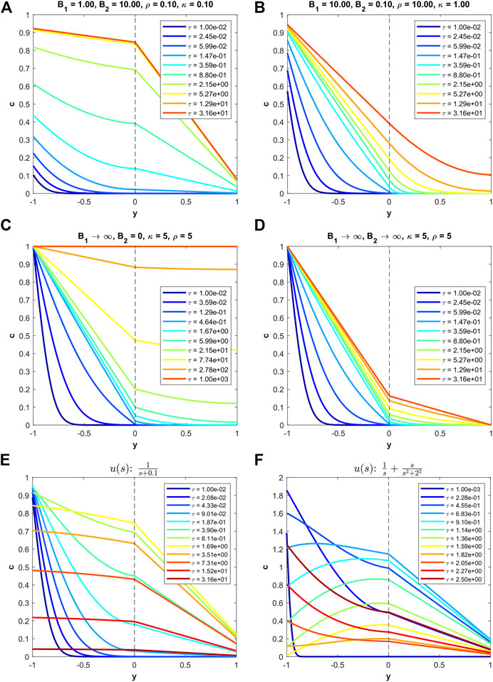
FIGURE 2. Examples of transient diffusion in a bi-layer with or without external mass transfer resistance. In (E) and (F), the input responses are time-varying and the properties of the composite are B₁ = 50, B₂ = 5, $\kappa =0.2$, and $\rho =0.2$.

2.2.2. Bi-Layer Diffusion With An Impermeable Wall at One End

There are a number of exact solutions that were previously derived for both the single-layer and bi-layer materials.

The simplified solutions assuming $B_1\to +\infty$ and $B_2\to 0$ are given by:

$c_1=1-{\displaystyle \sum }_{n=1}^{\infty }\frac{2\left(\text{cos}\left(\rho {\lambda }_n\right)\hspace{1em}\text{cos}\left(y_1{\lambda }_n\right)+\kappa \rho \sin \left(\rho {\lambda }_n\right)\hspace{1em}\text{sin}\left(y_1{\lambda }_n\right)\right)e^{-{\lambda }_n^2\tau }}{\left[\begin{array}{c}{\lambda }_n\left(\kappa {\rho }^2+1\right)\hspace{1em}\sin \left({\lambda }_n\right)\hspace{1em}\text{cos}\left(\rho {\lambda }_n\right)+\rho \left(\kappa +1\right){\lambda }_n\sin \left(\rho {\lambda }_n\right)\text{cos}\left({\lambda }_n\right)\\ +\kappa \rho \sin \left({\lambda }_n\right)\hspace{1em}\text{sin}\left(\rho {\lambda }_n\right)-\text{cos}\left({\lambda }_n\right)\text{cos}\left(\rho {\lambda }_n\right)\end{array}\right]}(55)$

and

$c_2=1-2\times {\displaystyle \sum }_{n=1}^{\infty }\frac{\rho {\lambda }_n\text{cos}\left(\rho {\lambda }_n\left(1-y_2\right)\right)e^{-{\lambda }_n^2\tau }}{\left[\begin{array}{c}{\lambda }_n\left(\kappa {\rho }^2+1\right)\hspace{1em}\text{sin}\left({\lambda }_n\right)\hspace{1em}\text{cos}\left(\rho {\lambda }_n\right)+\rho \left(\kappa +1\right){\lambda }_n\text{sin}\left(\rho {\lambda }_n\right)\hspace{1em}\text{cos}\left({\lambda }_n\right)\\ +\kappa \rho \sin \left({\lambda }_n\right)\hspace{1em}\text{sin}\left(\rho {\lambda }_n\right)-\text{cos}\left({\lambda }_n\right)\hspace{1em}\text{cos}\left(\rho {\lambda }_n\right)\end{array}\right]}(56)$

subject to the eigenvalues of:

$-\kappa \rho \text{sin}\left({\lambda }_n\right)\text{sin}\left(\rho {\lambda }_n\right)+\text{cos}\left({\lambda }_n\right)\text{cos}\left(\rho {\lambda }_n\right)=0.(57)$

Let’s note that the denominator of the large fraction in both concentration expressions can be further reduced to:

$\begin{array}{c}{c}_1=1-{\displaystyle \sum }_{n=1}^{\infty }\frac{2\left(\text{cos}\left(\rho {\lambda }_n\right)\text{cos}\left(y_1{\lambda }_n\right)+\kappa \rho \text{sin}\left(\rho {\lambda }_n\right)\text{sin}\left(y_1{\lambda }_n\right)\right)e^{-{\lambda }_n^2\tau }}{{\lambda }_n[\left(\kappa {\rho }^2+1\right)\text{sin}\left({\lambda }_n\right)\text{cos}\left(\rho {\lambda }_n\right)+\rho \left(\kappa +1\right)\text{sin}\left(\rho {\lambda }_n\right)\text{cos}\left({\lambda }_n\right)]}\end{array}(58)$

and

$\begin{array}{c}{c}_2=1-{\displaystyle \sum }_{n=1}^{\infty }\frac{2\rho {\lambda }_n\text{cos}\left(\rho {\lambda }_n\left(1-y_2\right)\right)e^{-{\lambda }_n^2\tau }}{{\lambda }_n[\left(\kappa {\rho }^2+1\right)\text{sin}\left({\lambda }_n\right)\text{cos}\left(\rho {\lambda }_n\right)+\rho \left(\kappa +1\right)\text{sin}\left(\rho {\lambda }_n\right)\text{cos}\left({\lambda }_n\right)]}.\end{array}(59)$

This solution not only assumes no flux at the downstream boundary but also that the transfer at the upstream boundary happens so quickly that the concentration there is essentially constant. We note here that, when compared with the previous work on this solution by Goldner et al. (1992), the eigenvalue expression (Equation 57) looks slightly different. In the attempt by the authors to simplify Equation 57 and divide the eigenvalue expression by $cos\left({\lambda }_n\right)cos\left(\rho {\lambda }_n\right)$, the authors omitted the possibility that, in some cases, the eigenvalues can lead to term containing the cosines to be 0, and thus leading to the tangent to be $+\infty$. However, this is only problematic in the scenario that such eigenvalue would also make $sin\left({\lambda }_n\right)$ or $sin\left(\rho {\lambda }_n\right)$ to be 0.

A representative example of this type of bi-layer is shown in Figure 2C. Most notably, the concentration is uniform across the bi-layer at steady-state. If B₁ is a finite value, then this steady-state concentration would be less than 1. The κ value of 5 here makes it such that the slope of the concentration in the first layer is sharper than the second layer. This difference, however, fades over time as the solution converges to steady-state.

2.2.3. Bi-Layer Diffusion With Constant Concentrations on Either Side

This derivation was previously presented in the work of Jaeger (1950). We simply show that by assuming that $B_1\to +\infty$ and $B_2\to +\infty$, equivalent expressions can be derived through simplifying the generalized bi-layer solutions:

$\begin{array}{c}{c}_1=\frac{-\kappa y_1+1}{\kappa +1}-{\displaystyle \sum }_{n=1}^{\infty }\frac{2}{{\lambda }_n}\frac{\left(\text{sin}\left(\rho {\lambda }_n\right)\text{cos}\left(y_1{\lambda }_n\right)-\kappa \rho \text{cos}\left(\rho {\lambda }_n\right)\text{sin}\left(y_1{\lambda }_n\right)\right)e^{-{\lambda }_n^2\tau }}{\left(\kappa {\rho }^2+1\right)\text{sin}\left({\lambda }_n\right)\text{sin}\left(\rho {\lambda }_n\right)-\rho \left(\kappa +1\right)\text{cos}\left({\lambda }_n\right)\text{cos}\left(\rho {\lambda }_n\right)}\end{array}(60)$

and

$\begin{array}{c}{c}_2=\frac{-y_2+1}{\kappa +1}-{\displaystyle \sum }_{n=1}^{\infty }\frac{2}{{\lambda }_n}\frac{\text{sin}\left(\rho {\lambda }_n\left(1-y_2\right)\right)e^{-{\lambda }_n^2\tau }}{\left(\kappa {\rho }^2+1\right)\text{sin}\left({\lambda }_n\right)\text{sin}\left(\rho {\lambda }_n\right)-\rho \left(\kappa +1\right)\text{cos}\left({\lambda }_n\right)\text{cos}\left(\rho {\lambda }_n\right)}\end{array}(61)$

with the eigenvalues provided by the roots of:

$\kappa \rho \text{sin}\left({\lambda }_n\right)\text{cos}\left(\rho {\lambda }_n\right)+\text{cos}\left({\lambda }_n\right)\text{sin}\left(\rho {\lambda }_n\right)=0.(62)$

An example of this well-known case is shown in Figure 2D. The main characteristics are that the upstream concentration is always 1, the downstream concentration is always 0.

2.2.4. Extension of the Step Response Solutions to Other Types of Input Responses

Using the Laplace expressions for both the single-layer and bi-layer systems, the derivation of other types of input (e.g., oscillatory, exponential decay, etc.) can be found trivially by factoring out $\frac{1}{s}$ from the expressions in Equations 19,20,43, and 44 and replacing it with the Laplace s-domain function representing the input of choice. Numerically inverting Laplace solutions into the time-domain can be done through various methods, some of which are outlined in Abate and Whitt (2006).

Alternatively, one can apply the truncated time domain convolution:

$\begin{array}{l}\left(f\ast g\right)\left(t\right)={\displaystyle \underset{0}{\overset{t}{\int }}f\left(\tau \right)g\left(t-\tau \right)d\tau }\hfill \\ forf,g:[0,\infty )\to \text{I}\text{R}.\hfill \end{array}(63)$

While the time-domain expressions may be convoluted in nature, the time-dependent elements of the solutions are relatively simple. Thus, the convolution can be straightforwardly calculated for many cases such as sine, cosine, or exponential inputs.

Two representative examples are shown in Figures 2E,F. In the first case (e) with $u\left(t\right)=e^{-0.1\tau }$, the exponential decay function starts at a high value, leading to an increase in concentration throughout the bi-layer. As the driving force of the input decays over time toward 0, the concentrations fall from high values around $\tau$ = 1.69 and eventually approaches 0 across the two layers. In the second case scenario with $u\left(t\right)=1+cos\left(2\tau \right)$, the behavior of the bi-alyer for a more complex input made up of a step function component and an oscillatory component is shown. This shows that the step function solutions can be easily adapted to handle more complex behaviors of the upstream “input” to the system.

2.2.5. Time Lag Analysis

The steady-state portion of m can be obtained from the steady-state portion of its transform, ${\text{lim}}_{s\to 0}\widehat{m}\left(s\right)$ as shown in Jaeger (1950). However, in this case, it remains quite challenging to derive for the bi-layer problem using that technique. Instead, the method outlined in Siegel (1991) is applied that makes analogies to the concepts in electrical engineering treating layers in a composite material like resistances in series. By assuming that the upstream and downstream boundaries are treated as layers of no thickness, the permeability P of the first and second layers take the following forms:

$\frac{1}{P^{\left(01\right)}}=1+\frac{1}{B_1},\frac{1}{P^{\left(23\right)}}=\frac{1}{\kappa }\left(1+\frac{1}{B_2}\right),(64)$

with ⁽⁰¹⁾ representing the first layer and ⁽²³⁾ representing the second layer. Using previous results that were obtained in the work of Siegel (1991), the time lags of the uncombined two layers are provided by:

${\tau }_L^{\left(01\right)}=\frac{1}{6}\left(1+\frac{2}{1+B_1}\right),{\tau }_L^{\left(23\right)}=\frac{{\rho }^2}{6}\left(1+\frac{2}{1+B_2}\right).(65)$

Let’s note that the time lags are nondimensionalized such that $\tau =\frac{D_{1}t}{L_1^2}$. The following expressions of forward mean first passage time of the second layer ${\overline{\tau }}_{+}^{\left(23\right)}$ (defined as ${\overline{\tau }}_{+}={\tau }_L-{\tau }_{+}$, with ${\tau }_{+}$ being the lead time)

${\overline{\tau }}_{+}^{\left(01\right)}=\frac{1}{2},(66)$

${\overline{\tau }}_{+}^{\left(23\right)}={\rho }^2\left(\frac{1}{2}+\frac{1}{B_2}\right),(67)$

as well as the backward mean first passage time of the first layer ${\tau }_{-}^{\left(01\right)}$ (defined as ${\overline{\tau }}_{-}={\tau }_L-{\tau }_{-}$, with ${\tau }_{-}$ being the backward lead time)

${\overline{\tau }}_{-}^{\left(01\right)}=\frac{1}{2}+\frac{1}{B_1}(68)$

are also introduced to derive the time lag of the bi-layer.

Applying the time lag (${\tau }_L$) expression for a series composite Siegel (1991),

${\tau }_L=\frac{\frac{{\tau }_L^{\left(01\right)}+{\tau }_{+}^{\left(23\right)}}{P^{\left(01\right)}}+\frac{{\tau }_L^{\left(23\right)}+{\tau }_{-}^{\left(01\right)}}{P^{\left(23\right)}}}{\frac{1}{P^{01}}+\frac{1}{P^{23}}},(69)$

the following expression for ${\tau }_L$ is obtained:

${\tau }_L=\frac{\left(1+\frac{1}{B1}\right)\left(\frac{1}{6}\left(1+\frac{2}{1+B_1}\right)+{\rho }^2\left(\frac{1}{2}+\frac{1}{B_2}\right)\right)+\frac{1}{\kappa }\left(1+\frac{1}{B_2}\right)\left(\frac{1}{6}{\rho }^2\left(1+\frac{2}{1+B_2}\right)+\frac{1}{2}+\frac{1}{B_1}\right)}{1+\frac{1}{B_1}+\frac{1}{\kappa }\left(1+\frac{1}{B_2}\right)}.(70)$

Similarly, the relationship in Siegel (1991) for the mean passage time in a bi-layer composite is provided by:

${\overline{\tau }}_{+}={\overline{\tau }}_{+}^{\left(01\right)}+{\overline{\tau }}_{+}^{\left(23\right)}+\frac{P^{\left(01\right)}}{P^{\left(23\right)}}[{\overline{\tau }}_{+}^{\left(01\right)}+{\overline{\tau }}_{-}^{\left(01\right)}](71)$

and

${\overline{\tau }}_{+}=\frac{1}{2}+{\rho }^2\left(\frac{1}{2}+\frac{1}{B_2}\right)+\frac{1}{\kappa }\left(1+\frac{1}{B_2}\right).(72)$

The lead time ${\tau }_{+}$ is then simply given by:

${\tau }_{+}={\tau }_L-{\overline{\tau }}_{+}.(73)$

Figure 3 shows the time lags for both the single-layer and bi-layer cases. In the single-layer case (a), which only depends on dimensionless parameters B₁ and B₂, an axis of symmetry (shown as a dotted white line) can be drawn across the heatmap. It indicates that the time lag for the single-layer system is independent as to whether the flow from the left to right or right to left. A similar observation to the invariance of the time lag with respect to flow direction can be made for the bi-layer system and is shown in (c) and (d). However, since the quantities κ, ρ, and ${\tau }_L$ are all dependent on how the layers are ordered. Given that ρ and κ are simply ratios between the first and second layer, one simply needs to take the reciprocal of these values to reverse the flow direction. For ${\tau }_L$, one needs to transform from the Fourier number of the first layer to that of the second layer, which can be simply done through dividing ${\tau }_L$ by ${\rho }^2$ or ${\tau }_L^{\prime }$ as in Figure 3D.

FIGURE 3

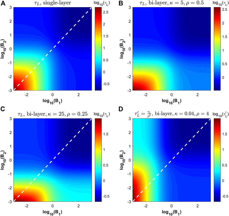
FIGURE 3. Heat maps of the dimensionless time lag ${\tau }_L$ for (A) the single-layer and (B,C) bi-layer membranes with changing B₁ and B₂ values. The effect of opposite direction for the permeate flux is shown in (D) for the same material properties described in (C).

In addition to the invariance to flow direction, it is also interesting to point out that the time lag is greatly affected by the values of B₁ and B₂. If both of these values are low, the time lag can be extremely large which coincides with the expected behavior that having large mass transfer resistance at the surfaces is not good for reaching steady-state permeation. This also shows that, depending on the values of κ and ρ in the bi-layer case, it may be easier to bring down the time lag by increasing one of the Biot number rather than the other. This can be seen in Figure 3C, for which it is easier to bring the time-lag down by increasing B₂. At the other end of the spectrum, high values for both B₁ and B₂ yield low time lag values.

In Figure 4, the steady-state and transient solutions for the dimensionless mass permeation expressions are combined for three different set of parameter values. The slopes of the asymptotes are provided by the time-domain concentration expressions in Equations 52 and 53. The lag time is provided by Equation 70 and the lead time is calculated using Equation 73 applied to Equation 71 and Equation 72. Evidently, the slope of the upstream and downstream steady-state solutions are the same since the flux coming into the membrane needs to exit at an equal rate or there would be accumulation within the bi-layer. This type of graph is important because, oftentimes, it is easier in practice to measure the mass permeated rather than the concentration value at a fixed location. Given time series data of the mass permeated, one can use the steady-state and transient solutions provided in this work to calculate missing membrane property values of the materials. In presented examples, it can be seen that the solution that reaches steady-state has high values of both B₁ and B₂, an observation that can also be seen in Figure 3. One can also use the slopes of the steady-state solutions to find missing values by noting, for example, that the steady-state slopes of the mass permeated expressions do not depend on κ and proceed through process of elimination.

FIGURE 4

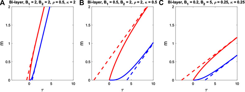
FIGURE 4. Examples of the time-dependent dimensionless mass permeated at the upstream (m_up, in red) and downstream (m_down, in blue) boundaries for three different bi-layer membranes.

3. Conclusion

There has been a large body of literature treating the problem of diffusion in n-layer composites. Yet, the derivation of closed-form solutions remain seldom and often limited to single-layer or bi-layer systems due to the difficult and tedious nature of finding such solutions. In this work, we presented analytical solutions to the phenomena of diffusion in a bi-layer with mass transfer resistance at the external boundaries for each of the layers as well as the corresponding expressions for the asymptotes of the upstream and downstream mass permeated. We showed how these relates to previously derived solutions of diffusion in a bi-layer with an impermeable wall as well as diffusion in a bi-layer with constant concentrations on either side. The step response solutions are also extended to time-varying inputs such as exponentially decaying and oscillating inputs. Notably, both the time-domain and Laplace domain solutions to the bi-layer can be used through numerical inversion of the Laplace solution or by applying a convolution on the provided time-domain solutions.

Also, the mean first passage time that is the difference between the lead and lag times does not depend on B₁. Since the lead time is dependent on the time lag, however, it is also dependent on all the four dimensionless quantities B₁, B₂, κ, and ρ. It was also shown that flipping the membrane materials around of the system has no bearing on the time lag for the single-layer and the bi-layer.

When comparing the generalized solutions with the simplified equations with constant concentrations on either side of the bi-layer membrane, there are notably two additional parameters in B₁ and B₂. It is likely that, in the absence of prior knowledge about the system, one cannot easily fit all the parameters at once from experimental data, especially when accounting for measurement errors. Knowledge about B₁ and B₂ can be derived most easily from studying the transient mass permeation in single-layer experiments of each of the components of the bi-layer. This is possible because the nondimensionalized lag time and the slope of the mass permeation in a single-layer membrane only depend on B₁ and B₂. Using experimental data from the bi-layer, one can, for example, use the fact that the slope of the mass permeation expressions are both independent of ρ. In this scenario, one can then use the lag time ${\tau }_L$ of the bi-layer to find κ. Real quantities of thickness, L₁ and L₂, are usually available or can be measured. Finally, the transient behavior that is provided by the derived equations of the generalized solutions to the bi-layer can be used to fit missing parameters. The objective of this work is to bring more insights as to how to characterize the permeation through bi-layers having non-negligible mass transfer resistances at its external boundaries by providing both the transient and steady-state analytical solutions.

Data Availability Statement

The original contributions presented in the study are included in the article, further inquiries can be directed to the corresponding author.

Author Contributions

JM conceptualized the initial idea of the paper. AT expanded these notes into a full manuscript and derived the equations presented here. ES provided help in the writing and support toward the completion of this work. All authors contributed to manuscript revision, read, and approved the submitted version.

Conflict of Interest

The authors declare that the research was conducted in the absence of any commercial or financial relationships that could be construed as a potential conflict of interest.

Acknowledgments

This manuscript could not have come to life without the contributions of JM. We hope that this work honors his memory, his passion for the field of heat and mass transport, and his dedication to nurturing the next generation of students and researchers. We also acknowledge the contributions of Kenneth A. Smith and Matthew J. Panzer for providing feedback on this manuscript.

References

Abate, J., and Whitt, W. (2006). A unified framework for numerically inverting laplace transforms. Inf. J. Comput. 18, 408–421. doi:10.1287/ijoc.1050.0137

CrossRef Full Text | Google Scholar

Al-Qasas, N., Thibault, J., and Kruczek, B. (2014). Analysis of gas transport in laminated semi-infinite solid: novel method for complete membrane characterization during highly transient state. J. Membr. Sci. 460, 25–33. doi:10.1016/j.memsci.2014.02.024

CrossRef Full Text | Google Scholar

Antonopoulos, K. A., and Tzivanidis, C. (1996). Analytical solution of boundary value problems of heat conduction in composite regions with arbitrary convection boundary conditions. Acta Mech. 118, 65–78. doi:10.1007/BF01410508

CrossRef Full Text | Google Scholar

Ash, R. (2001). A note on permeation with boundary-layer resistance. J. Membr. Sci. 186, 63–69. doi:10.1016/S0376-7388(00)00664-5

CrossRef Full Text | Google Scholar

Ash, R., Barrer, R., and Palmer, D. (1965). Diffusion in multiple laminates. Br. J. Appl. Phys. 16, 873. doi:10.1088/0508-3443/16/6/314

CrossRef Full Text | Google Scholar

Ash, R., Barrer, R., and Petropoulos, J. (1963). Diffusion in heterogeneous media: properties of a laminated slab. Br. J. Appl. Phys. 14, 854. doi:10.1088/0508-3443/14/12/307

CrossRef Full Text | Google Scholar

Barrer, R., and Rideal, E. K. (1939). Permeation, diffusion and solution of gases in organic polymers. Trans. Faraday Soc. 35, 628–643. doi:10.1039/TF9393500628

CrossRef Full Text | Google Scholar

Cabrera, M. I., and Grau, R. J. (2007). A generalized integral method for solving the design equations of dissolution/diffusion-controlled drug release from planar, cylindrical and spherical matrix devices. J. Membr. Sci. 293, 1–14. doi:10.1016/j.memsci.2007.01.013

CrossRef Full Text | Google Scholar

Cabrera, M. I., Luna, J. A., and Grau, R. J. (2006). Modeling of dissolution-diffusion controlled drug release from planar polymeric systems with finite dissolution rate and arbitrary drug loading. J. Membr. Sci. 280, 693–704. doi:10.1016/j.memsci.2006.02.025

CrossRef Full Text | Google Scholar

Cooper, E. R., and Kasting, G. (1987). Transport across epithelial membranes. J. Contr. Release 6, 23–35. doi:10.1016/0168-3659(87)90061-7

CrossRef Full Text | Google Scholar

Couto, A., Fernandes, R., Cordeiro, M. N. S., Reis, S. S., Ribeiro, R. T., and Pessoa, A. M. (2014). Dermic diffusion and stratum corneum: a state of the art review of mathematical models. J. Contr. Release 177, 74–83. doi:10.1016/j.jconrel.2013.12.005

CrossRef Full Text | Google Scholar

Crank, J. (1979). The mathematics of diffusion. Oxford, United Kingdom: Oxford University Press.

Google Scholar

Daynes, H. A. (1920). The process of diffusion through a rubber membrane. Proc. Math. Phys. Eng. Sci. 97, 286–307. doi:10.1098/rspa.1920.0034

CrossRef Full Text | Google Scholar

de Monte, F. (2002). An analytic approach to the unsteady heat conduction processes in one-dimensional composite media. Int. J. Heat Mass Tran. 45, 1333–1343. doi:10.1016/S0017-9310(01)00226-5

CrossRef Full Text | Google Scholar

de Monte, F. (2000). Transient heat conduction in one-dimensional composite slab. a natural analytic approach. Int. J. Heat Mass Tran. 43, 3607–3619. doi:10.1016/S0017-9310(00)00008-9

CrossRef Full Text | Google Scholar

Edil, T. B. (2003). A review of aqueous-phase VOC transport in modern landfill liners. Waste Manag. 23, 561–571. doi:10.1016/S0956-053X(03)00101-6

PubMed Abstract | CrossRef Full Text | Google Scholar

Forte, R., and Leblanc, J. (1992). New results on the kinetic aspect of the permeation resistance of elastomers, using an original testing cell and methanol as model permeating fluid. J. Appl. Polym. Sci. 45, 1473–1483. 10.1002/app.1992.070450816

CrossRef Full Text | Google Scholar

Frisch, H. L. (1957). The time lag in diffusion. J. Phys. Chem. 61, 93–95. doi:10.1021/j150547a018

CrossRef Full Text | Google Scholar

Frisch, H. L. (1958). The time lag in diffusion. II. J. Phys. Chem. 62, 401–404. doi:10.1021/j150562a005

CrossRef Full Text | Google Scholar

Frisch, H. (1959). The time lag in diffusion. IV. J. Phys. Chem. 63, 1249–1252. doi:10.1021/j150578a008

CrossRef Full Text | Google Scholar

Frisch, H., Damusis, A., and Hsieh, H. (1984). Film protection of polymers. J. Membr. Sci. 17, 255–261. doi:10.1016/S0376-7388(00)83217-2

CrossRef Full Text | Google Scholar

Garnier, G., Marouani, S., Yrieix, B., Pompeo, C., Chauvois, M., Flandin, L., et al. (2011). Interest and durability of multilayers: from model films to complex films. Polym. Adv. Technol. 22, 847–856. doi:10.1002/pat.1587

CrossRef Full Text | Google Scholar

Ghanem, A.-H., Mahmoud, H., Rohr, U. D., Borsadia, S., Liu, P., Fox, J. L., et al. (1987). The effects of ethanol on the transport of β-estradiol and other permeants in hairless mouse skin. ii. a new quantitative approach. J. Contr. Release 6, 75–83. doi:10.1016/0168-3659(87)90065-4

CrossRef Full Text | Google Scholar

Goldner, R. B., Wong, K. K., and Haas, T. E. (1992). One-dimensional diffusion into a multilayer structure: an exact solution for a bilayer. J. Appl. Phys. 72, 4674–4676. doi:10.1063/1.352072

CrossRef Full Text | Google Scholar

Gough, D. A., and Leypoldt, J. K. (1980). A novel rotated disc electrode and time lag method for characterizing mass transport in liquid-membrane systems. AIChE J. 26, 1013–1019. doi:10.1002/aic.690260617

CrossRef Full Text | Google Scholar

Gu, L., Wang, Y., Shi, S., and Dai, C. (2016). An approximate analytical method for nonlinear transient heat transfer through a metallic thermal protection system. Int. J. Heat Mass Tran. 103, 582–593. doi:10.1016/j.ijheatmasstransfer.2016.07.075

CrossRef Full Text | Google Scholar

Hatton, R. A., Blanchard, N. P., Miller, A. J., and Silva, S. R. P. (2007). A multi-wall carbon nanotube–molecular semiconductor composite for bi-layer organic solar cells. Phys. E Low-dimens. Syst. Nanostruct. 37, 124–127. doi:10.1016/j.physe.2006.07.001

CrossRef Full Text | Google Scholar

Jaeger, J. (1950). Conduction of heat in composite slabs. Q. Appl. Math. 8, 187–198. doi:10.1090/qam/36417

CrossRef Full Text | Google Scholar

Jaeger, J. C., and Carslaw, H. S. (1959). Conduction of heat in solids. Oxford, United Kingdom: Clarendon P.

Google Scholar

Jang, C., and Han, B. (2009). Analytical solutions of gas transport problems in inorganic/organic hybrid structures for gas barrier applications. J. Appl. Phys. 105, 093532. doi:10.1063/1.3116546

CrossRef Full Text | Google Scholar

Kalbe, U., Müller, W. W., Berger, W., and Eckardt, J. (2002). Transport of organic contaminants within composite liner systems. Appl. Clay Sci. 21, 67–76. doi:10.1016/s0169-1317(01)00093-x

CrossRef Full Text | Google Scholar

Laoubi, A., and Vergnaud, J. (1996). Processes of contaminant transfer into foods by diffusion-convection or by diffusion from packaging made of a recycled layer and a functional barrier. Polym. Polym. Compos. 4, 397–405.

Google Scholar

Levich, V. G. (1962). Physicochemical hydrodynamics. Prentice-Hall Inc.

Google Scholar

Liang, W., and Siegel, R. A. (2006). Theoretical and experimental exploration of rules for combining transport parameters in laminar membranes. J. Chem. Phys. 125, 044707. doi:10.1063/1.2216691

CrossRef Full Text | Google Scholar

Mikhailov, M. D., Özişik, M. N., and Vulchanov, N. L. (1983). Diffusion dans des couches composites et solution automatique du probleme des valeurs propres. Int. J. Heat Mass Tran. 26, 1131–1141. doi:10.1016/S0017-9310(83)80167-7

CrossRef Full Text | Google Scholar

Miller, J. R., and Weaver, P. M. (2003). Temperature profiles in composite plates subject to time-dependent complex boundary conditions. Compos. Struct. 59, 267–278. doi:10.1016/S0263-8223(02)00054-5

CrossRef Full Text | Google Scholar

Minelli, M., De Angelis, M. G., Doghieri, F., Rocchetti, M., and Montenero, A. (2010). Barrier properties of organic–inorganic hybrid coatings based on polyvinyl alcohol with improved water resistance. Polym. Eng. Sci. 50, 144–153. doi:10.1002/pen.21440

CrossRef Full Text | Google Scholar

Pollack, H. O., and Frisch, H. L. (1959). The time lag in diffusion III. J. Phys. Chem. 63, 1022. doi:10.1021/j150576a609

CrossRef Full Text | Google Scholar

Ramkrishna, D., and Amundson, N. R. (1974). Transport in composite materials: reduction to a self adjoint formalism. Chem. Eng. Sci. 29, 1457–1464. doi:10.1016/0009-2509(74)80170-3

CrossRef Full Text | Google Scholar

Rivero, S., García, M., and Pinotti, A. (2009). Composite and bi-layer films based on gelatin and chitosan. J. Food Eng. 90, 531–539. doi:10.1016/j.jfoodeng.2008.07.021

CrossRef Full Text | Google Scholar

Rutherford, S., and Do, D. (1997). Review of time lag permeation technique as a method for characterisation of porous media and membranes. Adsorption 3, 283–312. doi:10.1007/BF01653631

CrossRef Full Text | Google Scholar

Siegel, R. A. (1991). Algebraic, differential, and integral relations for membranes in series and other multilaminar media: permeabilities, solute consumption, lag times, and mean first passage times. J. Phys. Chem. 95, 2556–2565. doi:10.1021/j100159a083

CrossRef Full Text | Google Scholar

Smith, J. S., and Peppa, N. A. (1991). Mathematical analysis of transport properties of polymer films for food packaging. vii. moisture transport through a polymer film with subsequent adsorption on and diffusion through food. J. Appl. Polym. Sci. 43, 1219–1225. doi:10.1002/app.1991.070430702

CrossRef Full Text | Google Scholar

Subramanian, V. R., and White, R. E. (2001). New separation of variables method for composite electrodes with galvanostatic boundary conditions. J. Power Sources 96, 385–395. doi:10.1016/S0378-7753(00)00656-X

CrossRef Full Text | Google Scholar

Zhou, Y., and Wu, X. (2002). Theoretical analyses of dispersed-drug release from planar matrices with a boundary layer in a finite medium. J. Contr. Release 84, 1–13. doi:10.1016/s0168-3659(02)00263-8

CrossRef Full Text | Google Scholar