Modelling the Scaling-Up of the Nickel Electroforming Process

Introduction

Each one of the three industrial revolutions that have taken place so far present common characteristics which distinguish them from common, evolutional changes of the industrial sector. The main requirement for each one to take place has always been the accumulation of various innovations in industrial production. This is followed by up-dating infrastructure and the evolution of societies around a consequently transformed economy sector, producing new products, enhanced opportunities, as well as a reorganised production model. Eventually, the required resources and cost for production are reduced, product quality improves, niche products are developed. Finally, the real sector of economy reaches a new developed level of operation (Popkova et al., 2019).

Any industrial revolution that follows the previous three will also evolve in a similar way. In fact, the concept of the Fourth Industrial Revolution, which was introduced in 2011 (Slusarczyk, 2018), and published as a strategic plan for industrial development by two German Ministries in 2012 (Platform Industrie 4.0, 2012), required the accumulation of innovations in the sector of Internet of Things and Robotics, transition to fully automatised production lines, the development of new infrastructure able to support ultra-fast internet connections, the design and development of high-end robotic equipment, niche and cheap materials, significant decrease of the human factor in production, followed by an increased demand for highly specialised know-how (Popkova et al., 2019).

Even though “Industry 4.0” is not due soon, since the concept was introduced, most competitive industrial manufacturers around the world have been trying to secure sustainable, high quality, low cost technological developments. Using the continuously evolving and developing benefits that cyber-physical systems, the internet of things and artificial intelligence have to offer, the total computerisation of manufacturing and fabrication has been set as an aim (Müller et al., 2018). While these pillars of “Industry 4.0” would take care of the conversion of experimental data into digital format, to establish the smart factories of the future, processes themselves need to enter a new era. New manufacturing technologies will need to arise in order to replace traditional production lines with more flexible ones able to support the evolved industrial needs of this next transition.

Among these technologies, additive manufacturing processes have significantly contributed to the rapid transformation of the industrial landscape during the last decade (Ford and Despeisse, 2016). Much research has been focused on this new approach for fabrication, pointing out, not only the advantages but, also, the disadvantages derived from applying such methods and techniques. In particular, “low-volume/high-value” industrial sectors, such as the aerospace, marine and energy industries, are expected to benefit from this kind of approaches. This is mainly because manufacturing of larger volumes of customised products could be achieved in that manner. There could be a reduction of industrial and economic waste, which would decrease the cost of operation and reduce environmental impact. One such technology is electroforming.

Electroforming was first introduced as a technical process by the Prussian engineer and physicist, Moritz Hermann von Jacobi, in 1838. Since then, the process has been used in a wide range of applications; from fabrication of micro-components for medical and electronics sectors to the construction of large parts for aerospace industries, thereby impacting our daily life.

An appropriate definition would be, “electroforming is the production or reproduction of articles by electrodeposition upon a mandrel or mould that is subsequently separated from the deposit” (International, 2003) to be used as a standalone product. An electrochemical process requires at least two electrodes, an anode, and a cathode, to be immersed in an electrolytic solution, an electrolyte which contains the metal ions to be plated, and a power supply (DC) which enables current to flow through the system. The anode consists of the metal that is to be deposited on the mandrel while, the mandrel itself plays the role of the cathode and current collector. Due to voltage difference between the two electrodes, current passes between the anode and the cathode, leading to the conversion of metallic ions into atoms on the cathode’s surface.

From the mechanical engineer’s point of view, this is synonymous with an additive process because the atoms are being built up, layer by layer, until the desirable thickness of the electroformed part is achieved. As opposed to many academic studies in electrochemistry, the process is run using two electrodes in a galvanostatic fashion. The aspects which separate this process from normal electroplating is the fact that the formed part has to be separated from the substrate, which requires the form to have sufficient mechanical strength (John et al., 1999) as well as low internal stress (Kume et al., 2016) (Stein, 1996). These two requirements impose stringent limits on shape complexity, electrolyte choice and applied current density.

Even though nickel electroforms present exceptional mechanical properties and low to zero internal stresses (Committee B-8 Staff, 1962; Popereka, 1970; Uriondo et al., 2015; Davies and Jenkins, 2014; Jianhua et al., 2016; Zhu et al., 2006; Zhu et al., 2008; Li et al., 2019; Khazi and Mescheder, 2019) rendering electroforming a promising manufacturing process for “heavy” industries, our current knowledge base is derived predominantly from empirical data since scientific research has been limited. As it has been reported already (Roy and Andreou, 2020), although there is a huge volume of empirical data, more in-depth scientific analysis, amenable to predictive modelling, is needed. Most importantly, for volume manufacturing, systematic experimental and modelling investigations in the laboratory, and thereafter scaling-up to industrial conditions, are required. Such an approach would provide credible information which is currently not available.

Based on such information, certifiable models and new methodologies for controlling the thickness of an electroform, its uniformity and shape evolution could be developed. The authors have already discussed the state-of-the-art studies of modelling the electroforming process in a previous review paper (Andreou and Roy, 2021). However, it is important to briefly present here some of the most influential works—to the authors’ opinion—on modelling other metal electrodeposition processes, which have reported findings that are proven to be a potent starting point for the studies focusing on modelling the electroforming process itself.

In the 1980s Matlosz et al. investigated the secondary current distribution (SCD) in a Hull cell comparing the finite and boundary element methods for model development (Matlosz et al., 1987). Making the point that previous studies had mainly studied the primary current distribution (PCD) in deposition cells, they developed models and experimentally verified them to describe the SCD kinetics during copper deposition, ignoring the effects of mass transport phenomena. By assuming Butler-Volmer kinetics and studying both the Tafel and linear approximations, they reported a good agreement between the two computational methods and suggested that current density in a Hull cell can be described by a set of a Wagner number for Tafel kinetics, a Wagner number for linear kinetics and the anodic and cathodic Tafel slopes.

During the same decade the RDE was also used for secondary and tertiary current distribution (TCD) studies focusing on the co-deposition of nickel alloys (Ying et al., 1988) (Hessami and Tobias, 1989). By assuming Butler-Volmer kinetics to build their models, these studies investigated how process parameters like applied current densities, ion concentration and cathode surface pH affect the final product. To mention only some of their interesting suggestions, Ying et al. (Ying et al., 1988) succeeded in predicting their copper-nickel deposit composition as a function of the applied current, the process current efficiency and the polarisation data describing the experimental co-deposition process. Interestingly, they pointed out the difficulty in gathering data about hydrogen evolution during nickel deposition, arguing that the various reactions occurring in the process would not allow for accurate measurements. Consequently, they suggested that approximate predictions would only be possible through a “data force fitting” approach.

Hessami and Tobias (Hessami and Tobias, 1989) also investigated how agitation rate, electrolyte pH and hydrogen evolution affect deposit composition and process efficiency during the anomalous codeposition of nickel-iron alloys. Increasing agitation was reported to be in favour of iron deposition, linking that behaviour to higher hydrogen evolution at low potentials which reduces current efficiency. Another noticeable aspect is that increasing pH led to high nickel content at higher potentials and high iron content at low potentials. Through their observations and predictions, the authors confirmed once more the complex behaviour of anomalous co-deposition systems. Most importantly, however, and even though they reported good agreement between those observations and predictions, they established and pointed out the need for in-depth, systematic experimental studies before anomalous co-deposition processes could be sufficiently decoded.

Moving on to the next couple of decades, models were deployed to give answers to pressing electrodeposition-related questions considering various aspects of reactor and process optimisation. Aiming to overcome the Hull cell’s incapability during studies of processes dominated by a mass transport-limited step, Madore et al. (Madore et al., 1992a) developed a model in order to investigate primary and current distributions in a rotating cylinder Hull (RCH) geometry that they, themselves, had proposed months earlier (Madore et al., 1992b). Using the boundary element method (BEM) for their calculations and the Tafel approximation to describe the system’s kinetics, they calculated these distributions and established through experimental validation that their proposed cell could be successfully used for the study of various deposition processes, including alloy deposition.

On a different use of electrodeposition modelling, Krause et al. (Krause et al., 1997) took up the task of settling the argument between earlier models of Matlosz (Matlosz, 1993) and others’ (Romankiw, 1987; Grande and Talbot, 1993; Ramasubramanian et al., 1996) on the importance of ${\text{NiOH}}^{+}$ and ${\text{FeOH}}^{+}$ presence during nickel-iron co-deposition. To do so, Krause and his team proposed a reaction mechanism which involves ${\text{Ni}}^{+2}$ and ${\text{Fe}}^{+2}$ as the electroactive species instead and conducted $\text{NiFe}$ deposition experiments in a sulphate bath, using the RDE setup, to validate their predictions. Indeed, they succeeded in obtaining similar results with all the previously suggested models, proving that the presence of ${\text{NiOH}}^{+}$ and ${\text{FeOH}}^{+}$ species could be totally ignored. However, they highlighted the fact that none of the models could definitively be considered dominant over the others due to the tendency of transport models to include adjustable parameters which can be sensitive to variations in electrode preparation procedures, the electrodes’ working conditions or even the slightest differences in experimental approaches among different research groups.

In most recent years PCD, SCD and TCD studies are still a matter of interest for scientists and engineers worldwide. As new modelling tools become (commercially) available, new studies not only validate and update earlier modelling approaches, but also enrich already established models by incorporating complex phenomena with greater confidence. Using COMSOL Multiphysics® (formerly FEMLAB®), Low et al. (Low et al., 2007) modelled the copper electrodeposition from an acid sulphate electrolytic solution in an RCH cell with an offset anode developed by RotaHull® in early 2000s. Using the Tafel approximation to describe the system’s kinetics, assuming Nernstian behaviour for the diffusion layer, and taking into account even complex turbulent flow-related phenomena, they validated a novel setup and suggested, through simulations, the PCD’s dependence on the system’s geometrical characteristics, as well as a non-uniform current profile on the cathode’s surface. Furthermore, SCD simulated the real-life process more accurately under out-of-equilibrium conditions since it accounted for charge transfer, and it was observed to be valid far below the limiting current density. As a final step, TCD studies were run to determine the concentration, local current and overpotential profiles on the deposition surface and were used to describe their correlation.

Following an identical approach, Pérez and Nava (Pérez and Nava, 2014) investigated PCD, SCD and TCD in a rotating cylinder electrode (RCE) using four-plate, six-plate, and concentric cylinders as counter electrodes, under turbulent flow conditions. Their simulations were validated through copper deposition experiments. Their work provided an important insight into the behaviour of systems that use different counter electrodes and could potentially lead to more cost-effective and technically efficient cell systems.

Modelling of electrodeposition processes has also been useful to the study of industrial setups, especially ones with complex geometries and thus, complex electrode-electrolyte interactions. Such a case is the one of zinc electrowinning cells which Bouzek et al. (Bouzek et al., 1995) modelled in 1995. To simulate the case of an industrial electrowinning reactor the authors developed a model which was solving the Laplace’s equation for calculation of the potential and current distributions, the Tafel approximation to account for hydrogen and oxygen evolution and the Nernst equation to compute the equilibrium potentials needed for the analysis. Current efficiency was determined around an average of 85% due to impurities. Current distributions for the anodes and cathodes were also successfully computed. The model was validated for positioning of the cathodes’ active width between the anodes, since only the cathode position was varied experimentally. For other electrode arrangements the model was over-predicting the current density values. To account for such differences caused by the movement of a single cathode, an extended model consisting of three cathodes and two anodes was developed. Even then, however, inconsistencies between the experiments and simulations were observed. This model behaviour was attributed possibly to dendritic growth at the edges or, other, similar mass transport effects. At the same time, differences in predicted current densities between the regular and extended model revealed complex electrode interactions, with current travelling not only between a cathode and its neighbouring anode but also the second nearest one. As a general observation, moving the cathodes sideways was found to have much more effect on current distribution than positioning them at an angle with reference to the anodes. Also, the use of insulating edge strips at the cathodes’ edges led to significant non-uniformity in current distribution. To conclude, this work proposed a systematic approach for conducting geometry sensitivity studies, proving that careful reactor design could play an important role towards process optimisation.

Following a similar approach, Henquín and Bisang (Henquín and Bisang, 2009) studied current distribution in bipolar electrochemical reactors. Modelling the primary and secondary current distributions, they established that the latter is critically determined by a current leakage and an open bipolar stack, where the electrolyte is not constrained between the electrodes. Additionally, two different current paths were revealed, the expected one when current travels through the bipolar electrodes and a bypass when current travels around the electrodes rendering their overpotentials irrelevant to the process.

Last but not least, great attention has been paid recently in modelling the flow during electrodeposition under agitation. Modern modelling software has provided researchers with the ability to simulate fluid dynamics in reactor cells, incorporating into their models complex flow equations, minimising at the same time the need for overpowering assumptions and simplifications. Even though electrodeposition hydrodynamics have been the subject of modelling for many years now (Tribollet and Newman, 1983), computational fluid dynamics (CFD) analysis has been gaining significant ground during the last couple decades. Rivero et al. (Rivero et al., 2010) solved the Reynolds-averaged Navier-Stokes (RANS) equations to model a mass transport-controlled copper recovery process under turbulent conditions. They chose to study the process in an RCE and a six-plate counter electrode setup, establishing, among others, that dendritic formations can lead to an increase in micro-turbulence, as well as the fact that hydrogen evolution can be avoided under conditions of potentiostatic control for longer electrolysis when, eventually, mass transport takes control.

A similar methodology was also deployed more recently by Pérez et al. (Pérez et al., 2020) for modelling a laboratory-scale, filter-press flow cell for nickel electrodeposition. This time the authors aimed for reactor optimisation by conducting CFD studies to neutralise jet flow and edge effects on current density. They carefully considered the effects of hydrogen evolution during nickel deposition and observed that it takes place below $-0.4\text{ V}$. Consequently, they established that their SCD and TCD studies, conducted within a $(-0.4\text{ V})-(-0.7\text{ V})$ potential window, should indeed account for hydrogen evolution. Their proposed cell design was experimentally validated, suggesting that electrolyte manifolds followed by polymer meshes can significantly decrease edge effects on flow and current density. A “flow calming zone” was also introduced and established to be an effective addition to the reactor design.

Nevertheless, since most of the above discussed studies were conducted in the laboratory-scale, it is important to highlight the need for cautious adaptation of their findings to the inherent characteristics of large-scale additive manufacturing, including nickel electroforming for aerospace applications. To provide just a couple of examples, in these cases, it should be kept in mind that geometry sensitivity studies cannot be focused on simulating current distribution and/or mass transport phenomena for close electrode positions, as it is usually the case in laboratory-scale studies. Aerospace industry protocols determine the closest position that two electrodes could be placed at therefore, any effort to simulate real close electrode positions would not be of any use to industry.

However, it would be very useful, for example, to determine whether the anode position with reference to the cathode is “irrelevant” to the model. On another, rather dividing aspect, the need, or not, of modelling hydrogen evolution and tertiary current distribution should be considered cautiously. For one, even though specific processes (e.g., copper deposition) might easily result being affected by hydrogen evolution, this may not be the case for electroforming. In industry, nickel electroforming at currents between 5–20 ASD, using 100 L tanks under agitation, may be adequately described by SCD. In simulating such a process, therefore, the inherent characteristics of the system need to be considered to allow for comprehensive and informed modelling.

Approaching the issue from such a perspective and utilising the power of numerical analysis and the increasingly available computational resources, modelling the scale-up of an electroforming process could be used for making well-educated decisions on the limitations of an industrial-scale electroforming process. This would enable one to visualise the process conditions needed to obtain a particular electroform. A second consideration for such modelling is the availability of commercial software which can be implemented for an industrial process, and the limitations of such modelling tools.

In that effort, finite element methods (FEM) have been dominating the modelling studies of the electroforming process (Behagh et al., 2015) (Belov et al., 2016). The main reason is that it is the most efficient computational approach in sufficiently describing the boundary conditions and satisfactorily solving nonlinear electrochemical problems. A slightly different approach using BEM has also been used (Nouraei and Roy, 2007), where electrode shape changes, induced during a process, had to be taken into account. On one hand, finite element methods generally solve the current-potential equation throughout the electrolyte and the boundaries (i.e., cathode and anode), which may be slightly less efficient for the purposes of electrodeposition, electro-dissolution and electroforming where electrochemical reactions occur mainly at the boundaries. BEM, on the other hand, concentrates on evolving shape and associated changes in current and potential arising from these processes (Nouraei and Roy, 2007) (Elsyca, 2021). However, as computing power increases, computing efficiency is less of a problem, and hence FEM can be used to reasonably large-scale systems.

When it comes to scale-up modelling of processes with industrial interest, modellers should be able to comprehensively determine the way in which a model’s input parameters, geometric characteristics, and assumed physics, might be affected as the scale of a simulation increases. The inclusion of too many fitting parameters confounds engineering information, such as if size and shape of reactors (in the simplest case these are plating tanks) should be changed, current density should be increased or decreased or whether pulsating currents should be chosen (Wolfgang and Hansal, 2012), or how electrolyte–which influences electrode kinetics–should be chosen. In other words, the geometric and analytical limits of all models should be thoroughly researched and based on experimentally determined parameters, as far as possible, before any scaling up process is attempted. Nevertheless, such a research approach is missing nowadays, leaving important, scale-related, questions unanswered.

In an effort to shed light onto such a modelling methodology, which examines and elucidates the approach to resolving some of those uncertainties, this work consists of two parts. The first part includes geometry optimisation and model sensitivity studies of a 3-D electrodeposition model simulating the electroforming process on a laboratory-scale rotating disk electrode (RDE). This section involves the thorough examination of computational aspects of the model. The second part is focused on scaling-up to an industrial-scale process and compared against the RDE model. While an RDE-type system is seldom used in industry, the simplicity of the geometry allows one to explore issues arising due to scale up. In addition, for both the RDE as well as the industrial-scale system, experiments related to parameter determination and validation are reported here.

Geometry optimisation and model sensitivity studies were once more conducted for comparison purposes between the two scales. The key differences, challenges, and limitations during sizing upwards are reported here. For geometry optimisation studies, the relative position of the anode, with reference to the cathode position, and the cell size were varied for both the laboratory-scale and industrial-scale models. Additionally, the model sensitivity studies were focused on how the input parameters, process physics, mesh spacing, and computation times might be affected by the setup’s sizing-up.

COMSOL Multiphysics® was chosen for the studies presented in this paper. The software has been popular with electrochemists (Mahapatro and Suggu, 2018) (Heydari et al., 2020) and uses FEM for calculations. The authors have discussed the potential and limitations of the software in an earlier review (Andreou and Roy, 2021). In particular, it needs to be mentioned that our model used the “Electrodeposition” interface in COMSOL Multiphysics®. The system was set to work under galvanostatic mode (as is done in industry), the current at the cathode was determined, and the deposit thickness was calculated at each time step. This thickness was used to move boundary for the formed electrode as it evolved with time, and again the local currents were computed. The electrode reactions chosen were of Butler-Volmer type, with nickel and its ions being the only electroactive species. The physical dimensions of the reactor were used to fix reactor geometry. It is important to mention that COMSOL Multiphysics® can be installed in super-computers [e.g., Archie-West in Scotland (ARCHIE-WeSt, 2021)] as easily as in an average PC therefore it offers the possibility of studying scaled-up models of very large parts. This paper is based on results obtained using COMSOL Multiphysics® on a professional desktop.

Materials and Methodology

The laboratory-scale reactor was a $0.2\text{ L}$ double-wall electrolytic cell. The recessed RDE consisted of a $2\text{ M}$, industrial grade, $\text{Ni}{\left({\text{SO}}_3{\text{NH}}_2\right)}_2$ electrolytic solution, a 304 stainless-steel disk electrode ($\text{D }=0.12\text{ dm}$), and a nickel anode made out of industrial grade nickel pellets mounted on a titanium rod. The nickel sulphamate electrolyte is used for electroforming due to the deposits having good ductility, heat-resistance properties, high current-resistance properties and is related to low intrinsic stress (Baudrand, 1996). Since very low stress is required for aerospace applications, additives are not used, and these inherent characteristics of nickel sulphamate electrolytes are an advantage. The anode area was twice as that of the cathode to avoid anode passivation (Roy and Andreou, 2020). The disk electrode was rotating at 1,500 rpm. The electrolytic solution was heated by a water bath circulating water at $50\mathit{℃}$ through the cell’s jacket. Current was applied by a $1\text{ A}$ power supply through copper crocodile clips and deposits of $0.2\times {10}^{-3}\text{ m}$ (nominal) were deposited for verification of model computations. The RDE setup’s schematic is provided in Supplementary Figure S1 of this publication.

The $18\text{ L}$ tank reactor is made of polypropylene (PP) due to the material’s good mechanical properties at temperatures up to $80 \mathit{℃}$ and chemical resistance to dilute acids (Hindle, 2021). The system uses a SIEBEC MC15 pump and filter system to achieve sufficient electrolyte circulation. The M15 magnetic drive pump allowed for a maximum flow rate of $1.5{\text{m}}^3/\text{h}$ and particles between $0.5$ up to $150\text{ μm}$ were filtered using an on-line filter. A SIEBEC polypropylene $1/4^{\text{'}\text{'}}$ eductor nozzle was used to circulate the electrolyte within the tank. The electrolyte was heated by a $0.5\text{ kW}$ BRAUDE Polaris cylindrical non-corrodable heater. A BRAUDE Tankmaster MP temperature and level controller was used for continuous monitoring and controlling of the solution.

The anode basket and mandrels used in the process were immersed in the electrolyte by mounting them on $12\text{ mm}$ copper busbars of $>99\%$ purity. Current was applied by a $20\text{ A}$, $18\text{ V}$ RS PRO Switching DC Power Supply using $30\text{ A}$, steel, BU-65–0 Farnell crocodile clips. The anode basket was made of titanium and filled with industrial grade nickel pellets. The scaled-up disk mandrel ($\text{D}=0.63\text{ dm}$) was made of 304 stainless-steel. For the scaled-up experiments the same electrolyte as in the RDE experiments was used and deposits of $0.07\times {10}^{-3}\text{ m}$ (nominal) were deposited for verification of model calculations. The interior tank schematics are provided in Supplementary Figure S2 of this publication.

One needs to clarify here that the shapes and sizes of the laboratory-scale and tank reactors are dissimilar. This is intentional, because RDE are usually employed in laboratories, whereas a tank system is the “work horse” in industry. In the laboratory, glassware availability dictates the reactor shape, which is mostly cylindrical, whereas in industry plastic sheets are used to form more rectangular reactor structures.

Model Definition

The Finite Element Method

As per the definition given by Pepper and Heinrich in their book “The Finite Element Method: Basic Concepts and Applications” (Pepper and Heinrich, 2005), “the finite element method is a numerical technique that gives approximate solutions to differential equations that model problems arising in physics and engineering”. As in various finite difference schemes, the FEM requires a problem defined in a domain to be subdivided into a finite number of smaller elements, creating a mesh. For each one of the finite elements, the unknown variables are approximated using known functions. As a result, a set of finite linear equations is obtained, and linear algebra is used for solving these equations.

The mesh’s elements differ amongst one-, two- and multiple-dimension problems. Most commonly, in 1-D problems the elements appear as simple intervals, in 2-D problems as squares or triangles, while in 3-D problems can be either cubes or tetrahedrons (Berggren, 2012). For this arrangement to be valid, the end points of each triangle (element) edge should be at a vertex of the mesh, i.e., no “hanging nodes” should appear. The density of any mesh can be adjusted according to the problem’s needs.

Since every differential equation describing a problem is solved for each one of the mesh nodes, as a general principle, the differential equations involved will be solved more times within a fine mesh with more elements, compared to a coarse one. Consequently, more solutions, on more domain points, are calculated providing a better solution to the problem. As a result, the simulation’s final approximation will be closer to a “real” solution. At the same time, however, a longer computation time is needed for the model to achieve convergence.

Sensitivity studies of a model’s meshing tolerance could save valuable time since meshes of high node densities are not always needed for a model to return a reasonably accurate solution. This is usually done by manually reducing the mesh size (usually a 50% reduction in mesh size) and calculating the residual.

Once the residual size becomes independent of mesh spacing, very little would be gained from reducing the mesh size any further. A second method is using logarithmic mesh spacing, where the mesh is finest near the boundary or object of interest. However, the change in mesh spacing needs to be carefully handled due to computational issues and is often physics-controlled and calculated automatically by the software concerned.

In our simulations we maintained a user-controlled mesh spacing, finer near the electrode surface and determined by a parameter called the maximum element growth rate within the electrolyte domain. Specifically, this parameter was set at $1.1$ with reference to the finest elements present. This means that, with reference to and starting from the finest mesh elements, no element to follow can be bigger than 1.1 times any others adjacent to it. As a last step, obeying to that user-declared limitation, the software creates the mesh applying a free tetrahedral operation (Krusell, 2019).

Boundary and Initial Conditions

Following the mesh spacing of the domain, FEM is vitally dependent on the proper declaration of the problem’s initial and boundary conditions.

In the “Initial Values” node of the model builder, the user can define the starting values of the electrolyte potential (phil, as named in COMSOL Multiphysics®) and the electric (electrode) potential (phis, as named in COMSOL Multiphysics®). These values are simply starting guesses for the solver and they are mainly useful for stationary studies, providing a starting point for the solver. For time dependent studies, it is adviseable to use a “Current Distribution Initialization” study step prior to the main “Time Dependent” study step. The “Current Distribution Initialization” step defines new values for the initial values based on the primary assumption (fast kinetics). This sets the solver at a starting point closer to the solution, so that non-linearity in the kinetics do not cause convergence issues. For the purposes of this work $\mathbf{phil}$ and $\mathbf{phis}$ were set at the default 0 value while the “Current Distribution Initialization” study step was not needed for neither of the models discussed here, since convergence was easily achieved.

Moving forward, and as it can be understood, boundary conditions are derived from the physics of the problem. Most commonly, electrochemical systems generate non-linear, complex problems which are not easily formulated. To minimise the complexity of the problems, phenomena like migration and ion diffusion are usually being ignored, resulting in mathematical models less complicated and easy to handle.

Considering such simplifications being common, it is always more useful to focus on studying the behaviour of electrochemical systems and the functions that are used to describe the behaviour rather than the properties of the equations that might be chosen to define those functions. Consequently, potential theory i.e., the assumption that cell potential is solely governed by Laplace’s Equation 1.1, has always been an attractive approach to model an electrochemical problem. In that case, potential and current distributions are considered under the assumption that concentration is uniform throughout the domain (electrolyte volume). As long as the electrolyte’s composition remains uniform, that approach can be applied both for the cases when electrode kinetics are taken into consideration as is done in secondary current distribution (SCD) as well as for the case of primary current distribution (PCD) when no kinetics are considered (Newman and Thomas-Alyea, 2004).

Laplace’s Equation

${\mathbf{\nabla }}^2\mathbf{\phi }=\mathbf{0}$(1.1)

where $\mathbf{\nabla }=\mathit{i}\frac{\mathit{d}}{\mathit{dx}}+\mathit{j}\frac{\mathit{d}}{\mathit{dy}}+\mathit{k}\frac{\mathit{d}}{\mathit{dz}}$ and $\mathbf{\phi }$ is the local potential.

Taking it a step further from PCD when only the geometric characteristics of the electrochemical problem affect the calculations, SCD represents the results of more complex calculations taking place when slow electrode kinetics are taken into consideration and charge transfer is no longer neglected. In this case, the electrode’s surface is polarised to accommodate the overpotential to drive the current. Since an additional hindrance to the reaction, which, in effect is the kinetic resistance at the electrode-electrolyte interface, the Laplace’s equation solution is still possible but must include linear or logarithmic relations which are usually chosen to describe the relation between the surface overpotential and the potential derivative at the electrode. At insulators, no current can pass, and hence the conditions indicated as (1.2) below are obeyed.

$-\mathbf{n}\cdot {\mathbf{i}}_{\mathbf{l}}=\mathbf{0},-\mathbf{n}\cdot {\mathbf{i}}_{\mathbf{s}}=\mathbf{0}$(1.2)

In this work, the Butler-Volmer equation was used to mathematically describe the physics of the models investigated for this study. This model, amongst others, relates the surface overpotential to the reaction rate, which is the first fundamental information someone should know about any reactions taking place on the electrodes surfaces. Since the reaction rate is affected by the current density, the nature and quality of the electrode surface, the electrolyte, and the electrode potential, it is obvious that the correct determination of the model’s initial values and boundary conditions are of the utmost importance for the credibility of calculated values.

Butler-Volmer Equation

${\mathbf{i}}_{\mathbf{loc},\mathbf{m}}={\mathbf{i}}_{\mathbf{0},\mathbf{m}}\left({\mathbf{e}}^{\frac{{\mathbf{\alpha }}_{\mathbf{a},\mathbf{m}}\mathbf{F}{\mathbf{\eta }}_{\mathbf{m}}}{\mathbf{RT}}}-{\mathbf{e}}^{\frac{-{\mathbf{\alpha }}_{\mathbf{c},\mathbf{m}}\mathbf{F}{\mathbf{\eta }}_{\mathbf{m}}}{\mathbf{RT}}}\right)$(1.3)

where, for a given reaction $\text{m}$, ${\mathbf{i}}_{\mathbf{loc},\mathbf{m}}$ represents the local charge transfer current density, ${\mathbf{i}}_{0,\mathbf{m}}$ is the exchange current density, ${\mathbf{\alpha }}_{\mathbf{a},\mathbf{m}}$ and ${\mathbf{\alpha }}_{\mathbf{a},\mathbf{m}}$ are the anodic and cathodic charge transfer coefficients and, ${\mathbf{\eta }}_{\mathbf{m}}$ is the activation overpotential. $\mathbf{F}=96485.3 \mathbf{C}/\mathit{mol}$ is the Faraday’s constant, $\mathbf{R}$ is the universal gas constant and $\mathbf{T}$ the temperature under which the problem is studied. The term ${\mathbf{e}}^{\frac{{\mathbf{\alpha }}_{\mathbf{a},\mathbf{m}}\mathbf{F}{\mathbf{\eta }}_{\mathbf{m}}}{\mathbf{RT}}}$ is the anodic component of the B-V equation, and ${\mathbf{e}}^{\frac{-{\mathbf{\alpha }}_{\mathbf{c},\mathbf{m}}\mathbf{F}{\mathbf{\eta }}_{\mathbf{m}}}{\mathbf{RT}}}$ is the cathodic component.

In essence, eqn. 1.3 provides a summation of cathodic and anodic components of the dynamic electrode interface and provides an overpotential value which corresponds to an overall anodic or cathodic reaction. In this regard, for nickel deposition or dissolution at the cathode and anode boundaries, respectively, using the B-V expression shown in eqn. 1.3, one would compute positive (anodic) or negative (cathodic) values based on the overpotential experienced by it. Therefore, the B-V equation is applied to both the anode and cathode boundaries.

Actually, the exponential terms in the bracket represent anodic and cathodic parts of a single reaction at an electrode for a “fast” electrode reaction, whose limitations are discussed in forthcoming sections. A multi-step reaction, such as nickel deposition (Roy and Andreou, 2020), is more difficult to fit into a simple expression such as (1.3). In addition, the term outside the bracket on the right-hand side is dependent on concentration of the reactant. Parameters such as ${\text{α}}_{\text{c},\text{m}}$ and ${\text{α}}_{\text{a},\text{m}}$, again, are more difficult to ascertain if there are adsorbents, passivation or other parallel reactions occurring at the surface. However, for simplicity and validation, one can use an expression such as equation 1.3, and explore how well it can describe the process.

Before the model development is discussed in detail in the following section, it is worth commenting on the fact that, for this work, the mass transport phenomena developing during a metal deposition process were not taken into account. Instead, secondary current distribution was assumed to describe the problem. Although in many cases tertiary current distribution analysis can be employed, by choosing a Ni electroforming system, where applied current is approximately $10\text{\%}$ of that dictated by mass transfer limitations, one is able to scrutinise and assess a system which should be under kinetic control. Also, the use of high-concentration electrolytes and the vigorous mixing of the electrolytic solutions are two more reasons for one to follow such an approach.

This approach is also compatible with COMSOL’s proposed use of each one of the three current distribution interfaces available in the software (Pfaffe, 2014), providing additional confidence regarding the adequacy of the SCD interface to describe the problem’s physics. In any case, it is important to stress out that these studies are expected to help towards the process’s optimisation by, hopefully, providing an insight into complex phenomena controlled by reactor geometry and reaction kinetics. Since TCD may not provide additional information during reactor scaling-up and geometry optimisation studies, which are the main point of focus of the work presented here, the models to follow are SCD cases.

A Note on Convergence

As a general description, in COMSOL Multiphysics® a time-dependent solver computes a solution to a nonlinear system of equations at each timestep applying a set of iterative techniques based on Newton’s method. Such solving techniques assess a function and its derivative at all timesteps. This derivative is known as the Jacobian and it requires high computational power to be determined. To overcome this issue the software always tries to minimise re-assessing the Jacobian each time. In case convergence cannot be reached, it reduces the user-defined timestep size and tries to compute the solution again. This is an efficient approach for the cases when solution fields change rapidly with time.

When COMSOL’s default “Constant (Newton)” nonlinear method is applied, non- convergence issues can be addressed by updating the Jacobian on every iteration that the nonlinear solver takes as it tries to compute the solution at each timestep. If this is not enough, in case the problem is so strongly nonlinear that the “Constant (Newton)” method can not still converge, there are other settings a user can modify; increase the “Maximum number of iterations” from the default value of 4 to 25 or higher, or even adjust the “Tolerance factor” to a more relaxed one. If the model is still not converging, the “Constant (Newton)” method can be changed to “Automatic (Newton)” which updates the Jacobian and uses a dynamic damping term. This method will require more computational power. As a last resort, the “Automatic highly nonlinear (Newton)” method can also be applied. This approach will be slower, but more likely, to converge since it starts with higher damping. For the purposes of this work the “Automatic (Newton)” nonlinear method was applied, with a maximum number of iterations at 4 and tolerance factor at 1.

Once the current has converged, the thickness of the electroformed layer is calculated using the Faraday’s Eqn. 1.4:

$\mathbf{T}\mathbf{h}i\mathbf{c}\mathbf{k}\mathbf{n}\mathbf{e}\mathbf{s}\mathbf{s} \mathbf{o}\mathbf{f} \mathbf{N}\mathbf{i} \mathbf{p}\mathbf{l}\mathbf{a}\mathbf{t}\mathbf{e}\mathbf{d}={\displaystyle \sum _{\mathbf{t}=\mathbf{0}}^{\mathbf{t}=\mathbf{d}\mathbf{t}}{\mathbf{i}}_{\mathrm{l}\mathrm{o}\mathrm{c}}}\times \frac{\mathbf{M}{\mathbf{r}}_{\mathbf{N}\mathbf{i}}}{\mathbf{n}\mathbf{F}\mathbf{A}{\mathbf{\rho }}_{\mathbf{N}\mathbf{i}}}\times \mathbf{t}$(1.4)

where, ${\displaystyle \sum }_{\mathbf{t}=0}^{\mathbf{t}=\mathbf{dt}}{\mathbf{i}}_{\mathbf{loc}}$ is the total current, $\mathbf{M}{\mathbf{r}}_{\mathbf{Ni}}$ the molar weight of nickel, $\mathbf{A}$ the surface of the deposited area and ${\mathbf{\rho }}_{\mathbf{Ni}}$ the density of nickel.

The new boundary is then set at the surface of the newly formed layer, which is then the boundary for the subsequent calculation.

The COMSOL Multiphysics® model (s)

A time-dependent 3-D model of a recessed rotating disk electrode (RDE), laboratory-scale, $0.2\text{ L}$, system was developed within the Electrodeposition module of COMSOL Multiphysics®. A second time-dependent model was, subsequently, developed to represent a scaled-up, $18\text{ L}$, electroforming reactor. The 3-D geometries for the laboratory-scale RDE and the scaled-up electroforming reactor are shown in Figures 1A,B. Both electroforming systems consist of a cathode and an anode immersed in the electrolytic volume. A stainless-steel disk $\sim 0.12\text{ dm}$ in diameter $\left({\text{A}}_{\text{RDE}}=\sim 0.0113{\text{ dm}}^2\right)$ was used as the deposition substrate (cathode) for the RDE (Figure 1C). In the scaled-up system a stainless-steel disk $\sim 0.63\text{ dm}$ in diameter $\left({\text{A}}_{\text{mandrel}}=0.31{\text{ dm}}^2\right)$ playing the role of the mandrel (cathode) (Figure 1D) was used. In both cases the (cathode area): (anode area) ratio is always kept greater than $1:2$ as is practised in industry. When compared, the two systems present 1:90 elecrolyte volume ratio and a 1:28 deposition (cathode) area ratio. The difference in areal and volumetric ratios is expected as per dimension analysis due to the fact that they scale as ${\left(\text{length}\right)}^2$ or ${\left(\text{length}\right)}^3$.

FIGURE 1

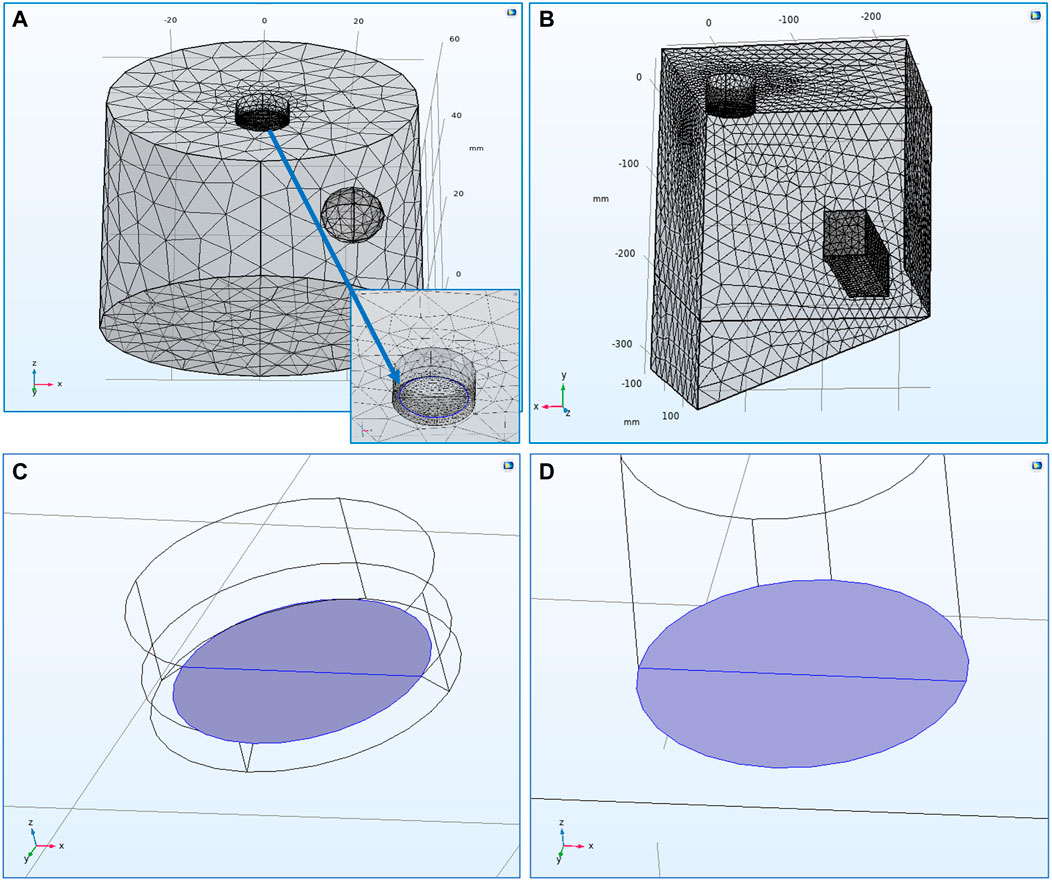
FIGURE 1. (A) Mesh spacing of the 3-D, laboratory-scale $\left(0.2 d{m}^3\right)$, RDE geometry domain and (B) mesh spacing of the 3-D, industrial-scale $\left(18 d{m}^3\right)$, prototype electroforming reactor domain. The blue line in the zoom-in capture of figure (A) highlights the “recess”, transition edge of the stainless-steel disk electrode in the RDE model. The deposition (cathode) areas of (C) the laboratory-scale setup and (D) the scaled-up setup are also shown. The electrolytic volumes present a ration of 1:90 and the deposition areas a ratio of 1:28.

As has been described before, the first part of developing a model in COMSOL Multiphysics® is an efficient mesh generation for the model’s domain and electrode surfaces. A user-defined mesh spacing was chosen for both models.

Within COMSOL Multiphysics® mesh quality is controlled by a series of mesh quality measures, including, but not limited to, elements’ maximum angle, volume versus length ratio and growth rate. For this work, skewness was used as the element quality measure which is the default quality measure. Skewness is a “measure of the equiangular skew which is defined as the minimum of the following quantity:

$\mathbf{1}-\mathbf{max}\left(\frac{\mathbf{\theta }-{\mathbf{\theta }}_{\mathbf{e}}}{\mathbf{180}-{\mathbf{\theta }}_{\mathbf{e}}},\frac{{\mathbf{\theta }}_{\mathbf{e}}-\mathbf{\theta }}{{\mathbf{\theta }}_{\mathbf{e}}}\right)$

where θ is the angle over a vertex (2D) or edge (3D) in the element, θe is the angle of the corresponding edge or vertex in an ideal element, and the minimum is taken over all vertices (2D) or edges (3D) of the element” (Comsol, 2021). Element quality is a dimensionless parameter taking values between 0 and 1 and refers to the elements’ regularity; 0 corresponds to degenerated elements and 1 to perfectly regular ones. Any value below 0.1 describes poor quality elements. In fact, automated warnings will be generated by the software when elements of quality below 0.01 are generated since those must be fixed to avoid convergence issues.

Figures 1A,B show the mesh spacing of both models and highlight the points of interest mentioned above. Since the main interest is focused on the deposits formed on the cathode’s surface, the mesh on the cathode boundary was the finest in both models. For the RDE, special attention was given on the “recess” region at the border between the cathode and insulation surface at the RDE tip (Figure 1A). Since this border is considered as a transition edge, the mesh there was generated to be really fine in order to avoid any mesh deformation phenomena which could prevent the model from converging. The mesh developed for the RDE model included 17,255 elements with minimum element quality of 0.2149. On the other hand, the scaled-up model included 132,291 elements with minimum element quality of 0.2045 to accommodate the larger domain. Therefore, both models’ meshes were developed to present similar average element qualities; 0.652 for the RDE model and 0.6603 for the scaled-up one.

As a next step, within this software one needs to choose the system, i.e., PCD or SCD, so that the boundary conditions and the (electro) chemical input parameters can be declared. For this work secondary current distribution (SCD) was chosen to describe the process physics. The electrochemical input parameters needed to describe the electrochemical system were determined experimentally in the laboratory. Table 1 summarises the boundary conditions and input parameters required by the software to successfully run the simulations, and a detailed discussion on the Ni reaction is also included towards the end of this section.

TABLE 1

TABLE 1. Physical and (electro)chemical model input parameters.

Secondary current distribution is the suggested COMSOL Multiphysics® interface for modelling industrial electrochemical processes (Pfaffe, 2014). This interface should be used to model processes where there is sufficient agitation or high concentration of reactant ensuring the reacting species at the electrode surface are same as that in the solution. Industrial electroforming takes place under intense agitation and the nickel sulphamate concentration in the electrolyte is high. In such processes, concentration overpotential can be neglected but the losses caused by electrode polarisation are not negligible compared to ohmic drop, and SCD conditions can be assumed to prevail.

In SCD the concept of the activation overpotential ($\text{η}$) is introduced. As soon as electrode kinetics are introduced in the models, the potential of the electrode in question differs from the equilibrium value due to resistance attributed to the rate of the electrolysis reaction. This difference between the actual potential and that at equilibrium is the activation overpotential ($\text{η}$), which, in reality, drives the electrode reaction. Within COMSOL Multiphysics® the inclusion of activation overpotential is handled in the following fashion. The current is related to the potential at the electrode surface, ${\mathbf{\phi }}_{\mathbf{s}}$, by

${\mathbf{i}}_{\mathbf{s}}=-{\mathbf{\sigma }}_{\mathbf{s}}\nabla {\mathbf{\phi }}_{\mathbf{s}}$(1.5)

and the current is related to the potential in the electrolyte, ${\mathbf{\phi }}_{\mathbf{l}}$, by

${\mathbf{i}}_{\mathbf{l}}=-{\mathbf{\sigma }}_{\mathbf{l}}\nabla {\mathbf{\phi }}_{\mathbf{l}}$(1.6)

where, ${\mathbf{i}}_{\mathbf{s}}$ and ${\mathbf{i}}_{\mathbf{l}}$ are the local current densities at the electrode surface and the electrolyte immediately next to the surface, respectively. Based on the overpotential, the electrolyte-electrode interface will be described by Eqn. 1.7:

${\mathbf{\eta }}_{\mathbf{m}}={\mathbf{\phi }}_{\mathbf{s}}-{\mathbf{\phi }}_{\mathbf{l}}-{\mathbf{E}}_{\mathbf{eq},\mathbf{m}}$(1.7)

Notably, ${\mathbf{\phi }}_{\mathbf{s}}$ is the local potential at the electrode, ${\mathbf{\phi }}_{\mathbf{l}}$ is the local potential in the electrolyte and, ${\mathbf{E}}_{\mathbf{eq},\mathbf{m}}$ is the equilibrium potential for the reaction $\text{m}$.

The SCD interface uses relations between current density and overpotential at each location to solve any given problem. As it was mentioned before, the Butler-Volmer Eq. 1.3 is one of these equations and is included as an option in COMSOL Multiphysics®.

The total current on the electrode-electrolyte interface of both electrodes is expressed by Eqn. 1.8:

$-{\mathbf{i}}_{\mathbf{s}}\cdot \mathbf{n}={\mathbf{i}}_{\mathbf{l}}\cdot \mathbf{n}={\displaystyle \sum _{\mathbf{m}}{\mathbf{i}}_{\mathbf{loc},\mathbf{m}}}$(1.8)

where, $\mathbf{n}$ is the number of the currents of all the reactions occurring on the electrode surface.

The conditions used for both the RDE, and electroforming reactor models were chosen based on practical experiments conducted in both a laboratory-scale, RDE ($0.2\text{ L}$) and an industrial-scale, prototype electroforming reactor ($18\text{L}$) setup (Supplementary Figures S1, S2). All simulation experiments were designed to represent practical deposition experiments, at $50\mathrm{℃}$, for $3\text{ h}$, when the cell voltage lies at $2.5\text{ V}$. Since electrolyte’s nickel concentration is high, no concentration gradients need to be taken into consideration therefore, to simplify the calculations, no mass transfer limitations were considered.

Ni Reduction Reaction

It has been proposed Ni reduction reaction to occur through the following steps (Roy and Andreou, 2020), of which the rate determining step (RDS) is Eqn. 1.10:

${\mathrm{Ni}}^{2+}+{\mathrm{H}}_{\mathrm{2}}\mathrm{O}\leftrightarrow \mathrm{N}\mathrm{i}{\left(\mathrm{O}\mathrm{H}\right)}^{+}+{\mathrm{H}}^{+}$(1.9)

$\mathrm{Ni}{\left(\mathrm{O}\mathrm{H}\right)}^{+}+{\mathrm{e}}^{-}\leftrightarrow \mathrm{N}\mathrm{i}{\left(\mathrm{O}\mathrm{H}\right)}_{\mathrm{ads}}$(1.10)

$\mathrm{Ni}{\left(\mathrm{O}\mathrm{H}\right)}_{\mathrm{a}\mathrm{d}\mathrm{s}}+{\mathrm{e}}^{-}\leftrightarrow \mathrm{N}\mathrm{i}+\mathrm{O}{\mathrm{H}}^{-}$(1.11a)

or

$\mathrm{Ni}{\left(\mathrm{O}\mathrm{H}\right)}_{\mathrm{a}\mathrm{d}\mathrm{s}}+\mathrm{N}{\mathrm{i}}^{2+}+2{\mathrm{e}}^{-}\leftrightarrow \mathrm{N}\mathrm{i}+\mathrm{N}\mathrm{i}{\left(\mathrm{O}\mathrm{H}\right)}_{\mathrm{a}\mathrm{d}\mathrm{s}}$(1.11b)

Experimentation has shown that Tafel slopes range between 0.090 V decade-1 and 0.200 V decade-1 (Tsuru et al., 2002), which lends some support to this proposition. However, including such complex kinetics in standard COMSOL software is non-trivial, because the system allows for simple Butler-Volmer type of kinetics. Indeed, it is difficult to incorporate electrode kinetics which depend on the number of surface sites, when there are three electrode reactions, or the surface sites change with electrode polarisation. Therefore, one has to make some simplifications and, for convenience, the overall reaction, as shown in Table 1, is considered in our model.

An experimental polarisation curve was measured in the laboratory RDE setup by linear sweep voltammetry with a scan rate of $0.005\text{V}/\text{s}$, at $50{ }^{°}\mathrm{C}$ and under agitation at $1500\text{ rpm}$. Based on the current-potential curve obtained experimentally, the system's electrochemical parameters were determined at $\text{n}=2$, ${\text{a}}_{\text{c},\text{m}}=0.194$, ${\text{a}}_{\text{a},\text{m}}=1.806$ and ${\text{i}}_0=0.42\text{ A}/{\text{dm}}^2$. The theoretical value for nickel is ${\text{E}}_{\text{eq},\text{ Ni}}=-0.26V$. However, our laboratory data, shown in Figure 2 in red, suggest slow kinetics for nickel reduction kinetics, especially with a large overvoltage $\left({\text{E}}_{\text{eq},\text{ Ni}}\equiv {\text{E}}_{\text{rev}}=-0.82V\right)$ before any current is observed.

FIGURE 2

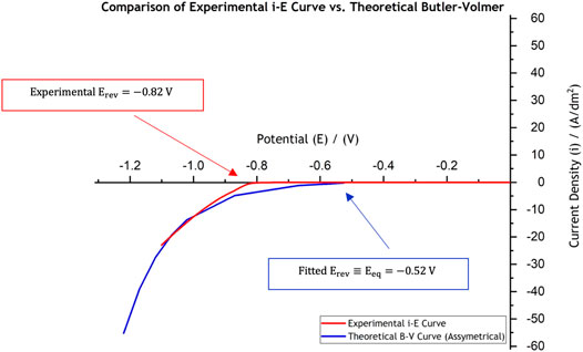
FIGURE 2. Comparison of the experimentally collected data in the laboratory using linear sweep voltammetry (red curve) against the theoretical current-potential behaviour for use in Ni electroforming models, “shifted” B-V curve (blue line). The linear sweep voltammetry was conducted at a scan rate of $0.005\text{V}/\text{s}$, $50 \mathit{℃}$ and under agitation at $1500\text{ rpm}$. The kinetic parameters used to plot the theoretical Butler-Volmer curve were the ones presented in Table 1. $\left[1\text{A}/{\text{dm}}^2=100\text{ A}\cdot {\text{m}}^{-2}\right]$.

The theoretical current-potential (B-V) curve, based on the parameters extracted from the experimental curve (red curve in Figure 2) and which are presented in Table 1, is also shown in Figure 2 in blue. One important difference between the experimental data (red curve) and the fitted curve (blue one) is the large inactive region extending between $0$ and $-0.82\text{ V}$ for the experimental curve and between $0$ and $-0.52\text{ V}$ for the fitted theoretical B-V curve. In effect, the reversible potential used to fit the current-potential data is $-0.52\text{ V}$. This is different from the nickel theoretical thermodynamic value of ${\text{E}}_{\text{eq},\text{ Ni}}=-0.26\text{ V}$. Although this difference may not incorporate an error in computation of current values, it will leave an uncompensated potential drop of $0.3\text{ V}$, which appears in lower values of cell potential in computations. A second difference between the experimental data is observed at current densities lower or higher than the region where the data was used to fit the current. However, since most electroforming experiments are carried out at current densities in the region of interest where theoretical and experimental data match, the computed values should provide reasonable values for current distribution across the electrode surface.

Some models on nickel plating include hydrogen evolution reaction (Ying et al., 1988) (Hessami and Tobias, 1989). However, this is not a requirement for electroforming models, because hydrogen evolution constitutes less than 1% of the applied current. This means that even if the hydrogen reduction reaction was included in the model, experimental B-V parameters could not be collected, and hence, the validity of hydrogen evolution can never be tested.

Results and Discussion

Control Simulations

For the “control” simulation experiments, in the RDE model the cathode phase condition was described by a total applied current (${\text{I}}_{\text{l},\text{total}}$) at $-0.0372\text{ A}$ and an applied boundary electric potential (${\text{φ}}_{\text{s},\text{ext},\text{init}}$) at $-2.5\text{ V}$ (note that, in COMSOL Multiphysics® terminology, “electric potential at the electrode boundary” means “electrode potential”). Similarly, for the industrial-scale model the boundary condition at the cathode was described by a total current $\left({\text{I}}_{\text{l},\text{total}}\right)$ at $-1 A$ and an electric (or electrode) potential initial value (${\text{φ}}_{\text{s},\text{ext},\text{init}}$) at $-2.5\text{ V}$. Anode boundary conditions were set at $0\text{ V}$ for both models to achieve $2.5\text{ V}$ cell voltage in both cases. In terms of current density, the above stated values correspond to deposition at $3.2\text{ A}/{\text{dm}}^2$ in both scales, a value representative of those used for nickel deposition in industry (Roy and Andreou, 2020).

Figure 3 shows the current and potential distribution results for the two models after the simulation had converged. The visualisation in Figures 3A,B allows one to check the potential distribution in the domain and near the electrode surface as well as the current lines travelling to the electrode surface. Control simulations showed that the potential drop within the electrolyte is different for the two models; $0.29\text{ V}\leftrightarrow 0.51\text{ V}$ for the RDE system and $-0.41\text{ V }\leftrightarrow 0.52\text{ V}$ for the tank apparatus. . The maximum potential value immediately next to the anodes is the same (i.e., 0.52 V as would be expected for dissolution to proceed), while the potential near the cathode surface is different for the two systems. This difference is induced by the reactor boundaries; not only do the current lines bend away from the insulator walls since no current can pass through them, thereby leading them towards the cathode surface, but also through the different lengths of the current lines have to travel as they move through the electrolyte. Indeed the surface potential at the cathode for the RDE and electroforming reactor differ due to the larger ohmic drop for the latter system.

FIGURE 3

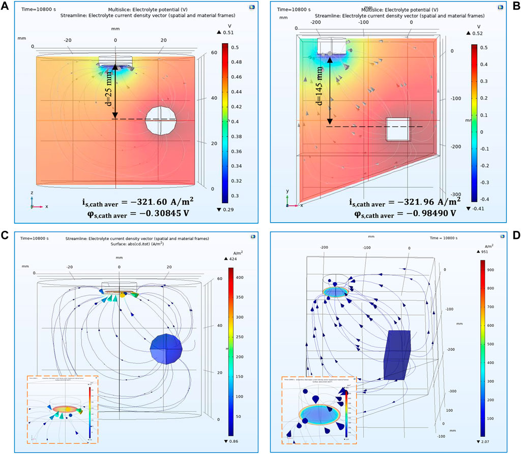
FIGURE 3. 3-D representation of potential distribution in the electrolyte volume of (A) the RDE and (B) the electroforming reactor. 3-D representation of current distribution on the cathode surface for (C) the RDE and (D) the electroforming reactor. The results simulate potential and current distributions after $3h$ at $50 \mathit{℃}$. The current streamlines in both electrolytic volumes are also shown in figures (C,D) emanating from the anode (at higher potential) and being collected at the cathode (at lower potential). The vertical distance between the electrodes’s geometrical centres is also noted in figures (A,B). Current distribution on the cathodes’ surface is shown in the cathode surface close ups provided in figures (C,D).

To verify the predicted system behaviour the value of the local potential at the cathode surface was followed. This is important since it is the convergence parameter with reference to which both models conduct the calculations; indeed, the total current and anode potential remain fixed, and the cathode surface local potential (${\text{φ}}_{\text{s}}$) is adjusted by the model to calculate the local current density, which is then summed up to obtain the total current density, and compared against the value set for the simulation.

Both models are time-dependent therefore, due to the surface evolution of the formed electrode, the cathode surface changes with time as new layers of nickel are deposited. The model was set to record a solution every 30 min (1800 s) therefore, 7 time steps were set. The model was solved to provide convergent solutions varying between t = 0 (for a non-evolved surface) and the last for t = 10,800 s (for an evolved surface where a deposit was formed), reflecting deposition for 3 h.

In this regard, after the final converged time step, the local average cathode surface potential was determined at ${\text{φ}}_{\text{s},\text{cath aver}}=-0.30845\text{ V}$ for the RDE and ${\text{φ}}_{\text{s},\text{cath aver}}=-0.98490\text{ V}$ for the scaled-up system. Although there is a slight change in the electrode surface potential due to the evolution of the deposit (i.e., that the cathode boundary had changed) the effect is small. The essential difference between the two systems is the difference in scale, leading to very different ohmic drops, and hence cathode potentials do not vary.

By comparing these local potential values within the electrolyte immediately next to the cathode, i.e., ${\text{φ}}_{\text{l},\text{local}}$, one can ascertain the energy needs due to ohmic drop for this process. Here, as indicated in Figures 3A,B, the distance between the cathode’s surface and the (centre of) anode lies at $25\text{ mm}$ for the RDE model and $145\text{ mm}$ for the scaled-up one. At the same time, the cathode surface local potential in the tank system model is calculated to be three times higher than the one at the RDE cathode surface, i.e., the longer distance between the electrodes results in higher energy requirement for the process to be driven. The calculated current density values range from $0.86\text{ A}/{\text{m}}^2$ to $424\text{ A}/{\text{m}}^2$ at the cathode surface for the RDE while, they range between $2.07\text{ A}/{\text{m}}^2$ and $951\text{ A}/{\text{m}}^2$ for the electroforming reactor conditions in Figures 3C,D.

Moving forward, Figure 4 presents the deposit thickness profiles (reflecting the current distribution) predicted for the two different reactors. In general, the current is predicted to be higher at the edges than at the centre of the disk as would be expected (Andreou and Roy, 2021). Consequently, increase in thickness profiles was predicted at the edges. In Figure 4A, the model shows that the overall thickness distribution (reflecting the current distribution) follows the usual non-uniform current distribution as expected for an RDE; however, the low current at the insulator-RDE edge is caused due to the shadowing effect of the recess (Dinan et al., 1991). The current distribution for the cathode (mandrel) within the electroforming reactor (Figure 4B), on the other hand, shows typical non-uniform thickness distribution, with high current at the edges and lower current at the centre.

FIGURE 4

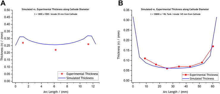
FIGURE 4. Comparative graphs of the experimentally achieved and the simulated thickness profiles for (A) the laboratory-scale RDE setup and (B) the prototype electroforming reactor setup. The RDE deposit was produced at −5 V and −0.565 A, for 1,800 s, while the reactor deposit was formed at −2.5 V and −1 A, for 10,800 s. These conditions allowed, in both cases, for thick enough deposits to be sectioned, mounted in resin, and measured under the microscope without deforming.

Experimental Validation

For validation purposes nickel deposits were produced for both the RDE and the electroforming reactor systems. The experimental conditions in the electroforming reactor process were the same as the ones presented for the control simulations above $\left(-2.5\text{ V and}-1\text{A},\text{ for }10800\text{ s}\right)$. However, for the RDE system, the control simulation conditions presented above $\left(-2.5\text{ V and}-0.0372\text{ A},\text{ for }10800\text{ s}\right)$ would not lead to a thick enough deposit. Therefore, for practical issues, the RDE deposit used for the RDE model validation was formed in the lab at $-5\text{ V}$ and $-0.565\text{ A}$, for $1800\text{s}$ instead. These conditions allowed for a thick enough RDE deposit to be produced, sectioned, mounted in resin, and measured under the microscope without deforming. This deposit was subsequently compared against a RDE model also set to simulate the process at $-5\text{ V and}-\mathrm{0.565\; A}$.

Experimentally produced deposit thickness was measured by sectioning the samples and then mounting them in resin. The RDE deposit was only sectioned along its diameter due to its very small size. The deposit obtained in the tank system, since it was significantly larger, was cut to obtain three strips; one strip was retrieved along the diameter and two more on the left and right sides of this middle section. The final specimen is shown in Supplementary Figure S3 of this publication. The specimen was placed under a Yenway optical microscope and studied at a $\times 20$ magnification.

Figures 4A,B present a comparison between the experimentally achieved and simulated thickness profiles. Validation experiments reveal that the RDE model slightly over-predicts thickness values compared to the experimentally achieved ones, while the scaled-up model’s prediction is in reasonable agreement with the experimental thickness profiles (Figures 4A,B). For the RDE setup, the average predicted thickness was calculated at $\sim 0.27\text{ mm}$ while the average experimental thickness was measured at $\sim 0.24\text{ mm}$. For the industrial-scale model, the computed thickness was calculated at $\sim 0.075\text{ mm}$ while the average experimental thickness was measured at $\sim 0.07\text{ mm}$.

The larger difference between the model and experiments for the RDE is attributed to the formation of large dendrites for the RDE, and smaller ones for the tank deposits. Images of the actual nickel disk deposits showing these formations, are provided in the Supplementary Section of this publication (Supplementary Figures S4, S5). For a recessed RDE, one would expect the current to be lower at the edges, as is shown in Figure 4A, but our experiments show that the plating system provides large dendrites. Since the thickness averages were calculated for the “useful” deposit area, the comparatively high currents can cause the current at other locations to be lower.

A simple dimensional approach can be used to assess the influence of dendrite formation on electrodes of differing sizes. The two deposits have a surface area of ${\text{πr}}^2$ and a perimeter of $2\text{πr}$. Since the dendrites appear at the perimeter, and the remaining current with the surface area, one can assume that the current “stolen” by the edges scale as $\left(2\text{πr}\right)/\left({\text{πr}}^2\right)$ or $(2/\text{r}).$ Therefore dimensional analysis suggests that dendritc growth at the edges should be limited for the scaled up mandrel, which presents a larger deposition surface vs. perimeter, compared to its scaled down, RDE, replica. A corollary of this observation is that edge effects seem to influence critically the prediction of SCD models. Therefore, for model validation, the effect of scaling can be an important consideration; whereas the RDE data Figure 4A could be inferred (incorrectly) as the model deviating from experiments, the same calculations at a large scale, i.e., Figure 4B validate the model.

Mesh Sensitivity Studies

Once the validity of models was checked, separate sets of calculations involving mesh sensitivity studies were caried out for both models shown in Figures 1A,B. The aim of these studies was the systematic investigation of how mesh density affects the quality of the modelling results. As mentioned before, the mesh developed for the RDE model includes 17,255 elements with minimum element quality of 0.2149 and an average element quality of 0.652 (Figure 1A). The scaled-up model includes 132,291 elements with minimum element quality of 0.2045 and an average element quality of 0.6603 (Figure 1B). In other words, to develop meshes with a similar high element quality ($\sim 0.65$ in average), eight times more elements were needed for spacing the industrial-scale model domain compared to the number of elements used for the RDE model.

Specifically, for the RDE model, the general element size parameters for the original, user-defined mesh were $10\text{ mm}$ for the maximum element size, $0.5\text{ mm}$ for the minimum element size, $1.5$ for the maximum element growth rate, a curvature factor of $0.6$ and a resolution of narrow regions at $0.5$. To allow for better understanding of the parameters, the maximum element growth rate limits the size difference of two adjacent mesh elements (i.e., with a maximum element growth rate of 1.1, the most the element size can grow from one element to another is by 10%), the curvature factor limits how big a mesh element can be along a curved boundary while, the resolution of narrow regions controls the number of layers of mesh elements in narrow regions. For the scaled-up model, the general element size parameters for the original user-defined mesh were $30\text{ mm}$ for the maximum element size, $0.5\text{ mm}$ for the minimum element size, $1.1$ for the maximum element growth rate, a curvature factor of $0.6$ and a resolution of narrow regions at $0.5$. The values provided for the last three parameters are always kept constant since they prevent the formation of inverted mesh elements for even the most coarse meshes studied here. That way, mesh-related issues, which could prevent the model from converging, are minimised.

These general element size parameters are affected by the element size parameters at each one of the individual boundaries. For the cases presented here, the original element size parameters for each boundary of both models studied are given in Table 2. These initial element size parameters were changed by $-50\%$ and $-75\%$ (i.e., finer by $50\%$ and $75\%$) for the RDE model. It is important to note here that the mesh spacing of the anode boundary for both models, as well as the RDE recess boundary, is controlled by setting an upper limit for the maximum element size. The minimum element size and maximum element growth rate for these boundaries (“-” entries in Table 2) are controlled by the “General” mesh characteristics. However, for the cathode boundary, where the deposition takes place, all three mesh parameters are user-defined to allow for the maximum control over the spacing of this electrode surface.

TABLE 2

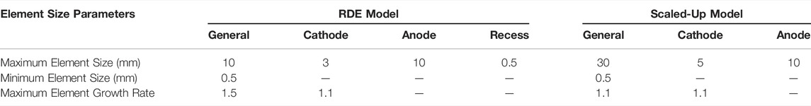
TABLE 2. User-defined, general and boundary element size parameters for both the RDE and scaled- up models.

A change only by $-50\%$ was investigated for the scaled-up model due to limitations related to the computational power of the PC hardware we use; meshes finer than $50\%$ than the control mesh exceeded the computational capacity of the hardware. The results, in terms of changes in the thickness profiles for these cases are presented in Figures 5, 6.

FIGURE 5

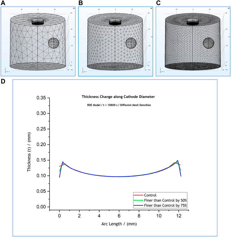
FIGURE 5. (A) Control mesh density (red), (B) mesh spacing finer than the control by 50% (green), (C) mesh spacing finer than the control by 75% (blue). Figure (D) shows an overlap of the thickness profiles predicted by the RDE model for the different mesh densities. The results simulate a 3-h process at $50 \mathit{℃}$.

FIGURE 6

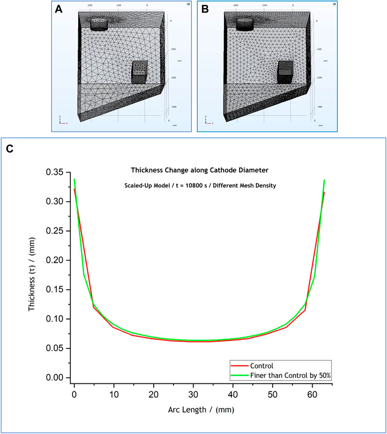
FIGURE 6. (A) Control mesh density (red), (B) mesh spacing finer than the control by 50% (green). Figure (C) shows an overlap of the thickness profiles predicted by the scaled up model for the different mesh densities. The results simulate a 3-h process at $50 \mathit{℃}$.

The local thickness profiles at the cathode boundary retrieved for $-50\%$ and $-75\%$ change in the RDE model mesh spacing and $-50\%$ change in the scaled-up model are shown in Figures 5, 6, respectively. As is expected, a finer mesh would result in smoother thickness curves since calculations are conducted at more nodes, providing solutions at more “points” throughout the electrolytic volume. However, no significant changes in the simulated thickness is observed for the RDE or the electroforming reactor, except at the outside edges where either the effect of recess or insulator is felt. On the other hand, the computation time increased significantly; from $25\text{ s}$ (Figure 5A), to $2\text{ min}$ (Figure 5B), to $36\text{ min}$ (Figure 5C) for the RDE and from $\sim 5\text{ min}$ (Figure 6A), to $\sim 36\text{ min}$ (Figure 6B) for the scaled-up system. In practice, therefore, it may be useful to optimise mesh size against computation times, especially when complicated mandrel shapes and sizes are studied.

Further still, the initial element size parameters were also changed by $\pm 5\%$, $\pm 10\%$, $\pm 12\%$, $\pm 15\%$ and $\pm 25\%$. Negative changes of these initial values mean that the mesh was made finer while positive changes led to coarser meshes.

The observations made in terms of the effect that all the above changes had on the thickness profiles are summarised in Table 3. The thickness profile graphs for the $\pm 5\%$, $\pm 10\%$, $\pm 12\%$, $\pm 15\%$ and $\pm 25\%$ are provided in the Supplementary Materials section of this publication (Supplementary Figures S6, S7). All changes are discussed in this section.

TABLE 3

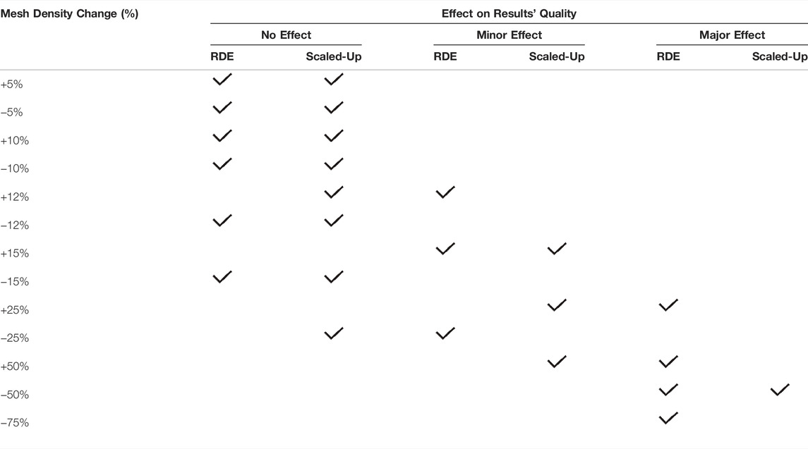
TABLE 3. Comprehensive presentation of the effect of various changes in mesh’s density on the thickness profiles for both the RDE and industrial-scale models.

Regarding the RDE model (Supplementary Figure S6), as Table 3 reveals, an increase of element size parameters by $12\%$ is the threshold after which a minor deterioration of the thickness profiles’ smoothness was observed while, major negative effect was observed following an increase by $25\%$ or more.

On the other hand, any decrease of element size parameters by up to $15\%$ did not affect the thickness profiles. Indeed, a decrease of $25\%$ was determined to be the threshold where a minor effect on the thickness profiles is observed while a decrease of $50\%$ or greater affected the profiles by showing a change in outputs where edge effects dominate. The corresponding studies for the tank system (Supplementary Figure S7), revealed a slightly different mesh tolerance. Only a decrease by $50\%$ had a major effect on the predicted thickness profile, affecting the results near the edges of the electrode, while an increase of the element size by $15\%$ and $25\%$ led to only a minor deterioration of the thickness profiles’ smoothness towards the edges.

Overall the effect on the quality of the thickness profiles retrieved and presented in Supplementary Figures S6, S7 was mainly observed at the edges. As shown in the zoomed in areas on the graphs, the thickness profiles at the middle of the deposits (arc length between $2-8\text{ mm }$ for the RDE system, and $12-48\text{ mm}$ for the tank system) are relatively undisturbed by changes in mesh spacing. Since this middle part of the deposit is used in practice, the fact that both models do not present significant mesh spacing sensitivity along that arc length is important. In industry, the area closer the edges, where the changes were observed, corresponds to the deposit part which would be discarded during post-processing to remove dendrites. Therefore, mesh-related model sensitivity may be of lower importance for electroformed products.

Geometry Sensitivity Studies

Once the models were validated, one progressed on to reactor optimisation. Geometry sensitivity studies were conducted for both the RDE, and the tank system models, investigating the effect that the anode position and cell boundaries have on the current and potential distribution. Subsequently, the observations at the two different scales were compared.

RDE System Model–Anode Position

Geometry optimisation studies were first focused on how the distance between the electrodes affects the predicted thickness profiles of the deposits. In layman’s terms this process examines when the anode placement is “felt” by the cathode (or mandrel), and at what distance this is effectively immaterial. In industry one needs to accommodate ergonomics and variation in cathode shapes, and if an arrangement was obtained when anode placement does not affect the current distribution at the cathode, then that arrangement can be used for a variety of systems.

At first, with reference to the control simulations (Figure 1A), the anode position was changed only along the z-axis, with no change along the x-axis. The anode remained off-centre at $10\text{ mm}$ from cathode same as that for the control case, whilst it was moved to 10 mm, 25 mm and $40\text{ mm}$ along the z-axis, such as shown in Figure 7. The computed results suggest that thickness profile along the RDE’s diameter (Figure 7D) does not experience any significant change. The different anode positions and their effect on the deposit thickness profile, as well as the cathode local current and potential values, are shown in Figures 7A–C. The alteration of the anode position affects the surface potential of the cathode, mainly due to the changing ohmic drop within the electrolyte; the value of ${\mathbf{\phi }}_{\mathbf{s}}$ decreases as the anode is placed further and further away.

FIGURE 7

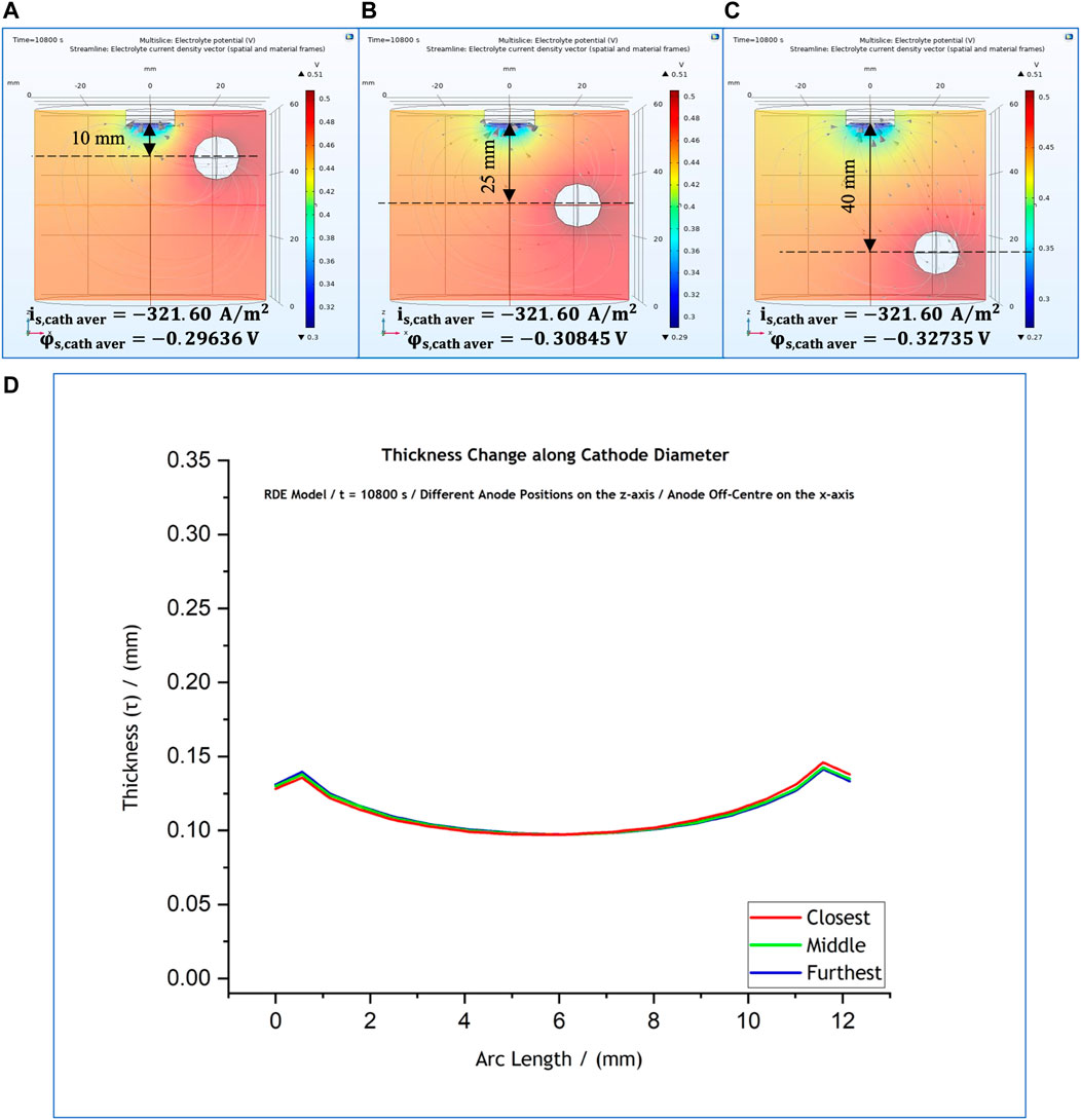
FIGURE 7. (A–C) Variations of anode position along the z-axis, with a fixed x-axis position. (D) Effect of anode position on the predicted thickness profile for anode position at 10 mm (red); 25 mm (green); and 40 mm (blue).

As a next step the anode was positioned in the centre of the cell and was varied along the z-axis, with reference to the cathode position. The position of the anode are shown in Figures 8A–C. The thickness profile (Figure 8D) again seemed to be unaffected by the movement of the anode. However, the local current density presents a notable change only when the anode is placed closest to the cathode surface, i.e., 10 cm from the cathode, when the thickness profile observed to be more flat (Figure 8D–red line) compared to the other ones corresponding to the other two anode positions.

FIGURE 8

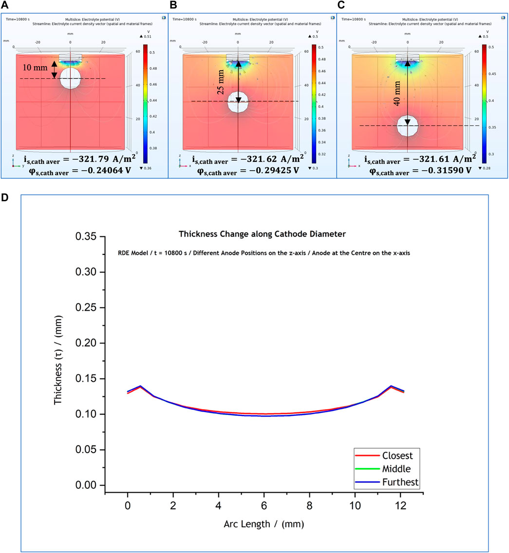
FIGURE 8. (A–C) Variations of anode position along z-axis, with a fixed x-axis position at the centre of the cell. (D) Effect of anode position on the predicted thickness profile for anode position at 10 mm (red); 25 mm (green); and 40 mm (blue).

In this regard further investigation was carried out where the anode was placed in two extreme positions: in the centre of the cell along the x-axis and at $7\text{ mm}$, the closest possible, from the cathode surface (Figures 9A,C), and off-centre at $43\text{ mm}$ from the cathode surface (Figures 9B,D). The thickness profile (Figure 9E) is differentiated from the control profile only for the anode position closest to cathode. For the position furthest from cathode the thickness profiles overlaps with the control thickness profile (and hence cannot be seen in the figure).

FIGURE 9

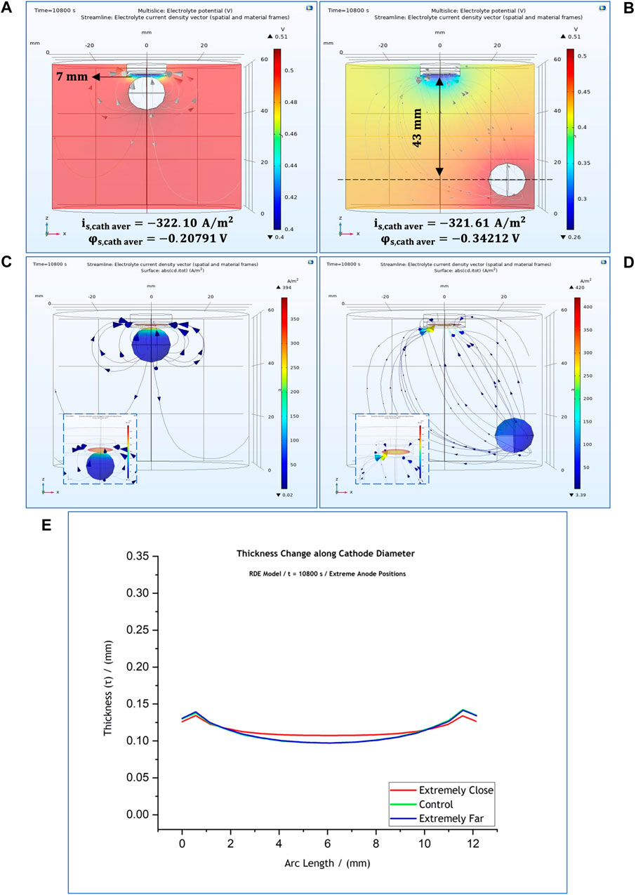
FIGURE 9. 3-D representation of the potential distribution in the electrolyte volume of the RDE model when the anode is placed at (A) $7 mm$ and (B) $43 mm$ from the cathode surface. 3-D representation of the current streamlines on the cathode surface of the RDE when the anode is placed at (C) $7 mm$ and (D) $43 mm$ from the cathode surface. (E) Thickness profiles predicted for the geometries shown in figures (A,B). The results simulate potential and current distributions after $3h$ at $50 \mathit{℃}$. Anode distances are provided with reference to its geometric centre.

This indicates that local current density presents a notable change when the anode is placed closest to cathode (Figure 9A). The local potential at the cathode surface differs due to the difference in ohmic drop with its value being $\sim 33.9\%$ higher when the anode is positioned at $7\text{ mm}$ from the cathode surface (refer to Figures 9A,B).

Our results suggest that the anode affects significantly the cathodic local potential and current density values only when it is placed closer than $10\text{ mm}$ from the cathode surface. For any greater distance between the two electrodes the anode position does not significantly affect the cathode current density value or thickness profile. In practice, it is rare for the anode vs. cathode distance to be significantly less than 10 mm. Indeed, our results indicate that it may be prudent to place it at some distance where the current distribution is less sensitive to their placement.

RDE System Model–Cell Boundaries

The next set of optimisations was focused towards determining the effect of reactor boundaries. In industry, often very large-scale systems are used, and the size of anode and cathode are changed depending on clients’ needs without any changes to tank or reactor size. It is important, therefore, to elucidate what is likely to happen to current distribution (or deposit thickness) when such arbitrary changes are made, and if engineering judgement can be applied to mitigate these changes.

For this set of studies, the electrode boundaries were kept the same as in the control simulation (with the anode placed 25 cm from the cathode surface) (Figure 3A) while the cell dimensions were doubled and potential distribution and current density at the cathode were simulated. The results of these computations are shown in Figures 10A,C. Following that, another study was carried out with the anode positioned at the bottom (48 cm from the cathode surface) (Figures 10B,D). The thickness profiles predicted for both cases are presented in Figure 10E.

FIGURE 10

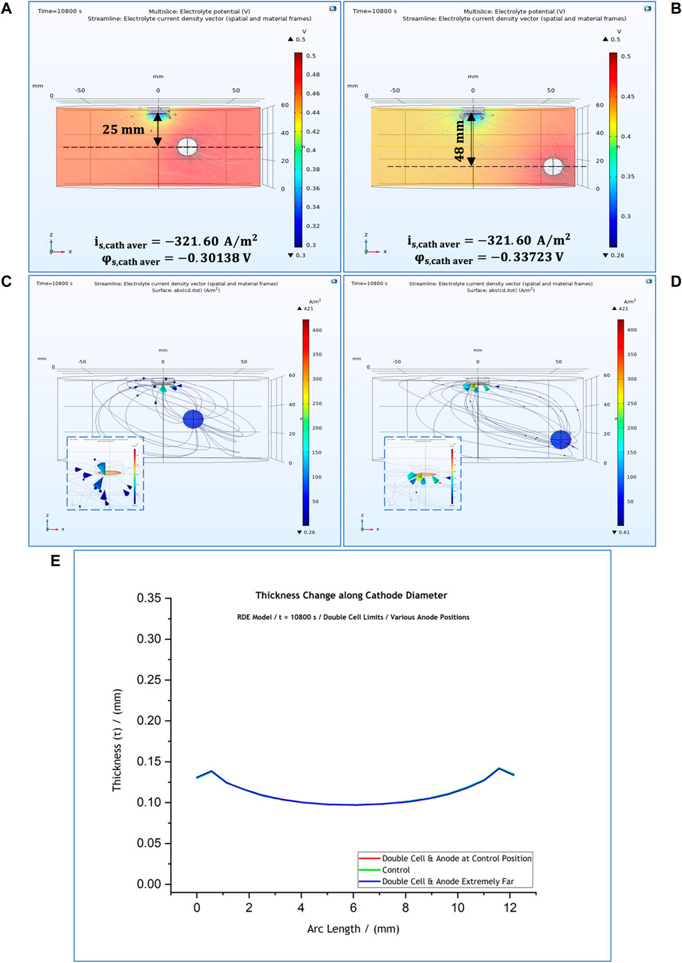
FIGURE 10. 3-D representation of the potential distribution in the electrolyte volume of the RDE model when the cell boundaries are double than the control simulations and the anode is placed off-centre, at (A) 25 mm and (B) 48 mm from the cathode surface. 3-D representation of the current distribution on the cathode surface for the two cases when the anode is placed at (C) 25 mm and (D) 48 mm from the cathode surface. (E) Thickness profiles predicted for all anode positions. The results simulate potential and current distributions after 3 h at 50°C. Distances are provided with reference to the anode’s geometric centre.

For both cases, the predicted thickness profile and local current density at the cathode remained unaffected. As it can be seen in Figures 10A,B, the cathodic local current density was calculated at $-321.60\text{ A}/{\text{m}}^2$ for both cases. Indeed, for both cases studied as part of that set of simulations, thickness profile was found to be identical as the one observed for anode distances greater than 10 mm from the cathode surface (Figure 10E). These results suggest that the size of the cell would not affect thickness distribution.

Based on our results, one can confidently suggest that, unless the distance between the electrodes is closer than 10 mm and the anode faces the cathode surface frontally, the anode position does not affect significantly the current distribution. This is important in an industrial situation, because often the placement of anode and cathode is dependent on electrode shape and size and ease of handling. Our computations show that slight changes in the position of the anode do not influence the thickness of the electroformed part, which is important in practice.

If a frontal placement of the anode, is required, additional geometry aids, like masks and thieves, might be needed to achieve the desired thickness uniformity. It is important to highlight here that exploring the effect of the anode is not of interest in this case because electroforming systems use anodes with surface areas at least double in size compared to cathode surface to avoid anode passivation (Roy and Andreou, 2020). As a result, real-life production setups render the size of the anode surface to be, somehow, irrelevant to the model design for electroforming.

Electroforming Reactor Model

The next reasonable step of this study was to investigate whether the conclusions drawn following the RDE simulations are also confirmed for the electroforming reactor. In this case too, the effect of three different anode positions on the industrial-scale system’s behaviour was investigated. These positions are shown in Figures 11A–C. Specifically, the system was studied with the anode placed at the control position, $160\text{ mm}$ from cathode (Figure 11A), at $5\text{ mm}$ below the cathode but off-centre (Figure 11B), and at $10\text{ mm}$ from cathode facing its surface frontally (Figure 11C). The off-centre and frontal positions are determined with reference to the anode’s geometric centre.

FIGURE 11

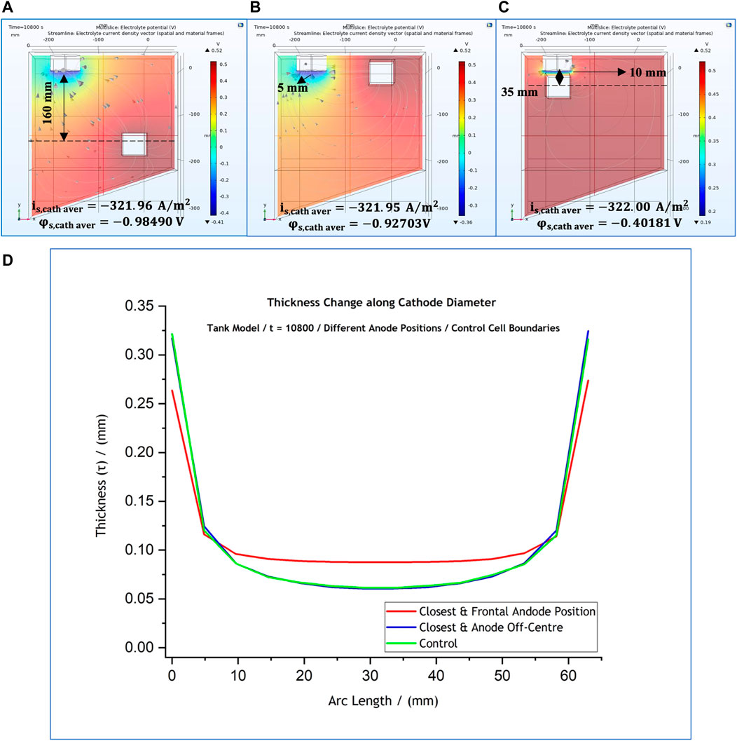
FIGURE 11. (A–C) 3-D representation of the potential distribution in the electrolyte volume of the tank system model for anode positions at different distances from the cathode surface. Current streamlines in the electrolyte are also shown. (D) Effect of anode position on the predicted thickness profile. The local cathodic potential and current density values are provided for each case. The results simulate potential and current distributions after 3 h at 50°C. Distances are provided with reference to the anode’s geometric centre.

The effect of each one of the anode positions on the thickness profile, as well as the cathodic local current and potential values for each case, are shown in Figure 11. The computed results suggest that thickness profile along the mandrel’s diameter (Figure 11D) is the same for the two cases when the cathode is off-centre; a more uniform thickness (hence current density) for the central part of the cathode is observed only for part (c). The alteration of the anode position has an effect on the local potential due to changes in ohmic drop within the electrolyte. These results are very similar to the findings for the RDE simulations discussed earlier.

The alteration of the anode position has an effect on the local potential, but the local current density on the cathode surface remained unaffected. Local current density was calculated at $-322\text{ A}/{\text{m}}^2$ for all anode positions. These results are in total agreement with the ones expected following the RDE simulations discussed earlier.

Studies on the effect of anode position where the dimensions of the cell were doubled (36 L) were also conducted (Figures 12A–C). Three different anode positions were examined; these varied among the frontal anode position at 10 mm from cathode and two other anode positions, as shown in Figures 12A-C. For all three cases the predicted thickness profile is presented in Figure 12D. Once more, the current distribution at the mandrel is identical for the cases when the anode is placed further away, and becomes more uniform over the central part of the mandrel when the anode is placed frontally at $10\text{ mm}$ from the cathode surface.

FIGURE 12

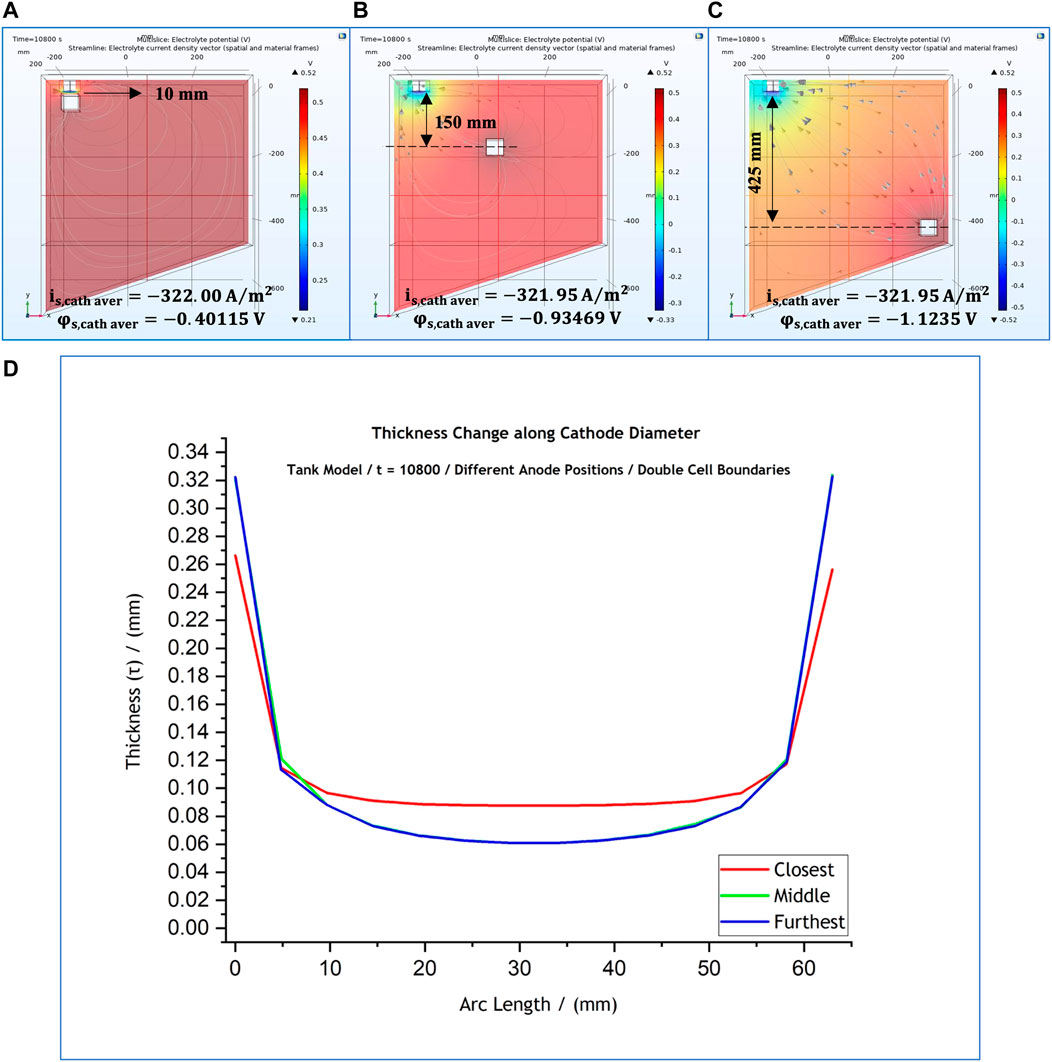
FIGURE 12. (A–C) 3-D representation of the potential distribution in the electrolyte volume of the tank system model for anode positions at different distances from the cathode surface when cell boundaries are doubled. Current streamlines in the electrolyte are also shown. (D) Effect of anode position on the predicted thickness profile. The local cathodic potential and current density values are provided for each case. The results simulate potential and current distributions after 3 h at 50°C. Distances are provided with reference to the anode’s geometric centre.

Conclusion

Nickel electroforming, time-dependent, models of two different scales were developed using a commercial software and were successfully validated against experimental data. The models were based on the assumptions of secondary current distribution (SCD) using Butler-Volmer kinetics. One model was developed to simulate the nickel electroforming process in a laboratory using a rotating disk electrode (RDE) while the second one represented an industrial, $18\text{L}$, electroforming reactor configuration.

Electrochemical experimental data, collected via polarisation studies were used as input for both models. The reaction at the cathode and anode were based on the overall nickel reduction and dissolution reactions, respectively. Current-potential data was used to fit exchange current density and forward and backward charge transfer coefficients. From the experimental measurements the equilibrium potential was found to be −0.52 V. The model could be used to predict current-potential data even though a detailed reaction mechanism was not used.

At first, a set of control simulations, modelling deposition processes, in both scales, at current values similar with those applied by the industry, were carried out to determine the potential and current at the electrode surface. The simulated results suggested that he total current and anode potential remain fixed, while the cathode surface local potential is adjusted by the model to calculate the local current density, which is then summed up to obtain the total current density, and compared against the value set for the simulation.

The results obtained were validated by cross-checking the thickness of an electroformed disk using the RDE as well as the electroforming reactor. It was found that the formed material on the RDE was thinner than the predicted value. The thickness of the disk formed within the electroforming reactor, on the other hand, agreed reasonably with the values computed by the model. The difference in the agreement between the calculated and experimental value for the RDE was attributed to the growth of dendrites along the circumferential edge of the disk.

Mesh sensitivity studies were conducted to determine both models’ inherent mesh spacing tolerance, as well as any differences observed between the two scales. Developed meshes for both models presented with a similar high element quality at $\sim 0.65$. The control meshes of both models were modified by $\pm 5\%$, $\pm 10\%$, $\pm 12\%$, $\pm 15\%$, $\pm 25\%$, $\pm 50\%$ and $-75\%$. Regarding the RDE model, an increase of mesh element size by $12\%$ and a decrease of $25\%$ were found to be the thresholds after which a minor deterioration of the thickness profiles’ smoothness was observed. For the electroforming reactor model, the corresponding results revealed that an increase of the element size by $15\%$ and a decrease by $50\%$ had a major effect on the predicted thickness profiles’ smoothness. However, no significant changes in the simulated thickness were observed for either model, while the computation time increased significantly for the finest meshes in both scales. Therefore, in practice, it is suggested that mesh spacing should be optimised against computation times.

Studies on the effect of anode location, which dictated the anode-cathode distance, on current uniformity within the RDE or reactor were performed using the models. It was found that anode positioning did not play a major role on the uniformity of the deposit. Secondly, the geometry of the reactor was changed to determine the effect of reactor boundaries on current uniformity.

For both scales, placing the anode frontally to the cathode, and within $10\text{ mm}$ of the deposition surface, resulted in increased thickness uniformity all over the electroform’s “useful” area. Outside the $10\text{ mm}$ proximity zone, the models suggested that changes in anode position increase the ohmic potential drop, but stop affecting current distribution. These results are relevant to industrial situations, because one would like to minimise changes to the electroforming process due to anode positioning or reactor geometry.

Data Availability Statement

The original contributions presented in the study are included in the article/Supplementary Material, further inquiries can be directed to the corresponding author.

Author Contributions

EA designed the research, performed the practical experiments and developed the models. EA drafted the manuscript. SR revised the manuscript. SR supervised the project. All authors contributed to the article and approved the submitted version.

Funding

This work was financially supported by the Scottish Research Partnership in Engineering (SRPe) under the National Manufacturing Institute Scotland Industry Doctorate Programme (NMIS-IDP) and Radius Aerospace—Bramah.

Conflict of Interest

The authors declare that the research was conducted in the absence of any commercial or financial relationships that could be construed as a potential conflict of interest.

Publisher’s Note

All claims expressed in this article are solely those of the authors and do not necessarily represent those of their affiliated organizations, or those of the publisher, the editors and the reviewers. Any product that may be evaluated in this article, or claim that may be made by its manufacturer, is not guaranteed or endorsed by the publisher.

Acknowledgments

The authors would like to thank Michael Watt (University of Strathclyde) for constructing the scaled-up, 18L, electroforming reactor used for validation experiments. They would also like thank James Kelly (University of Strathclyde) for his assistance with deposit preparation for thickness measurements (sectioning and mounting).

Supplementary Material

The Supplementary Material for this article can be found online at: https://www.frontiersin.org/articles/10.3389/fceng.2022.755725/full#supplementary-material

Supplementary Figure S1 | In scale (1:1) schematic of the RDE setup. The cathode was a recessed system, providing more uniform current density as compared to a RDE without a recess.

Supplementary Figure S2 | In scale (1:3) top- and side-view schematic of the tank’s interior including equipment.

Supplementary Figure S3 | Sectioning of nickel disk deposits formed (A) in the tank system and (B) in the RDE system for thickness measurements. The white arrows indicate the side face of its section measured under the microscope, following these being mounted in a (C) resin specimen.

Supplementary Figure S4 | Real-life nickel electroforms produced in the laboratory-scale RDE setup. The deposit was formed at −5 V and −0.565 A, for 1800 s. The experiment was conducted at 50°C, under agitation.

Supplementary Figure S5 | Real-life nickel electroforms produced in the prototype electroforming reactor. The deposit was formed at −2.5 V and −1 A, for 10,800 s. The experiment was conducted at 50°C, under agitation.

Supplementary Figure S6 | Overlap of thickness profiles predicted by the RDE model following (A) an increase of the element size parameters by various percentages and (B) a decrease of the element size parameters by various percentages. Figure (A) shows the change in the results’ quality for meshes coarser than the control mesh while, figure (B) shows the change in the results’ quality for meshes finer than the control mesh. The results simulate a 3-h process at $50$°C.

Supplementary Figure S7 | Overlap of thickness profiles predicted by the scaled-up model following (A) an increase of the element size parameters by various percentages and (B) a decrease of the element size parameters by various percentages. Figure (A) shows the change in the results’ quality for meshes coarser than the control mesh while, figure (B) shows the change in the results’ quality for meshes finer than the control mesh. The results simulate a 3-h process at $50$°C.

Supplementary Table S1 | Model physical and (electro) chemical input parameters.

Supplementary Table S2 | User-defined, general and boundary, user-defined, element size parameters for both the RDE and scaled-up models.

Supplementary Table S3 | Comprehensive presentation of the effect of various changes in mesh’s density on the thickness profiles modelled for both the RDE and industrial-scale models.

Abbreviations

$\mathbf{A}$, surface of deposited area; ${\mathbf{E}}_{\mathbf{eq},\mathbf{m}}$, equilibrium potential of a reaction $\text{m}$; $\mathbf{F}$, Faraday’s constant; ${\mathbf{I}}_{\mathbf{l},\mathbf{total}}$, input (applied) electrolyte current; ${\mathbf{i}}_{\mathbf{loc}}$, local current densities in the electrolyte close to electrode; ${\mathbf{i}}_{\mathbf{s},\mathbf{cath} \mathbf{aver}}$, average local cathode surface current density; ${\mathbf{i}}_{\mathbf{s}}$, local current density at the electrode surface; ${\mathbf{i}}_{0,\mathbf{m}}$, exchange current density of a reaction $\text{m}$; ${\mathbf{i}}_{\mathbf{loc},\mathbf{m}}$, local charge transfer current density of a reaction $\text{m}$; $\mathbf{M}{\mathbf{r}}_{\mathbf{Ni}}$, dissolving-depositing species molar weight, molar weight of nickel; ${\mathbf{\eta }}_{\mathbf{m}}$, activation overpotential; $\mathbf{\sigma }$, electrolyte conductivity; $\mathbf{phis}$, electric (electrode) potential; $\mathbf{phil}$, electrolyte potential${\mathbf{\rho }}_{\mathbf{Ni}}$, dissolving-depositing species density, density of nickel; $\mathbf{R}$, universal gas constant; $\mathbf{T}$, electrolyte temperature; ${\mathbf{\alpha }}_{\mathbf{c},\mathbf{m}}$, cathodic charge transfer coefficient of a reaction $\text{m}$; ${\mathbf{\alpha }}_{\mathbf{a},\mathbf{m}}$, anodic charge transfer coefficient of a reaction $\text{m}$; ${\mathbf{\phi }}_{\mathbf{s},\mathbf{cath} \mathbf{aver}}$, average local cathode surface potential; ${\mathbf{\phi }}_{\mathbf{s},\mathbf{ext},\mathbf{init}}$input electrode potential; ${\mathbf{\phi }}_{\mathbf{s}}$, local potential at the electrode; ${\mathbf{\phi }}_{\mathbf{l}}$, local potential in the electrolyte; $\mathbf{\phi }$, local potential; $\nabla =\mathit{i}\frac{\mathit{d}}{\mathit{dx}}+\mathit{j}\frac{\mathit{d}}{\mathit{dy}}+\mathit{k}\frac{\mathit{d}}{\mathit{dz}}$, Nabla, differential operator.

References

Andreou, E., and Roy, S. (2021). Modelling the Electroforming Process: Significance and Challenges. Transactions of the IMF 99 (6), 299–305. doi:10.1080/00202967.2021.1956813

CrossRef Full Text | Google Scholar

ARCHIE-WeSt (2021). Research Computing for the West of Scotland. University of Strathclyde. Available: https://www.archie-west.ac.uk/ (Accessed August 02, 2021).

Google Scholar

Baudrand, D. (1996). Nickel Sulfamate Plating, its Mystique and Practicality. Metal Finishing 94, 15–18. doi:10.1016/0026-0576(96)81353-5

CrossRef Full Text | Google Scholar

Behagh, A., Tehrani, A. F., Jazi, H. S., and Behagh, O. (2015). Simulation of Nickel Electroforming Process of a Revolving Part Using Finite Element Method. Iranian J. Mater. Sci. Eng. 12 (1), 20–27.

Google Scholar

Belov, I., Zanella, C., Edström, C., and Leisner, P. (2016). Finite Element Modeling of Silver Electrodeposition for Evaluation of Thickness Distribution on Complex Geometries. Mater. Des. 90, 693–703. doi:10.1016/j.matdes.2015.11.005

CrossRef Full Text | Google Scholar

Berggren, M. (2012). A Brief Introduction to the Finite Element Method. Umeå: Department of Computing Science, Umeå University.

Google Scholar

Bouzek, K, Borve, K., Lorentsen, O. A., Osmundsen, K., Rousar, I., and Thonstad, J. (1995). Current Distribution at the Electrodes in Zinc Electrowinning Cells. J. Electrochem. Soc. 142, 64–69. doi:10.1149/1.2043939

CrossRef Full Text | Google Scholar

Committee B-8 Staff (1962). Symposium on Electroforming - Applications, Uses and Properties of Electroformed Metal. Philadelphia, USA: American Society for Testing Materials.

Google Scholar

Comsol (2021). Mesh Element Quality and Size. Available: https://doc.comsol.com/5.5/doc/com.comsol.help.comsol/comsol_ref_mesh.15.18.html (Accessed 01 11, 2022).

Google Scholar

Davies, D. P., and Jenkins, S. L. (2014). Mechanical and Metallurgical Characterisation of Electroformed Nickel for Helicopter Erosion Shield Applications. Mater. Sci. Eng. A 607, 341–350. doi:10.1016/j.msea.2014.03.122

CrossRef Full Text | Google Scholar

Dinan, T. E., Matlosz, M., and Landolt, D. (1991). Experimental Investigation of the Current Distribution on a Recessed Rotating Disk Electrode. J. Electrochem. Soc. 138, 2947–2951. doi:10.1149/1.2085346

CrossRef Full Text | Google Scholar

Elsyca, N. V. (2021). Elsyca. Available: https://www.elsyca.com/ (Accessed August 02, 2021).

Google Scholar

Ford, S., and Despeisse, M. (2016). Additive Manufacturing and Sustainability: an Exploratory Study of the Advantages and Challenges. J. Clean. Prod. 137, 1573–1587. doi:10.1016/j.jclepro.2016.04.150

CrossRef Full Text | Google Scholar

Grande, W. C., and Talbot, J. B. (1993). Electrodeposition of Thin Films of Nickel‐Iron: II. Modeling. J. Electrochem. Soc. 140, 675–681. doi:10.1149/1.2056141

CrossRef Full Text | Google Scholar

Henquín, E. R., and Bisang, J. M. (2009). Comparison between Primary and Secondary Current Distributions in Bipolar Electrochemical Reactors. J. Appl. Electrochem. 39, 1755–1762. doi:10.1007/s10800-009-9874-6

CrossRef Full Text | Google Scholar

Hessami, S., and Tobias, C. W. (1989). A Mathematical Model for Anomalous Codeposition of Nickel‐Iron on a Rotating Disk Electrode. J. Electrochem. Soc. 136, 3611–3616. doi:10.1149/1.2096519

CrossRef Full Text | Google Scholar

Heydari, H., Ahmadipouya, S., Maddah, A. S., and Rokhforouz, M.-R. (2020). Experimental and Mathematical Analysis of Electroformed Rotating Cone Electrode. Korean J. Chem. Eng. 37 (4), 724–729. doi:10.1007/s11814-020-0479-4

CrossRef Full Text | Google Scholar

Hindle, C. (2021). Polypropylene (PP). British Plastics Federation. Available: https://www.bpf.co.uk/plastipedia/polymers/pp.aspx#physicalproperties (Accessed 09 30, 2021).

Google Scholar

International, A. (2003). Standard Guide for Electroforming with Nickel and Copper. West Conshohocken, USA: ASTM International.

Google Scholar

Jianhua, R., Zengwei, Z., and Di, Z. (2016). Effects of Process Parameters on Mechanical Properties of Abrasive-Assisted Electroformed Nickel. Chin. J. Aeronautics 29 (4), 1096–1102.

Google Scholar

John, S., Ananth, V., and Vasudevan, T. (1999). Improving the deposit Distribution during Electroforming of Complicated Shapes. Bull. Electrochemistry 15, 202–204.

Google Scholar

Khazi, I., and Mescheder, U. (2019). Micromechanical Properties of Anomalously Electrodeposited Nanocrystalline Nickel-Cobalt Alloys: a Review. Mater. Res. Express 6, 082001. doi:10.1088/2053-1591/ab1bb0

CrossRef Full Text | Google Scholar

Krause, T., Arulnayagam, L., and Pritzker, M. (1997). Model for Nickel‐Iron Alloy Electrodeposition on a Rotating Disk Electrode. J. Electrochem. Soc. 144, 960–969. doi:10.1149/1.1837514

CrossRef Full Text | Google Scholar

Krusell, E. (2019). Best Rractices for Meshing Domains with Different Size Settings. COMSOL Multiphysics. Available: https://uk.comsol.com/blogs/best-practices-for-meshing-domains-with-different-size-settings/ (Accessed August 02, 2021).

Google Scholar

Kume, T., Egawa, S., Mimura, G., and Mimuraa, H. (2016). Influence of Residual Stress of Electrodeposited Layer on Shape Replication Accuracy in Ni Electroforming. Proced. CIRP 42, 783–787. doi:10.1016/j.procir.2016.02.319

CrossRef Full Text | Google Scholar

Li, A., Tang, X., Zhu, Z., and Liu, Y. (2019). Basic Research on Electroforming of Fe-Ni Shell with Low thermal Expansion. Int. J. Adv. Manuf. Technol. 101, 3055–3064. doi:10.1007/s00170-018-3073-8

CrossRef Full Text | Google Scholar

Low, C. T. J., Roberts, E. P. L., and Walsh, F. C. (2007). Numerical Simulation of the Current, Potential and Concentration Distributions along the Cathode of a Rotating cylinder Hull Cell. Electrochimica Acta 52, 3831–3840. doi:10.1016/j.electacta.2006.10.056

CrossRef Full Text | Google Scholar

Madore, C., Matlosz, M., and Landolt, D. (1992). Experimental Investigation of the Primary and Secondary Current Distribution in a Rotating cylinder Hull Cell. J. Appl. Electrochem. 22, 1155–1160. doi:10.1007/bf01297417

CrossRef Full Text | Google Scholar

Madore, C., West, A. C., Matlosz, M., and Landolt, D. (1992). Design Considerations for a Cylindrical Hull Cell with Forced Convection. Electrochimica Acta 37 (1), 69–74. doi:10.1016/0013-4686(92)80013-c

CrossRef Full Text | Google Scholar

Mahapatro, A., and Suggu, S. K. (2018). Modelling and Simulation of Electrodeposition: Effect of Electrolyte Current Density and Conductivity on Electroplating Thickness. Adv. Mater. Sci. 3 (2), 1–9. doi:10.15761/ams.1000143

CrossRef Full Text | Google Scholar

Matlosz, M. (1993). Competitive Adsorption Effects in the Electrodeposition of Iron‐Nickel Alloys. J. Electrochem. Soc. 140, 2272–2279. doi:10.1149/1.2220807

CrossRef Full Text | Google Scholar

Matlosz, M., Creton, C., Clerc, C., and Landolt, D. (1987). Secondary Current Distribution in a Hull Cell: Boundary Element and Finite Element Simulation and Experimental Verification. J. Electrochem. Soc. 134, 3015–3021. doi:10.1149/1.2100332

CrossRef Full Text | Google Scholar

Müller, J., Buliga, O., and Voigt, K. (2018). Fortune Favors the Prepared: How SMEs Approach Business Model Innovations in Industry 4.0. Technol. Forecast. Soc. Change 132, 2–17.

Google Scholar

Newman, J., and Thomas-Alyea, K. E. (2004). Electrochemical Systems. Hoboken, NJ: John Wiley & Sons, 419–458.

Google Scholar

Nouraei, S., and Roy, S. (2007). Electrochemical Process for Micropattern Transfer without Photolithography: a Modeling Analysis. J. Electrochem. Soc. 155 (2), D97.

Google Scholar

Pepper, D., and Heinrich, J. (2005). The Finite Element Method: Basic Concepts and Applications. Boca Raton: Taylor & Francis.

Google Scholar

Pérez, T., Arenas, L. F., Villalobos-Lara, D., Zhou, N., Wang, S., Walsh, F. C., et al. (2020). Simulations of Fluid Flow, Mass Transport and Current Distribution in a Parallel Plate Flow Cell during Nickel Electrodeposition. J. Electroanalytical Chem. 873, 114359.

Google Scholar

Pérez, T., and Nava, J. L. (2014). Numerical Simulation of the Primary, Secondary and Tertiary Current Distributions on the Cathode of a Rotating cylinder Electrode Cell. Influence of Using Plates and a Concentric cylinder as Counter Electrodes. J. Electroanalytical Chem. 719, 106–112.

Google Scholar

Pfaffe, M. (2014). COMSOL Blog: Which Current Distribution Interface Do I Use? COMSOL Multiphysics. Available: https://www.comsol.com/blogs/current-distribution-interface-use/ (Accessed May 19, 2021).

Google Scholar

Platform Industrie 4.0 (2012). German Federal Ministry of Economic Affairs and Energy, German Federal Ministry of Education and Research. Available: https://www.plattform-i40.de/PI40/Navigation/EN/Home/home.html (Accessed July 29, 2021).

Google Scholar

Popereka, M. (1970). Internal Stresses in Electrolytically Deposited Metals. Washington, DC: National Bureau of Standards and the National Science Foundation.

Google Scholar

Popkova, E. G., Ragulina, Y. V., and Bogoviz, A. V. (2019). Industry 4.0: Industrial Revolution of the 21st Century (Studies in Systems, Decision and Control). Springer International Publishing AG.

Google Scholar

Ramasubramanian, M., Popova, S. N., Popov, B. N., White, R. E., and Yin, K. M. (1996). Anomalous Codeposition of Fe‐Ni Alloys and Fe ‐ Ni ‐ SiO2 Composites under Potentiostatic Conditions: Experimental Study and Mathematical Model. J. Electrochem. Soc. 143, 2164–2172. doi:10.1149/1.1836976

CrossRef Full Text | Google Scholar

Rivero, E. P., Granados, P., Rivera, F. F., Cruz, M., and González, I. (2010). Mass Transfer Modeling and Simulation at a Rotating cylinder Electrode (RCE) Reactor under Turbulent Flow for Copper Recovery. Chem. Eng. Sci. 65, 3042–3049. doi:10.1016/j.ces.2010.01.030

CrossRef Full Text | Google Scholar

Romankiw, L. T. (1987). “Electrodeposition Technology, Theory and Practice,” in The Electrochemical Society Proceedings Series (NJ: Pennington).

Google Scholar

Roy, S., and Andreou, E. (2020). Electroforming in the Industry 4.0 Era. Curr. Opin. Electrochemistry 20, 108–115. doi:10.1016/j.coelec.2020.02.025

CrossRef Full Text | Google Scholar

Slusarczyk, B. (2018). Industry 4.0 : Are We Ready? Polish J. Manag. Stud. 17 (1), 232–248.

Google Scholar

Stein, B. (1996). “A Practical Guide to Understanding, Measuring and Controlling Stress in Electroformed Metals,” in AESF Electroforming Symposium (Las Vegas, NV: Springer).

Google Scholar

Tribollet, B., and Newman, J. (1983). The Modulated Flow at a Rotating Disk Electrode. J. Electrochem. Soc. 130, 2016–2026. doi:10.1149/1.2119512

CrossRef Full Text | Google Scholar

Tsuru, Y., Nomura, M., and Foulkes, F. R. (2002). Effects of Boric Acid on Hydrogen Evolution and Internal Stress in Films Deposited from a Nickel Sulfamate bath. J. Appl. Electrochemistry 32, 629–634. doi:10.1023/a:1020130205866

CrossRef Full Text | Google Scholar

Uriondo, A., Esperon-Miguez, M., and Perinpanayagam, S. (2015). The Present and Future of Additive Manufacturing in the Aerospace Sector: A Review of Important Aspects. Proc. Inst. Mech. Eng. G: J. Aerospace Eng. 229 (11), 2132–2147. doi:10.1177/0954410014568797

CrossRef Full Text | Google Scholar

Wolfgang, S. R., and Hansal, E. G. (2012). Pulse Plating. Bad Saulgau: Leuze Verlag.

Google Scholar

Ying, R. Y., Ng, P. K., Mao, Z., and White, R. E. (1988). Electrodeposition of Copper‐Nickel Alloys from Citrate Solutions on a Rotating Disk Electrode: II . Mathematical Modeling. J. Electrochem. Soc. 135, 2964–2971. doi:10.1149/1.2095470

CrossRef Full Text | Google Scholar

Zhu, D., Zhu, Z., and Qu, N. S. (2006). Abrasive Polishing Assisted Nickel Electroforming Process. Ann. CIRP 55 (1). doi:10.1016/s0007-8506(07)60396-5

CrossRef Full Text | Google Scholar

Zhu, Z.-W., Zhu, D., Qu, N.-S., Wang, K., and Yang, J.-M. (2008). Electroforming of Revolving Parts with Near-Polished Surface and Uniform Thickness. Int. J. Adv. Manufacturing Tech. 39 (11-12), 1164–1170. doi:10.1007/s00170-007-1300-9

CrossRef Full Text | Google Scholar