Predictive functional control for separation processes by liquid-liquid extraction

1 Introduction

A separation process by liquid-liquid extraction is a well-known and widespread industrial technology implemented to quantitatively recover valuable chemical elements. In the nuclear industry, such processes have been used for decades to recover uranium and plutonium from spent fuel. The principles, the model used for the PUREX process and the PAREX code are detailed in reference (CEA, 2008). The process has been streamlined to become even more compact and more efficient, with a lower environmental footprint. An increasing amount of plutonium will be reprocessed and process margins will be reduced. Disturbances will evolve more quickly and sharply, making the process become more sensitive to variation of input parameters (reactive concentrations, flow rates, etc.). Consequently, the process needs to be corrected more efficiently to keep it in good operating condition. In this context, development has been resumed in order to improve process monitoring by using available physical models within the PAREX code (steady-state and transitory simulations). These developments may be regarded as an add-on module in a digital factory concept.

Results shown in this article are only from simulation. For the sake of data confidentiality, studies with the PAREX code cannot be published and numerical parameters of the process are normalized. These simulations will be validated during further experimental tests.

1.1 The process and the regulation case

One characteristic feature for solvent extraction is to simultaneously reach satisfactory recovery rates and decontamination factors. These criteria are often closely interconnected. The extraction-scrubbing step is considered, because it is representative of these competitive targets (see Figure 1). At the extraction step, in high acidic conditions, fresh solvent is loaded with recoverable elements (uranium and plutonium) and a small amount of impurities (fission products). During the process, these undesirable elements are scrubbed in lower acidic conditions and, as a fraction of uranium and plutonium is also removed, the aqueous scrubbing flow is sent back to the extraction step. The saturation of the solvent is the key point to ensuring this step works properly. If the solvent is not sufficiently saturated, impurities are extracted. On the contrary, if the solvent is too saturated, it is not able to extract uranium and plutonium any more: a part is lost in the fission product raffinate. This saturation phenomenon of the solvent led to a strong non-linearity of the process. It should be noticed that in the extraction step conditions of the PUREX process, uranium is only present as uranium (VI): in this article, uranium and uranium (VI) is equivalent.

FIGURE 1

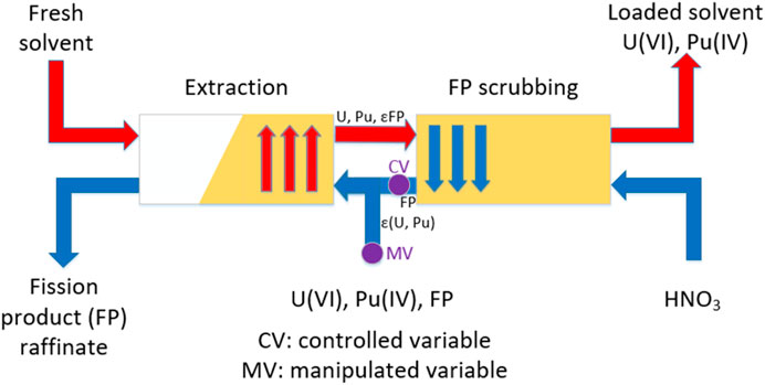
FIGURE 1. Operation principle of the extraction–fission product scrubbing step.

On the basis of sensitivity analyses, the concentration of uranium (VI) in the aqueous outflow from the scrubbing step is usually one of the best indicators to estimate this saturation. In this study, the process control aims at monitoring the solvent saturation by measuring the uranium (VI) concentration (referred to as controlled variable CV) and adjusting the feed solution flow rate (referred to as manipulated variable MV), when set point deviation occurs. The uranium (VI) concentration can be measured by spectrophotometry or estimated from density measurement.

The process regulation is studied both for set point tracking, and for disturbance rejection. The rise to the steady-state is chosen as the application case for set point tracking: monitoring is used to optimize the saturation level from zero to nominal conditions during this transient period. The objective of disturbance rejection is to keep the saturation level as close as possible to the nominal one, when disturbance occurs. Disturbances are chosen depending on two criteria. First, they have to significantly impact the saturation level of the solvent and therefore lower the recovery rates or the decontamination factors. Secondly, they need to be easily changed during experimental tests for further qualification. Fresh solvent flow rate variations fulfill these two criteria and it is why they are considered in this study as the baseline disturbance (Bisson et al., 2016). They are simulated by applying a step variation on the fresh solvent flow rate.

The higher the FP scrubbing aqueous flow rate, the more sensitive the process is. Time constants also increase with solvent saturation. In this study, simulations are carried out with two different saturation levels.

For this study, process monitoring aims at:

• Speeding up the set point tracking when the process starts up.

• Limiting CV deviations from the set point and corrects it with a quickly stabilized MV flow rate for disturbance rejection.

In both cases, upper and lower limits are applied to the MV flow rate, to keep it within a range hydrodynamically acceptable for each device.

1.2 Process special features

The process is non-linear and time constants vary over a wide range (see Figure 2). An accumulation of uranium is created due to the scrubbing step: a small amount of uranium is stripped in the aqueous phase and then reextracted at the extraction step. The size of the accumulation depends on the feed solution flow rate. Accumulation grows when the feed solution flow rate rises. This explains the increase of the time constant and the uranium (VI) concentration in the aqueous outflow on the left part of Figure 2. It takes more time for the accumulation to occur. As the accumulation grows, the uranium front moves progressively towards the raffinate outflow. From this point, a part of the uranium (VI) flows directly out in the raffinate, as the solvent becomes too saturated. When the accumulation peak is reached, the time constant decreases. The time constant is 63% of the time necessary to rise from a uranium-free process to the process at the steady-state.

FIGURE 2

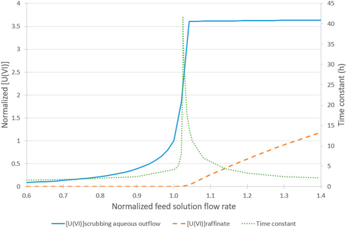
FIGURE 2. Variation of uranium (VI) concentration (left axis) and time constant (right axis) depending on normalized feed solution flow rate (the value 1.0 being the nominal flow rate).

Separation operations have been simulated by the PAREX code. Developed since the 80 s, the PAREX code has been used to design the La Hague plant flowsheets and almost all new CEA processes by solvent extraction. This code integrates physical models (reaction stoichiometry, reaction mass action law, hydrodynamics, etc.). The model is developed and qualified by checking the consistency with experimental data (batch experiments, R&D experimental pilots) on different types of contactors: mixer-settlers (Boullis and Baron, 1987) and pulsed columns (Baron and Duhamet, 1988). If necessary, the model can be extended in order to integrate new devices (like centrifugal extractor) or new species such as Neptunium (Dinh et al., 2008). The model has been extensively used to design experimental and industrial flowsheets (for instance for R4 at La Hague plant (Baron et al., 1998)). Industrial data are exploited both at the steady-state and during transient periods. This experience feedback qualifies the model in real industrial conditions at La Hague plant (Baron et al., 2008) (Dinh et al., 2013). With this significant basis, the code may be used to evaluate operating margins (Bisson et al., 2016), to design state estimator (Duterme et al., 2019a) (Duterme et al., 2019b) or diagnosis tool (Dinh et al., 2019). Simulations are performed when the process reached the steady-state, but also during transient periods, whatever set point tracking or disturbance rejection (see Figure 3). The PAREX code can be reliably used to initiate development of correctors.

FIGURE 3

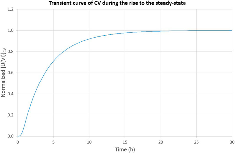
FIGURE 3. (a-top part) Transient curve of CV during the rise to the steady-state (b-bottom part) concentration profile of uranium (VI) at the steady-state.

1.3 Approach adopted

To the best of our knowledge, few studies can be found in literature about monitoring separation processes using liquid-liquid extraction. A study (Degryse, 1967) optimized the saturation level of the solvent for a plutonium purification operation in mixer-settlers. An empirical correlation between plutonium retention and the saturation level was used to estimate the state of the process. The correction was a proportional controller. The author pointed out this worked properly, but only around nominal conditions. First, the validity of the model is limited and, for instance, interactions of other species are not considered and can lead to incorrect estimates. Second, the persistent offset of the proportional controller is acceptable under limited deviations. Simulation studies were carried out on a liquid-liquid extraction column on the basis of a modal model (Bonnefoi et al., 1977). In both cases, no physical model of the process was used and regulation was operated with linear controllers.

Unpublished studies from the 90 s within the CEA concluded that process control like Proportional Integral Derivative PID was not sensitive enough to correct the PUREX process efficiently. It appears model predictive control is a promising way to address these special features. The Model Predictive Control (MPC) appears to be more efficient than classical PID controllers in most cases, and it allows the process to be monitored with smoother command. The MPC design can be applied to complex multiple-input and multiple-output MIMO systems, with process constraints taken into account (Mayne, 2014). Nevertheless, sign changes of the separation process gains are not expected, and, as it may be the most commonly used controller worldwide, PID is therefore used as a reference benchmark.

Two main control approaches are identified in literature: the direct use by command law of a physical model (Lee and Sullivan, 1988), with prior simplification or linearization, or the identification of a model specifically designed for the control purpose (for instance linear model (Ionescu et al., 2016) (Serra et al., 2017) or wave model (Lin et al., 2013) (Yao and Xinggao, 2017)). Few physical models seem to be used to monitor processes for solvent extraction. Most of the time, models are mathematically designed, such as transfer functions, or model identification. As the model already exists and has been qualified, building a metamodel would need to be checked and an extra step of development for each new process would be required. In addition, the PAREX code simulates the process sufficiently quickly, reaching an accelerating factor of several dozens with standard computers, allowing direct use without prior simplification.

In an industrial context, to keep the control scheme as simple as possible is a top criteria for an implementation. A Predictive Functional Control (PFC) control law was implemented (Richalet et al., 1987). The implementation of this law can be directly used with the existing model already implemented in the PAREX code, and a metamodel is not necessary. This algorithm can be also implemented in a programmable controller, with no major modification. It has been successfully implemented in many fields of industrial applications (Richalet, 1993) (Fulget et al., 1999) (Abdelghani-Idrissi et al., 2001) (Bouchenchir et al., 2006) (Farges et al., 2008).

This paper deals with the way how model predictive control is implemented, the modifications necessary to adapt the PFC control law to solvent extraction processes, and the simulation results on two application cases.

2 Method: command algorithm implementation with the PAREX code

Before carrying out experimental tests, a simulation tool has been developed with the PAREX code. The objectives are to simulate how the process can be regulated with the PID and PFC controllers.

2.1 PID and PFC corrector implementation

2.1.1 Principles

As shown in Figure 1, the objective is to control the aqueous concentration of uranium (VI) in the scrubbing step outlet CV by adjusting, at each sampling period T_s, the feed solution flow rate MV. For this study, delay time is considered unimportant. Figure 4 shows the simplified control structure.

FIGURE 4

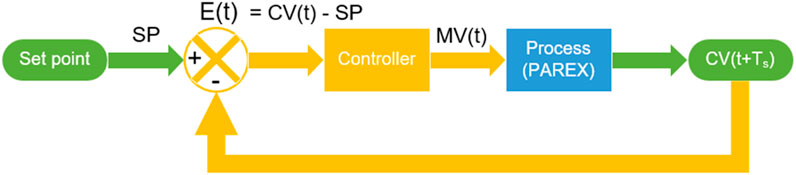
FIGURE 4. Structure of the concentration control loop with a sampling period T_s.

For the control structure, the sampling period is consistent with the residence time of phases inside an elementary cell, typically a few minutes. After each sampling, the difference between CV and set point SP is evaluated. The controller is modelled with a recursive equation with the same sampling period T_s as the process. A zero-order hold is applied to convert MV into a continuous signal: the MV signal remains constant until the next sampling period. The PAREX code simulates the process.

2.1.2 PID controller

A mixed structure is taken into account with the integral and derivative actions in parallel, and the proportional action in series (see Figure 5).

FIGURE 5

FIGURE 5. The mixed PID controller implemented.

The recursive equation of this controller with a zero-order hold is given by Equation 1:

$MV\left(k\right)=MV\left(k-1\right)+G_p\left\{\left(1+T_d\right)\epsilon \left(k\right)+\left(\frac{T_s}{T_i}-1-2.T_d\right)\epsilon \left(k-1\right)+T_d\epsilon \left(k-2\right)\right\}(1)$

2.1.3 PFC controller

The MPC controller is a well-known technique based on solving an optimization problem. Its resolution may imply a high computational cost. The PFC controller is a low-cost MPC approach avoiding complex optimization problems (Zhan et al., 2022).

Like the PID controller, the PFC controller integrates the gap between the CV concentration and the set point. However, predictive control is based on a simulation at a given time interval (Richalet et al., 1987) (see Figure 6). The correction is based on two principles. First, the model S_m is used to estimate the future behaviour of the process when applying the MV signal. Second, an exponential-type reference trajectory is defined to correct the process more or less quickly. This trajectory is fixed by only one parameter called the Closed Loop Response Time (CLRT). This parameter has to be set to find the best compromise between speed and stability. A dimensionless speed factor SF is defined as the ratio between the process time constant and the CLRT. The speed factor should be between 0.3 and 1.5. Here, the speed factor is usually 0.5.

FIGURE 6

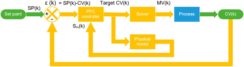
FIGURE 6. Structure of the concentration predictive control loop with a sampling period T_s.

The PFC command law is defined for a linear system at a time interval h (see Equation (2) for a first order linear system). The solvent extraction process is not linear. It is not possible to convert the target concentration into the feed solution flow rate MV with a proportional constant.

$MV\left(k\right)=\frac{l_h\epsilon \left(k\right)+b_p{S}_m\left(k\right)}{K{b}_p}(2)$

With $l_h=1-e^{-\frac{3.h.T_s}{CLRT}}$ and $b_p=1-e^{-\frac{h.T_s}{\tau }}$

The PFC algorithm needs to be adapted to a non-linear gain process. The target concentration is first evaluated with Equation (2). In this equation, K is taken equal to 1, as it is not possible to convert the target concentration into MV with a constant K. This conversion is done by a numerical solver that evaluates the feed solution flow rate MV corresponding to this target concentration, considered as a concentration at the steady state. This MV estimation is initialized with an abacus and then solves with a Newton method calling the PAREX code.

For this controller, the PAREX code is used twice, first to simulate the process as a virtual plant (CV), and then for the prediction part of the PFC command law (S_m). These are two independent calculations. For instance, the occurrence of a disturbance (or a mismatch between experimental data and model) is taken into account only for the CV calculation, not for S_m.

2.2 Comparison protocol between PID and PFC controllers

Standard methods for PID parametrization (Ziegler-Nichols, Chien-Hrones-Reswick, Cohen-Coon) were designed mostly to be applied to linear processes and were not adapted to non-linear separation processes. Without a standard parametrization for this process, it appears difficult to compare performances between the two controllers on a rigorous baseline.

As the parametrization between the two methods is different, a standard for comparison has to be defined. With accurate correction assumed to be acquired, the robustness of the controllers is studied by evaluating the stability margins.

For linear systems, the stability can be evaluated by using the gain margin in the Bode or Nyquist diagrams. Most of the time, the transfer functions should be known in order to apply this methodology. To preserve the direct use of the physical model with no intermediate metamodel, it is not envisaged to determine the transfer functions of the process. The idea is to work with the initial definition of the gain margin. This should be less than 6 dB to guarantee a sufficient margin of stability:

20.log | C (jw) · P (jw) | <6 dB (C for the controller, P for the process).

The module | C (jw) P (jw) | is a function of the controller and process gains, respectively G_C and G_P. Ensuring a gain margin of 6 dB is equivalent to doubling the controller or the process gains. Applying this factor to the controller is simple to implement in the code. Then, the response of the process is simulated to check the stability of the process.

To compare the two correctors, the protocol is as follows:

• The PID parameters are adjusted to obtain an equivalent overrun and response time (time to reach set point +/− 5%) of the two correctors during a disturbance rejection.

• Multiplying or dividing by two the gain of the corrector and simulation of the closed loop response.

The CV and MV signals are compared to determine the most robust corrector with the easiest parametrization, including the fact that few changes of the constants are necessary to make the corrector operate over a wide range of operational conditions.

3 Simulation results with a medium-level saturated solvent

3.1 Disturbance rejection

3.1.1 Simulation with the initial PFC command algorithm

The simulation starts from the nominal steady-state regime. The sampling period is 0.05 h. For the PFC controller, the time constant is determined at 14,000 s and the CLRT parameter is chosen at twice this time constant. At 0.1 h, a 5% deviation is simulated on the fresh solvent flow rate.

The PFC controller corrects the process only in the case of a −5% disturbance from the nominal fresh solvent flow rate. A persistent offset is observed for a +5% disturbance (see Figure 7). The model simulation does not take into account the disturbance effect, supposed to be unknown (Kufoalor et al., 2016). The MV signal evaluated is applied to both simulations, the model and the process. As a consequence, the model simulation point shifts towards the left part of Figure 1 for the −5% deviation (the nearly linear part) and, on the contrary, towards the right for the +5% deviation (the non-linear part). In the case of nearly linear systems, no offset is observed when rejecting a disturbance. The process incremental monitoring works because the process increment is kept proportional to model increment. For non-linear separation processes, model and process correction variations can be widely different.

FIGURE 7

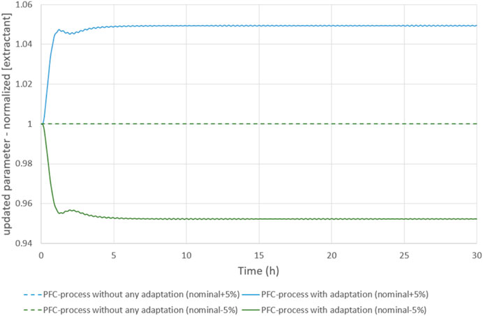
FIGURE 7. evolution of the extractant concentration to correct the model-process mismatch during a disturbance on the solvent flow rate.

Here, as a result of the +5% disturbance, the gap between the process and the model becomes too wide for the model to still be representative of the process.

This persistent offset is unusual for a PFC controller. The PFC command law takes into account the process time constant. This is responsible for an integral effect on the process monitoring, ensuring an accurate correction and the rejection of disturbances. When tracking a set point (and consequently with no significant process-model mismatch), this offset is unobserved. However, such a persistent offset was reported in (Zabet et al., 2013) (Andrade Neto et al., 2016) (Lu et al., 2018) (Wu, 2015) (Liu and Li, 2012), and identified as a consequence of unmeasured disturbances and modelling errors. A parameter estimation step was developed to better align the model with the process (Zabet et al., 2013) (Andrade Neto et al., 2016).

This persisting offset is unacceptable. This deviation cannot be removed just by adjusting the parameters of the model (time constant, CLRT). An online alignment of the model has been developed in order to improve the PFC controller.

The principle is to update the model by varying the extractant concentration, in order to cancel out the difference between the model and the process as much as possible. A 10⁻³ gap is targeted for this simulation (the CV signal does not need any filtration). This algorithm is applied as soon as a difference appears for a sampling period. This model-process mismatch correction does not aim at diagnosing the process, but at keeping the model representative of the process behaviour. The adjustment parameter is selected to be globally representative of predictable disturbances. For a separation process by liquid-liquid extraction, the extractant concentration appears to be the best candidate for the algorithm. Most disturbances at the extraction step can be modelled as a variation of the extractant concentration (Bisson et al., 2016). Nevertheless, during the transient period, this parameter does not accurately represent the evolution of each disturbance. This can generate oscillations in the target concentration and in the MV signal. To avoid this, the extractant concentration and the MV signal must be filtered (low-pass filter).

With this update of the extractant concentration (see Figure 7), the correction of the process by the PFC controller is improved for +/− 5% disturbances (see Figure 8). The PFC controller reacts to correct the process with no offset. This attests to the feasibility of accurate process monitoring when using a PFC controller.

FIGURE 8

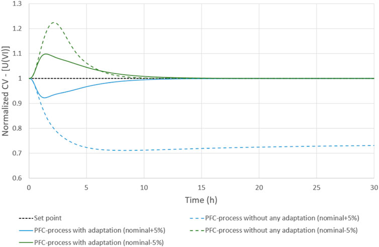
FIGURE 8. simulation of disturbance rejections with the adapted PFC command algorithm.

3.1.2 Fresh solvent flow rate disturbance +/− 15%

The simulation starts from the nominal steady-state regime. The sampling period is still 0.05 h. At 0.1 h, a +/− 15% deviation is simulated on the fresh solvent flow rate. This scenario is repeated two times: with a PID controller, and with a PFC controller. The controller constants are given in Table 1.

TABLE 1

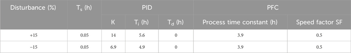
TABLE 1. Controller constants for a medium-level saturated solvent.

Both controllers manage to reach the set point. For similar performances (overrun and 95% time), the PFC controller is more stable, with no parameter change needed (see Figure 9). Through the model, the MV signal to reach the set point is more quickly determined and avoid the process oscillating. Although the variation of the fresh solvent flow rate is the same (15%), the corrections are not symmetrical, due to the difference of the process constant times.

FIGURE 9

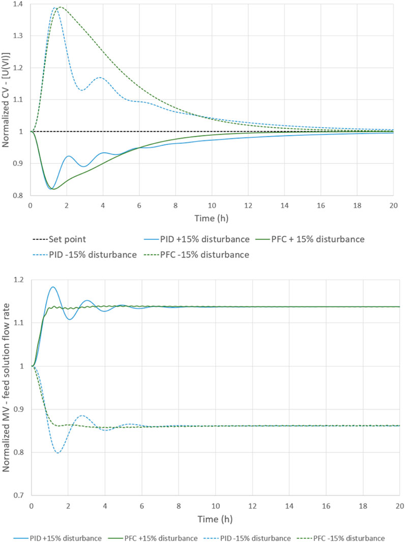
FIGURE 9. correction of a +/− 15% disturbance on the fresh solvent flow rate with PID and PFC controllers (top: CV signal, bottom: MV signal).

To further compare the two controllers, the approach described in paragraph 2.3 is applied (see Figure 10). It appears that the PFC controller has wider stability margins for the two disturbances, although the PID controller constants are manually adapted for each disturbance. When the gain was doubled, the PID controller began to oscillate. A decrease of constant times helps dampened the oscillations and avoided instability. The PFC controller can reject a wider range of disturbances, with parameters remaining unchanged and with smoother changes of the MV signal.

FIGURE 10

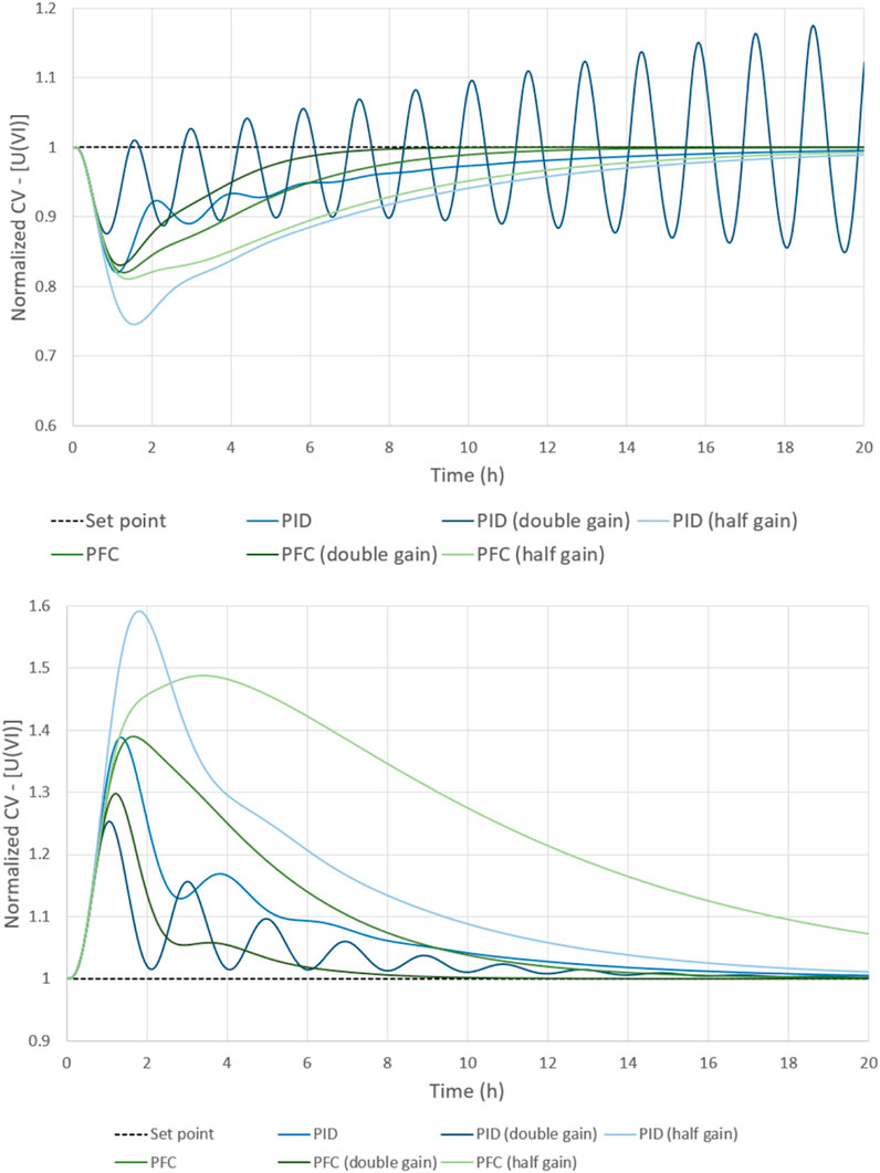
FIGURE 10. PID and PFC controller comparisons through stability margins (top: +15% disturbance, bottom: −15% disturbance).

It should be noted that the PID controller is much more sensitive to the sampling period than the PFC controller. As the sampling period increased, the process becomes less stable, with the appearance of dampened oscillations.

3.2 Set point tracking

The simulation starts with a uranium-free process flow. At the initial time (t = 0 h), the process is fed with a solution containing uranium (VI). At t = 40 h, the set point is changed from 1 to around 0.8. This scenario is repeated four times: without any controller, with a PID controller (2 sets of constants), and with a PFC controller. The sampling period is still 0.05 h. The controller constants remain those given in Table 1.

The PFC controller proves to be useful to speed up the starting procedure (see Figure 11). When the set point is changed, the PID controller reaches the new set point a little quicker, but at the cost of damped oscillations on CV and MV signals. Despite the optimization of the PID settings, its behaviour appears here to be less efficient than the open loop. This is linked to the large saturation change of the solvent, which is far beyond its nominal operating point.

FIGURE 11

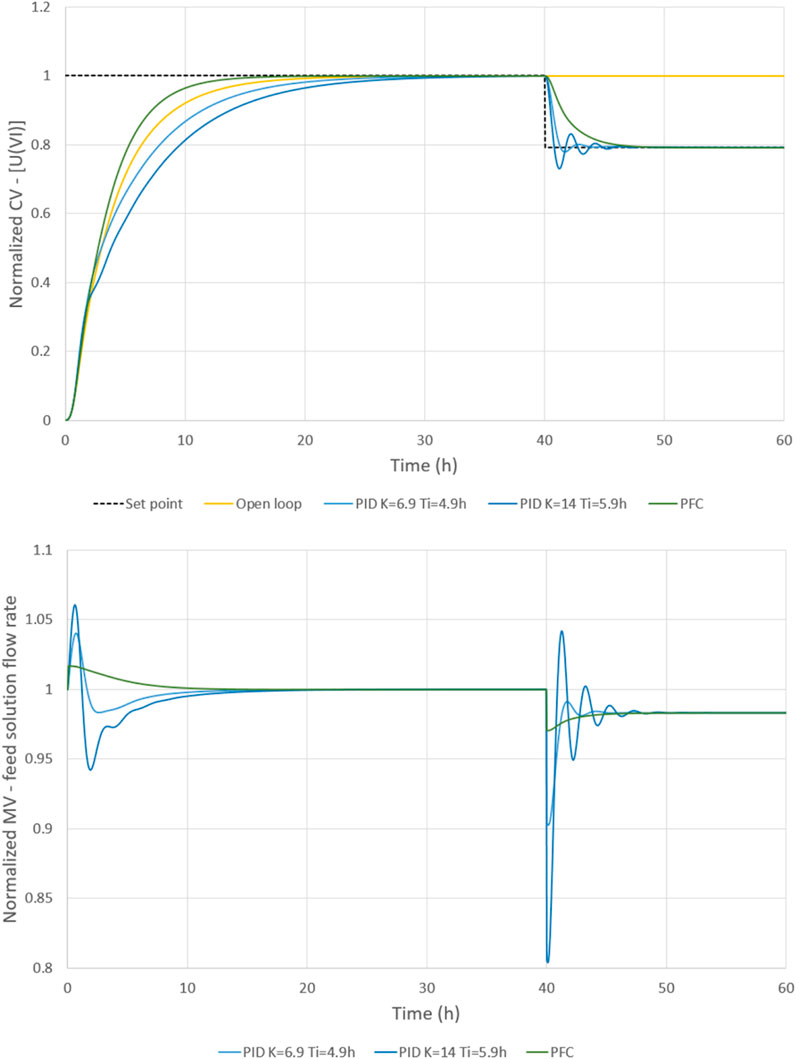
FIGURE 11. Set point tracking with PID and PFC controllers (top: CV signal, bottom: MV signal).

The absence of integral action in the predictive control enabled the process to avoid concentration overruns while reaching a zero residual difference. Once again, the PFC controller shows good performances with extended stability margins.

4 Simulation results with a high-level saturated solvent

In order to broaden the validity of the PFC control law, the second application case is to simulate a process with a more highly saturated solvent. The process is slower, with its constant time rising from 3.9 h to 12.5 h. As the model defines a slower reference trajectory, can the PFC controller still correct the process efficiently? The simulation scenarios follow the same logic as previously described.

Minimal and maximal feed solution flow rates are implemented. Here, this flow rate can vary around the nominal flow rate +/−50%. Similar limits are already fixed for the previous case, but never reached in any simulation.

4.1 Disturbance rejection

The simulation starts from the nominal steady-state regime. The sampling period is still 0.05 h. At 0.1 h, a +/− 15% deviation is simulated on the fresh solvent flow rate. This scenario is repeated two times: with a PID controller, and with a PFC controller. The controller constants are given in Table 2.

TABLE 2

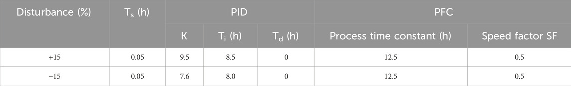
TABLE 2. Controller constants for a high-level saturated solvent.

The PFC controller manages to efficiently reject the disturbance in both cases (see Figure 12). The correction appears to be less dynamic than in the previous case, coherent with the higher time constant. The PID constants reflect this fact (higher proportional constant, lower integral constant). This explains why the stability margins are wider for both controllers (see Figure 13). The time constant does not have a sufficient impact on the PFC control law to speed up the correction. One solution tested wiss to double the correction gain, as explained in paragraph 2.3. With this small adaptation, it is feasible to correct the process more quickly, while maintaining adequate stability margins.

FIGURE 12

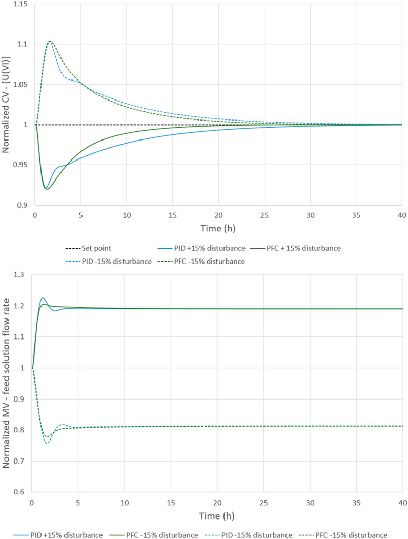
FIGURE 12. Correction of a +/− 15% disturbance on the fresh solvent flow rate with PID and PFC controllers (top: CV signal, bottom: MV signal).

FIGURE 13

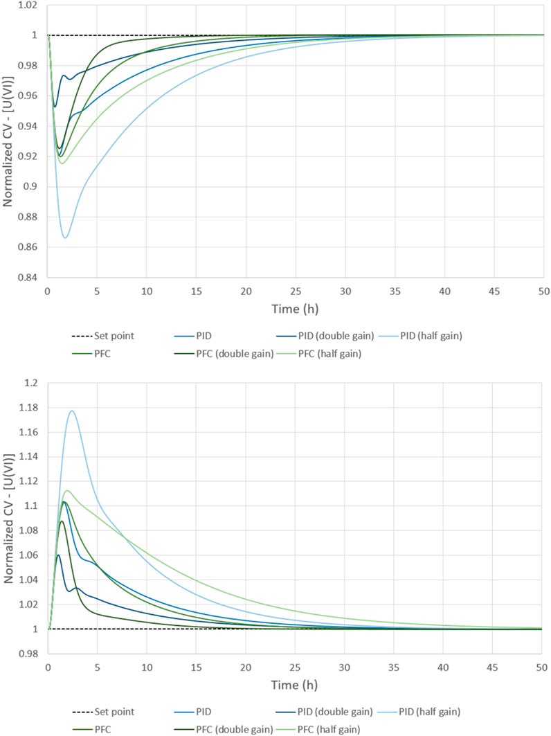
FIGURE 13. PID and PFC controller comparisons through stability margins (top: +15% disturbance, bottom: −15% disturbance).

As previously observed, the PFC controller offers more stability margins and a smoother MV signal, even if it is less marked in this case.

4.2 Set point tracking

The simulation starts with a uranium-free process flow. At the initial time (t = 0 h), the process is fed with a solution containing uranium (VI). This scenario is repeated four times: without any controller, with a PID controller (2 sets of constants), and with a PFC controller. The sampling period wis 0.05 h. The controller constants remain those given in Table 2.

The results from this starting procedure are interesting (see Figure 14). As the scrubbed uranium accumulation is bigger, more uranium is needed. The “boost” period observed during the first 1.5 h is therefore logical. The PFC controller is limited by the maximal flow rate. In that case, the variation of the MV signal is sharp at the end of the “boost” period, and it creates a transient reflux of the CV signal. The rise to the steady-state is reduced from 35.85 h (open loop) or 23.4 h (PID controller) to 17.35 h (PFC controller). This is a significant reduction, with no set point overrun in any cases. The PFC controller’s behaviour is more consistent with the standard process monitoring. When the set point is changed, the PID controller reaches the new set point more quickly. It is the same situation as for the disturbance rejection, and it is possible to improve this by adjusting the gain of the PFC control law. But the differences in the stability margins are lower for set point tracking (see Figure 14), especially for the initial rise from a uranium-free process (time from 0 h to 60 h). In fact, when the gain is greater than one, the “boost” period is too long, and the PFC controller compensates by reducing the feed solution flow rate to the minimal level. It is necessary to differentiate between a set point tracking from zero and a set point tracking from an already established steady-state. The gain can be respectively one, and two or three, to have good performances for the PFC controller.

FIGURE 14

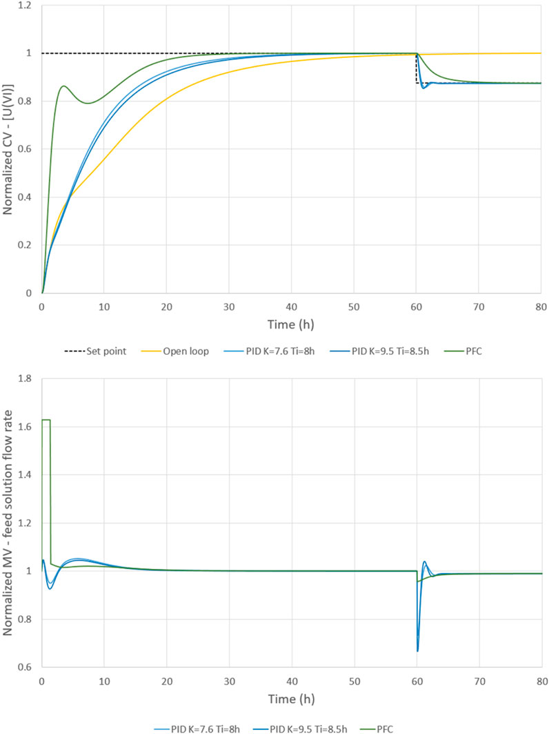
FIGURE 14. Set point tracking with PID and PFC controllers (top: CV signal, bottom: MV signal).

5 Discussion, conclusions and prospects

A simulation tool has been developed to implement the PID and Predictive Functional Control (PFC) controllers for separation processes by liquid-liquid extraction. The PFC command law manages to monitor non-linear separation processes, when using a physical model connected to the PAREX code. An online alignment of the model with the process values is necessary to keep the model sufficiently representative to predict the future behaviour of the process.

Even if the PID controller may be more efficient locally, the great strength of the PFC controller is to enable good performances on wider operating conditions, with an easier parameterization. For slow processes with the time constant process in hours, the PID parametrization would be very long to achieve because it often needs iterative adjustments. In addition, the PID controller requires to set two coefficients for the proportional and integral actions, instead of only one for the PFC controller: the speed factor. The speed factor is more intuitive for operators to handle: it has a clear physical meaning.

In the case of the PFC controller, implicitly, the physical model intervenes in the automatic settings of the parameters. The PFC controller can regulate the process with more smoothly manipulated variables, whatever the set point tracking or the disturbance rejection. In the absence of an integral action, the PFC controller has wider stability margins, enabling an increase in the correction gain to speed up the correction, especially in the case of a slow process. Such conclusions are already reported for dividing wall columns for different MPC controllers (Adrian et al., 2004) (Qian et al., 2016) (Jianxin et al., 2018).

This article shows the feasibility to regulate solvent saturation at the extraction step of the PUREX process in different conditions of saturation, with a PFC algorithm using predictions from the PAREX code, without any intermediate metamodel. Thus, the PFC controller appears to be a good candidate for experimental tests. Future experimental tests are foreseen to validate the simulation of a separation process in mixer-settlers with a surrogate feed solution. This experimental program aims at testing the PFC algorithm during different phases of operation of the process: starting procedure, nominal operation and flushing procedure. The first objective is to boost the starting procedure by rising the process to the steady-state more quickly than the current procedure (open loop in this article). Secondly, when the set point is reached, a disturbance is applied on the process to test the ability of the algorithm to keep the set point at its nominal value. An example of disturbance is a decrease of the solvent flow rate. The final objective is to speed up the uranium flushing of the process.

A mid-term objective is to include the state estimator tool in the control loop in order to consolidate the controlled variable measurements (Duterme et al., 2019a) (Duterme et al., 2019b) (Hovd and Bitmead, 2005) (MengLing et al., 2015).

Data availability statement

The original contributions presented in the study are included in the article/Supplementary materials, further inquiries can be directed to the corresponding author.

Author contributions

VV: Conceptualization, Methodology, Writing–original draft. JM: Conceptualization, Methodology, Writing–original draft. BD: Methodology, Validation, Writing–review and editing. SM: Methodology, Validation, Writing–review and editing. MM: Methodology, Validation, Writing–review and editing. FV: Methodology, Validation, Writing–review and editing.

Funding

The author(s) declare that no financial support was received for the research, authorship, and/or publication of this article.

Conflict of interest

The authors declare that the research was conducted in the absence of any commercial or financial relationships that could be construed as a potential conflict of interest.

Publisher’s note

All claims expressed in this article are solely those of the authors and do not necessarily represent those of their affiliated organizations, or those of the publisher, the editors and the reviewers. Any product that may be evaluated in this article, or claim that may be made by its manufacturer, is not guaranteed or endorsed by the publisher.

References

Abdelghani-Idrissi, M. A., Arbaoui, M. A., Estel, L., and Richalet, J. (2001). Predictive functional control of a counter current heat exchanger using convexity property. Chem. Eng. Process. 40, 449–457. doi:10.1016/s0255-2701(00)00143-4

CrossRef Full Text | Google Scholar

Adrian, T., Schoenmakers, H., and Boll, M. (2004). Model predictive control of integrated unit operations: control of a divided wall column. Chem. Eng. Process. 43, 347–355. doi:10.1016/s0255-2701(03)00114-4

CrossRef Full Text | Google Scholar

Andrade Neto, A. S., Secchi, A. R., Souza, M. B., and Barreto, A. G. (2016). Nonlinear model predictive control applied to the separation of praziquantel in simulated moving bed chromatography. J. Chromatogr. A 1470, 42–49. doi:10.1016/j.chroma.2016.09.070

PubMed Abstract | CrossRef Full Text | Google Scholar

Baron, P., Dinh, B., Drain, F., Gillet, B., and Mauborgne, B. (1998). “Plutonium purification cycle in centrifugal extractors: comparative study of flowsheets using uranous nitrate and hydroxylamine nitrate,” in Proceeding of the Conference: RECOD 98. 5. international conference on recycling, conditioning and disposal, France, 25-28 October 1998.

Google Scholar

Baron, P., Dinh, B., Duhamet, J., Drain, F., Meze, F., and Lavenu, A. (2008). “Plutonium purification cycle in centrifugal extractors: from flowsheet design to industrial operation,” in Proceeding of the ISEC 2008 conference, Tucson, 15-19 September 2008.

Google Scholar

Baron, P., and Duhamet, J. (1988). “Simulation of Uranium/Plutonium splitting in a pulsed column in the PUREX process,” in Proceeding of the ISEC’88 conference, Moscow, 18-24 Jul 1988, 204–206.

Google Scholar

Bisson, J., Dinh, B., Huron, P., and Huel, C. (2016). PAREX, A numerical code in the service of La Hague plant operations. Procedia Chem. 21, 117–124. doi:10.1016/j.proche.2016.10.017

CrossRef Full Text | Google Scholar

Bonnefoi, P., Dergier, C., Poujol, A., Rouyer, H., and Zwingelstein, G. (1977). “Practical application of the modal control theory to a liquid-liquid extraction column,” in Proceeding of the IFAC symposium on control of distributed parameter systems, Coventry, UK, June 28th – July 1st 1977.

Google Scholar

Bouchenchir, H., Cabassud, M., and Le Lann, M. V. (2006). Predictive functional control for the temperature control of a chemical batch reactor. Comput. Chem. Eng. 30, 1141–1154. doi:10.1016/j.compchemeng.2006.02.014

CrossRef Full Text | Google Scholar

Boullis, B., and Baron, P. (1987). “Modelling of Uranium/Plutonium splitting in PUREX process,” in I.CHEM.E. SYMPOSIUM SERIES n°103 Extraction’ 87 conference, Dounreay Uk, 22-26 June 1987, 323–330.

Google Scholar

CEA (2008). Treatment and recycling of spent nuclear fuel (actinide partitioning – application to waste management). CEA monography Available at: https://www.cea.fr/english/Documents/scientific-and-economic-publications/nuclear-energy-monographs/CEA_Monograph6_Treatment-recycling-spent-nuclear-fuel_2008_GB.pdf.

Google Scholar

Degryse, M. (1967). Electronic control of a plutonium extraction battery. R 3224 CEA doctoral thesis.

Google Scholar

Dinh, B., Moisy, Ph., Baron, P., Calor, J.-N., Espinoux, D., Lorrain, B., et al. (2008). “Modified PUREX first cycle extraction for Neptunium recovery,” in Proceeding of the ISEC 2008 conference, Tucson.

Google Scholar

Dinh, B., Montuir, M., and Baron, P. (2013). “PAREX, a numerical code for process design and integration,” in Proceeding of the GLOBAL 2013 conference, Salt Lake City, September 29th – October 3rd 2013.

Google Scholar

Dinh, B., Vanel, V., Sorel, C., Duterme, A., Montuir, M., and Ferlay, G. (2019). “Process simulation tools for process control and safeguards purpose,” in Proceeding of the GLOBAL 2019 conference, Seattle, September 22-26th 2019.

Google Scholar

Duterme, A., Montuir, M., Dinh, B., Bisson, J., Gil Martin, A., Floquet, P., et al. (2019a). Estimateur d’état basé sur la réconciliation de données et un modèle de connaissance pour le pilotage intelligent de procédés – application à une unité de traitement du combustible nucléaire usé (Data-reconciliation and physical-model based state estimator for smart process control - application to a spent nuclear fuel reprocessing unit). Nantes, France: SFGP Congress.

Google Scholar

Duterme, A., Montuir, M., Dinh, B., Bisson, J., Vigier, N., Floquet, P., et al. (2019b). “New methodology for bias identification and estimation – application to nuclear fuel recycling process,” in proceedings of the 29th European Symposium on Computer Aided Process Engineering, Eindhoven, The Netherlands.

Google Scholar

Farges, B., Poughon, L., Creuly, C., Cornet, J. F., Dussap, C. G., and Lasseur, C. (2008). Dynamic aspects and controllability of the MELiSSA project: a bioregenerative system to provide life support in space. Appl. Biochem. Biotechnol. 151, 686–699. doi:10.1007/s12010-008-8292-2

PubMed Abstract | CrossRef Full Text | Google Scholar

Fulget, N., Poughon, L., Richalet, J., and Lasseur, Ch. (1999). MELISSA: global control strategy of the artificial ecosystem by using first principles models of the compartments. Adv. Space Res. 24 (3), 397–405. doi:10.1016/s0273-1177(99)00490-1

PubMed Abstract | CrossRef Full Text | Google Scholar

Hovd, M., and Bitmead, R. R. (2005). Interaction between control and estimation in nonlinear MPC. Model. Identif. control 26 (n°3), 165–174. doi:10.4173/mic.2005.3.4

CrossRef Full Text | Google Scholar

Ionescu, C. M., Muresan, C. I., Copot, D., and De Keyser, R. (2016). Constrained multivariable predictive control of a train of cryogenic 13C separation columns. IFAC-PapersOnLine 49-7, 1103–1108. doi:10.1016/j.ifacol.2016.07.350

CrossRef Full Text | Google Scholar

Jianxin, W., Na, Y., Mengqi, C., Lin, C., and Lanyi, S. (2018). Composition control and temperature inferential control of dividing wall column based on model predictive control and PI strategies. Chin. J. Chem. Eng. 26, 1087–1101. doi:10.1016/j.cjche.2017.12.005

CrossRef Full Text | Google Scholar

Kufoalor, D. K. M., Imsland, L., and Johansen, T. A. (2016). Efficient implementation of step response models for embedded Model Predictive Control. Comput. Chem. Eng. 90, 121–135. doi:10.1016/j.compchemeng.2016.04.002

CrossRef Full Text | Google Scholar

Lee, P. L., and Sullivan, G. R. (1988). Generic model control (GMC). Comput. Chem. Eng. 12 (N°6), 573–580. doi:10.1016/0098-1354(88)87006-6

CrossRef Full Text | Google Scholar

Lin, C., Xinggao, L., Yexiang, Z., and Youxian, S. (2013). Generalized generic model control of high-purity internal thermally coupled distillation column based on nonlinear wave theory. AIChe J. 59-11, 4133–4141. doi:10.1002/aic.14141

CrossRef Full Text | Google Scholar

Liu, H., and Li, S. (2012). Speed control for PMSM servo system using predictive functional control and extended state observer. IEEE Trans. Industrial Electron. 59 (Issue 2), 1171–1183. doi:10.1109/tie.2011.2162217

CrossRef Full Text | Google Scholar

Lu, K., Zhou, W., Zeng, G., and Du, W. (2018). Design of PID controller based on a self-adaptive state-space predictive functional control using extremal optimization method. J. Frankl. Inst. 355, 2197–2220. doi:10.1016/j.jfranklin.2017.12.034

CrossRef Full Text | Google Scholar

Mayne, D. Q. (2014). Model predictive control: recent developments and future promise. Automatica 50, 2967–2986. doi:10.1016/j.automatica.2014.10.128

CrossRef Full Text | Google Scholar

MengLing, W., Hongbo, S., and Wen, Y. (2015). An observer-based Model Predictive Control strategy for distributed parameter system. IFAC-PapersOnLine 48-8, 883–887.

Google Scholar

Qian, X., Jia, S., Skogestad, S., Yuan, X., and Luo, Y. (2016). Model predictive control of reactive dividing wall column for the selective hydrogenation and separation of a C3 Stream in an Ethylene Plant. Industrial Eng. Chem. Res. 55, 9738–9748. doi:10.1021/acs.iecr.6b02112

CrossRef Full Text | Google Scholar

Richalet, J. (1993). Industrial applications of model based predictive control. Automatica 29, 1251–1274. doi:10.1016/0005-1098(93)90049-y

CrossRef Full Text | Google Scholar

Richalet, J., Abu el Ata-Doss, S., Arber, C., Kuntze, H. B., Jacubash, A., and Schill, W. (1987). “Predictive functional control. Application to fast and accurate robots,”10th IFAC Congress, Munich, Germany.

CrossRef Full Text | Google Scholar

Serra, M., Ocampo-Martinez, C., Li, M., and Llorca, J. (2017). Model predictive control for ethanol steam reformers with membrane separation. Int. J. Hydrogen Energy 42, 1949–1961. doi:10.1016/j.ijhydene.2016.10.110

CrossRef Full Text | Google Scholar

Wu, S. (2015). State space predictive functional control optimization based new PID design for multivariable processes. Chemom. Intelligent Laboratory Syst. 143, 16–27. doi:10.1016/j.chemolab.2015.02.014

CrossRef Full Text | Google Scholar

Yao, F., and Xinggao, L. (2017). An advanced control of heat integrated air separation column based on simplified wave model. J. Process Control 49, 45–55. doi:10.1016/j.jprocont.2016.11.004

CrossRef Full Text | Google Scholar

Zabet, K., Haber, R., and Mocha, K. (2013). Stabilizing gain design for PFC with estimated disturbance feed-forward. Semantic scholar: Nordic Process Control Workshop, 22–23. Oulu (Finland).

Google Scholar

Zhan, Z., Xie, L., Lu, S., Rossiter, J. A., and Su, H. (2022). A low-cost pole-placement MPC algorithm for controlling complex dynamic systems. J. Process Contro 111, 106–116. doi:10.1016/j.jprocont.2022.02.001

CrossRef Full Text | Google Scholar