Causal relationship between sea surface temperature and precipitation revealed by information flow

Introduction

The atmosphere and the ocean are vital components of climate (Bjerknes, 1969; Frankignoul, 1985) and have significant impacts on all aspects of human society, including but not limited to the economy, fishery, and agriculture (Pontecorvo et al., 1980; Semenov and Porter, 1995; Christy and Scott, 2013). Since the ocean and the atmosphere are coupled with each other through numerous processes (Karnauskas, 2020), understanding their interactions is essential for predicting the future state of climate.

It is well-known that the atmosphere drives the ocean. In 1905, Ekman (1905) proposed a fundamental theory about the ocean's response to steady wind forcing. The successors developed a theory showing that the meridional mass transport is to the first order governed by the wind stress curl and the meridional derivative of the Coriolis parameter (Sverdrup, 1947; Stommel, 1948). The large-scale organization of sea surface temperature (SST) anomalies may be associated with the anomalous atmospheric circulation via surface energy fluxes and Ekman currents (Deser et al., 2010), and it is believed that the atmosphere drives SST more than vice versa for the extratropical regions (Frankignoul, 1985).

During the last few decades, there have been many studies focusing on the mechanism of how the ocean affects the atmosphere. Two major models have been proposed to explain how SST anomalies drive the low-level atmospheric flow in the tropics. While the Matsuno-Gill model assumes that anomalous deep convection induces surface winds (Matsuno, 1966; Gill, 1980), the Lindzen-Nigam model asserts that the surface wind convergence is caused by SST gradient and should be regarded as the cause of deep convection (Lindzen and Nigam, 1987). Using an atmospheric mixed layer model, Back and Bretherton (2009) obtained a similar result with the Lindzen-Nigam model in that the SST gradient causes surface wind convergence that leads to deep convection. However, the SST above a convective threshold is also necessary to sustain deep convection (Graham and Barnett, 1987). Compared to the tropical ocean, it has long been considered that extratropical oceans are driven by atmospheric forcing and oceanic effects on the atmosphere are negligible (Frankignoul, 1985). However, recent studies have shown that SST fronts influence the atmosphere through their impacts on the static stability of the atmospheric boundary layer (Nonaka and Xie, 2003), pressure fields (Minobe et al., 2008), and atmospheric baroclinicity (Nakamura et al., 2008).

The influences between the ocean and the atmosphere are not unidirectional and two-way interactions may exist. The most prominent example is known as the Bjerknes feedback, which plays a key role in the development of the El Niño/Southern Oscillation (ENSO; Bjerknes, 1969). When the easterly trade winds are relaxed, the east-west thermocline tilt and thus upwelling of subsurface cold water in the eastern equatorial Pacific is suppressed. As a result, the zonal SST gradient is reduced and the trade winds are further slackened. Another important positive feedback process is the wind-evaporation-SST (WES) feedback (Xie and Philander, 1994; Kataoka et al., 2019). Under the mean easterly trade winds over the equatorial oceans, positive SST anomalies to the north of the equator induce anomalous northward cross-equatorial winds. Due to the Coriolis force, wind anomalies are deflected to the left in the Southern Hemisphere, while to the right in the Northern Hemisphere. As a result, trade winds are enhanced to the south and latent heat loss to the atmosphere is enhanced due to increased wind speed, whereas trade winds and thus latent heat loss are reduced to the north, and the original anomalous SST gradient across the equator is strengthened. Such feedback process plays an important role in the development of the Atlantic meridional mode (Doi et al., 2009; Kataoka et al., 2019). In addition, the SST-cloud-shortwave radiation acts as either positive or negative feedback depending on the background condition (Tozuka and Oettli, 2018). Over the warm ocean, a positive SST anomaly, for example, leads to enhanced deep convection and high clouds, resulting in less shortwave radiation at the sea surface and damping of SST anomalies (Waliser et al., 1994). On the other hand, in regions with low SSTs and subsidence in the lower troposphere, a positive SST anomaly leads to less low clouds and more shortwave radiation can reach the ocean surface (Li and Philander, 1996). In this case, the positive SST anomaly is further enhanced.

In addition to the local ocean-atmosphere interactions, remote forcing also plays a vital role in the climate system. For instance, the ENSO causes positive SST anomalies in the Indian Ocean and the South China Sea through an atmospheric bridge (Klein et al., 1999; Alexander et al., 2002). Wang (2002a,b) further proposed that a warm El Niño event would weaken the Hadley cell in the Indian and Atlantic Oceans. On the other hand, SST anomalies in the Indian Ocean are shown to influence the Pacific (Watanabe and Jin, 2002; Wu et al., 2009; Xie et al., 2009; Li et al., 2017), while the Atlantic Ocean is also demonstrated to influence the Pacific (Stouffer et al., 2006; Zhang and Delworth, 2007). In addition to the atmospheric teleconnections among the tropical oceans (Wang, 2019), teleconnections from the tropical oceans to the extratropical oceans are intensively studied. A famous example is the Pacific-North American (PNA) pattern (Wallace and Gutzler, 1981). Anomalous convection in the tropical Pacific causes a Rossby wave propagation in the atmosphere, resulting in a high in the tropical North Pacific, a low in the extratropical North Pacific, a high in northwestern America, and a low over the Gulf Stream (Horel and Wallace, 1981). Besides, the tropical Pacific can also affect the mid-latitude northwestern Pacific and southeastern Pacific by the Pacific-Japan pattern (Nitta, 1986, 1987; Kosaka and Nakamura, 2010) and the Pacific-South American (PSA) pattern (Mo and Paegle, 2001), respectively.

Partly because predictability is expected to be higher in regions where the ocean with a longer memory is predominantly driving the atmosphere, many studies have been devoted to understanding of the dominant direction in ocean-atmosphere interactions (Wang et al., 2005; Kumar et al., 2013; Kohyama and Tozuka, 2016). Those studies attempted to detect the interactions between the ocean and the atmosphere by examining correlation coefficients between SST and precipitation on monthly or seasonal time-scales (Arakawa and Kitoh, 2004; Wu and Kirtman, 2007; Chen et al., 2012). Although such studies are combined with discussions of plausible physical mechanisms to help understand the causality (Kumar et al., 2013), correlation does not necessarily mean causality. In this regard, Kalnay et al. (1986) examined the driver in the local ocean-atmosphere coupling based on the phase relationship between SST and relative vorticity anomalies in the lower troposphere. If the atmosphere were driving the ocean, a cyclonic anomaly in the atmosphere is expected to induce Ekman upwelling and thus a cold SST anomaly, but if the ocean were driving the atmosphere, a positive SST anomaly is expected to induce anomalous cyclonic circulation in the overlying atmosphere. Furthermore, some recent studies relied on causality analyses. Bach et al. (2019), for example, used Granger causality to support that the ocean is mainly driving the atmosphere in the tropical regions while vice versa among the extratropical regions. Also, Silva et al. (2021) used the Granger causality to study the teleconnections between the tropical Pacific and the globe and identified the seasonal precipitation response to SST anomalies associated with ENSO events.

In this study, we use an emerging statistical method called the normalized information flow (NIF; Bai et al., 2018), to study the causality between the ocean and the atmosphere. In contrast to the Granger causality, which is an empirical measure, the information theory-based causality measure is a quantitative measure of causality that is based on rigorous formalism (Liang, 2014). This paper is organized as follows. The dataset used in this study is described in the next section. In section Methods, a brief description of the NIF is provided. Results are presented in section Results, and conclusions and discussions are given in the final section.

Data

In this study, we use SST to represent the state of the ocean and precipitation to represent the state of the atmosphere. For the precipitation data, we use the monthly data of the fifth generation European Centre for Medium-Range Weather Forecasts (ECMWF) atmospheric reanalysis (ERA5; Hersbach et al., 2020) from 1979 to 2020. For SST, we use the monthly data of Extended Reconstructed Sea Surface Temperature version 5 (ERSST V5; Huang et al., 2017) with the same time span. The original spatial resolution of the ERA5 data and ERSST V5 data are 0.25◦ × 0.25◦ and 2◦ × 2◦, respectively, and we calculate the average value to interpolate the ERA5 data to 2◦ × 2◦. The monthly average of the SST and precipitation data is subtracted to obtain anomalies.

Methods

All time causality analysis

In this study, we use information flow (IF), which quantifies the causality based on transfer entropy, to detect the causality relationship between SST and precipitation anomalies. For two time series X₁ and X₂, Liang (2014) used the maximum likelihood estimator (MLE) to derive that the IF from X₂ to X₁ can be estimated as

$\begin{array}{ll}\begin{array}{c}{\text{T}}_{2\to 1}=\frac{{\text{C}}_{11}{\text{C}}_{12}{\text{C}}_{2\text{,}d1}-{\text{C}}_{12}^2{\text{C}}_{1,d1}}{{\text{C}}_{11}^2{\text{C}}_{22}-{\text{C}}_{11}{\text{C}}_{12}^2},\end{array}& (1)\end{array}$

where C_ij represents the covariance between X_i and X_j and C_i,dj is the covariance between X_i and $\stackrel{•}{{\text{X}}_j}$. With a limit sample sequence, $\stackrel{•}{{\text{X}}_j}$ can be obtained by finite-difference:

$\begin{array}{ll}\begin{array}{c}{\stackrel{.}{\text{X}}}_{\text{j},\text{n}}=\frac{{\text{X}}_{\text{j},\text{n}+1}-{\text{X}}_{\text{j},\text{n}}}{\text{Δ}\text{t}}.\end{array}& (2)\end{array}$

If T_{2 → 1}=0, X₂ is not a cause of X₁, while T_{2 → 1}≠0 indicates that there is a causality from X₂ to X₁.

However, to compare the importance of two variables among different regions, it is necessary to find a way to normalize the IF (Liang, 2015). For the normalization, we need to go back to how we derive T_{2 → 1}. Consider a 2D dynamical system that satisfies

$\begin{array}{ll}\begin{array}{c}\frac{\text{dx}}{\text{dt}}=\text{F}\left(\text{X},\text{t}\right)+\text{B}\left(\text{X},\text{t}\right)\stackrel{.}{\text{W}},\end{array}& (3)\end{array}$

where $\text{F}=({\text{F}}_{\text{1}},{\text{F}}_{\text{2}}), \text{X}=(x_{\text{1}},x_{\text{2}})\in {ℝ}^{\text{2}}$, $\stackrel{•}{\text{W}}$ is a 2D white noise, and B(X,t) is the perturbation amplitude. Liang (2008) has given the rate of change of the marginal entropy H₁ of X₁ in a 2D system with

$\begin{array}{ll}\begin{array}{c}\begin{array}{c}\frac{\text{d}{\text{H}}_1}{\text{dt}}=-\text{E}\left({\text{F}}_1\frac{\partial \text{log}{\rho }_1}{\partial {\text{x}}_1}\right)-\frac{1}{2}\text{E}\left({\text{g}}_{11}\frac{{\partial }^2\text{log}{\rho }_1}{\partial {\text{x}}_1^2}\right),\end{array}\end{array}& (4)\end{array}$

where E(x) means the mathematical expectation of x, ρ₁ is the marginal density of X₁, and ${\text{g}}_{\text{ij}}=\sum _{\text{k}}{\text{b}}_{\text{ik}}{\text{b}}_{\text{jk}}$. Then, we can expand out the first term on the right hand side of Equation (4) as

$\begin{array}{ll}\begin{array}{c}-\text{E}\left({\text{F}}_1\frac{\partial \text{log}{\rho }_1}{\partial {\text{x}}_1}\right)=-\text{E}\left[\frac{1}{{\rho }_1}\frac{\partial \left({\text{F}}_1{\rho }_1\right)}{\partial {\text{x}}_1}-\frac{\partial {\text{F}}_1}{\partial {\text{x}}_1}\right]\\ =\text{E}\left(\frac{\partial {\text{F}}_1}{\partial {\text{x}}_1}\right)-\text{E}\left[\frac{1}{{\rho }_1}\frac{\partial \left({\text{F}}_1{\rho }_1\right)}{\partial {\text{x}}_1}\right].\end{array}& (5)\end{array}$

According to Liang (2008), in a 2D system, the information flow from X₂ to X₁ is

$\begin{array}{ll}\begin{array}{c}{\text{T}}_{2\to 1}=-\text{E}\left[\frac{1}{{\rho }_1}\frac{\partial \left({\text{F}}_1{\rho }_1\right)}{\partial {\text{x}}_1}\right]+\frac{1}{2}\text{E}\left(\frac{1}{{\rho }_1}\frac{{\partial }^2\left({\text{g}}_{11}{\rho }_1\right)}{\partial {\text{x}}_1^2}\right).\end{array}& (6)\end{array}$

By substituting Equations (6) and (5) into Equation (4), we obtain

$\begin{array}{ll}\begin{array}{c}\begin{array}{c}\frac{\text{d}{\text{H}}_1}{\text{dt}}=\text{E}\left(\frac{\partial {\text{F}}_1}{\partial {\text{x}}_1}\right)+{\text{T}}_{2\to 1}+[-\frac{1}{2}\text{E}\left(\frac{1}{{\rho }_1}\frac{{\partial }^2\left({\text{g}}_{11}{\rho }_1\right)}{\partial {\text{x}}_1^2}\right)\\ -\frac{1}{2}\text{E}\left({\text{g}}_{11}\frac{{\partial }^2\log {\rho }_1}{\partial {\text{x}}_1^2}\right)].\end{array}\end{array}& (7)\end{array}$

From Equation (7), we can find that the marginal entropy H₁ consists of 3 parts, $\text{E}(\frac{\text{∂}{\text{F}}_1}{\text{∂}{\text{X}}_1})$ is the change rate of H₁ from X₁, T_{2 → 1} is the IF from X₂ to X₁, and the rest is the influence of other stochastic parts ${\text{H}}_1^{\text{noise}}$.

For a linear predictive system,

$\begin{array}{ll}\begin{array}{c}\text{F}=\text{f}+\text{AX}+\text{B}{\text{B}}^{\text{T}},\end{array}& (8)\end{array}$

where $\text{f}={({\text{f}}_{\text{1}},{\text{f}}_{\text{2}})}^{\text{T}}$, A=(_aij)i,j=1,2, and B=(_bij)i,j=1,2. The coefficient matrices A and B are constant. Hence, these variables will follow the Gaussian distribution (Liang, 2014). Let

$\begin{array}{ll}{\rho }_1=\frac{1}{\sqrt{2\pi }{\sigma }_1}\text{exp}\left[\frac{-{({\text{x}}_1-{\mu }_1)}^2}{2{\sigma }_1^2}\right]& (9)\end{array}$

and ${\text{H}}_1^{\text{noise}}$ be

$\begin{array}{ll}\begin{array}{c}\frac{\text{d}{\text{H}}_1^{\text{noise}}}{\text{dt}}=\frac{1}{2}\frac{{\text{g}}_{11}}{{\sigma }_1^2},\end{array}& (10)\end{array}$

where ${\text{σ}}_1^2$ can be replaced by the covariance of sample C₁₁, and g₁₁ can be obtained using the MLE in Equation (8)

$\begin{array}{ll}{\text{g}}_{11}\approx \Delta \text{tE}\left[{\left({\stackrel{.}{\text{X}}}_1-{\text{f}}_1-{\text{a}}_{11}{\text{X}}_1-{\text{a}}_{12}{\text{X}}_2\right)}^2\right].& (11)\end{array}$

Here,

$\begin{array}{ll}{\text{a}}_{11}\approx \frac{{\text{C}}_{22}{\text{C}}_{1,\text{d}1}-{\text{C}}_{12}{\text{C}}_{2,\text{d}1}}{\text{detC}}& (12)\end{array}$

$\begin{array}{ll}{\text{a}}_{12}\approx \frac{-{\text{C}}_{12}{\text{C}}_{2,\text{d}1}+{\text{C}}_{11}{\text{C}}_{2,\text{d}1}}{\text{detC}}.& (13)\end{array}$

To quantify the importance of X₂ to X₁, Bai et al. (2018) proposed a modified normalization method for T_{2 → 1}. Using $\text{abs}({\text{T}}_{2\to 1})+\text{abs}(\text{d}{\text{H}}_1^{\text{noise}}/\text{dt})$ as the normalizer, T_{2 → 1} can be normalized as

$\begin{array}{ll}{\text{τ}}_{2\to 1}^{\text{B}}=\frac{\text{abs}({\text{T}}_{2\to 1})}{\text{abs}({\text{T}}_{2\to 1})+\text{abs}\left(\frac{\text{d}{\text{H}}_1^{\text{noise}}}{\text{dt}}\right)}& (14)\end{array}$

A larger ${\text{τ}}_{2\to 1}^{\text{B}}$ means that X₂ has a more remarkable IF than other stochastic parts. Therefore, we can use ${\text{τ}}_{2\to 1}^{\text{B}}$ to compare the IF between SST and precipitation anomalies over the global ocean.

Significance test

Since a real time series data would always be affected by white noise and random error, T_{2 → 1} is unlikely to be exactly equal to zero. Thus, a significance test is essential to avoid a spurious causality. For Equation (6), Liang (2014) indicated that when N is large enough, T_{2 → 1} can be viewed approximately as normally distributed around the real value with a variance of ${(\frac{{\text{C}}_{\text{12}}}{{\text{C}}_{\text{11}}})}^{\text{2}}{\widehat{\sigma }}_{\text{12}}^{\text{2}}$. Then, we denote θ = (f₁, a₁₁,a₁₂,b₁), and a Fisher information matrix NI can be obtained as

$\begin{array}{ll}\begin{array}{c}\text{N}{\text{I}}_{\text{ij}}=-{\displaystyle \sum _{\text{n}=1}^{\text{N}}\frac{{\partial }^2\text{log}\rho \left({\text{X}}_{\text{n}+1}|{\text{X}}_{\text{n}};\widehat{\theta }\right)}{\partial {\theta }_{\text{i}}\partial {\theta }_{\text{j}}}}.\end{array}& (15)\end{array}$

Since the inverse of NI is the covariance matrix of $\widehat{\theta }$ (Garthwaite et al., 2002), then we can obtain ${\widehat{\text{σ}}}_{12}^2$ from (NI)⁻¹.

Monthly analysis

To examine seasonality in the IF, we regard the data of different months as different time series and calculate the IF in each month between SST and precipitation. For instance, when we calculate T_{2 → 1} and ${\text{H}}_1^{\text{noise}}$ between SST and precipitation anomalies in June, we use

$\begin{array}{ll}{\stackrel{•}{\text{X}}}_{\text{j},\text{n}}=\frac{{\text{X}}_{\text{j},\text{July}}-{\text{X}}_{\text{j},\text{June}}}{\text{Δ}\text{t}}& (16)\end{array}$

to obtain ${\stackrel{•}{\text{X}}}_{\text{j},\text{n}}$ and C_j,dj for Equations (1) and (11), and thus ${\text{τ}}_{2\to 1}^{\text{B}}$. In the same manner, we use $({\text{X}}_{\text{July}}|{\text{X}}_{\text{June}};\widehat{\theta })$ in Equation (15) when conducting a significance test.

Results

Influences between local precipitation and SST

Local NIFs

We first compute the local NIFs from precipitation to SST and from SST to precipitation in every grid cell (Figure 1). Since most high latitude regions do not show significant NIFs, we focus on low and mid-latitude regions (60◦S−60◦N) in this study. We expect higher NIFs from SST to precipitation in regions where SST influences atmospheric convection, while NIFs from precipitation to SST are expected to be higher in regions where enhanced precipitation with more cloud cover leads to reduced shortwave radiation reaching the ocean surface and lower SST.

FIGURE 1

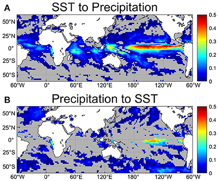
Figure 1. Normalized information flow (NIF) (A) from sea surface temperature (SST) to precipitation and (B) from precipitation to SST. Gray grid cells signify that the NIF is not significant at the 95% confidence level.

The NIF from SST to precipitation is significant in almost all tropical oceans, especially in the eastern and central Pacific. This may be due to the SST gradients' impact on the pattern of moisture convergence, which is more prominent in the tropics (Shukla and Kinter, 2006). However, there is a small region around 7◦N in the eastern Pacific that does not have significant NIFs. There are also significant SST-to-precipitation NIFs in the western tropical Pacific, which may be attributed to the high SST above the convective threshold (Graham and Barnett, 1987), but the NIFs are smaller than in the eastern Pacific, because the meridional SST gradient is relatively weak in the western Pacific (Figure 2). Some subtropical regions also show small (<0.1) but significant NIF. This is consistent with the result that SST has small but discernible effects on the atmosphere in the extratropics (Kushnir et al., 2002).

FIGURE 2

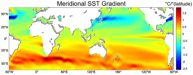
Figure 2. Global distribution of the meridional SST gradient.

In contrast, there is almost no significant NIF from precipitation to SST in tropical and subtropical regions (Figure 1). However, significant NIFs are found in a small portion of the eastern Pacific, where the shortwave radiation-SST feedback is known to serve as a negative feedback. The NIF from precipitation to SST is significant mainly in the extratropics. This result is in agreement with Frankignoul (1985), who concluded that the atmosphere drives the SST over the extratropics.

Local drivers

Since the value of NIF can represent the magnitude of the interactions between the ocean and the atmosphere, we can consider that the ocean is the primary driver in the local ocean-atmosphere coupling system if the NIF from SST to precipitation were larger than the NIF from precipitation to SST in a grid point, and vice versa. To quantify the relative importance of two-way interactions, we introduce

$\begin{array}{ll}{\text{C}}_{\text{local}}=\frac{{\text{τ}}_{\text{SST}\to \text{Pre}}-{\text{τ}}_{\text{Pre}\to \text{SST}}}{{\text{τ}}_{\text{SST}\to \text{Pre}}+{\text{τ}}_{\text{Pre}\to \text{SST}}}& (17)\end{array}$

where τ_SST→Pre is the magnitude of NIF from SST to precipitation and τ_Pre→SST is the magnitude of NIF from precipitation to SST. An area is primarily driven by the atmosphere if −1 ≤C_local <0, and by the ocean if 0 <C_local ≤ 1.

Figure 3 reveals that C_local shows considerable positive values in the tropics and negative values among the extratropics. This suggests that the ocean is the dominant driver in the tropical ocean-atmosphere system, while the atmosphere mainly drives the ocean in the extratropics. This is consistent with Bach et al. (2019), who have drawn a similar conclusion using the Granger causality.

FIGURE 3

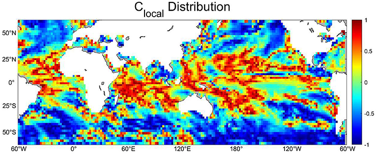
Figure 3. Magnitude of C_local. Positive values indicate that the ocean-to-atmosphere influence is more dominant, while negative values signify that the atmosphere-to-ocean influence is more dominant.

Latitudinal variation of NIFs

Since a strong latitudinal dependence for NIFs is seen in Figures 1, 3, we calculate the zonal average of NIFs at different latitudes in both directions (Figure 4). It is shown that NIFs in both directions reach their peak near the equator and rapidly decrease with increasing latitude in the tropics, but then they flatten out in the mid-latitudes. The high NIF peak in both directions indicates that the ocean and the atmosphere are strongly coupled with each other near the equator. Also, the SST-to-precipitation NIFs are higher than equatorward of about 30◦N and 30◦S, while the precipitation-to-SST NIFs are higher on the poleward side, in agreement with past literatures (Bach et al., 2019). Interestingly, there is an abnormal local minimum for the NIFs from SST to precipitation around 7◦N and a local maximum for the NIFs around 15◦N. The local minimum in precipitation-to-SST NIFs may be attributed to the Intertropical Convergence Zone (ITCZ), which is located to the north of the equator around 5◦N in its mean. We hypothesise that the ITCZ may restrain the effect from SST to precipitation, which results in a local minimum of SST-to-precipitation NIFs around 7◦N and therefore a local maximum around 15◦N. Also, there is a slight interhemispheric asymmetry; the peak of the SST-to-precipitation NIFs is located slightly to the north of the equator, while the peak of precipitation-to-SST NIFs appears south of the equator. The northward shift of the peak of SST-to-precipitation may be attributed to the higher SST north of the equator, but the reason for the southward shift of the peak in precipitation-to-SST NIFs is not clear.

FIGURE 4

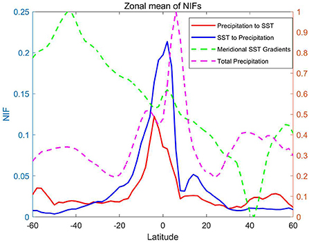
Figure 4. Zonal average of NIFs at different latitudes. The red (blue) curve shows NIFs from precipitation (SST) to SST (precipitation). The meridional SST gradient (green) and the total precipitation (magenta) data is also shown. The meridional SST gradient and total precipitation are normalized to [0, 1] by calculating ${\text{y}}_{\text{i}}=\frac{{\text{X}}_{\text{i}}-{\text{X}}_{min}}{{\text{X}}_{max}-{\text{X}}_{min}}$.

Remote analyses

Remote NIFs

Since SST in one place may be influenced by atmospheric convection in a remote area and vice versa via teleconnections, we compute the NIFs from SST in all other grid points to precipitation in one grid point and from precipitation in all other grid points to SST in one grid point. Figure 5A shows the maximum SST-to-precipitation NIFs. All regions show significant NIFs from somewhere. The NIFs in the tropical Pacific, particularly in the central and western tropical Pacific, are relatively high. Besides, the western and eastern tropical Indian Ocean also show relatively high NIFs. On the other hand, NIFs in the extra-tropics are lower than 0.2. Precipitation over regions with low maximum NIFs are not strongly influenced by SST anywhere on the globe and may be associated with atmospheric internal variability. Thus, precipitation anomalies in such regions may be less predictable. For the maximum NIFs from precipitation to SST (Figure 5B), the most prominent part is also located in the central and eastern Pacific, although relatively high NIFs of around 0.4 are found in some regions in the extra-tropics.

FIGURE 5

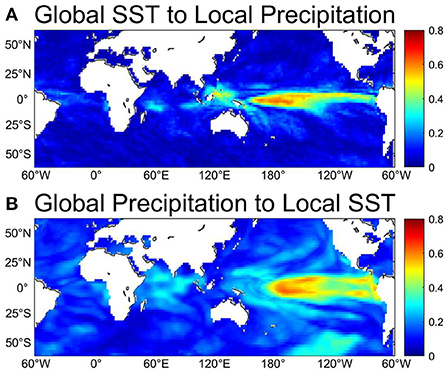
Figure 5. Maximum remote NIFs (A) from global SST to local precipitation and (B) from global precipitation to local SST.

Remote driver

To compare the magnitude of remote and local influences, the ratio of the local and maximum remote NIFs is computed (Figure 6). It is shown that the local impact from SST to precipitation is dominant in almost all tropical regions. For the precipitation-to-SST NIFs, remote impacts are much stronger except for a small area in the central-eastern equatorial Pacific and southeastern tropical Indian Ocean. Also, some regions, such as the northwestern and southeastern Indian Ocean, eastern equatorial and northwestern Atlantic, and most of the equatorial Pacific, show apparently larger remote NIFs from SST to precipitation. We will discuss where those large remote NIFs come from for these specific regions in the next subsection.

FIGURE 6

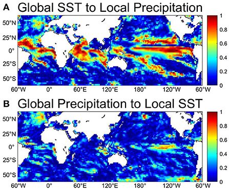
Figure 6. Ratio for the local and maximum remote NIFs (A) from global SST to local precipitation and (B) from global precipitation to local SST. The relative importance of local impact becomes increasingly large as the value approaches one.

Regional analyses

To better understand the interactions between the atmosphere and the ocean in regions with relatively large NIFs, we select six representative regions: The Niño-3 region in the eastern equatorial Pacific (150–90◦W, 5◦N−5◦S), the western equatorial Pacific (120–140◦E, 5◦N−5◦S), the southeastern tropical Indian Ocean that corresponds to the eastern pole of the Indian Ocean Dipole (IOD; 90–110◦E, 10◦S−0◦), the northwestern tropical Indian Ocean (40–60◦E, 0◦-15◦N), the Atl-3 region in the eastern equatorial Atlantic (20◦W−0◦, 3◦N−3◦S), and the northwestern Atlantic Ocean (55–30◦W, 22–7◦N).

Figure 7 shows the monthly average of NIFs. For both directions, NIFs in the Niño-3 region are generally higher than the others, and they are particularly high in October, in agreement with the development of the ENSO. This suggests that strong ocean-atmosphere coupled interactions contribute to the development of the most dominant mode of interannual climate variability (i.e., ENSO). In addition, the SST-to-precipitation NIF is more than twice as strong in April when the ENSO often start to develop, suggesting that ocean-to-atmosphere influence is more important at the initial stage of its development. Although the ENSO reaches its peak in December, the SST-to-precipitation NIF in December is smaller than that in August and October, because the growth rate of ENSO reaches its maximum in boreal autumn (Stein et al., 2010; Jin et al., 2019). However, the precipitation-to-SST NIF becomes higher than the SST-to-precipitation NIF in December and February. This may be due to the cloud-shortwave radiation feedback that operates more strongly at the peak phase of the ENSO (Waliser et al., 1994). In the western equatorial Pacific, relatively higher SST-to-precipitation NIFs are found in October, which may be likewise caused by the ENSO. The higher SST-to-precipitation is also found in February. In the southeastern and northwestern tropical Indian Ocean, NIFs may be influenced by the seasonality of the IOD, which generally develops in boreal summer and reaches its peak in autumn (Saji et al., 1999; Saji and Yamagata, 2003). In particular, NIFs in both directions over the southeastern tropical Indian Ocean are high in October. In the Atlantic, the NIFs in February are smaller for both directions. For the ATL3 region, the precipitation-to-SST NIFs are higher from April to August, while SST-to-precipitation NIFs are higher in October. The seasonality may be related to Atlantic Niño that peaks in boreal summer and the zonal mode that peaks in November and December (Okumura and Xie, 2006). On the other hand, the SST-to-precipitation NIF peaks in June and precipitation-to-SST NIF reaches its maximum in October for the northwestern Atlantic. These seasonal variations in NIFs may be linked with the seasonality of the Atlantic Meridional Mode that peaks in late boreal spring (Doi et al., 2010).

FIGURE 7

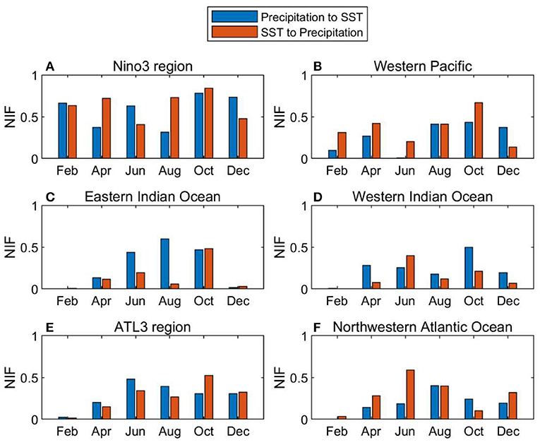
Figure 7. NIFs between regional average SST and precipitation for February, April, June, August, October, and December in (A) the Niño-3 region (150–90◦W, 5◦N−5◦S), (B) the western equatorial Pacific (120–140◦E, 5◦N−5◦S), (C) the southeastern tropical Indian Ocean (90–110◦E, 10◦S−0◦), (D) the northwestern tropical Indian Ocean (40–60◦E, 0◦-15◦N), (E) the ATL3 region(20◦W–0◦, 3◦N−3◦S), and (F) the northwestern Atlantic Ocean (55–30◦W, 22–7◦N). The blue (red) bar shows NIFs from precipitation (SST) to SST (precipitation).

We then compute NIFs from SST anomalies in every grid point to the average precipitation anomalies over the six selected regions (Figures 8–13). It can be seen that most regions present significant NIFs from the local SST. Significant local NIFs are found in February, April, and October for the eastern equatorial Pacific (Figure 8), and throughout the year except in December for the western equatorial Pacific (Figure 9). For the southeastern tropical Indian Ocean (Figure 10), significant local NIFs are found in June, August, and October, which are in agreement with the development and peak phases of the IOD, and significant local NIFs are limited to October for the northwestern tropical Indian Ocean (Figure 11). Since atmospheric circulation over the northwestern tropical Indian Ocean is strongly influenced by the Indian monsoon and/or internal atmospheric variability, local SST may not be important for most of the year (Izumo et al., 2008), but it may have some influences in the overlying atmosphere in October, possibly due to weak monsoonal wind during the monsoon break season and/or the peak phase of the IOD with anomalously warm SST enhanced precipitation during the positive IOD (Saji et al., 1999). For the ATL3 region (Figure 12), the local SST-to-precipitation NIFs are significant in April, August, October, and December, while for the northwestern Atlantic (Figure 13), the local SST shows significant impacts in April, June, and August.

FIGURE 8

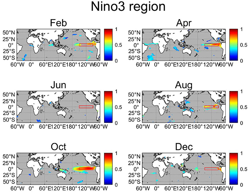
Figure 8. NIFs from remote SST to local precipitation in the Niño-3 region (red box; 150–90◦W, 5◦N−5◦S) for February, April, June, August, October, and December. Gray grid cells signify that the NIF is not significant at the 90% confidence level.

FIGURE 9

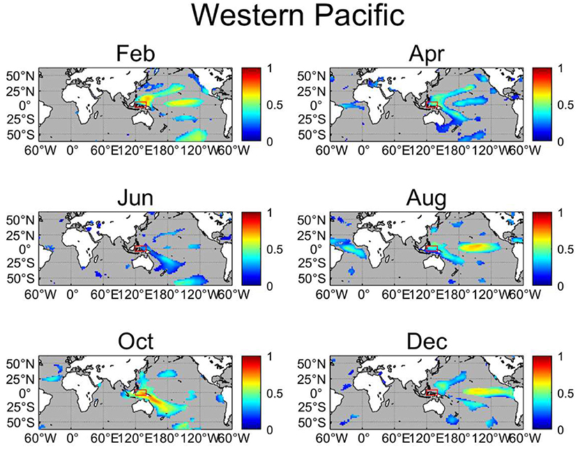
Figure 9. As in Figure 8, but for the western equatorial Pacific (120–140◦E, 5◦N−5◦S).

FIGURE 10

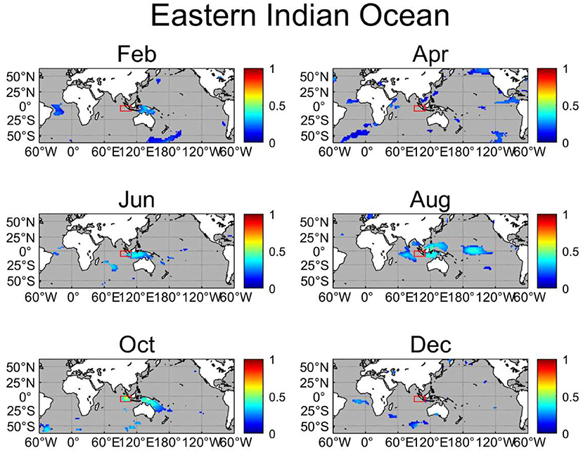
Figure 10. As in Figure 8, but for the southeastern tropical Indian Ocean (90–110◦E, 10◦S−0◦).

FIGURE 11

Figure 11. As in Figure 8, but for the northwestern tropical Indian Ocean (40–60◦E, 0◦-15◦N).

FIGURE 12

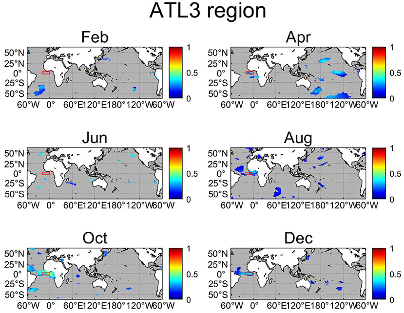
Figure 12. As in Figure 8, but for the ATL3 region (20◦W−0◦, 3◦N−3◦S).

FIGURE 13

Figure 13. As in Figure 8, but for the northwestern Atlantic Ocean (55–30◦W, 22–7◦N).

Precipitation in the above six regions is also significantly influenced by remote SST anomalies. In particular, the wide remote effects from the central Pacific may be due to the ENSO, the most dominant interannual climate mode. The Niño-3 region is affected by the Atlantic SST in April and also receives some influence from the western Pacific in August, October, and December (Figure 8). The former can be explained by the influence from the Atlantic to the ENSO events (Ham et al., 2013). As for the western equatorial Pacific, there are strong NIFs from the eastern Pacific and subtropical southwestern Pacific regions for most of the time (Figure 9), the latter of which may be related to the South Pacific Convergence Zone (SPCZ; Kiladis et al., 1989). The southeastern tropical Indian Ocean is affected by the central Pacific in August and by the Atlantic Ocean for February, April, and December as well (Figure 10). The NIFs from the Atlantic support the inference that there is some influence from the Atlantic Ocean to the Indian Ocean (Takaya et al., 2021). The northwestern tropical Indian Ocean is influenced by SST over the southeastern tropical Indian Ocean (Figure 11) due to anomalous Walker circulations associated with the IOD (Tozuka et al., 2016). The precipitation in the ATL3 region only receives remote impacts from the eastern Pacific in April (Figure 12). For the northwestern Atlantic (Figure 13), there are some significant NIFs from the Indian Ocean in June and August and from the northwestern and northeastern Pacific except for the April. Since there are no significant NIFs from the central and eastern tropical Pacific to the northwestern Atlantic, ENSO events may not have direct impacts to precipitation in this region.

Conclusions and discussions

In this study, we employ an emerging statistical method to detect the causality relations between SST and precipitation variability. We first compute NIFs between local SST and precipitation over the global oceans. It is found that the NIFs from SST to precipitation are significant in most of the tropical oceans, while the NIFs from precipitation to SST are significant mainly over the extratropics. The largest NIFs for both directions appear in the tropical Pacific (>0.5). For both directions, the magnitude of NIFs decreases with the latitude. Also, by comparing the magnitude of precipitation-to-SST and SST-to-precipitation NIFs, this study argues that the ocean drives the atmosphere more than vice versa over the tropics, while the atmosphere drives the ocean more among the extratropical oceans. This supports the earlier study by Bach et al. (2019).

Furthermore, we use NIFs to verify the teleconnections between SST and precipitation. The remote SST-to-precipitation and precipitation-to-SST NIFs are also larger in the tropical Pacific. However, precipitation seems to receive stronger local impacts from SST in the tropics, while vice versa for the extratropics. For precipitation-to-SST NIFs, the remote NIFs are much larger for most of the regions, except for a small region of the central-eastern equatorial Pacific and southeastern tropical Indian Ocean.

Also, six regions with significant NIFs are selected to calculate the NIFs from remote SST anomalies to average precipitation anomalies in those regions. The precipitation of the western Pacific is affected by not only SST of central and eastern tropical Pacific, but also the north-central and south-central Pacific, which may indicate that the western Pacific receives influences from not only the ENSO, but also from the SPCZ (Kiladis et al., 1989). However, the effect from the SPCZ region appears from April to October, but not clear in December and February, which is the peak season of the SPCZ. For the Indian Ocean, the teleconnections between the southeastern and northwestern Indian Ocean are stronger in boreal fall, and the precipitation over the southeastern Indian Ocean is also affected by the central tropical Pacific in boreal summer. For the Atlantic, the ATL3 region receives impacts from the eastern Pacific in April, while the northwestern Atlantic seems not being affected by the central and eastern Pacific.

As an extension of this study, we may compute NIFs between SST and precipitation anomalies simulated in coupled models to assess skills of these models in representing local ocean-atmosphere interactions and teleconnections. Furthermore, if such NIFs were computed and compared between historical and future scenario runs, we may study how ocean-atmosphere interactions change under global warming.

Although we have calculated NIFs between SST and precipitation, ocean-atmosphere interactions are not limited to these two variables. For example, we may compute NIFs between latent heat fluxes and SST to investigate thermodynamic air-sea coupling. If the atmosphere is driving the ocean, enhanced latent heat loss results in negative SST anomalies, but if the ocean is driving the atmosphere, positive SST anomalies generate enhanced latent heat loss. We may quantify the relative importance of ocean-to-atmosphere and atmosphere-to-ocean influences using NIFs. In addition, NIFs between wind stress curl and SST may be useful in examining the dynamical coupling (Kalnay et al., 1986). More specifically, cyclonic anomalies may induce negative SST anomalies via Ekman upwelling, whereas positive SST anomalies may be induced by anticyclonic anomalies via Ekman downwelling. On the other hand, anomalously warm SST may induce anomalous cyclone in the overlying atmosphere, while cool SST anomalies may induce anticyclonic anomalies. NIFs may be quite useful to examine their relative role.

Compared to correlation analysis or other conventional statistical methods, NIF has some advantages. Most importantly, we can easily and quantitatively estimate causality relations between different time series. In addition, the NIF has no requirement for the distribution, which means that NIF can be applied in most situations in the study of climate systems. However, we note that there are some caveats to this method. First, NIF is just a statistical method and we emphasize that results obtained by calculating NIFs should be accompanied by discussions on physical mechanisms. Also, we may only use a single lag when calculating NIFs, but some ocean-atmosphere coupled processes may not be instantaneous and have different time lags. Since we use Δt=1 month in this study, we can only catch the information flow with monthly timescales. If we want to study the causality for a longer timescale (e.g., variability associated with the Interdecadal Pacific Oscillation), we need to use larger Δt to compute NIFs.

Data availability statement

The ERA5 data and ERSST V5 data were obtained from the Asia-Pacific Data-Research Center of the International Pacific Research Center (http://apdrc.soest.hawaii.edu/data). The code of normalized information flow was uploaded by Bai in MATLAB community (https://ww2.mathworks.cn/matlabcentral/fileexchange/62471-the-normalized-information-flow?s_tid=srchtitle_information%20flow_1). The code of monthly NIF was uploaded by the first author in MATLAB community (https://ww2.mathworks.cn/matlabcentral/fileexchange/117960-the-monthly-normalized-information-flow).

Author contributions

ZY and TT contributed to the central ideas presented in the paper. ZY conducted all the analyses, prepared figures, and wrote the original draft. TT reviewed and edited the draft. All authors contributed to the article and approved the submitted version.

Funding

This study was supported by Japan Society for Promotion of Science through Grant-in-Aid for Challenging Research (Exploratory) 22K18727.

Acknowledgments

TT would like to thank Toshio Yamagata, X. San Liang, Takeshi Doi, Yushi Morioka, and Pascal Oettli for fruitful discussions on information flow. ZY would like to thank Chengzu Bai for the code of Normalized Information Flow calculations and Zoubir and Iskander for the code of bootstrap test.

Conflict of interest

The authors declare that the research was conducted in the absence of any commercial or financial relationships that could be construed as a potential conflict of interest.

Publisher's note

All claims expressed in this article are solely those of the authors and do not necessarily represent those of their affiliated organizations, or those of the publisher, the editors and the reviewers. Any product that may be evaluated in this article, or claim that may be made by its manufacturer, is not guaranteed or endorsed by the publisher.

References

Alexander, M. A., Blad,é, I., Newman, M., Lanzante, J. R., Lau, N.-C., and Scott, J. D. (2002). The atmospheric bridge: the influence of ENSO teleconnections on air–sea interaction over the global oceans. J. Clim. 15, 2205–2231. doi: 10.1175/1520-0442(2002)015<2205:TABTIO>2.0.CO;2

CrossRef Full Text | Google Scholar

Arakawa, O., and Kitoh, A. (2004). Comparison of local precipitation-SST relationship between the observation and a reanalysis dataset. Geophys. Res. Lett. 31, L12206. doi: 10.1029/2004GL020283

CrossRef Full Text | Google Scholar

Bach, E., Motesharrei, S., Kalnay, E., and Ruiz-Barradas, A. (2019). Local atmosphere–ocean predictability: dynamical origins, lead times, and seasonality. J. Clim. 32, 7507–7519. doi: 10.1175/JCLI-D-18-0817.1

CrossRef Full Text | Google Scholar

Back, L. E., and Bretherton, C. S. (2009). On the relationship between SST gradients, boundary layer winds, and convergence over the tropical oceans. J. Clim. 22, 4182–4196. doi: 10.1175/2009JCLI2392.1

CrossRef Full Text | Google Scholar

Bai, C., Zhang, R., Bao, S., San Liang, X., and Guo, W. (2018). Forecasting the tropical cyclone genesis over the Northwest Pacific through identifying the causal factors in cyclone–climate interactions. J. Atmos. Ocean. Tech. 35, 247–259. doi: 10.1175/JTECH-D-17-0109.1

CrossRef Full Text | Google Scholar

Bjerknes, J. (1969). Atmospheric teleconnections from the equatorial Pacific. Mon. Wea. Rev. 97, 163–172. doi: 10.1175/1520-0493(1969)097<0163:ATFTEP>2.3.CO;2

CrossRef Full Text | Google Scholar

Chen, M., Wang, W., Kumar, A., Wang, H., and Jha, B. (2012). Ocean surface impacts on the seasonal-mean precipitation over the tropical Indian Ocean. J. Clim. 25, 3566–3582. doi: 10.1175/JCLI-D-11-00318.1

CrossRef Full Text | Google Scholar

Christy, F. T., and Scott, A. (2013). The Common Wealth in Ocean Fisheries: Some Problems of Growth and Economic Allocation. New York, NY: Routledge.

Google Scholar

Deser, C., Alexander, M. A., Xie, S.-P., and Phillips, A. S. (2010). Sea surface temperature variability: patterns and mechanisms. Ann. Rev. Mar. Sci. 2, 115–143. doi: 10.1146/annurev-marine-120408-151453

PubMed Abstract | CrossRef Full Text | Google Scholar

Doi, T., Tozuka, T., and Yamagata, T. (2009). Interannual variability of the Guinea Dome and its possible link with the Atlantic Meridional Mode. Clim. Dyn. 33, 985–998. doi: 10.1007/s00382-009-0574-z

CrossRef Full Text | Google Scholar

Doi, T., Tozuka, T., and Yamagata, T. (2010). The Atlantic Meridional Mode and its coupled variability with the Guinea Dome. J. Clim. 23, 455–475. doi: 10.1175/2009JCLI3198.1

CrossRef Full Text | Google Scholar

Ekman, V. W. (1905). On the influence of the Earth's rotation on ocean-currents. Ark. Mat. Astron. Fys. 2, 1–52.

Google Scholar

Frankignoul, C. (1985). Sea surface temperature anomalies, planetary waves, and air-sea feedback in the middle latitudes. Rev. Geophys. 23, 357–390. doi: 10.1029/rg023i004p00357

CrossRef Full Text | Google Scholar

Garthwaite, P. H., Jolliffe, I. T., Jolliffe, I. T., and Jones, B. (2002). Statistical Inference. Oxford: Oxford University Press on Demand.

Google Scholar

Gill, A. E. (1980). Some simple solutions for heat-induced tropical circulation. Quart. J. Roy. Meteorol. Soc. 106, 447–462. doi: 10.1002/qj.49710644905

CrossRef Full Text | Google Scholar

Graham, N. E., and Barnett, T. P. (1987). Sea surface temperature, surface wind divergence, and convection over tropical oceans. Science 238, 657–659. doi: 10.1126/science.238.4827.657

PubMed Abstract | CrossRef Full Text | Google Scholar

Ham, Y. G., Kug, J. S., Park, J. Y., and Jin, F. F. (2013). Sea surface temperature in the north tropical Atlantic as a trigger for El Niño/Southern Oscillation events. Nat. Geosci. 6, 112–116. doi: 10.1038/ngeo1686

CrossRef Full Text | Google Scholar

Hersbach, H., Bell, B., Berrisford, P., Hirahara, S., Horányi, A., Muñoz-Sabater, J., et al. (2020). The ERA5 global reanalysis. Quart. J. Roy. Meteorol. Soc. 146, 1999–2049. doi: 10.1002/qj.3803

CrossRef Full Text | Google Scholar

Horel, J. D., and Wallace, J. M. (1981). Planetary-scale atmospheric phenomena associated with the Southern Oscillation. Mon. Weather Rev. 109, 813–829. doi: 10.1175/1520-0493(1981)109<0813:PSAPAW>2.0.CO;2

CrossRef Full Text | Google Scholar

Huang, B., Thorne, P. W., Banzon, V. F., Boyer, T., Chepurin, G., Lawrimore, J. H., et al. (2017). Extended reconstructed sea surface temperature, version 5 (ERSSTv5): upgrades, validations, and intercomparisons. J. Clim. 30, 8179–8205. doi: 10.1175/JCLI-D-16-0836.1

CrossRef Full Text | Google Scholar

Izumo, T., de Boyer Montégut, C., Luo, J.-J., Behera, S. K., Masson, S., and Yamagata, T. (2008). The role of the western Arabian Sea upwelling in Indian monsoon variability. J. Clim. 21, 5603–5623, doi: 10.1175/2008JCLI2158.1

CrossRef Full Text | Google Scholar

Jin, Y., Liu, Z., Lu, Z., and He, C. (2019). Seasonal cycle of background in the tropical pacific as a cause of ENSO spring persistence barrier. Geophys. Res. Lett. 46, 13371–13378. doi: 10.1029/2019GL085205

CrossRef Full Text | Google Scholar

Kalnay, E., Mo, K. C., and Paegle, J. (1986). Large-amplitude, short-scale stationary Rossby waves in the Southern Hemisphere: observations and mechanistic experiments to determine their origin. J. Atmos. Sci. 43, 252–275. doi: 10.1175/1520-0469(1986)043<0252:LASSSR>2.0.CO;2

CrossRef Full Text | Google Scholar

Karnauskas, K. (2020). Physical Oceanography and Climate. Cambridge: Cambridge University Press.

Google Scholar

Kataoka, T., Watanabe, M.T, Kimoto, M., and Tatebe, H. (2019). Wind–mixed layer–SST feedbacks in a tropical air–sea coupled system: application to the Atlantic. J. Clim. 32, 3865–3881. doi: 10.1175/JCLI-D-18-0728.1

CrossRef Full Text | Google Scholar

Kiladis, G. N., Von Storch, H., and Van Loon, H. (1989). Origin of the South Pacific convergence zone. J. Clim. 2, 1185–1195. doi: 10.1175/1520-0442(1989)002<1185:OOTSPC>2.0.CO;2

PubMed Abstract | CrossRef Full Text | Google Scholar

Klein, S. A., Soden, B. J., and Lau, N.-C. (1999). Remote sea surface temperature variations during ENSO: evidence for a tropical atmospheric bridge. J. Clim. 12, 917–932. doi: 10.1175/1520-0442(1999)012<0917:RSSTVD>2.0.CO;2

CrossRef Full Text | Google Scholar

Kohyama, T., and Tozuka, T. (2016). Seasonal variability of the relationship between SST and OLR in the Indian Ocean and its implications for initialization in a CGCM with SST nudging. Clim. Dyn. 72, 327–337. doi: 10.1007/s10872-015-0329-x

CrossRef Full Text | Google Scholar

Kosaka, Y., and Nakamura, H. (2010). Mechanisms of meridional teleconnection observed between a summer monsoon system and a subtropical anticyclone. Part II: A global survey. J. Clim. 23, 5109–5125. doi: 10.1175/2010JCLI3414.1

CrossRef Full Text | Google Scholar

Kumar, A., Chen, M., and Wang, W. (2013). Understanding prediction skill of seasonal mean precipitation over the tropics. J. Clim. 26, 5674–5681. doi: 10.1175/JCLI-D-12-00731.1

CrossRef Full Text | Google Scholar

Kushnir, Y., Robinson, W. A., Blad,é, I., Hall, N. M. J., Peng, S., and Sutton, R. (2002). Atmospheric GCM response to extratropical SST anomalies: synthesis and evaluation. J. Clim. 15, 2233–2256. doi: 10.1175/1520-0442(2002)015<2233:AGRTES>2.0.CO;2

CrossRef Full Text | Google Scholar

Li, T., and Philander, S. G. H. (1996). On the annual cycle of the eastern equatorial Pacific. J. Clim. 9, 2986–2998. doi: 10.1175/1520-0442(1996)009<2986:OTACOT>2.0.CO;2

CrossRef Full Text | Google Scholar

Li, T., Wang, B., Wu, B., Zhou, T., Chang, C.-P., and Zhang, R. (2017). Theories on formation of an anomalous anticyclone in western North Pacific during El Niño: a review. J. Meteorol. Res. 31, 987–1006. doi: 10.1007/s13351-017-7147-6

CrossRef Full Text | Google Scholar

Liang, X. S. (2008). Information flow within stochastic dynamical systems. Phys. Rev. E78, 031113. doi: 10.1103/physreve.78.031113

PubMed Abstract | CrossRef Full Text | Google Scholar

Liang, X. S. (2014). Unraveling the cause-effect relation between time series. Phys. Rev. E 90, 052150. doi: 10.1103/PhysRevE.90.052150

PubMed Abstract | CrossRef Full Text | Google Scholar

Liang, X. S. (2015). Normalizing the causality between time series. Phys. Rev. E 92, 022126. doi: 10.1103/PhysRevE.92.022126

PubMed Abstract | CrossRef Full Text | Google Scholar

Lindzen, R. S., and Nigam, S. (1987). On the role of sea surface temperature gradients in forcing low-level winds and convergence in the tropics. J. Atmos. Sci. 44, 2418–2436. doi: 10.1175/1520-0469(1987)044<2418:OTROSS>2.0.CO;2

CrossRef Full Text | Google Scholar

Matsuno, T. (1966). Quasi-geostrophic motions in the equatorial area. J. Meteorol. Soc. Japan 44, 25–43. doi: 10.2151/jmsj1965.44.1_25

CrossRef Full Text | Google Scholar

Minobe, S., Kuwano-Yoshida, A., Komori, N., Xie, S.-P., and Small, R. J. (2008). Influence of the Gulf Stream on the troposphere. Nature 452, 206–209. doi: 10.1038/nature06690

PubMed Abstract | CrossRef Full Text | Google Scholar

Mo, K. C., and Paegle, J. N. (2001). The Pacific-South American modes and their downstream effects. Int. J. Climatol. 21, 1211–1229. doi: 10.1002/joc.685

CrossRef Full Text | Google Scholar

Nakamura, H., Sampe, T., Goto, A., Ohfuchi, W., and Xie, S.-P. (2008). On the importance of midlatitude oceanic frontal zones for the mean state and dominant variability in the tropospheric circulation. Geophys. Res. Lett. 35, L15709. doi: 10.1029/2008GL034010

CrossRef Full Text | Google Scholar

Nitta, T. (1986). Long-term variations of cloud amount in the western Pacific region. J. Meteorol. Soc. Japan. 64, 373–390. doi: 10.2151/jmsj1965.64.3_373

CrossRef Full Text | Google Scholar

Nitta, T. (1987). Convective activities in the tropical western Pacific and their impact on the Northern Hemisphere summer circulation. J. Meteorol. Soc. Japan 65, 373–390. doi: 10.2151/jmsj1965.65.3_373

CrossRef Full Text | Google Scholar

Nonaka, M., and Xie, S.-P. (2003). Covariations of sea surface temperature and wind over the Kuroshio and its extension: Evidence for ocean-to-atmosphere feedback. J. Clim. 16, 1404–1413. doi: 10.1175/1520-0442(2003)16<1404:COSSTA>2.0.CO;2

CrossRef Full Text | Google Scholar

Okumura, Y., and Xie, S.-P. (2006). Some overlooked features of tropical Atlantic climate leading to a new niño-like phenomenon. J. Clim. 19, 5859–5874. doi: 10.1175/JCLI3928.1

CrossRef Full Text | Google Scholar

Pontecorvo, G., Wilkinson, M., Anderson, R., and Holdowsky, M. (1980). Contribution of the ocean sector to the United States economy. Science 208, 1000–1006. doi: 10.1126/science.208.4447.1000

PubMed Abstract | CrossRef Full Text | Google Scholar

Saji, N., and Yamagata, T. (2003). Possible impacts of Indian Ocean Dipole mode events on global climate. Clim. Res. 25, 151–169. doi: 10.3354/cr025151

CrossRef Full Text | Google Scholar

Saji, N. H., Goswami, B. N., Vinayachandran, P. N., and Yamagata, T. (1999). A dipole mode in the tropical Indian Ocean. Nature 401, 360–363. doi: 10.1038/43854

PubMed Abstract | CrossRef Full Text | Google Scholar

Semenov, M. A., and Porter, J. R. (1995). Climatic variability and the modelling of crop yields. Agric. Forest Meteorol. 73, 265–283. doi: 10.1016/0168-1923(94)05078-K

CrossRef Full Text | Google Scholar

Shukla, J., and Kinter, J. L. (2006). “Predictability of seasonal climate variations: a pedagogical review” in Predictability of Weather and Climate, eds T, Palmer., and R. Hagedorn (Cambridge: Cambridge University Press), 306–341.

Google Scholar

Silva, F. N., Vega-Oliveros, D. A., Yan, X., Flammini, A., Menczer, F., Radicchi, F., et al. (2021). Detecting climate teleconnections with Granger causality. Geophys. Res. Lett. 48, e2021GL094707. doi: 10.1029/2021GL094707

CrossRef Full Text | Google Scholar

Stein, K., Schneider, N., Timmermann, A., and Jin, F.-F. (2010). Seasonal synchronization of ENSO events in a linear stochastic model. J. Clim. 23, 5629–5643. doi: 10.1175/2010JCLI3292.1

CrossRef Full Text | Google Scholar

Stommel, H. (1948). The westward intensification of wind?driven ocean currents. Trans. Am. Geophys. Union. 29, 202–206. doi: 10.1029/TR029i002p00202

PubMed Abstract | CrossRef Full Text | Google Scholar

Stouffer, R. J., Yin, J., Gregory, J. M., Dixon, K. W., Spelman, M. J., Hurlin, W., et al. (2006). Investigating the causes of the response of the thermohaline circulation to past and future climate changes. J. Clim. 19, 1365–1387. doi: 10.1175/JCLI3689.1

CrossRef Full Text | Google Scholar

Sverdrup, H. U. (1947). Wind-driven currents in a baroclinic ocean; with application to the equatorial currents of the eastern Pacific. Proc. Nat. Acad. Sci. U. S. A. 33, 318–326. doi: 10.1073/pnas.33.11.318

PubMed Abstract | CrossRef Full Text | Google Scholar

Takaya, Y., Saito, N., Ishikawa, I., and Maeda, S. (2021). Two tropical routes for the remote influence of the northern tropical Atlantic on the Indo–Western Pacific summer climate. J. Clim.34, 1619–1634. doi: 10.1175/JCLI-D-20-0503.1

CrossRef Full Text | Google Scholar

Tozuka, T., Endo, S., and Yamagata, T. (2016). Anomalous Walker circulations associated with two flavors of the Indian Ocean Dipole. Geophys. Res. Lett. 43, 5378–5384. doi: 10.1002/2016GL068639

CrossRef Full Text | Google Scholar

Tozuka, T., and Oettli, P. (2018). Asymmetric cloud-shortwave radiation-sea surface temperature feedback of Ningaloo Niño/Niña. Geophys. Res. Lett. 45, 9870–9879. doi: 10.1029/2018GL079869

CrossRef Full Text | Google Scholar

Waliser, D. E., Blanke, B., Neelin, J. D., and Gautier, C. (1994). Shortwave feedbacks and El Niño-Southern Oscillation: Forced ocean and coupled ocean-atmosphere experiments. J. Geophys. Res. 99, 25109–25125. doi: 10.1029/94JC02297

CrossRef Full Text | Google Scholar

Wallace, J. M., and Gutzler, D. S. (1981). Teleconnections in the geopotential height field during the Northern Hemisphere winter. Mon. Wea. Rev. 109, 784–812. doi: 10.1175/1520-0493(1981)109<0784:TITGHF>2.0.CO;2

CrossRef Full Text | Google Scholar

Wang, B., Ding, Q., Fu, X., Kang, I. S., Jin, K., Shukla, J., et al. (2005). Fundamental challenge in simulation and prediction of summer monsoon rainfall. Geophys. Res. Lett. 32, L15711. doi: 10.1029/2005GL022734

CrossRef Full Text | Google Scholar

Wang, C. (2002a). Atlantic climate variability and its associated atmospheric circulation cells. J. Clim. 15, 1516–1536. doi: 10.1175/1520-0442(2002)015<1516:ACVAIA>2.0.CO;2

CrossRef Full Text | Google Scholar

Wang, C. (2002b). Atmospheric circulation cells associated with the El Niño–Southern Oscillation. J. Clim. 15, 399–419. doi: 10.1175/1520-0442(2002)015<0399:ACCAWT>2.0.CO;2

CrossRef Full Text | Google Scholar

Wang, C. (2019). Three-ocean interactions and climate variability: a review and perspective. Clim. Dyn. 53, 5119–5136. doi: 10.1007/s00382-019-04930-x

CrossRef Full Text | Google Scholar

Watanabe, M., and Jin, F.-F. (2002). Role of Indian Ocean warming in the development of Philippine Sea anticyclone during ENSO. Geophys. Res. Lett. 29, 116-1–116–4. doi: 10.1029/2001GL014318

CrossRef Full Text | Google Scholar

Wu, B., Zhou, T., and Li, T. (2009). Contrast of rainfall–SST relationships in the western North Pacific between the ENSO-developing and ENSO-decaying summers. J. Clim. 22, 4398–4405. doi: 10.1175/2009JCLI2648.1

CrossRef Full Text | Google Scholar

Wu, R., and Kirtman, B. P. (2007). Regimes of seasonal air–sea interaction and implications for performance of forced simulations. Clim. Dyn. 29, 393–410. doi: 10.1007/s00382-007-0246-9

CrossRef Full Text | Google Scholar

Xie, S.-P., Hu, K., Hafner, J., Tokinaga, H., Du, Y., Huang, G., et al. (2009). Indian Ocean capacitor effect on Indo–Western Pacific climate during the Summer following El Niño. J. Clim. 22, 730–747. doi: 10.1175/2008JCLI2544.1

CrossRef Full Text | Google Scholar

Xie, S.-P., and Philander, S. G. H. (1994). A coupled ocean–atmosphere model of relevance to the ITCZ in the eastern Pacific. Tellus 46A, 340–350, doi: 10.1034/j.1600-0870.1994.t01-1-00001.x

CrossRef Full Text | Google Scholar

Zhang, R., and Delworth, T. L. (2007). Impact of the Atlantic multidecadal oscillation on North Pacific climate variability. Geophys. Res. Lett. 34, L23708. doi: 10.1029/2007GL031601

CrossRef Full Text | Google Scholar