Temperature forecasts for the continental United States: a deep learning approach using multidimensional features

1 Introduction

Weather forecasts play a significant role in the modern economy and society. Temperature predictions, in particular, are crucial for agriculture production, water management, power generation, and emergency preparedness (Miller et al., 2008; Pathak et al., 2018; Benmarhnia et al., 2019; Johannesen et al., 2019; Sanchez et al., 2020; Nie et al., 2021). Currently, temperature forecasts are often produced using numerical weather prediction (NWP) models. NWP models are a huge success in weather forecasting and have been widely applied for predicting hurricanes, cyclones, heatwaves, and cold spells with reasonable accuracy (Bauer et al., 2015). The enhanced performance of the NWP models over the years is partially attributed to data assimilation techniques, fine-resolution observational data from various satellite products, and increasing computational resources (Sun et al., 2014; Eyre et al., 2020). While progress has also been made in improving the efficiency of the NWP models, there are still challenges that limit their capacity (Goger et al., 2016; Dueben and Bauer, 2018). Briefly, the NWP models are built based on physical mechanisms of terrestrial, oceanic, and atmospheric processes using numerical equations to predict the future state of the atmosphere (Coiffier, 2011). The spatial scale of Earth system components is large. NWP models use parametrization schemes in numerical simulations to approximate such large physical processes (Bauer et al., 2015) that uncertainties in the model outputs are unavoidable (Moosavi and Sandu, 2018). To name a few, the sources of uncertainties in NWP models include the imperfect representations of boundary conditions, cloud processes, grid resolutions, and land-ocean–atmosphere interactions (Olafsson and Bao, 2020). In addition, NWP models become computationally expensive when representing the finer details of the earth system components (Zängl et al., 2015). As a result, alternative approaches have been developed to complement the weather forecasts at longer lead times (Dueben and Bauer, 2018).

NWP models are the primary tools in weather forecasting and have been widely used for operational forecasts around the world. Some of the most applied NWP models are the Global Forecast System (GFS) developed by the National Centers for Environmental Protection (NCEP) of the U.S., European Centre for Medium-Range Weather Forecasts (ECMWF) models, Global and Regional Ensemble Prediction System (MOGREPS) developed by the United Kingdom Met Office and Global Environmental Multiscale (GEM) model developed by the Canadian Meteorological Centre (CMC). In addition to the physics-based models, there are statistical approaches that are also used in weather forecasting. Statistical methods analyze historical weather data to understand patterns or relationships that can be utilized to make predictions. Some examples of statistical methods include persistence forecasting, analog methods, climatology, and machine learning. Persistence forecasting assumes that weather conditions would remain unchanged from the most recent observations. For example, if it is currently bright, the prediction calls for more of the same. This approach is effective in steady weather patterns, but it may not capture quick shifts or transitions (Mittermaier, 2008). The analog method is locating previous weather circumstances that closely reflect current weather patterns and forecasting their eventual behavior. This method is based on the identification of similar atmospheric circulation patterns, surface conditions, and other weather conditions from the past and assumes similar future forecasts (Van den Dool, 1989). The analog approach is difficult to employ since it is nearly impossible to find a perfect analog. Various meteorological features rarely align in the same positions as they did previously. Even minor changes in the current time and the analog can provide very different outcomes. Climatology is used for seasonal forecasts and is based on long-term average weather statistics for any given area to make future forecasts. The parameter estimations in statistical approaches sometimes goes to million coefficients for describing the past weather behavior (Krishnamurti et al., 2003).

Advanced statistical techniques such as machine learning offer several advantages for improving weather forecasts. Machine learning methods have proven to be successful in capturing nonlinear patterns in complex datasets from various disciplines (Chi et al., 2020; Peng and Nagata, 2020). Deep learning (DL), an advanced method of machine learning, gives unique feature extraction and data handling capabilities. DL algorithms can handle massive amounts of data while extracting meaningful representations. The pattern recognition ability of DL algorithms has driven significant contributions in the fields of computer vision, medical imaging, and natural language processing (LeCun et al., 2010, 2015; Shen et al., 2017). DL has also sparked interest in the climate science community to address challenges associated with climate models. DL models can learn intricate relationships from large amounts of meteorological data without relying on manual feature selections. Some interesting applications of machine learning in climate science include postprocessing of the outputs from the physical models for bias correction (Rasp and Lerch, 2018), downscaling coarser resolution products to finer grid resolution (Hewson and Pillosu, 2021) and improving multi-model ensemble predictions from General Circulation Models (GCMs) (Ahmed et al., 2020). More recently, deep learning architectures have shown the capability in extreme weather predictions such as heatwaves (Chattopadhyay et al., 2020; Jacques-Dumas et al., 2022), droughts (Agana and Homaifar, 2017), tropical cyclones (Wimmers et al., 2019), and hurricanes (Devaraj et al., 2021), as well as improving parameterizations to resolve small scale processes in high-resolution climate models (Brenowitz and Bretherton, 2018). They have also been used in emulating the general dynamics of atmosphere as represented by physical models, but high-quality observational data are needed to fully realize the potential of deep neural networks (Scher and Messori, 2019; Chantry et al., 2021).

Deep learning techniques have continued to expand in climate research, and a consensus is emerging that deep learning can provide promising directions to representing unresolved physical processes in climate systems (Brenowitz and Bretherton, 2018; Kurth et al., 2018; Rasp and Lerch, 2018; Bolton and Zanna, 2019; Lagerquist et al., 2019; Reichstein et al., 2019). The growing volume of climate data is ideally suited for deep neural networks to learn complex non-linear interactions among atmospheric variables (Iglesias et al., 2015). Earlier research in data-driven weather prediction includes (Dueben and Bauer, 2018) in which a convolutional neural network (CNN) was used for predicting 500 hPa geopotential height with a lead time of 120 h. They extracted the 500 hPa data from the European Centre for Medium-Range Weather Forecasts Reanalysis (ERA5) as input to the model, and the neural network was trained from 2010 to 2017 with a validation period of 10 months. Their results showed that CNN performed well in predicting geopotential height patterns. In two other studies outputs from GCM were used for training CNN to produce the next state of GCM (Scher, 2018; Scher and Messori, 2019). The inputs to the neural network were the 3-D fields from different GCMs. In Scher (2018), a simplified GCM was used whereas complex GCMs were used in Scher and Messori (2019). In both studies, the results showed that it is possible to produce long stable climate runs from deep neural networks comparable to GCMs. In another study, (Weyn et al., 2019) predicted 300, 500 and 700 hPa geopotential height using CNN. The reanalysis data from Climate Forecast System (CFS) were used as inputs to the CNN. Their forecasts performed well up to lead time of 120 h. A benchmark dataset has been created by Rasp et al. (2020) to test the performance of different machine-learning techniques for data-driven forecasting. The dataset details are discussed in Section 2. Using the benchmark dataset (Rasp et al., 2020) analyzed direct and iterative forecasts for up to 5 days with linear regression and CNN. Four variables, that is 500 hPa, temperature t850, t2m and precipitation were used in the linear regression model whereas t850 and 500 hPa were used in CNN-based forecasts. They found that CNN direct forecasts performed better and were comparable to the operational forecasts.

CNNs have been widely used with good performance in weather and climate related studies as discussed earlier, therefore in this study we used CNN to make temperature forecasts for the continental United States based on multidimensional features. The earlier data-driven approaches were mostly limited to single climate variables or single level of geopotential heights as inputs to the neural networks (Scher and Messori, 2019; Weyn et al., 2019; Rasp et al., 2020). Since meteorological variables are correlated in space and time (Grover et al., 2015), it has been suggested to use varying levels of geopotential height in combination with other atmospheric variables for improved weather forecasts (Chattopadhyay et al., 2020; Rasp et al., 2020; Jacques-Dumas et al., 2022). In this paper, we used the CNN to predict extreme surface temperatures (t2m) and geopotential height patterns with multiple atmospheric variables as inputs to our model.

Climate models integrate many atmospheric processes such as convection, advection, turbulence, cloud formation, aerosols, and chemical reactions. The prediction ability of climate models depends on millions of parameters and it’s impossible to include them all in climate models. Furthermore, as the full representation of atmosphere, land and oceanic processes in any state-of-the-art climate model is not possible due to limitations of the computing power time and resources, leveraging the power of deep learning could be beneficial for an improved weather forecasting. These deep neural networks have the potential to achieve the goal of climate models while facilitating an examination of spatial–temporal interactions among atmospheric variables with higher efficiency. In this study, we assessed how geopotential height may affect the predictability of extreme surface temperature by incorporating different levels of geopotential heights as inputs to the CNN. Geopotential heights describe the vertical distance in the atmosphere above a reference surface. It denotes the height at which a certain atmospheric pressure level exists, considering gravity, fluctuations, and mass distribution in the Earth’s atmosphere. Fluctuations in geopotential heights are associated with the development, intensification, and movement of weather systems. The vertical temperature distribution in the atmosphere is closely related to changes in geopotential height. Meteorologists use variations in geopotential heights to identify places with stable or unstable air masses. Higher geopotential heights suggest warmer, more stable weather, whereas lower geopotential heights indicate colder, perhaps more turbulent conditions (Marshall and Plumb, 2008). The dynamics of jet stream and upper-level atmospheric flow are closely linked with geopotential heights (Hall et al., 2015). The jet stream is a narrow band of high-speed meandering air current in the upper troposphere and lower stratosphere and is caused by pressure and temperature gradients in high-latitude polar regions and warmer lower latitudes (Bluestein, 1993). The shifts in jet stream influence weather patterns causing extreme temperatures such as cold waves and heat waves (Waugh et al., 2017; Manney et al., 2022; Rousi et al., 2022).

We used geopotential heights in the upper bounds of the troposphere from 100 to 250 hPa, mid-troposphere at 500 hPa, and lower levels from 750 to 925 hPa for temperature predictions along with the CNN. Most of the earlier work in this domain focused on 500 hPa as a key predictor for weather forecasts. At 500 hPa, the geopotential height provides critical information about atmospheric circulation, synoptic-scale weather systems, and teleconnections. Its analysis aids in comprehending current weather patterns, forecasting their future evolution, and developing forecast models for accurate weather forecasting. Extreme events are also associated with blocking weather events which are stationary high-pressure systems that halt the usual west-to-east flow of the atmosphere. These atmospheric blocks depending on the location and time of the year can cause extreme weather conditions such as heatwaves during summers or cold spells in winter (Buehler et al., 2011; Chan et al., 2019). The occurrence and detection of these blocking patterns are still poorly understood with the NWP models (Woollings et al., 2018) and is an open area of research. In the deep learning framework, earlier studies have suggested to use of varying levels of geopotential heights as a potential way to improve weather prediction (Chattopadhyay et al., 2020; Rasp and Thuerey, 2021; Jacques-Dumas et al., 2022). But this point has not been examined in any prior research. Therefore, in this study, each of the geopotential height levels has been used separately and in combination with other levels to identify their role in temperature predictions. We studied two extreme temperature events from the recent past to demonstrate this framework. They are the 2012 summer heatwave and the 2014 winter cold wave. Both events resulted in extreme temperatures across the U.S. and were caused by anomalous atmospheric circulations. The goal here is to apply CNN for predicting the surface temperatures during these extreme events and the associated geopotential height patterns up to 30 days ahead. Section 2 describes the data and methodology based on CNN. In section 3, results are presented. Section 4 summarizes the findings and conclusions of this study.

2 Materials and methods

2.1 Data

This study has analyzed the Weather Bench dataset. It was developed by Rasp et al. (2020) and consists of ERA5 (Hersbach et al., 2020) hourly data from 1979 to 2018 gridded to coarser resolutions of 5.625°, 2.8125° and 1.40525°. The coarse resolution is suited for our deep learning architecture due to the GPU constraints. The dataset consists of 13 vertical levels and 14 variables. We chose a surface temperature of 2 m from the earth’s surface, and it is denoted as t2m in this study. We used geopotential heights at 100 hPa, 200 hPa,500 hPa, 700 hPa, and 925 hPa, and are denoted by z100, z200, z500, z700, and z925. Additionally, we also used temperature at 850 hPa which is denoted by t850 in this study. The study domain has a latitude range from 36°N-86°N and a longitude range from 74°W-112°W.

2.2 Methodology

The proposed framework has been applied to two extreme weather events in the U.S. from the recent past to show its performance. The two events include the 2012 summer heatwave and the 2014 winter cold wave. The 2012 summer was one of the worst heatwaves in the U.S. history (Wang et al., 2014). The heatwave began at the end of June and continued through July spreading across most of the U.S. The 2014 winter was also an extreme weather event that caused record-low temperatures in the north-central and eastern U.S. For these two extreme weather events, we predicted the temperatures and geopotential height patterns from 20th June to 15th July 2012 and 1st to 8th January 2014 using our proposed framework. We used several layers of geopotential heights to represent the full spectrum of the troposphere as inputs to our framework. Specifically, these inputs to the CNN are in the following pairs shown in Table 1. Each of these pairs is tested separately to showcase the predictability of CNN. The predictions are made for 1, 3, 5, 7, 10, 15, and 30-day lead times.

Table 1

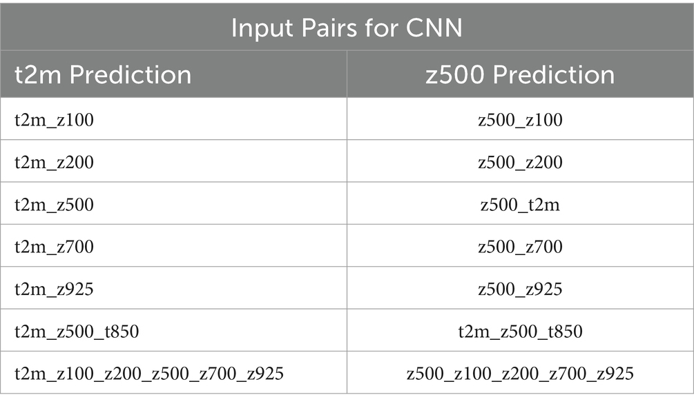
Table 1. Input Pairs for CNN.

2.3 Deep learning architecture

We used a CNN for predicting temperature and geopotential height patterns. CNN is used in many weather prediction studies (Scher and Messori, 2019; Weyn et al., 2019; Chattopadhyay et al., 2020; Rasp et al., 2020) since it is a powerful deep learning method particularly for pattern recognition tasks (LeCun et al., 2015). The CNN used in this study is based on five layers, each with 64 channels and a kernel size of 5. ReLU activation function is applied after every convolution and optimization is realized with Adams optimizer. The architecture is implemented in Python with Keras API. Each simulation is run for 25 epochs. The framework is shown in Figure 1.

Figure 1

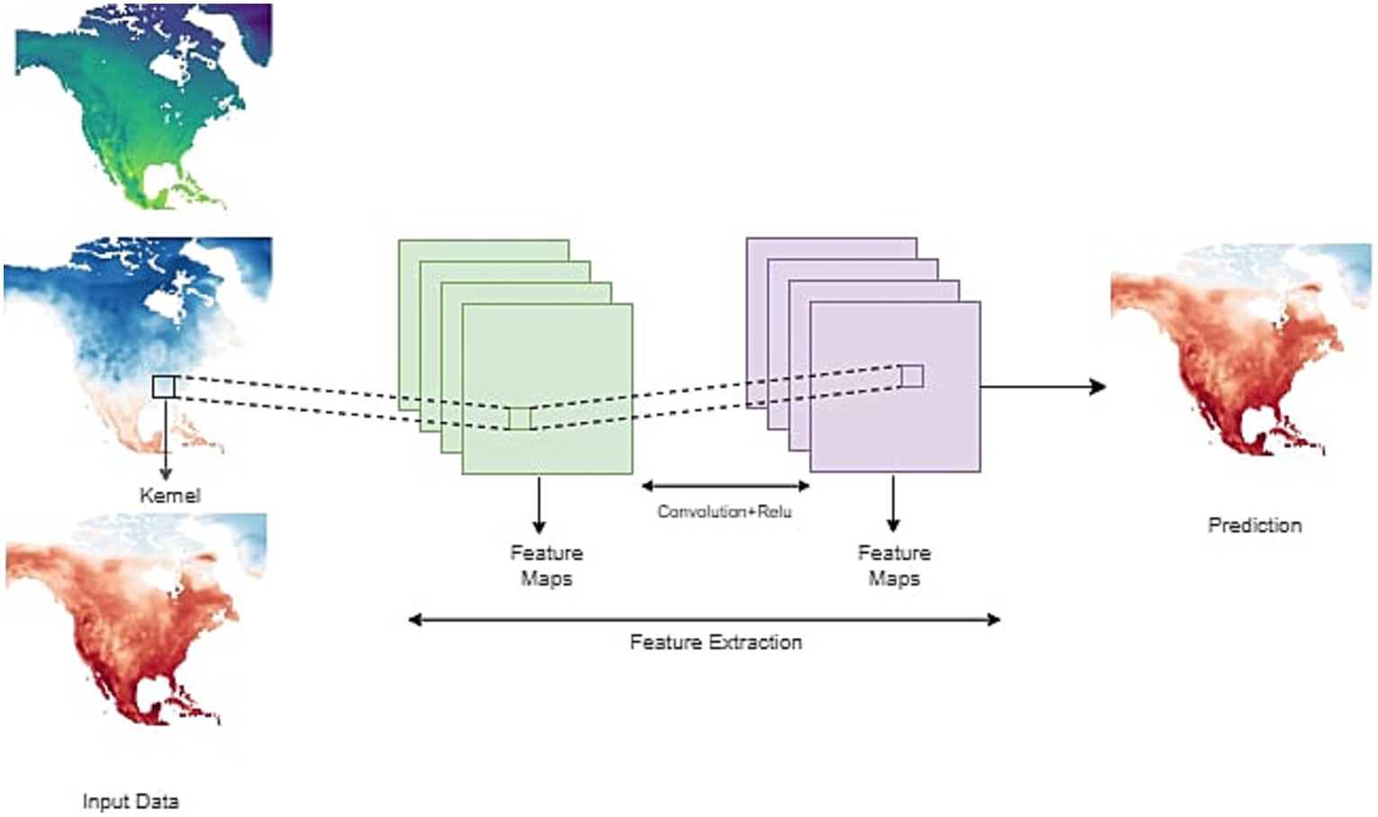
Figure 1. General schematic of CNN showing different layers of inputs, which are connected to hidden layers and output layers.

In this proposed framework, the number of layers is the input to the CNN network. The inputs can be any combination of temperature and geopotential heights. The number of inputs can be increased or decreased depending on the analysis. The output would be the desired number of meteorological variables. In our case, we used the varying levels of geopotential heights and temperatures as inputs and examined the performance of the network in producing the patterns of these variables with lead time of up to 30 days.

2.4 Training/testing data

In machine learning, it’s a practice to split the data into three parts: training, validation, and testing. For the 2012 summertime analysis, we used the training period from 1980 to 2010, validation from 2001 to 2011, and testing done for 2012. For 2014 wintertime predictions, we used a training period from 1980 to 2012, validation from 2002 to 2012, and testing done from 2013 to 2014. The testing is done on a dataset that has not been seen before during training and validation.

2.5 Evaluation metrics

Root Mean Square Error (RMSE) is used for the evaluation of the CNN performance. RMSE is the most widely used evaluation metric for testing model performance (Khanal et al., 2018; Sharma and Kakkar, 2018; Yang et al., 2019). It is defined as:

$\mathit{RMSE}=\frac{1}{N_{\mathit{predictions}}}{\displaystyle \sum }_i^{N_{\mathit{predictions}}}\sqrt{\frac{1}{N_{Iat}{N}_{\mathit{Ion}}}{\displaystyle \sum }_j^{N_{Iat}}{\displaystyle \sum }_k^{N_{\mathit{Ion}}}L\left(j\right){\left(f_{i,j,k}-t_{i,j,k}\right)}^2}$

where f is the model predictions and t are observed values. RMSE is based on mean latitude weight and L(j) is the latitude weighting factor at jth latitude index:

$L\left(j\right)=\frac{cos\left(lat\left(j\right)\right)}{\frac{1}{N_{lat}}\Sigma cos\left(lat\left(j\right)\right)}$

The predictions are made for the entire duration of the study period from June 20 to July 15 for 2012 and January 1st to 8th for 2014 and for each of the lead times and using the different combinations of inputs to the network.

3 Results

3.1 Predictions for the summertime temperature of 2012

The predictions are made with the lead times of 1, 3, 5, 7, 15 and 30 days. The 2012 summer heatwave in the US was formed due to a strong ridge of high pressure which entered from Mexico into the central plains and expanded into the western and eastern US. Several temperature records were broken during this heatwave event. Most of the high temperatures were recorded between 22 and 27 June 2012. Figure 2 shows the surface temperatures on June 23rd at 14:00 h from observation and predictions at lead times of 1, 7, 15, and 30 days. The results in Figure 1 are obtained by running the network with t2m and z500 as inputs to the network. The first column is the observation, the second column is the prediction at 1, 7, 15, and 30-day lead times and the third column is the difference in predictions from observations. The predictions for the 1-day lead time share a remarkable similarity with the observed patterns. The difference in observation and prediction for 1-day lead time varies from −6 to 1°F over the contagious U.S. The 7-day prediction patterns also matched the observations with the difference range from −9 to 1°F. The 15-day lead time values match the observed patterns with differences higher over the eastern U.S. The difference in prediction and observations for 15-day lead time varies from −9 to 1°F. The 30-day lead time also shows patterns matching observations with differences in the range of −12 to 1°F. The overall temperature predictions match well with the observations.

Figure 2

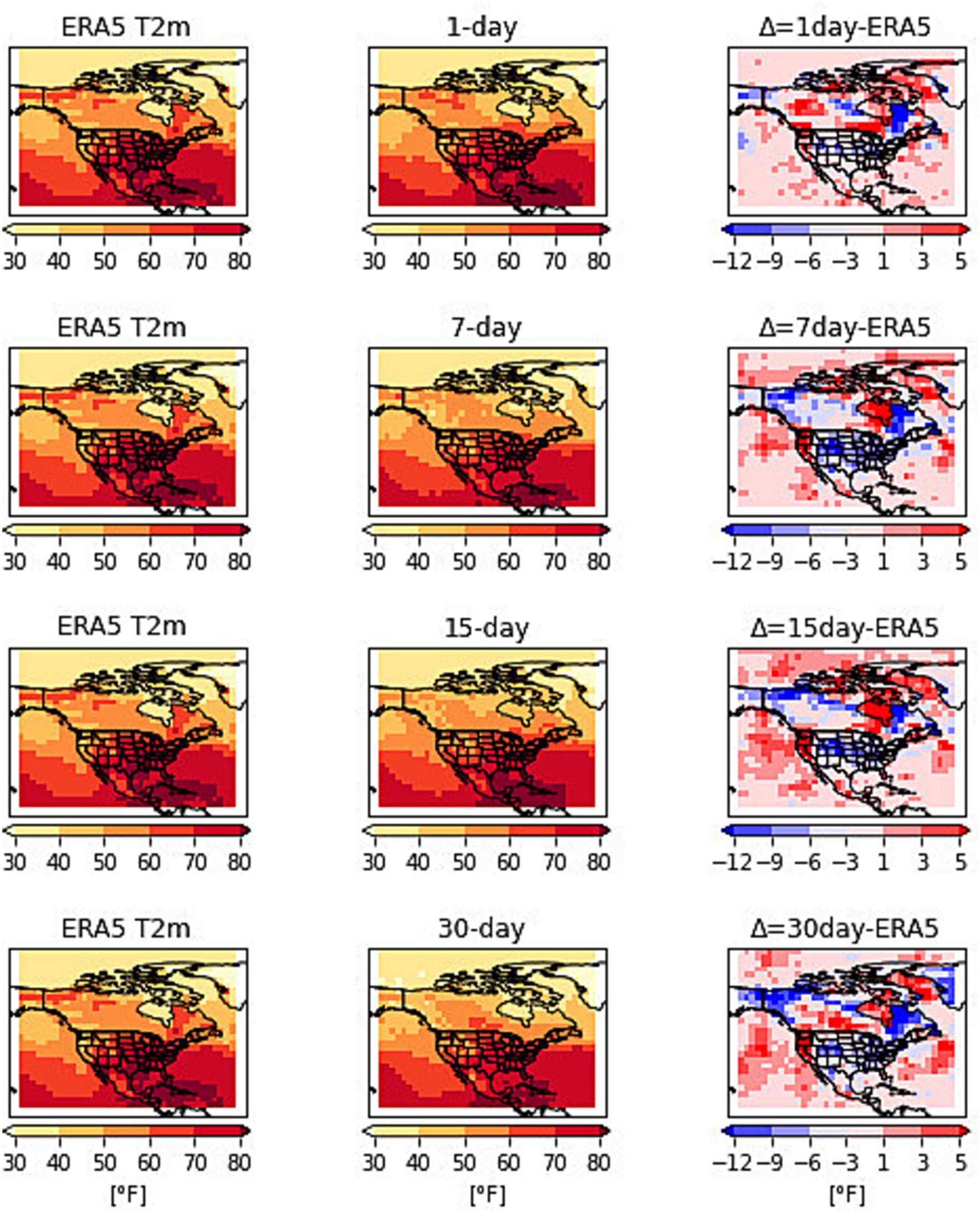
Figure 2. t2m Prediction on 23rd June 2012 with t2m and z500 as inputs to the CNN.

We tested the prediction performance of the network by increasing the number of variables as input to the network. Figure 3 shows the result of t2m prediction on the same day and time while running the network with the addition of z100, z200, z500, z700, z925, and t2m. The purpose here is to show the combined effect of upper and lower pressure levels on temperature predictions. The 1-day lead time shows temperatures matching the observations with the difference of −3 to 1°F. This difference is less than the 1-day predictions in Figure 1. The 7-day prediction shows temperature patterns match well in the eastern and western U.S. with smaller differences over the southern US. The overall difference for 7-day predictions ranges from −6 to 3°F. The 15-day predictions show lesser temperatures over the central U.S. whereas patterns match well with observations in other areas. The difference lies in the range of −6 to 3°F. The 30-day prediction also picks up spots of high temperatures and follows the overall trend of observed temperatures. The difference from observations is in the range of −9 to 3°F. Overall, the network spotted the high-temperature zones over the contiguous U.S. with high similarity to observations. The network also predicted the low temperatures over the Canadian regions during the same day and time. The network performance is greater during the first 15 days and reduces afterward.

Figure 3

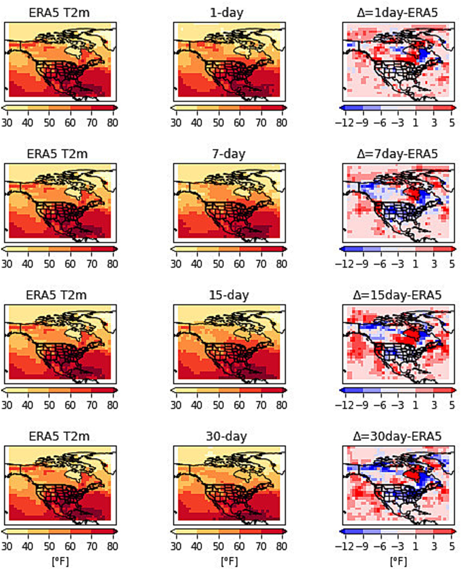
Figure 3. t2m Prediction on 23rd June 2012 with t2m and z100, z200, z500, z700 and z925 as combined input to the CNN.

Figure 4 shows the performance of each of the variables in t2m predictions using Root Mean Square Error (RMSE). The results here show the RMSE during the study period from June 20 to July 15, 2012, when the network is run for a combination of t2m and each of the pressure levels z100, z200, z500, z700, and z925 and by combing all the pressure levels for the lead time of 1, 3, 5, 7, 10, 15 and 30 days. The overall error of all the variables from 1 day to 30 days ranges from 1.4 to 2.9. The RMSE values are shown in Table 2.

Figure 4

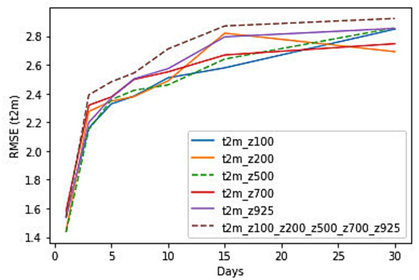
Figure 4. RMSE for t2m predictions with variable levels of geopotential heights as input to the CNN and at lead times of 1, 3, 5, 7, 10, 15 and 30 days for the time period from 20th June to 15th July 2012.

Table 2

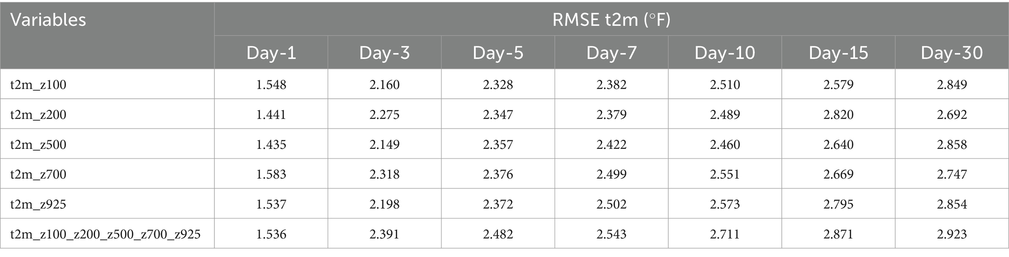
Table 2. RMSE values for t2m predictions for the time period from 20th June to 15th July 2012.

3.2 Predictions for the summertime geopotential heights of 2012

Figure 5 shows z500 patterns on June 23, 1400 h. The results in Figure 5 show the z500 predictions while running the network with z500 and t2m temperatures. The first column is the observation, the second column is the prediction at 1, 7, 15, and 30-day lead times and the third column is the difference in predictions from observations. The 1-day lead time predictions match very well with the observations. The high pressure over the central U.S. is predicted with accuracy by the network. The difference in error ranges from −300 to 300 m²s⁻². The 7-day predictions show the high-pressure patterns extending from central to all the South America. The difference in predictions ranges from −300 to 300 m²s⁻². The 15-day predictions also show most of the central and southern US under a high-pressure system. The difference in prediction range also ranges from −300 to 300 m²s⁻². The 30-day prediction also spotted high-pressure patterns over the central and southern US. The difference in predictions ranges from −100 to 300 m²s⁻². Overall, the network predicted the z500 patterns with reasonable accuracy over the central U.S. The low pressure over the Canadian region is also predicted very well.

Figure 5

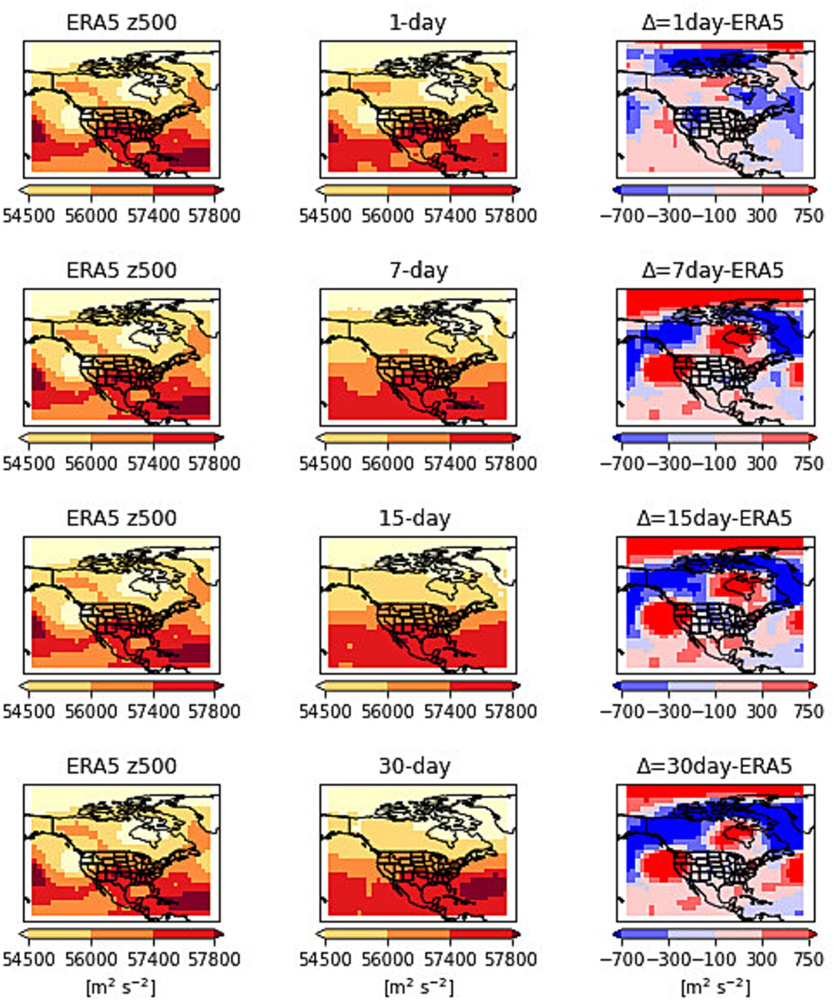
Figure 5. z500 Predictions on 23rd June 2012 with z500 and t2m as inputs to the CNN.

The combined pressure levels are also run as inputs to the network for z500 predictions shown in Figure 6. The pressure levels z100, z200, z2500, z700, and z925 are used as input to the network for prediction of z500. The 1-day prediction shows network overestimated the high pressure over the central US. The high-pressure patterns overall match well with observations. The difference in predictions varies from −300 to 100 m²s⁻². The 7-day and 15-day predictions also spotted the high-pressure areas but missed some spots of high-pressure areas. The difference in predictions ranges from −300 to 300 m²s⁻². The 30-day predictions show high pressures waning over the central US. The difference in predictions varies from most of the US -300 to 300 m²s⁻². The 30-day predictions follow the general pattern of a high-pressure system, but the network underestimates the values. The inclusion of different pressure levels changes the prediction performance of the network compared to only running the network with z500 and t2m temperatures.

Figure 6

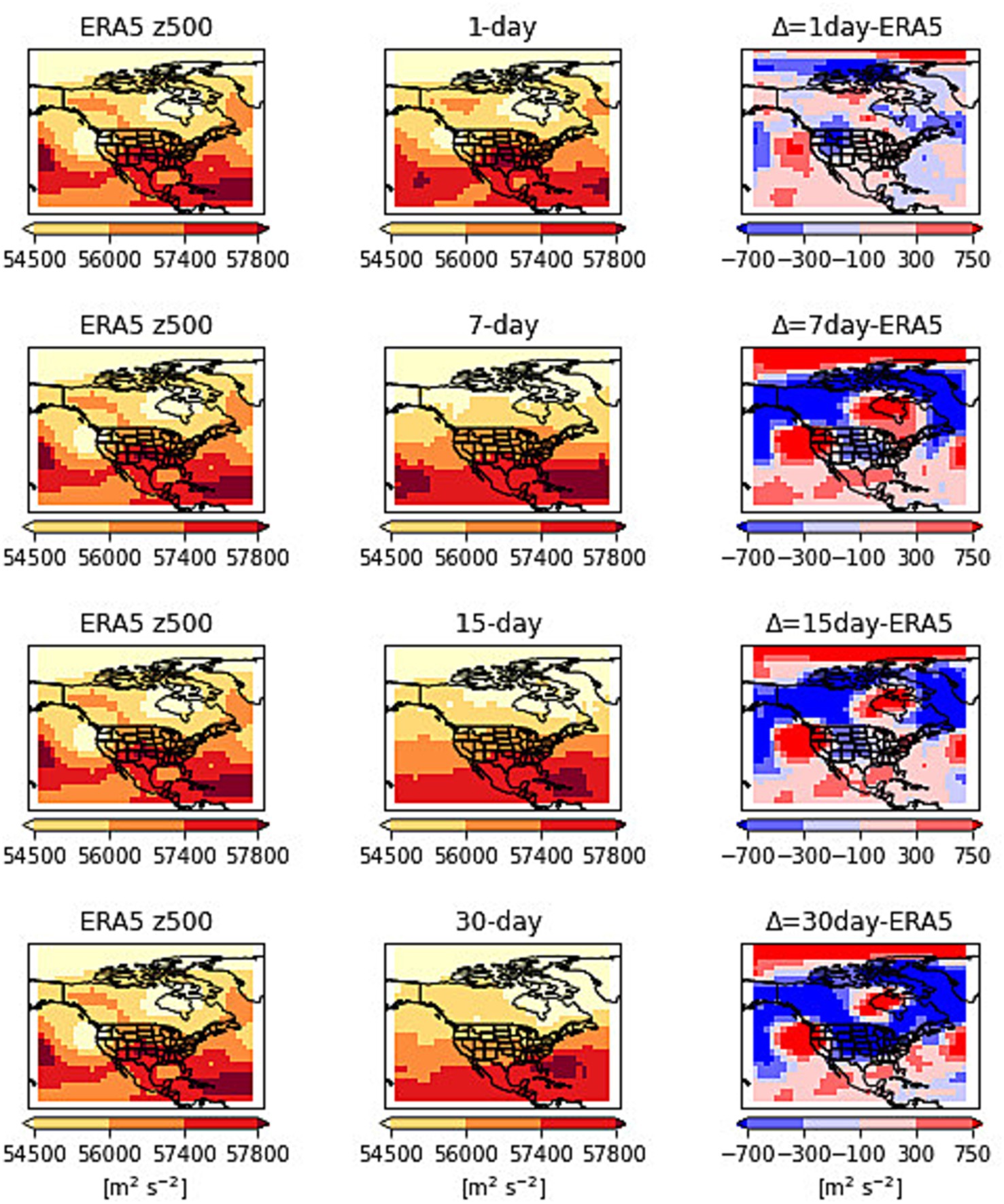
Figure 6. z500 Predictions on 23rd June 2012 with z500 and z100, z200, z500, z700 and z925 as combined input to the CNN.

The individual performance of each of the pressure levels in predicting z500 patterns is shown in Figure 7. Figure 7 shows the RMSE of z100, z200, z500, z700, z925, t2m, t850, and combined pressure levels for the study period of June 20 to July 15, 2012, and for the lead times of 1, 3, 5, 7, 10, 15 and 30 days. The results show that for 1-day to 3-day lead times the RMSE values show very slight differences. After 5-days the curves start to show different behaviors. At longer lead times the RMSE grew with all curves with larger values of z700 and z925. The lowest values are seen with t2m and t2m, t850 combinations. Table 3 shows the RMSE values for each of the combinations for z500 predictions with all lead times.

Figure 7

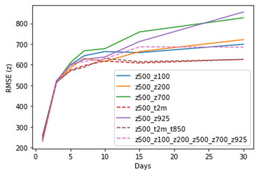
Figure 7. RMSE for z500 predictions with different variables as input to the CNN and at lead times of 1, 3, 5, 7, 10, 15, and 30 days for the time period from 20th June to 15th July 2012.

Table 3

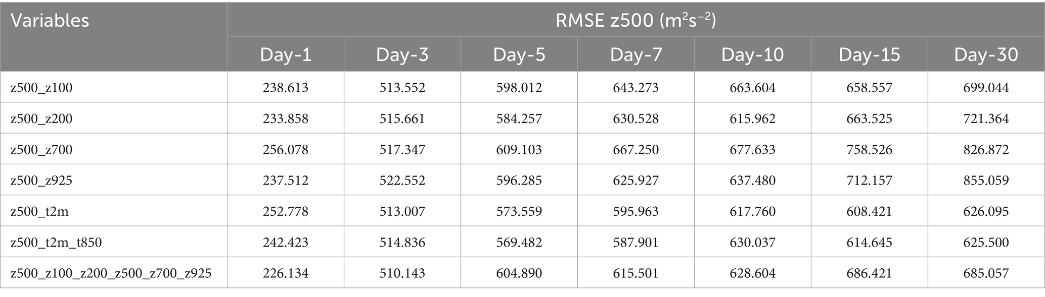
Table 3. RMSE values for z500 predictions for the time period from 20th June to 15th July 2012.

3.3 Predictions for the wintertime temperature of 2014

The performance of this framework is also tested for predicting winter temperatures. The 2014 North American cold wave was one of the most severe winters in the US marked by unusually cold temperatures, heavy snowfall, and icy conditions. The extreme cold was caused by the stretching of the polar vortex and the jet stream which brought frigid Arctic air southwards to the north, central and eastern U.S. (Cohen et al., 2022). The cold wave began in early January 2014 and lasted for several weeks. On January 6th, 2014, several cities across the Midwest and eastern US recorded their lowest temperatures. Figures 8, 9 show the t2m and z500 patterns on January 6th as observed and predicted by the network with lead times of 1, 7, 15 and 30 days. Figure 8 shows the results by running the network with t2m and z500 as inputs. The first column is the observation, the second column is the prediction at 1, 7, 15, and 30-day lead times and the third column is the difference in predictions from observations. The 1-day forecasts match well with the observations. The region from Canada to the central and eastern US could be seen covered with freezing temperatures. The 7- and 15-day forecasts show higher temperatures in central and northeastern US with increasing differences in 30-day forecasts.

Figure 8

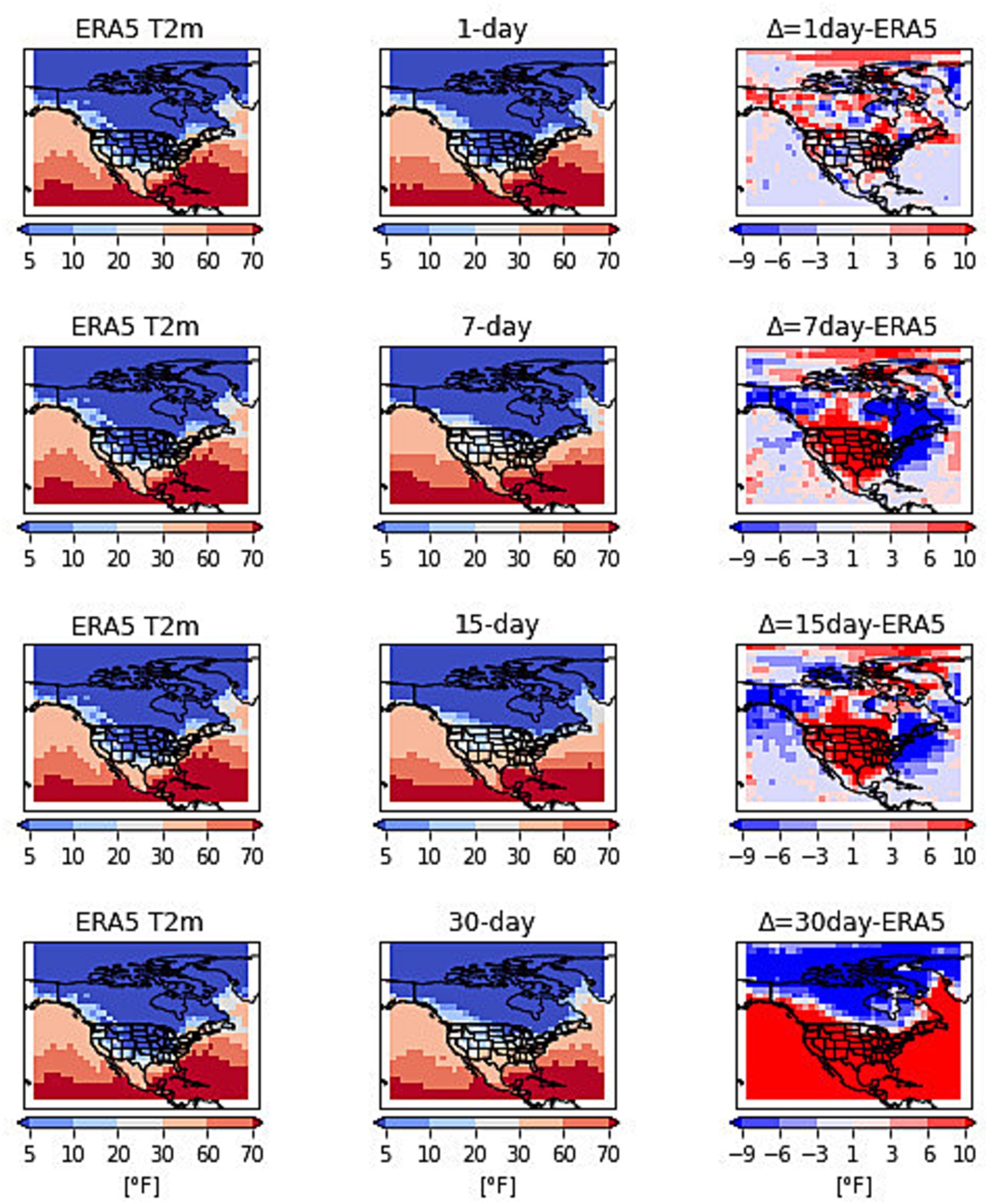
Figure 8. t2m Prediction on 6th January 2014 with t2m and z500 as inputs to the CNN.

Figure 9

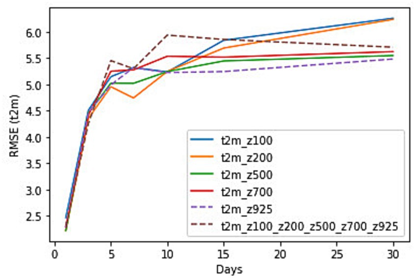
Figure 9. RMSE for t2m predictions with variable levels of geopotential heights as input to the CNN and at lead times of 1, 3, 5, 7, 10, 15 and 30 days for the time period from 1st to 8th January 2014.

The RMSE for t2m forecasts by the network as compared to the observations are shown in Figure 9 for the period from 1st to 8th January 2014. The results show the performance by running the network with t2m and vertical levels of geopotential heights as inputs. The initial performance of all input combinations shows slight variations from 1- to 3-day lead times however from 5-day onwards the error profile changes for each of the inputs. The 5 and 7-day prediction error is the least for the t2m and z200 combination which hints that z200 could be a better predictor for t2m forecasts for shorter lead times. However, at longer lead times a combination of z500, t2m, and z925, t2m shows better predictions. Supplementary Table S4 shows the RMSE values for each of the combinations for t2m predictions with all lead times.

3.4 Predictions for the wintertime geopotential heights of 2014

Figure 10 shows z500 patterns for January 6th, 2014, while running the network with z500 and z925 as inputs. Lower values of z500 are associated with cold temperatures and it could be seen that low pressure system spanned from Canada to central and eastern US bringing the cold arctic air. The 1-day lead time z500 forecasts match well with the observations. The 7-, 15- and 30-day forecasts show a high-pressure system extending upward from south America to central and eastern US. The difference in observations and forecasts varies with increasing lead times. The 1-day lead time shows very little difference in the range of −300 to 300 m²s⁻² from observations over the contagious U.S. The error grows with the increasing lead times and higher deviations over the central-eastern and western parts of the U.S. At 7- and 15-day lead times the error varies from −700 to 750 m²s⁻².

Figure 10

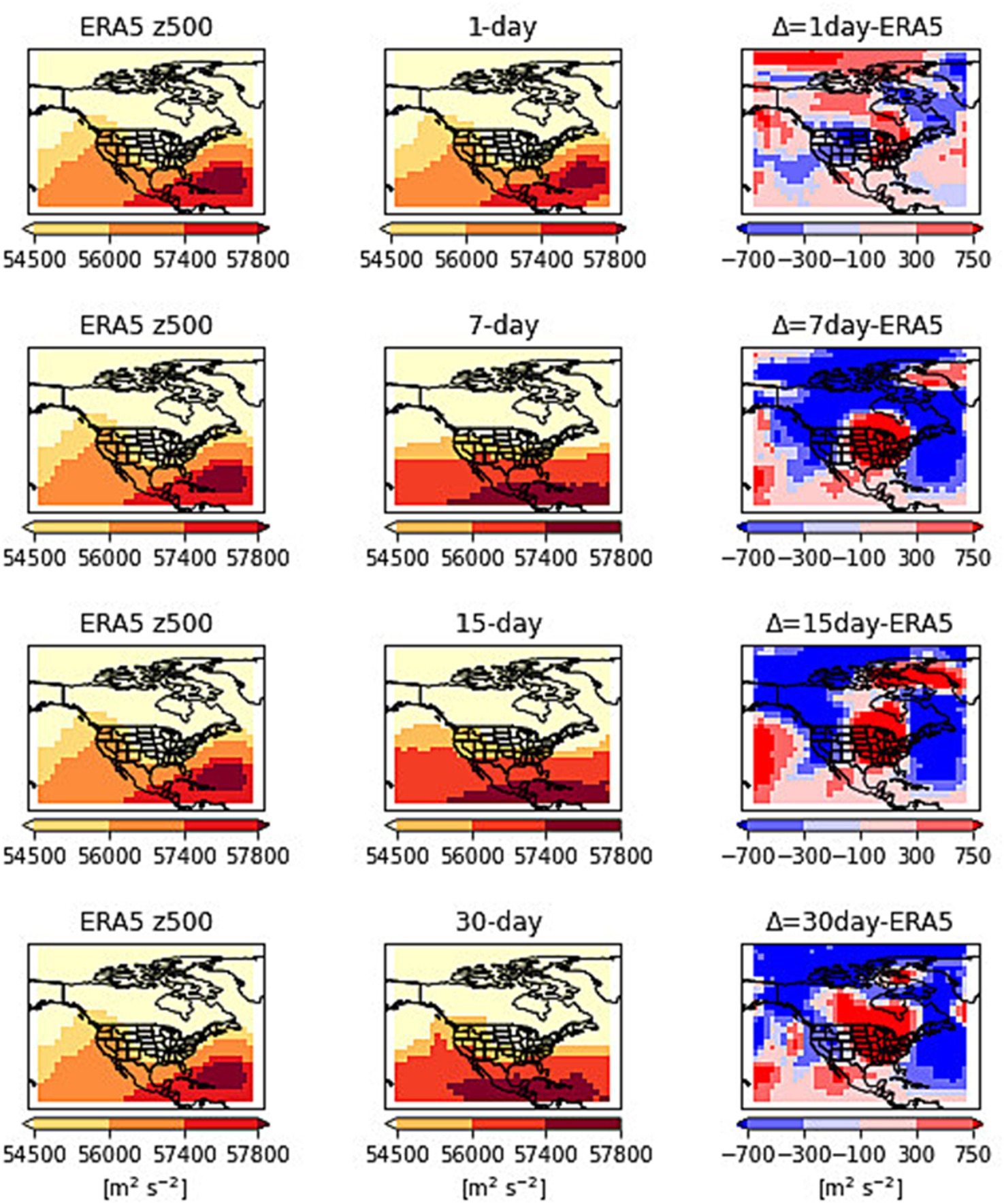
Figure 10. z500 Predictions on 6th January 2014 with z500 and z925 as inputs to the CNN.

The RMSE for each vertical level of geopotential heights for z500 predictions are shown in Figure 11 for the time period from 1st to 8th January 2014. The combination of z500 and z925 shows the least RMSE for the entire lead times. The performance of the combination of other vertical levels shows variations in RMSE for longer lead times. The combination of z500 and z100 shows the most RMSE while z200 shows less RMSE for up to 10 days lead time. The combination of t2m and z500 also shows better results for up to 15-day lead time. All vertical levels combined give slightly better results at longer lead times. Supplementary Table S5 shows the RMSE values for each of the combinations for z500 predictions with all lead times.

Figure 11

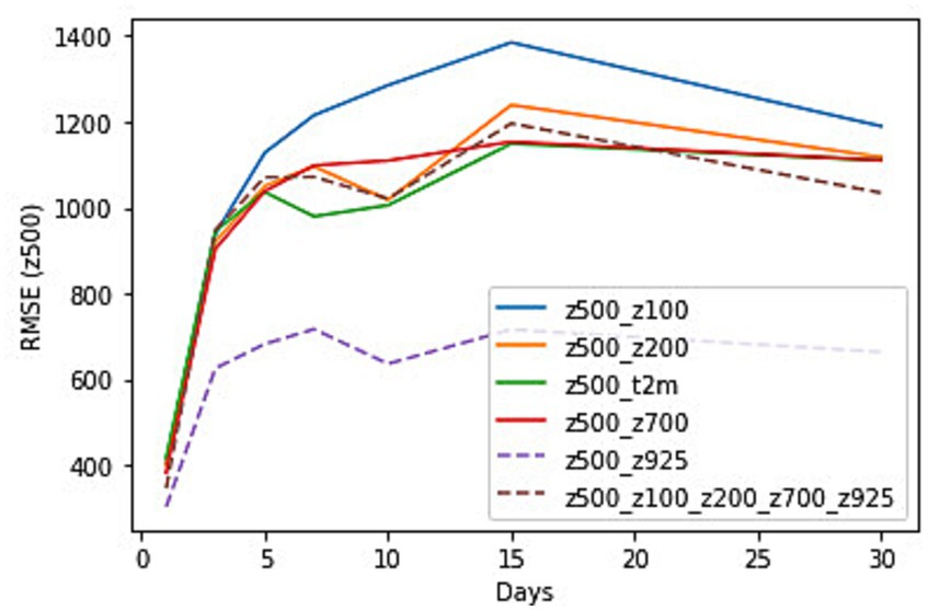
Figure 11. RMSE for z500 predictions with variable levels of geopotential heights as input to the CNN and at lead times of 1, 3, 5, 10, 15 and 30 days for the time period from 1st to 8th January 2014.

4 Discussion and conclusion

The results presented here show the performance of CNN in predicting surface temperatures (t2m) and geopotential heights during the 2012 summer heat wave and 2014 winter cold wave. The CNN with inputs from multiple layers of geopotential heights is trained with varying lead times from 1 day to 30 days. The focus of this study is to analyze the role of different levels of geopotential height in the prediction performance of CNN. Several combinations of input pairs have been used as input to CNN and RMSE is used as an evaluation metric to quantify the error in predictions.

During the summertime analysis, it was found that the combination of t2m and z500 gives better results for t2m predictions overall with less RMSE compared to other input combinations. However, at 30 days lead time, the combination of t2m and z200 shows less RMSE for t2m predictions. For the geopotential height z500 prediction, the combination of z500 and t2m and z500, t2m, and t850 give less RMSE compared to other combinations.

During the wintertime, the combination of t2m and z200 gives less RMSE for up to 7 days lead time and the combination of t2m and z925 gives better predictions for longer lead time from 10 days to 30 days. For z500 predictions during the wintertime, it has been found that the combination of z500 and z925 gives the least RMSE compared to other input pairs. The results suggest that each geopotential height contributes to t2m and z500 predictions and this study satisfies the gap in the previous studies where it has been recommended to use multiple levels of geopotential heights for improved weather predictions.

The computational costs of running deep learning models for weather forecasting can depend on the complexity of the architecture and the problem being solved. Training network on reanalysis data requires several hours of computation on high-performance graphical processing units (GPUs). Once trained the network can generate predictions in a few seconds. The performance of deep learning architectures is based on the quality of the input data. The more high-resolution long-term weather data available, the more accurate will be the prediction of the network. The new frontiers in weather forecasting are reliant on the success of resolving complexities of the atmosphere with reduced computing times and deep neural networks would make contribution to the future research.

Data availability statement

The original contributions presented in the study are included in the article/Supplementary material, further inquiries can be directed to the corresponding author.

Author contributions

JA: Investigation¸ Writing – original draft, Data curation, Formal analysis, Methodology. LC: Investigation, Writing – original draft, Conceptualization, Project administration, Supervision, Writing – review & editing.

Funding

The author(s) declare that no financial support was received for the research, authorship, and/or publication of this article.

Acknowledgments

We would like to acknowledge the University of Arkansas High-Performance Computational Center (AHPCC) for providing computational resources for this study.

Conflict of interest

The authors declare that the research was conducted in the absence of any commercial or financial relationships that could be construed as a potential conflict of interest.

Publisher’s note

All claims expressed in this article are solely those of the authors and do not necessarily represent those of their affiliated organizations, or those of the publisher, the editors and the reviewers. Any product that may be evaluated in this article, or claim that may be made by its manufacturer, is not guaranteed or endorsed by the publisher.

Supplementary material

The Supplementary material for this article can be found online at: https://www.frontiersin.org/articles/10.3389/fclim.2024.1289332/full#supplementary-material

References

Agana, N. A., and Homaifar, A. (2017). A Deep Learning Based Approach for Long-Term Drought Prediction. Conference Proceedings - IEEE SOUTHEASTCON, 1–8.

Google Scholar

Ahmed, K., Sachindra, D. A., Shahid, S., Iqbal, Z., Nawaz, N., and Khan, N. (2020). Multi-model ensemble predictions of precipitation and temperature using machine learning algorithms. Atmos. Res. 236:104806. doi: 10.1016/j.atmosres.2019.104806

PubMed Abstract | Crossref Full Text | Google Scholar

Bauer, P., Thorpe, A., and Brunet, G. (2015). The quiet revolution of numerical weather prediction. Nature 525, 47–55. doi: 10.1038/nature14956

PubMed Abstract | Crossref Full Text | Google Scholar

Benmarhnia, T., Schwarz, L., Nori-Sarma, A., and Bell, M. L. (2019). Quantifying the impact of changing the threshold of new York City heat emergency plan in reducing heat-related illnesses. Environ. Res. Lett. 14:114006. doi: 10.1088/1748-9326/ab402e

Crossref Full Text | Google Scholar

Bluestein, H. B. (1993). Observations and Theory of Weather Systems. Vol. II. Synoptic–Dynamic Meteorology in Midlatitudes. Oxford University Press Oxford, UK.

Google Scholar

Bolton, T., and Zanna, L. (2019). Applications of deep learning to ocean data inference and subgrid parameterization. J. Adv. Model. Earth Syst. 11, 376–399.

Google Scholar

Brenowitz, N. D., and Bretherton, C. S. (2018). Prognostic validation of a neural network unified physics parameterization. Geophys. Res. Lett. 45, 6289–6298. doi: 10.1029/2018GL078510

Crossref Full Text | Google Scholar

Buehler, T., Raible, C. C., and Stocker, T. F. (2011). The relationship of winter season North Atlantic blocking frequencies to extreme cold or dry spells in the ERA-40. Tellus A 63, 212–222. doi: 10.1111/j.1600-0870.2010.00492.x

Crossref Full Text | Google Scholar

Chan, P.-W., Hassanzadeh, P., and Kuang, Z. (2019). Evaluating indices of blocking anticyclones in terms of their linear relations with surface hot extremes. Geophys. Res. Lett. 46, 4904–4912. doi: 10.1029/2019GL083307

Crossref Full Text | Google Scholar

Chantry, M., Christensen, H., Dueben, P., and Palmer, T. (2021). Opportunities and challenges for machine learning in weather and climate modelling: hard, medium and soft AI. Philos. Trans. R. Soc. A Math. Phys. Eng. Sci. 379:20200083. doi: 10.1098/rsta.2020.0083

Crossref Full Text | Google Scholar

Chattopadhyay, A., Nabizadeh, E., and Hassanzadeh, P. (2020). Analog forecasting of extreme-causing weather patterns using deep learning. J. Adv. Model. Earth Syst. 12:e2019MS001958. doi: 10.1029/2019MS001958

Crossref Full Text | Google Scholar

Chi, N., Jia, J., Hu, F., Zhao, Y., and Zou, P. (2020). Challenges and prospects of machine learning in visible light communication. J. Commun. Inf. Netw. 5, 302–309. doi: 10.23919/JCIN.2020.9200893

Crossref Full Text | Google Scholar

Cohen, J., Agel, L., Barlow, M., Furtado, J. C., Kretschmer, M., and Wendt, V. (2022). The “polar vortex” winter of 2013/2014. J. Geophys. Res. Atmos. 127:e2022JD036493. doi: 10.1029/2022JD036493

Crossref Full Text | Google Scholar

Coiffier, J. (2011). Fundamentals of Numerical Weather Prediction. Cambridge: Cambridge University Press. doi: 10.1017/CBO9780511734458

Crossref Full Text | Google Scholar

Devaraj, J., Ganesan, S., Elavarasan, R. M., and Subramaniam, U. (2021). A novel deep learning based model for tropical intensity estimation and post-disaster management of hurricanes. Appl. Sci. 11:4129. doi: 10.3390/app11094129

Crossref Full Text | Google Scholar

Dueben, P., and Bauer, P. (2018). Challenges and design choices for global weather and climate models based on machine learning. Geosci. Model Dev. 11, 1–17. doi: 10.5194/gmd-2018-148

Crossref Full Text | Google Scholar

Dueben, P. D., and Bauer, P. (2018). Challenges and design choices for global weather and climate models based on machine learning. Geosci. Model Dev. 11, 3999–4009. doi: 10.5194/gmd-11-3999-2018

Crossref Full Text | Google Scholar

Eyre, J. R., English, S. J., and Forsythe, M. (2020). Assimilation of satellite data in numerical weather prediction. Part I: the early years. Q. J. R. Meteorol. Soc. 146, 49–68. doi: 10.1002/qj.3654

Crossref Full Text | Google Scholar

Goger, B., Rotach, M. W., Gohm, A., Stiperski, I., and Fuhrer, O. (2016). Current challenges for numerical weather prediction in complex terrain: topography representation and parameterizations. Int. Conf. High Perform. Comput. Simul. 2016, 890–894. doi: 10.1109/HPCSim.2016.7568428

Crossref Full Text | Google Scholar

Grover, A., Kapoor, A., and Horvitz, E. (2015). A Deep Hybrid Model for Weather Forecasting. Proceedings of the 21th ACM SIGKDD International Conference on Knowledge Discovery and Data Mining, 379–386.

Google Scholar

Hall, R., Erdélyi, R., Hanna, E., Jones, J. M., and Scaife, A. A. (2015). Drivers of North Atlantic polar front jet stream variability. Int. J. Climatol. 35, 1697–1720. doi: 10.1002/joc.4121

Crossref Full Text | Google Scholar

Hersbach, H., Bell, B., Berrisford, P., Hirahara, S., Horányi, A., Muñoz-Sabater, J., et al. (2020). The ERA5 global reanalysis. Q. J. R. Meteorol. Soc. 146, 1999–2049. doi: 10.1002/qj.3803

PubMed Abstract | Crossref Full Text | Google Scholar

Hewson, T. D., and Pillosu, F. M. (2021). A low-cost post-processing technique improves weather forecasts around the world. Commun. Earth Environ. 2, 1–10. doi: 10.1038/s43247-021-00185-9

Crossref Full Text | Google Scholar

Iglesias, G., Kale, D. C., and Liu, Y. (2015). An Examination of Deep Learning for Extreme Climate Pattern Analysis. In The 5th International Workshop on Climate Informatics (pp. 8–9).

Google Scholar

Jacques-Dumas, V., Ragone, F., Borgnat, P., Abry, P., and Bouchet, F. (2022). Deep learning-based extreme heatwave forecast. Front. Clim. 4:789641. doi: 10.3389/fclim.2022.789641

Crossref Full Text | Google Scholar

Johannesen, N. J., Kolhe, M., and Goodwin, M. (2019). Relative evaluation of regression tools for urban area electrical energy demand forecasting. J. Clean. Prod. 218, 555–564. doi: 10.1016/j.jclepro.2019.01.108

Crossref Full Text | Google Scholar

Khanal, S., Fulton, J., Klopfenstein, A., Douridas, N., and Shearer, S. (2018). Integration of high resolution remotely sensed data and machine learning techniques for spatial prediction of soil properties and corn yield. Comput. Electron. Agric. 153, 213–225. doi: 10.1016/j.compag.2018.07.016

Crossref Full Text | Google Scholar

Krishnamurti, T. N., Rajendran, K., Vijaya Kumar, T. S. V., Lord, S., Toth, Z., Zou, X., et al. (2003). Improved skill for the anomaly correlation of Geopotential Heights at 500 hPa. Mon. Weather Rev. 131, 1082–1102. doi: 10.1175/1520-0493(2003)131<1082:ISFTAC>2.0.CO;2

Crossref Full Text | Google Scholar

Kurth, T., Treichler, S., Romero, J., Mudigonda, M., Luehr, N., Phillips, E., et al. (2018). Exascale deep learning for climate analytics. In: SC18: International conference for high performance computing, networking, storage and analysis IEEE. 649–660.

Google Scholar

Lagerquist, R., McGovern, A., and Gagne II, D. J. (2019). Deep learning for spatially explicit prediction of synoptic-scale fronts. Weather and Forecasting 34, 1137–1160.

Google Scholar

LeCun, Y., Bengio, Y., and Hinton, G. (2015). Deep learning. Nature 521, 436–444. doi: 10.1038/nature14539

PubMed Abstract | Crossref Full Text | Google Scholar

LeCun, Y., Kavukcuoglu, K., and Farabet, C. (2010). Convolutional Networks and Applications in Vision. Proceedings of 2010 IEEE International Symposium on Circuits and Systems, 253–256.

Google Scholar

Manney, G. L., Butler, A. H., Lawrence, Z. D., Wargan, K., and Santee, M. L. (2022). What’s in a name? On the use and significance of the term “polar vortex”. Geophys. Res. Lett. 49:e2021GL097617. doi: 10.1029/2021GL097617

Crossref Full Text | Google Scholar

Marshall, J., and Plumb, R. A. (2008). Atmosphere, Ocean and Climate Dynamics: An Introductory Text. Vol. 93 Burlington, MA USA.

Google Scholar

Miller, N. L., Hayhoe, K., Jin, J., and Auffhammer, M. (2008). Climate, extreme heat, and electricity demand in California. J. Appl. Meteorol. Climatol. 47, 1834–1844. doi: 10.1175/2007JAMC1480.1

PubMed Abstract | Crossref Full Text | Google Scholar

Mittermaier, M. P. (2008). The potential impact of using persistence as a reference forecast on perceived forecast skill. Weather Forecast. 23, 1022–1031. doi: 10.1175/2008WAF2007037.1

Crossref Full Text | Google Scholar

Moosavi, A., and Sandu, A. (2018). A state-space approach to analyze structural uncertainty in physical models. Metrologia 55:S1. doi: 10.1088/1681-7575/aa8f53

Crossref Full Text | Google Scholar

Nie, W., Zaitchik, B. F., Rodell, M., Kumar, S. V., Arsenault, K. R., and Badr, H. S. (2021). Irrigation water demand sensitivity to climate variability across the contiguous United States. Water Resour. Res. 57:2020WR027738. doi: 10.1029/2020WR027738

Crossref Full Text | Google Scholar

Olafsson, H., and Bao, J.-W. (2020). Uncertainties in Numerical Weather Prediction. Amsterdam: Elsevier.

Google Scholar

Pathak, T. B., Maskey, M. L., Dahlberg, J. A., Kearns, F., Bali, K. M., and Zaccaria, D. (2018). “Climate change trends and impacts on California agriculture: a detailed review” in Agronomy, vol. 8 (Basel: MDPI AG). Available at: https://www.mdpi.com/journal/agronomy/editors.

Google Scholar

Peng, Y., and Nagata, M. H. (2020). An empirical overview of nonlinearity and overfitting in machine learning using COVID-19 data. Chaos, Solitons Fractals 139:110055. doi: 10.1016/j.chaos.2020.110055

PubMed Abstract | Crossref Full Text | Google Scholar

Rasp, S., Dueben, P. D., Scher, S., Weyn, J. A., Mouatadid, S., and Thuerey, N. (2020). WeatherBench: a benchmark data set for data-driven weather forecasting. J. Adv. Model. Earth Syst. 12:e2020MS002203. doi: 10.1029/2020MS002203

Crossref Full Text | Google Scholar

Rasp, S., and Lerch, S. (2018). Neural networks for postprocessing ensemble weather forecasts. Mon. Weather Rev. 146, 3885–3900. doi: 10.1175/MWR-D-18-0187.1

PubMed Abstract | Crossref Full Text | Google Scholar

Rasp, S., and Thuerey, N. (2021). Data-driven medium-range weather prediction with a Resnet Pretrained on climate simulations: a new model for WeatherBench. J. Adv. Model. Earth Syst. 13, 1–15. doi: 10.1029/2020MS002405

Crossref Full Text | Google Scholar

Reichstein, M., Camps-Valls, G., Stevens, B., Jung, M., Denzler, J., Carvalhais, N., et al. (2019). Deep learning and process understanding for data-driven Earth system science. Nature, 566, 195–204.

Google Scholar

Rousi, E., Kornhuber, K., Beobide-Arsuaga, G., Luo, F., and Coumou, D. (2022). Accelerated western European heatwave trends linked to more-persistent double jets over Eurasia. Nat. Commun. 13:3851. doi: 10.1038/s41467-022-31432-y

Crossref Full Text | Google Scholar

Sanchez, G. M., Terando, A., Smith, J. W., García, A. M., Wagner, C. R., and Meentemeyer, R. K. (2020). Forecasting water demand across a rapidly urbanizing region. Sci. Total Environ. 730:139050. doi: 10.1016/j.scitotenv.2020.139050

PubMed Abstract | Crossref Full Text | Google Scholar

Scher, S. (2018). Toward data-driven weather and climate forecasting: approximating a simple general circulation model with deep learning. Geophys. Res. Lett. 45, 12616–12622. doi: 10.1029/2018GL080704

Crossref Full Text | Google Scholar

Scher, S., and Messori, G. (2019). Weather and climate forecasting with neural networks: using general circulation models (GCMs) with different complexity as a study ground. Geosci. Model Dev. 12, 2797–2809. doi: 10.5194/gmd-12-2797-2019

Crossref Full Text | Google Scholar

Sharma, A., and Kakkar, A. (2018). Forecasting daily global solar irradiance generation using machine learning. Renew. Sust. Energ. Rev. 82, 2254–2269. doi: 10.1016/j.rser.2017.08.066

Crossref Full Text | Google Scholar

Shen, D., Wu, G., and Suk, H.-I. (2017). Deep learning in medical image analysis. Annu. Rev. Biomed. Eng. 19:221. doi: 10.1146/annurev-bioeng-071516-044442

PubMed Abstract | Crossref Full Text | Google Scholar

Sun, J., Xue, M., Wilson, J. W., Zawadzki, I., Ballard, S. P., Onvlee-Hooimeyer, J., et al. (2014). Use of NWP for Nowcasting convective precipitation: recent Progress and challenges. Bull. Am. Meteorol. Soc. 95, 409–426. doi: 10.1175/BAMS-D-11-00263.1

Crossref Full Text | Google Scholar

Van den Dool, H. M. (1989). A new look at weather forecasting through analogues. Mon. Weather Rev. 117, 2230–2247. doi: 10.1175/1520-0493(1989)117<2230:ANLAWF>2.0.CO;2

Crossref Full Text | Google Scholar

Wang, H., Schubert, S., Koster, R., Ham, Y.-G., and Suarez, M. (2014). On the role of SST forcing in the 2011 and 2012 extreme US heat and drought: a study in contrasts. J. Hydrometeorol. 15, 1255–1273. doi: 10.1175/JHM-D-13-069.1

Crossref Full Text | Google Scholar

Waugh, D. W., Sobel, A. H., and Polvani, L. M. (2017). What is the polar vortex and how does it influence weather? Bull. Am. Meteorol. Soc. 98, 37–44. doi: 10.1175/BAMS-D-15-00212.1

PubMed Abstract | Crossref Full Text | Google Scholar

Weyn, J. A., Durran, D. R., and Caruana, R. (2019). Can machines learn to predict weather? Using deep learning to predict gridded 500-hPa geopotential height from historical weather data. J. Adv. Model. Earth Syst. 11, 2680–2693. doi: 10.1029/2019MS001705

Crossref Full Text | Google Scholar

Wimmers, A., Velden, C., and Cossuth, J. H. (2019). Using deep learning to estimate tropical cyclone intensity from satellite passive microwave imagery. Mon. Weather Rev. 147, 2261–2282. doi: 10.1175/MWR-D-18-0391.1

Crossref Full Text | Google Scholar

Woollings, T., Barriopedro, D., Methven, J., Son, S. W., Martius, O., Harvey, B., et al. (2018). Blocking and its response to climate change. Curr. Clim. Chang. Rep. 4, 287–300. doi: 10.1007/s40641-018-0108-z

PubMed Abstract | Crossref Full Text | Google Scholar

Yang, M., Xu, D., Chen, S., Li, H., and Shi, Z. (2019). Evaluation of machine learning approaches to predict soil organic matter and pH using Vis-NIR spectra. Sensors 19:263. doi: 10.3390/s19020263

PubMed Abstract | Crossref Full Text | Google Scholar

Zängl, G., Reinert, D., Rípodas, P., and Baldauf, M. (2015). The ICON (ICOsahedral non-hydrostatic) modelling framework of DWD and MPI-M: description of the non-hydrostatic dynamical core. Q. J. R. Meteorol. Soc. 141, 563–579. doi: 10.1002/qj.2378

Crossref Full Text | Google Scholar