Control of Automated Guided Vehicles Without Collision by Quantum Annealer and Digital Devices

1. Introduction

Quantum annealing is a technology recently attracting attentions from both of academic and business sides. It solves the unconstrained binary quadratic programming problem (recently also termed as the quadratic unconstrained binary optimization (QUBO) problem) written as the following cost function

$\begin{array}{ll}E(\text{q})={\text{q}}^{\text{T}}Q\text{q},& (1)\end{array}$

where q is a vector of binary variables and Q is a matrix characterizing the problem to be solved. Surprisingly, QA is realized in an actual quantum device using present-day technology (Berkley et al., 2010; Harris et al., 2010; Johnson et al., 2010; Bunyk et al., 2014). We call the device performing the protocol of QA as the quantum anneler. However the optimization problem, which includes the unconstrained binary quadratic programming problem, is solved following adequate algorithm on the digital computer. In this sense, QA is not necessarily an alternative way to solve the optimization problem but it rather provides Because QA is one of the natural computing, utilizing quantum tunneling effect, which escapes from local minima into a global minimum (Kadowaki and Nishimori, 1998), compared to the conventional approach solving the optimization problem, it does without program a priori. In addition, the well-known quantum annealer, the D-Wave 2000Q, does not demand a huge amount of electric power for the computational part of the quantum devices compared to the high-performance computing. In this sense, QA is an optional way of computing, and main target of researches on QA can be searching its applicable situation in practical problems.

Unfortunately the range of applications is restricted to the case with the specific form as in Equation (1). The well-known optimization problem can be recasted by the form as in Equation (1) (Lucas, 2014), but the performance of QA is not necessarily revealed. The formulations of the specific form and QA for them have been tested such as portfolio optimization (Rosenberg et al., 2016), protein folding (Perdomo-Ortiz et al., 2012), the molecular similarity problem (Hernandez and Aramon, 2017), computational biology (Li et al., 2018), job-shop scheduling (Venturelli et al., 2015), election forecasting (Henderson et al., 2018), and machine learning (Crawford et al., 2016; Arai et al., 2018a; Khoshaman et al., 2018; Neukart et al., 2018; Ohzeki et al., 2018b; Takahashi et al., 2018). In addition, studies on implementing the quantum annealer to solve various problems have been performed (Arai et al., 2018a; Ohzeki et al., 2018a,b,b; Takahashi et al., 2018). The potential of QA might be boosted by the nontrivial quantum fluctuation, referred to as the nonstoquastic Hamiltonian, for which efficient classical simulation is intractable (Seki and Nishimori, 2012, 2015; Ohzeki, 2017; Arai et al., 2018b; Okada et al., 2019b). Most of them have not sufficed demand from practical situations as the size of the problems and time to solutions. Even one of the attractive formulations, the traffic optimization (Neukart et al., 2017), has not reached a level at the practical demand.

In a point of theoretical view, the potential performance of QA is well known. When the protocol of QA follows the quantum adiabatic condition, the ground state can be efficiently attained (Suzuki and Okada, 2005; Morita and Nishimori, 2008; Ohzeki and Nishimori, 2011b). This is not a realistic situation in performing QA in quantum devices such as D-Wave 2000Q. Thus, in the current version of quantum annealer, the attained solution is not always optimal owing to the limitations of devices and environmental effects (Amin, 2015). Although several protocols based on QA do not follow adiabatic quantum computation are proposed (Ohzeki, 2010; Ohzeki and Nishimori, 2011a; Ohzeki et al., 2011; Somma et al., 2012, the application of QA should be considered by taking account into an uncertain behavior of outputs from the quantum annealer. Recently, characteristic behavior on outputs of the quantum annealer is partially clarified. The outputs fall into a wide-flat valley of the cost function to be solved by QA rather than a sharp one (Kadowaki and Ohzeki, 2019). This fascinating property of QA is found in its application to the machine learning (Ohzeki et al., 2018a). The solutions in a wide-flat valley have robustness against the errors in the cost function. In the context of the machine learning, the errors in the cost function exist between formulations for the training and test data. However the solutions attained by QA shows good performance for the test data even although optimization is performed for the training data. In the case of formulating the optimization problem, we can not avoid the error in the cost function because we do not necessarily find the way to accomplish the desired task or we do not directly optimize the desired quantity by controlling the tunable parameters.

In the present study, we deal with the controlling problem of automated guided vehicles (AGVs), which are portable robots for moving materials in manufacturing facilities and warehouses (Ullrich, 2014; Fazlollahtabar et al., 2015; Fazlollahtabar and Saidi-Mehrabad, 2016), by use of the quantum annealer. The automated guided vehicles move along markers or wire on floors or uses vision, magnets, or lasers for navigation in a few cases. Currently, in most of factories, transportations of materials relies on AGVs and their smooth control. However, in limited-size factories, AGVs are frequently involved in traffic congestion around intersections because a large number of AGVs cross them simultaneously. Then we need a simple but smart system for controlling the AGVs without any collision. In the control of AGVs, rapid response is necessary for dealing with instantaneous changes in a system. Thus, it is expected that D-Wave 2000Q can provide a method for establishing the future infrastructure for controlling AGVs because it can output approximate solutions in a few tens of microseconds. The practical problem on facilities in actual factory has not been considered yet in the context of practical application of QA.

The remaining part of the paper is organized as follows: In the next section, we formulate the control of AGVs as the QUBO problem, which can be solved using D-Wave 2000Q. The solution does not always satisfy certain constraints for controlling AGVs, and output solutions must be postprocessed. We explain how to attain reasonable solutions via the postprocessing. In the third section, we solve the QUBO problem via D-Wave 2000Q and the corresponding integer programming via the Gurobi Optimizer (Gurobi Optimization, 2018) to check the validity of the solutions from the quantum annealer. In the following section, we report the results attained by D-Wave 2000Q and other solvers as references. In the last section, we summarize our study and discuss the direction of future work of the quantum annealer.

2. Methods

We give the Ising model or QUBO problem for controlling AGVs in this section. Below we demonstrate their movements in the Japanese actual factory following our formulation, but it is generic and not specific to individual situations. We do not formulate the entire plan as QUBO problem to control all AGVs simultaneously. This is one of the essential bottleneck of the current version of quantum annealaer. We must reduce the number of binary variables to describe the problems within the maximum number of qubits in the quantum annealer, and simplify the formulation as far as possible. We consider iterative scheme to provide an adequate route for each AGV during time period T. At time t₀, we gather information on the location, x_i, and the task, s_i, distributed to each AGV. We solve our QUBO problem and employ its solution to control the AGVs during time period T. After moving the AGVs at t₀ + T, we again gather information on the current situation and iterate the above procedure.

We focus on a controlling plan in time period T. We define the binary variable for each AGV as q_{μ, i} = 0, 1, where μ is the index for a route and i is that for an AGV. The index of the route is selected from a set of routes, M(x_i, s_i), where s_i is the given task for the i-th AGV. The index of i runs from 1 to N, which is the number of AGVs. The set of routes is constructed a priori following the tasks and the structure of the factory in which the AGVs run. One of the indicators for representing efficiency of the controlling AGVs is their waiting rate. The waiting rate is calculated by the ratio of the number of stopping AGVs and the total number of AGVs. However it is not straightforward to formulate the cost function to minimize the waiting rate. Instead we simply maximize the movements of AGVs while avoiding the collisions between them as

$\begin{array}{l}E\left(\text{q}\right)=-{\displaystyle \sum _{i=1}^N}{\displaystyle \sum _{\mu \in M\left(x_i,s_i\right)}}{d}_{\mu }{q}_{\mu ,i}\\ +{\lambda }_1{\displaystyle \sum _{i=1}^N}{\left({\displaystyle \sum _{\mu \in M\left(x_i,s_i\right)}}{q}_{\mu ,i}-1\right)}^2\\ +{\lambda }_2{\displaystyle \sum _{e\in E}}{\displaystyle \sum _{t=1}^T}{\left({\displaystyle \sum _{i=1}^N}{\displaystyle \sum _{\mu \in M\left(x_i,s_i\right)}}{F}_{\mu ,t,e}{q}_{\mu ,i}-1\right)}^2,& (2)\end{array}$

where E denotes all edges of the network along which the AGVs move in the factory, λ₁ and λ₂ are predetermined coefficients, and d_μ is the length of the route μ. The first term in Equation (2) is to achieve an efficient control of the AGVs, we define the simple cost function for increasing the total length in traveling of the AGVs. We count the total length of the routes employed by each AGV d_μq_{μ, i}. The second and third terms represent the penalties for avoiding unfeasible solutions. The second term ensures that each AGV q_{μ, i} select a single route. The third term avoids collision between different AGVs for each t, which ranges from t = 1 to t = T and each e, which denotes an edge in the routes for F_{μ, t, e} ≠ 0 in the factory. Here we define a binary quantity for characterizing the μ-th route as F_{μ, t, e} with 0 and 1. For each route, F_{μ, t, e} = 1 on the edge occupied by the selected route, μ, at time t. On the contrary, F_{μ, t, e} = 0 on the edge unoccupied by the selected route, μ, at time t.

We here add a comment on the relationship of our problem with the previous study for reducing the traffic flow of taxis in the literature (Neukart et al., 2017). The similar formulation was proposed for the traffic-flow optimization of moving taxis. However, the previous study did not consider the time dependence of F_{μ, t, e}. In the present study, we assume that the speed of the AGVs is almost constant. In addition, the AGVs can move as expected and can be predicted precisely. They did not also include the length of tours for each taxi and time dependence on movement along the tour of each taxi. In order to more clarify the connection with the previous study, let us expand the third term in Equation (2). We then obtain a quadratic term as ${\lambda }_2\sum _{e\in E}\sum _{t=1}^T{\left(\sum _{i=1}^N\sum _{\mu \in M\left(x_i,s_i\right)}{F}_{\mu ,t,e}{q}_{\mu ,i}\right)}^2$ and a linear term as $-2{\lambda }_2\sum _{i=1}^N\sum _{\mu \in M\left(x_i,s_i\right)}{d}_{\mu }{q}_{\mu ,i}$, because $\sum _{e\in E}\sum _{t=1}^T{F}_{\mu ,t,e}=d_{\mu }$. When λ₂ = 1, the first term in Equation (2) vanishes with the resultant linear term and then the cost function (2) coincides with that in the previous study. In this sense, the present study is an extension of the previous one. We apply our formulation straightforwardly to the optimization problem on the traffic flow of taxis.

Once we formulate the QUBO problem, we immediately generate the binary configurations as the outputs of the D-Wave 2000Q. We attain numerous outputs from D-Wave 2000Q for the same QUBO problem in a short time. In our case, we set the annealing time to attain a single output as 20 [μs] due to limitation of the quantum coherence time. It is thus difficult to certainly attain the ground state of the QUBO problem. In this sense, the quantum annealer does not work well for solving the optimization problem. The short annealing time is a bottleneck of the D-Wave 2000Q in a sense. However the outputs can be quickly attained. Let us here take the bottleneck as advantage of the D-Wave 2000Q. We generate many of outputs from the D-Wave 2000Q as sampling of binary configurations. The samples follow the Gibbs-Boltzmann distribution of the QUBO problem but with a finite strength of the quantum fluctuation as discussed in the literature (Amin, 2015). However, the solutions employed to control the AGVs must satisfy all constraints. We then filter out the outputs that do not satisfy the constraints from those of D-Wave 2000Q. As a result, we obtain feasible solutions without collisions and the multiple selection of routes. We check the efficiency of our postprocessed solutions in the next section to verify the capability of the D-Wave 2000Q in a limited practical application such as controlling the AGVs in factories.

We formulate the QUBO problem for the quantum annealer to contribute to the practical application appearing in various factories but we may utilize other solvers rather than the D-Wave 2000Q. In the present study, we also test the Fujitsu digital annealer (DA), which can solve the QUBO problem quickly as the D-Wave 2000Q (Tsukamoto et al., 2017; Aramon et al., 2018).

In order to check the validity of our QUBO problem, which is not a direct formulation of the efficiency controlling the AGVs, we solve it in an adequate way. Our formulation can be reformulated as the integer programming as

$\begin{array}{l}{\displaystyle \underset{\text{q}}{max}}\left\{{\displaystyle \sum _{i=1}^N}{\displaystyle \sum _{\mu \in M\left(x_i,s_i\right)}}{d}_{\mu }{q}_{\mu ,i}\right\},\\ \text{s}.\text{t}.{\displaystyle \sum _{\mu \in M\left(x_i,s_i\right)}}{q}_{\mu ,i}=1\forall i\text{ and }{\displaystyle \sum _{i=1}^N}{\displaystyle \sum _{\mu \in M\left(x_i,s_i\right)}}{F}_{\mu ,t,e}{q}_{\mu ,i}=1\forall t,\forall e.& (3)\end{array}$

We solve this integer programming by the branch and bound method via the Gurobi Optimizer (Gurobi Optimization, 2018) to confirm validity of our formulation.

We describe our whole system for controlling the AGVs in Figure 1. In order to shorten the time of the whole procedure to control the AGVs, we prepare a database that stores the set of routes when we create the QUBO during the time period T. In advance, we generate the shortest paths from an origin to a destination for each task. We divide the shortest paths into sets of several vertices at the longest vT, where v is the maximum speed of the AGVs, and store them. When we build the QUBO matrix, we only elucidate a vertex set included in a part of the shortest paths for achieving the given task beginning at x_i up to the reachable position at the end of period T. For instance, let us consider the case as in Figure 1. We take the first AGV at x₁ = 8 at t = 0, which has the shortest path of the route for achieving its task consisting of the node set {8, 9, 7, 4, 5, 6}. Then, we prepare the route set as {8}, {8, 9}, {8, 9, 7}, {8, 9, 7, 4}, {8, 9, 7, 4, 5}, and {8, 9, 7, 4, 5, 6}, which indicate “stop,” “1 step ahead,” and “2 steps ahead,” etc. The second AGV at x₂ = 1 at t = 0 has the route set at {1}, {1, 2}, {1, 2, 3}, {1, 2, 3, 4}, {1, 2, 3, 4, 5}, and {1, 2, 3, 4, 5, 6}. In order to increase the total length of the routes, two AGVs prefer to select {8, 9, 7, 4, 5, 6} and {1, 2, 3, 4, 5, 6}, respectively. However the third term in Equation (2) does not allow this solution. The overlap between two routes increases the value of f(q). The minimization of f(q) avoids collision between two AGVs and select the solution with {8, 9, 7, 4} and {1, 2, 3, 4, 5, 6}, or {8, 9, 7, 4, 5, 6} and {1, 2, 3, 4}. The solution of q comes from the D-Wave 2000Q, the digital annealer etc. in short time. As detailed below, we need to filter out the infeasible solutions satisfying the constraints for safely controlling the AGVs in practice. The whole time for the above procedure should be short for efficient control of the AGVs. We ere utilize the current version of the quantum annealer, which does not necessarily find the optimal solutions of our QUBO problem but quickly generates feasible solutions. Below we confirm availability of the D-Wave 2000Q in our proposed system by simulating the whole system utilizing the feasible solutions attained from our scheme.

FIGURE 1

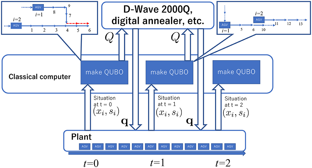
Figure 1. Our system for controlling AGVs. In the sector of classical computer, we prepare the QUBO at each time according to the current situation of the factory (x_i, s_i). For this task, we have database storing the set of routes.

3. Results

In this section, we report the results attained by iteratively solving the QUBO problem by using the D-Wave 2000Q at each time period for controlling the AGVs. For proving the efficiency of our method, we prepare a simulation environment for an actual factory as shown in Figure 2. The map is one of the actual factories in Japan. Although we below take a single map as a test of our formulation, we prepare different situations by increasing the number of AGVs and changing initial conditions. These are the essentially different situations in terms of that we attain a completely different matrix Q.

FIGURE 2

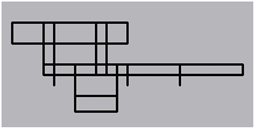
Figure 2. Factory used in the present study. In this factory, 10 AGVs move along a road and complete their tasks.

First, we test our formulation in the real setting of the actual factory. The factory usually utilizes 10 AGVs for product delivery, and the AGVs move simultaneously along four fixed routes according to predetermined tasks. We generate six candidates movement of each AGV. Thus the maximum size of the QUBO matrix is 60, which is embeddable in the D-Wave 2000Q. Notice that the QUBO matrix becomes very sparse in our formulation. Thus we further enlarge the size of the problem without an efficient embedding program (Okada et al., 2019a,c). The speed of each AGV is 0.5 m/s. The distance between nodes is 10 m.

We simulate the controlled AGV movement following the results by the following different methods. One is the conventional method, and the other is our method attained by the outputs from D-Wave 2000Q. Notice that the conventional method for controlling the AGVs is a rule-based method at every intersection in the actual factory. The rule is that when the AGVs require the same intersection route, only one AGV can move in and out at the intersection. For example, when two AGVs require the same intersection, one AGV waits until the other AGV leaves the intersection. The AGVs that move along the circumference of the factory have higher priority for entering an intersection for increasing the working rate. On the other hand, we solve the QUBO problem via D-Wave 2000Q at each time period. The time period is set to be 3 s, namely T = 3 [s]. We set the parameters as λ₁/(1 + λ₂) = 1.0 and λ₂/(1 + λ₂) = 2.0. Because D-Wave 2000Q does not deal with large elements of QUBO matrix Q_ij, the elements of the QUBO matrix is rescaled within the range of the available magnitude. D-Wave 2000Q solves the QUBO problem 1000 times for finding reasonable solutions. We filter the solutions that do not satisfy the constraints and select one of the reasonable solutions for moving the AGVs further. The AGVs move following the selected solution during the time period of 3 s. The solution indicates the movement in the next 5 s. Thus, the movement of the AGVs is updated before they reach the end of the given route.

First the results attained by the conventional method and D-Wave 2000Q are shown in Figure 3. We simulate the AGVs in the actual factory for 1,000 s and indicate the accumulated waiting time by circles. The waiting rate is calculated by the ratio of the number of stopping AGVs and the total number of AGVs. Several circles represent the locations that frequent traffic jams of the AGVs happened. The size of a circle is proportional to the accumulated waiting time of the AGVs at that point. In the case of the conventional method, the time average of the waiting rate converges to 20%. On the other hand, in the case with the D-Wave 2000Q, It can be seen from Figure 3 that the number of circles, which represent the accumulated waiting time, is considerably reduced compared to the conventional method. The time average of the waiting rate converges to 5%. The actual movement of the AGVs from an initial condition is shown in the Supplemental Video Files. Compared to the result of the conventional method, the AGVs move smoothly following the solution attained by our method with the D-Wave 2000Q. The readers can find the smooth movements of the AGVs in the Supplemental Video Files.

FIGURE 3

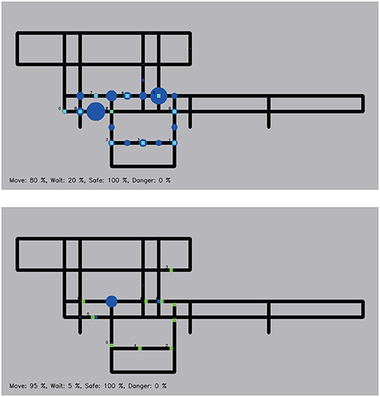
Figure 3. Comparison among the solvers: (upper) Conventional method and (bottom) D-Wave 2000Q. The green dots denote the locations of the AGVs at the end. The blue circles represent the accumulated waiting time for the AGVs.

4. Other Solvers and Validity of Formulation

It is not necessary to solve our QUBO problem using D-Wave 2000Q; one can utilize other solvers. One method is the DA, which solves the QUBO problem using an improved version of SA. Notice that the DA can solve the QUBO problem with a large number of binary variables compared to D-Wave 2000Q. The number of binary variables in our QUBO problem is 60, which is the product of the actual number of the AGVs (10) in the Japanese factory and the number of candidates of routes (6), which is set a priori so as to be embedded on the D-Wave 2000Q. Thus, the number of the binary variables is quite small. Even though the DA does not exhibit its potential efficiency in this case, we find that the time average of the waiting rate converges around 6% as shown in Figure 4. Similarly to the case with the D-Wave 2000Q, DA also leads to nice performance to control the AGVs by use of our formulation.

FIGURE 4

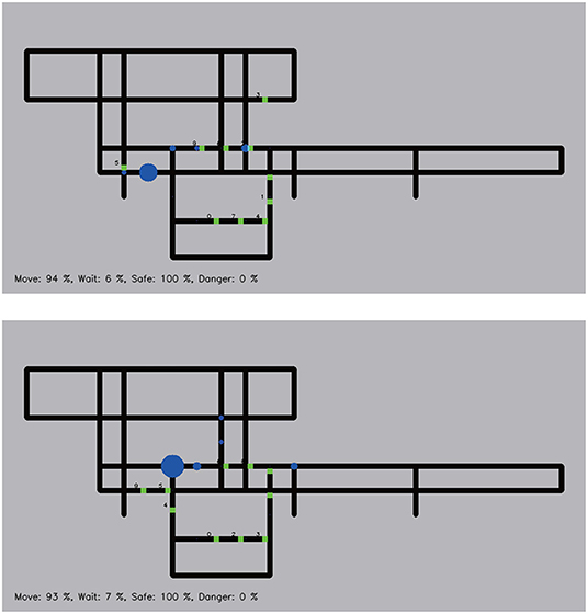
Figure 4. Comparison among the solvers: (upper) Fujitsu digital annealer and (bottom) Gurobi Optimizer as a reference. The same symbols are used in Figure 3.

In addition, in order to verify our formulation of the QUBO problem, we solve the corresponding integer programming through the relaxation of the binary variables to continuous variables by utilizing the branch and bound method via Gurobi Optimizer version 8.01 on a 4-core Intel i7 4770K processor with 32 GB RAM. In this case, we attain the optimal solution of the corresponding integer programming in a very short time and utilize the optimal solution to control the AGVs. Similarly to the previous results attained by the D-Wave 2000Q and DA, the optimal solutions controlls the AGVs without collisions. The time average of the waiting rate converges to 7%, which is slightly higher than the results of D-Wave 2000Q and DA. This is due to stochasticity of D-Wave 2000Q and the DA. The cost function itself is not necessarily a direct indicator of performance. Thus the optimal solution for the cost function is not always optimal for the actual performance in terms of the waiting rate. Similar phenomena appear in machine learning. Generalization performance, which is the measure of potential power in machine learning but not directly related to the cost function to be optimized, can be enhanced via stochastic methods to optimize cost functions. In particular, QA actually leads to better generalization performance, as shown in the literature (Ohzeki et al., 2018a). This is indirect evidence of the robustness of the solutions in the wide-flat minimum attained in the quantum annealer as reported in the literature (Kadowaki and Ohzeki, 2019).

In order to assess the typical performance of our QUBO problem, we repeat the iterative optimization for controlling the AGVs at each time period starting from the same initial condition 10 times. Because the D-Wave 2000Q and DA have stochasticity, we compute the average and maximum performance, as shown in Table 1. As shown in Table 1, the variances among the different runs are small for each solver. The Gurobi Optimizer always leads to the optimal solutions, but the waiting rates are not less than the results obtained by D-Wave 2000Q and DA. This is because the optimal solutions do not always lead to the best control of the AGVs in terms of the waiting rate. Our QUBO problem is not directly related to the waiting rate. In order to reduce the waiting rate, we add another constraint for the AGVs such that if several AGVs reach the same intersection, the AGV with more following AGVs is preferentially allowed to enter the intersection. We solve the improved integer programming with the additional constraint by employing the Gurobi Optimizer and also show its efficiency in Table 1. As shown in Table 1, the waiting rate is reduced by the improved integer programming and the result is comparable with the D-Wave 2000Q and DA with stochasticity. As well known, the integer programming can be easily improved by considering deeply the structure of the target problem. In addition, the digital computer can accept any formulation of the integer programming. This is the most advantage of the digital computer. The quantum annealer is not acceptable for an intricate QUBO problem due to the limitation of the quantum device. However our QUBO problem is simple but valuable for the quantum annealer to control the AGV in the factory, which is one of the important problems in industry. This is the first evidence showing possibility for the quantum annealer to contribute on the practical application although it has many bottlenecks to be solved.

TABLE 1

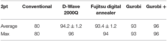
Table 1. Working rates of the AGVs obtained by the conventional method, D-Wave 2000Q, Fujitsu digital annealer, Gurobi Optimizer, and modified optimization problem for Gurobi Optimizer.

Below, we discuss the efficiency of the solvers from another point of view, the computational time. We investigate the “actual” computational time, which is obtained in a standard-user environment, and the quality of the attained solutions against the increase in the number of the AGVs and candidate routes. We prepare a hundred of different initial locations of the AGVs such as each pair of the AGVs encounter at an intersection and solve the optimization problem. We report the comparison results in average and variance below.

The D-Wave 2000Q takes 20 μs, which is predetermined by users, to once solve the optimization problem in the quantum chip with superconducting qubits. However preprocessing and postprocessing for preparation to solve the optimization problem, the latency of the network when we utilize the D-Wave 2000Q via cloud service, and the queueing time can not be avoided. Thus the actual computational time takes a little bit longer. The D-Wave 2000Q outputs many samples of the solutions once. We set the number of samples as 1,000 and measure the actual computational time. We then estimate the actual computational time per output sample as 1.39(33) ms for 9 spins, 1.33(11) ms for 21 spins, 1.51(5) ms for 30 spins, 1.45(12) ms for 39 spins, 1.90(16) ms for 51 spins, and 2.22(22) ms for 60 spins. These computational times per output sample are only to solve the QUBO problems without any assurance of precision of the attained solutions. The probability for attaining the ground state P₀ gradually decreases as the number of spins increases. In fact, P₀ = 1.00 for 9 spins, P₀ = 0.99(6) for 21 spins, P₀ = 0.97(2) for 30 spins, P₀ = 0.91(1) for 39 spins, P₀ = 0.87(2) for 51 spins and P₀ = 0.74(2) for 60 spins.

The number of binary variables consists of the multiplication of that of the AGVs and the routes. The computational time drastically increases for the case of D-Wave 2000Q beyond 60 spins. This is due to the limitation of the number of binary variables to be solved simultaneously. We solve the case with a larger number of binary variables by utilizing qbsolv, which divides the original problem into a number of small problems. To iteratively use D-Wave 2000Q, we must wait for several seconds owing to the job queue via the cloud service provided by the D-Wave systems Inc. at each iteration to solve the small problems. The actual computational time per output sample and iteration is 1.80(44) ms for 90 spins, 1.77(59) ms for 399 spins, and 1.37(53) ms for 900 spins. The iteration numbers become 2 × 10 for 90 spins, 8 × 10 for 399 spins, and 33 × 10 for 900 spins. The former number in the product is the number of division of the original large problem into small subproblems, and the latter one is that of repetition to solve the optimization problem. Thus, the actual computational time can be extremely long. In addition, the probabilities for attaining the ground state get worse as P₀ = 0.27(12) for 90 spins P₀ = 0.03(5) for 399 spins and P₀ = 0.001(9) for 900 spins. This is a weak point to employ the D-Wave 2000Q to solve the QUBO problem. Although it seems that the computational time does not depend on the number of binary variables, the probability for attaining the ground state gradually decreases as the number of binary variables increases. On the other hand, the Gurobi Optimizer leads to the optimal solutions for each case. Its computational time to attain the optimal solution depends on the number of binary variables. 2.79(6) ms for 30 spins, 3.46(5) for 60 spins 4.25(6) for 90 spins, and 8.70(6) ms for 400 spins.

On the other hand, for the DA, the machine time is set to be enough to solve the optimization problem about 8 ms. The actual computational time per output sample takes a little bit longer than the machine time as 0.216(2) s for 9 spins, 0.219(4) s for 21 spins, 0.222(6) s for 30 spins, 0.220(7) s for 39 spins, and 0.232(9) for 51 spins, 0.240(11) for 60 spins, 0.230(6) ms for 90 spins, 0.336(18) s for 399, and 0.519(32) ms for 900 spins. Up to 1,024 spins, the current version of the DA can solve once the optimization problem without dividing it into small subproblems. This is an advantage point of the DA in comparison with the D-Wave 2000Q. In addition, the probability for attaining the ground state P₀ is relatively higher compared to that of the D-Wave 2000Q as P₀ = 1.0 for 9, 21, 30, 39, and 51 spins, P₀ = 1.000(5) fpr 60 spins, P₀ = 0.97(3) for 90 spins, P₀ = 0.71(3) for 399 spins, and 0.37(12) for 900 spins. Notice that the higher value of the probability for attaining the ground state is obtained by tuning the annealing schedule. Instead, the actual computational time takes longer.

We compute the time to solutions (TTS) defined as

$\begin{array}{ll}\text{TTS}\left(p\right)=t_c\frac{log\left(1-p\right)}{log\left(1-P_0\right)},& (4)\end{array}$

where t_c is the actual computational time per output sample and p is a predetermined precision to attain the ground state. The time to solution is an indicator of the performance of the solver in the stochastic way. We show the comparison data of TTS (0.99) of the D-Wave 2000Q and the DA and the actual computational time of the Gurobi Optimizer in Figure 5. In the successful cases with P₀ = 1.0, we plot the actual computational time instead of the TTS. The actual computational time per output sample can be upper bound for the TTS.

FIGURE 5

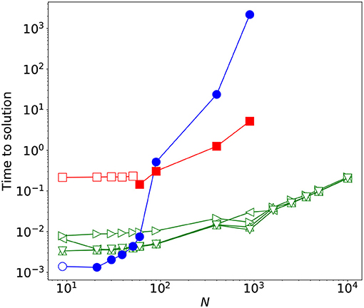
Figure 5. Comparison of the time to solution (TTS). The horizontal axis denotes the number of AGV N and the vertical one represents time to solution in seconds. The filled circles and squares denote the TTS obtained by D-Wave 2000Q and the DA, respectively. The outlined circles and squares represent the actual computational time (upper bound of the TTS) by the D-Wave 2000Q and the DA. In addition, we plot the actual computational time by the Gurobi Optimizer by the triangles. The directions of the triangles distinguish the results by different levels of the “presolve” option for the Gurobi Optimizer as “default,” “none,” “conservative,” and “aggressive”.

5. Conclusions

We formulate the QUBO problem for controlling the AGVs in the actual factory in Japan. This is the first step of the practical application of the quantum annealer to the actual situation in industry. In order to reduce the number of binary variables, which is embeddable on the D-Wave 2000Q, we do not deal with the whole control of the AGVs but iterate the procedure in the predetermined time period, T = 3 s. The numbers of the binary variables that can be solved within T = 3 s, which is determined by the product of the numbers of AGVs and routes, are up to ~ 400 for D-Wave 2000Q with a technique of division of the large problem, known as qbsolv, ~ 90 for the DA, and over 10,000 for the Gurobi Optimizer in terms of the TTS and the actual computational time to attain the optimal solution. Notice that, in order to control the AGVs, it is not necessarily to find the optimal solutions. In this sense, the present study discovers possibility of the current version of the quantum annealer for contributing on the practical applications in the actual situation in industry. We emphasize that our formulation is very simple to control the AGVs, which can be mapped into the integer programming. The quantum annealer is not acceptable for an intricate QUBO problem, as in our formulation, due to the limitation of the quantum device. The digital computer can accept any formulation of the integer programming. Thus further improvements of our formulation will be achievable by considering a better problem setting. This is the most advantage of the digital computer. In this sense, this is the first evidence showing possibility for the quantum annealer to contribute on the practical application although it has many bottlenecks to be solved.

Notice that we employ the actual computational time basically to estimate the performance of the D-Wave 2000Q and the DA, not the machine time. In future, if we can avoid the latency of the communication and queuing time for dealing with the jobs to solve the optimization problem in both of the devices via cloud services, better efficiency can be achieved. In this sense, the computational time of the D-Wave 2000Q and the DA can be reduced significantly. For instance, the machine time for solving the QUBO problem by the D-Wave 2000Q can be set to be 20μs and that of the DA is 8 ms. The D-Wave 2000Q can be a candidate for controlling the AGVs in real factories. The time period was set in the present study following the current situation of the real factory, in which several workers walks, In the cases without any workers, the AGVs can move faster than the setting of the present study. Then shorter response time for controlling the AGVs is necessary. The next-generation quantum annealer beyond the D-Wave 2000Q is expected as a candidate for controlling the AGVs in such future factories. The D-Wave quantum processing units continues to steadily grow in number of qubits. The precision to find the ground state getting better, the TTS becomes shorter. In this sense, the shorter response time can be achieved and such future factories can be created by the next-generation quantum annealer, although the current version, the D-Wave 2000, is just a proof of concept. In the intermediate stage, the hybrid computation of the digital computer and the quantum annealer, or several simulations on the digital hardware are valuable as discussed in the literatures (Ohzeki, 2019; Waidyasooriya et al., 2019). Although the digital computer works quite well at the level of our formulation only with a few ingredients to control the AGVs, the present study is the first step toward the efficient control of AGVs in future factories as one of the candidates in the real-world application of the QA.

Data Availability Statement

The datasets generated for this study are available on request to the corresponding author.

Author Contributions

All authors listed have made a substantial, direct and intellectual contribution to the work, and approved it for publication.

Funding

This present work was financially supported by MEXT KAKENHI Grant Nos. 15H03699 and 16H04382, and by JST START.

Conflict of Interest

The authors are representing a collaboration between Tohoku University and DENSO corporations.

Acknowledgments

The authors would like to thank Shu Tanaka for fruitful discussions.

Supplementary Material

The Supplementary Material for this article can be found online at: https://www.frontiersin.org/articles/10.3389/fcomp.2019.00009/full#supplementary-material

References

Amin, M. H. (2015). Searching for quantum speedup in quasistatic quantum annealers. Phys. Rev. A 92:052323. doi: 10.1103/PhysRevA.92.052323

CrossRef Full Text | Google Scholar

Arai, S., Ohzeki, M., and Tanaka, K. (2018a). Deep neural network detects quantum phase transition. J. Phys. Soc. Jpn. 87:033001. doi: 10.7566/JPSJ.87.033001

CrossRef Full Text | Google Scholar

Arai, S., Ohzeki, M., and Tanaka, K. (2018b). Dynamics of order parameters of non-stoquastic hamiltonians in the adaptive quantum Monte Carlo method. Phys. Rev. E 99:032120. doi: 10.1103/PhysRevE.99.032120

CrossRef Full Text | Google Scholar

Aramon, M., Rosenberg, G., Valiante, E., Miyazawa, T., Tamura, H., and Katzgraber, H. G. (2018). Physics-inspired optimization for quadratic unconstrained problems using a digital annealer. Front. Phys. 7:48. doi: 10.3389/fphy.2019.00048

CrossRef Full Text | Google Scholar

Berkley, A. J., Johnson, M. W., Bunyk, P., Harris, R., Johansson, J., Lanting, T., et al. (2010). A scalable readout system for a superconducting adiabatic quantum optimization system. Superconduct. Sci. Technol. 23:105014. doi: 10.1088/0953-2048/23/10/105014

CrossRef Full Text | Google Scholar

Bunyk, P. I., Hoskinson, E. M., Johnson, M. W., Tolkacheva, E., Altomare, F., Berkley, A. J., et al. (2014). Architectural considerations in the design of a superconducting quantum annealing processor. IEEE Trans. Appl. Superconduct. 24, 1–10. doi: 10.1109/TASC.2014.2318294

CrossRef Full Text | Google Scholar

Crawford, D., Levit, A., Ghadermarzy, N., Oberoi, J. S., and Ronagh, P. (2016). Reinforcement learning using quantum Boltzmann machines. ArXiv e-prints.

Google Scholar

Fazlollahtabar, H., and Saidi-Mehrabad, M. (2016). Autonomous Guided Vehicles: Methods and Models for Optimal Path Planning, 1st Edn. Springer International Publishing

Google Scholar

Fazlollahtabar, H., Saidi-Mehrabad, M., and Balakrishnan, J. (2015). Mathematical optimization for earliness/tardiness minimization in a multiple automated guided vehicle manufacturing system via integrated heuristic algorithms. Robot. Auton. Syst. 72, 131–138. doi: 10.1016/j.robot.2015.05.002

CrossRef Full Text | Google Scholar

Gurobi Optimization, L. (2018). Gurobi Optimizer Reference Manual.

Google Scholar

Harris, R., Johnson, M. W., Lanting, T., Berkley, A. J., Johansson, J., Bunyk, P., et al. (2010). Experimental investigation of an eight-qubit unit cell in a superconducting optimization processor. Phys. Rev. B 82:024511. doi: 10.1103/PhysRevB.82.024511

CrossRef Full Text | Google Scholar

Henderson, M., Novak, J., and Cook, T. (2018). Leveraging adiabatic quantum computation for election forecasting. J. Phys. Soc. Jpn. 88:061009. doi: 10.7566/JPSJ.88.061009

CrossRef Full Text | Google Scholar

Hernandez, M., and Aramon, M. (2017). Enhancing quantum annealing performance for the molecular similarity problem. Quant. Informat. Process. 16:133. doi: 10.1007/s11128-017-1586-y

CrossRef Full Text | Google Scholar

Johnson, M. W., Bunyk, P., Maibaum, F., Tolkacheva, E., Berkley, A. J., Chapple, E. M., et al. (2010). A scalable control system for a superconducting adiabatic quantum optimization processor. Superconduct. Sci. Technol. 23:065004. doi: 10.1088/0953-2048/23/6/065004

CrossRef Full Text | Google Scholar

Kadowaki, T., and Nishimori, H. (1998). Quantum annealing in the transverse Ising model. Phys. Rev. E 58, 5355–5363. doi: 10.1103/PhysRevE.58.5355

CrossRef Full Text | Google Scholar

Kadowaki, T., and Ohzeki, M. (2019). Experimental and theoretical study of thermodynamic effects in a quantum annealer. J. Phys. Soc. Jpn. 88:061008. doi: 10.7566/JPSJ.88.061008

CrossRef Full Text | Google Scholar

Khoshaman, A., Vinci, W., Denis, B., Andriyash, E., and Amin, M. H. (2018). Quantum variational autoencoder. Quant. Sci. Technol. 4:014001. doi: 10.1088/2058-9565/aada1f

CrossRef Full Text | Google Scholar

Li, R. Y., Di Felice, R., Rohs, R., and Lidar, D. A. (2018). Quantum annealing versus classical machine learning applied to a simplified computational biology problem. npj Quant. Informat. 4:14. doi: 10.1038/s41534-018-0060-8

PubMed Abstract | CrossRef Full Text | Google Scholar

Lucas, A. (2014). Ising formulations of many np problems. Front. Phys. 2:5. doi: 10.3389/fphy.2014.00005

CrossRef Full Text | Google Scholar

Morita, S., and Nishimori, H. (2008). Mathematical foundation of quantum annealing. J. Math. Phys. 49:125210. doi: 10.1063/1.2995837

CrossRef Full Text | Google Scholar

Neukart, F., Compostella, G., Seidel, C., von Dollen, D., Yarkoni, S., and Parney, B. (2017). Traffic flow optimization using a quantum annealer. Front. ICT 4:29. doi: 10.3389/fict.2017.00029

CrossRef Full Text | Google Scholar

Neukart, F., Von Dollen, D., Seidel, C., and Compostella, G. (2018). Quantum-enhanced reinforcement learning for finite-episode games with discrete state spaces. Front. Phys. 5:71. doi: 10.3389/fphy.2017.00071

CrossRef Full Text | Google Scholar

Ohzeki, M. (2010). Quantum annealing with the jarzynski equality. Phys. Rev. Lett. 105:050401. doi: 10.1103/PhysRevLett.105.050401

PubMed Abstract | CrossRef Full Text | Google Scholar

Ohzeki, M. (2017). Quantum monte carlo simulation of a particular class of non-stoquastic hamiltonians in quantum annealing. Sci. Rep. 7:41186. doi: 10.1038/srep41186

PubMed Abstract | CrossRef Full Text | Google Scholar

Ohzeki, M. (2019). Message-passing algorithm of quantum annealing with nonstoquastic hamiltonian. J. Phys. Soc. Jpn. 88:061005. doi: 10.7566/JPSJ.88.061005

CrossRef Full Text | Google Scholar

Ohzeki, M., and Nishimori, H. (2011a). Nonequilibrium work performed in quantum annealing. J. Phys. 302:012047. doi: 10.1088/1742-6596/302/1/012047

CrossRef Full Text | Google Scholar

Ohzeki, M., and Nishimori, H. (2011b). Quantum annealing: an introduction and new developments. J. Comput. Theor. Nanosci. 8, 963–971. doi: 10.1166/jctn.2011.1776963

CrossRef Full Text | Google Scholar

Ohzeki, M., Nishimori, H., and Katsuda, H. (2011). Nonequilibrium work on spin glasses in longitudinal and transverse fields. J. Phys. Soc. Jpn. 80:084002. doi: 10.1143/JPSJ.80.084002

CrossRef Full Text | Google Scholar

Ohzeki, M., Okada, S., Terabe, M., and Taguchi, S. (2018a). Optimization of neural networks via finite-value quantum fluctuations. Sci. Rep. 8:9950. doi: 10.1038/s41598-018-28212-4

PubMed Abstract | CrossRef Full Text | Google Scholar

Ohzeki, M., Takahashi, C., Okada, S., Terabe, M., Taguchi, S., and Tanaka, K. (2018b). Quantum annealing: next-generation computation and how to implement it when information is missing. Nonlin. Theory Its Appl. 9, 392–405. doi: 10.1587/nolta.9.392

CrossRef Full Text | Google Scholar

Okada, S., Ohzeki, M., and Tanaka, K. (2019a). The efficient quantum and simulated annealing of Potts models using a half-hot constraint. arXiv:1904.01522.

Google Scholar

Okada, S., Ohzeki, M., and Tanaka, K. (2019b). Phase diagrams of one-dimensional ising and xy models with fully connected ferromagnetic and anti-ferromagnetic quantum fluctuations. J. Phys. Soc. Jpn. 88:024802. doi: 10.7566/JPSJ.88.024802

CrossRef Full Text | Google Scholar

Okada, S., Ohzeki, M., Terabe, M., and Taguchi, S. (2019c). Improving solutions by embedding larger subproblems in a d-wave quantum annealer. arXiv:1901.00924. doi: 10.1038/s41598-018-38388-4

PubMed Abstract | CrossRef Full Text | Google Scholar

Perdomo-Ortiz, A., Dickson, N., Drew-Brook, M., Rose, G., and Aspuru-Guzik, A. (2012). Finding low-energy conformations of lattice protein models by quantum annealing. Sci. Rep. 2:571. doi: 10.1038/srep00571

PubMed Abstract | CrossRef Full Text | Google Scholar

Rosenberg, G., Haghnegahdar, P., Goddard, P., Carr, P., Wu, K., and de Prado, M. L. (2016). Solving the optimal trading trajectory problem using a quantum annealer. IEEE J. Select. Top. Sig. Process. 10, 1053–1060. doi: 10.1109/JSTSP.2016.2574703

CrossRef Full Text | Google Scholar

Seki, Y., and Nishimori, H. (2012). Quantum annealing with antiferromagnetic fluctuations. Phys. Rev. E 85:051112. doi: 10.1103/PhysRevE.85.051112

PubMed Abstract | CrossRef Full Text | Google Scholar

Seki, Y., and Nishimori, H. (2015). Quantum annealing with antiferromagnetic transverse interactions for the hopfield model. J. Phys. A Math. Theor. 48:335301. doi: 10.1088/1751-8113/48/33/335301

CrossRef Full Text | Google Scholar

Somma, R. D., Nagaj, D., and Kieferová, M. (2012). Quantum speedup by quantum annealing. Phys. Rev. Lett. 109:050501. doi: 10.1103/PhysRevLett.109.050501

PubMed Abstract | CrossRef Full Text | Google Scholar

Suzuki, S., and Okada, M. (2005). Residual energies after slow quantum annealing. J. Phys. Soc. Jpn. 74, 1649–1652. doi: 10.1143/JPSJ.74.1649

CrossRef Full Text | Google Scholar

Takahashi, C., Ohzeki, M., Okada, S., Terabe, M., Taguchi, S., and Tanaka, K. (2018). Statistical-mechanical analysis of compressed sensing for hamiltonian estimation of ising spin glass. J. Phys. Soc. Jpn. 87:074001. doi: 10.7566/JPSJ.87.074001

CrossRef Full Text | Google Scholar

Tsukamoto, S., Takatsu, M., Matsubara, S., and Tamura, H. (2017). An accelerator architecture for combinatorial optimization problems. FUJITSU Sci. Tech. J. 53:8.

Google Scholar

Ullrich, G. (2014). Automated Guided Vehicle Systems: A Primer with Practical Applications. Berlin; Heidelberg: Springer-Verlag.

Google Scholar

Venturelli, D., Marchand, D. J. J., and Rojo, G. (2015). Quantum annealing implementation of job-shop scheduling. ArXiv e-prints.

Google Scholar

Waidyasooriya, H. M., Hariyama, M., Miyama, M. J., and Ohzeki, M. (2019). OpenCL-based design of an FPGA accelerator for quantum annealing simulation. J. Supercomput. 75, 5019–5039. doi: 10.1007/s11227-019-02778-w

CrossRef Full Text | Google Scholar