μMatch: 3D Shape Correspondence for Biological Image Data

1. Introduction

Recent progress in microscopy technologies and computational imaging enable the acquisition of large volumes of high-resolution 3D bioimage datasets (Ramirez et al., 2019; Voigt et al., 2019). This increase in imaging quality and throughput makes it possible to visually investigate the tri-dimensional morphology of biological systems at the mesoscopic (Hahn et al., 2020) and microscopic scales (Belay et al., 2021). As a consequence, a growing number of studies focus on quantitatively describing shape variability in the 3D structure of biological objects as observed in biological images (Kalinin et al., 2018; Driscoll et al., 2019; Heinrich et al., 2020).

The quantitative comparison of the shape of objects usually requires that a point-to-point mapping between them, also referred to as correspondence, matching, or registration, is established. This fundamental task is however in general non-trivial because the number of possible mappings scales factorially with the size of the object's surface. The problem of automating shape correspondence has therefore been extensively studied in computer vision (Van Kaick et al., 2011), with applications to medical image analysis (Bône et al., 2018) and evolutionary biology (Martínez-Abadías et al., 2012). Existing 3D shape correspondence methods are however overwhelmingly designed for macroscopic, highly-stereotypical data such as human organs or skeletal scans and do not translate easily to soft-tissue objects with less predictable morphological variations, extracted from noisy biological images at the micro- or mesoscopic scale. Biological entities such as cells, tissues, and small organisms indeed exhibit a significant degree of variation in morphology, even within groups of similar objects (e.g., cell types, organoids, early embryos). In addition, biological images also generally offer a much lower signal-to-noise ratio than 3D medical acquisition devices or object scanners. Object surfaces extracted from bioimages are thus likely to require extensive “cleaning” prior to shape analysis. Finally, biological experiments most often involve large populations of objects, calling for computationally light and scalable approaches. While several microscopy-specific methods have been proposed for intensity (volume)-based registration (Preibisch et al., 2010; Paul-Gilloteaux et al., 2017), fewer focus on the problem of surface-based registration and existing ones require either manual intervention (Boehm et al., 2011) or specific equipment (Horstmann et al., 2018), or rely on the construction of a shape atlas (Grocott et al., 2016; Toussaint et al., 2021), limiting their use to collections with small amount of shape variability.

In this work, we present μMatch (pronounced microMatch), a 3D shape correspondence pipeline tailored to the particularities of structures as they appear in bioimage data. μMatch automates the computation of dense correspondence maps between pairs of 3D mesh surfaces, without the need for any (pseudo-) landmarks. Mesh surfaces are particularly convenient representations for computational geometry and can easily be extracted from segmented voxel data. This input format is therefore ideally suited to the various operations needed for correspondence retrieval and general enough to accommodate a vast range of object geometries, making μMatch amenable to a wide range of bioimage analysis applications. We combine state-of-the-art methods initially developed for graphics and computer vision applications, and package them into a user-friendly, open-source end-to-end Python pipeline. In particular, μMatch contains tools to facilitate each steps required to align collections of 3D shapes of biological objects described as triangular meshes, ranging from mesh cleaning to symmetry identification, correspondence map extraction, and ultimately basic shape analysis. Our pipeline is designed to be computationally light and is thus amenable to the analysis of large shape collections.

The paper is organized as follows: in Section 2, we review the shape correspondence literature that is most relevant to our work and define the notations used through the manuscript. We present μMatch in Section 3 and provide technical details describing each step in the pipeline. We then quantitatively assess in Section 4 the performance of μMatch on a biologically-relevant benchmark dataset for shape correspondence, and demonstrate μMatch's ability to recover previously reported morphological differences in embryonic limb development of wild-type and Apert syndrome mouse models. Finally, we conclude with a discussion in Section 5.

2. The Shape Correspondence Problem

2.1. Literature Overview

Biological morphometry historically relies on manually selected homologous landmarks, defined as anatomically unambiguous and consistent features of the object of interest (Bookstein, 1997). Relying on these landmark points provides an implicit form of sparse correspondence between objects, which then allows aligning collections of specimen via Procrustes analysis, a classical strategy consisting of removing geometrical transformations that do not affect the shape of an object (specifically, translations, scaling and rotations) so as to statistically study the extent and nature of shape differences (Rohlf and Slice, 1990).

Landmark-based morphometry, also called geometric morphometrics (Dryden and Mardia, 2016), is actively used at the macroscopic scale in the context of medical imaging (Yeh et al., 2021), anatomy (Finka et al., 2019), taxonomy (Karanovic and Bláha, 2019), and plant science (Lucas et al., 2013). However, when considered at the smaller mesoscopic or microscopic scales, biological objects such as soft tissues and cells in isolation rarely possess well-localized and unambiguously-identifiable features that could reliably act as landmarks, despite having non-trivial shapes. In geometric morphometrics, the fact that landmarks are homologous and that they correspond to the same biological structure or function across different individuals is relevant (Klingenberg, 2008). For the non-rigid, featureless objects most often encountered in microscopy, a more appropriate alternative consists of identifying a dense (continuous) correspondence that only uses geometry and does not rely on the existence of a finite set of unique, localized features derived from functional or evolutionary factors. This type of approach is successfully used in several frameworks in 2D (Laga et al., 2014; Phillip et al., 2021). Extending these methods to 3D shapes is unfortunately challenging when at all possible, and existing solutions impose strong constraints on the topology of input objects and on the way they are parameterized (Srivastava et al., 2010; Koehl and Hass, 2015). As a result, most 3D shape correspondence workflow involving objects extracted from bioimages still rely on manually annotated (pseudo-) landmarks (Boehm et al., 2011; White et al., 2019).

Several algorithms that automatically retrieve a dense correspondence between 3D surfaces have been proposed by the computational geometry and computer graphics communities. Herein it is generally assumed that the shapes to correspond are near-isometric, meaning that they do not exhibit significant deformations. This assumption alone unfortunately makes the vast majority of solutions unsuitable to problems involving collections of biological objects, where natural individual-to-individual variability may fully deviate from isometry. Most popular approaches retrieve a correspondence map that minimizes a measure of distortion, such as the degree of stretching or bending, using continuous optimisation techniques (Schreiner et al., 2004; Sorkine and Alexa, 2007; Schmidt et al., 2019). These methods however suffer from highly non-convex energy landscapes composed of many sub-optimal local minima, and thus require a relatively good initialization to converge to a good solution. This problem is circumvented by Windheuser et al. (2011), in which a global solution is found using a sophisticated technique to reduce the solution space and then solve the optimization problem using a linear programming approach. The latter approach is guaranteed to yield the lowest distortion mapping and is therefore less likely to suffer from symmetry problems and possible mis-assignments provided that an appropriate distortion function is used. Each matching however then requires hours of processing time even with GPU speedup, making it poorly scalable to large bioimage datasets.

Another class of methods approaches the problem by mapping each of the objects to correspond into intermediate domains and then recovers a mapping between these domains. One such example exploiting the relatively easier task of finding mapping between intermediate domains is provided by Lipman and Funkhouser (2009), available at https://github.com/pedrofreire/shape-matching. There, a conformal parameterisation (i.e., an angle-preserving mapping of the objects to the plane ℝ²) is used to flip the problem into searching for conformal automorphisms of the plane using Möbius transformations. This method, however, requires good landmarks for initialization and is restricted to shapes of specific topology. Finally, Ovsjanikov et al. (2012) take a more abstract approach by using the scalar function space associated with each object as intermediate domain, in a strategy referred to as functional mapping. The function space is defined as the set of all functions from the object's surface, represented as a mesh ${M}$, to the real numbers, ${{F}}_{{M}}$ = {f:${M}$ → ℝ}. This last technique is particularly interesting for biological shape correspondence for a number of reasons: firstly, it reduces 3D correspondence to a linear problem that does not require initialization; secondly, it is relatively robust to non-isometry and flexible compared to other continuous approaches as it imposes few constraints on the input shapes; and finally, it provides a computationally efficient means of determining correspondences. For these reasons, we chose to make use of this approach in the μMatch pipeline.

The above literature overview, and the design of the μMatch pipeline, focuses solely on surface-based alignment. An alternative could have been to review and rely on volume-based alignment methods. Our rationale for choosing a surface-based strategy instead is as follows. Volume-based alignment approaches, as implemented for instance in the popular elastix software (Klein et al., 2009) and commonly used in medical imaging, are unable to handle objects with significantly different orientations. Images must then be pre-aligned or a close-enough initialization must be provided (Miao et al., 2016; Yang et al., 2017). While medical image data often exhibit small enough variations in object orientation (due to the acquisition protocols) and small enough sample variation (due to the nature of the objects being imaged) for this issue to be addressed with ad-hoc methods, the extent of sample variation and orientation difference in biological experiments cannot be known a priori. In contrast, the performance of surface-based approaches is not affected by the orientation difference and, as a consequence, they do not require any pre-alignment step. A further issue with biological data lies in the anisotropic nature of microscopy image volumes, making additional steps of interpolation mandatory when relying on voxels to align and further complicating the task of volume-based strategies in the case of large orientation differences. Surface-based methods, as they rely on meshes, have the advantage of being blind to the anisotropy of the input data. In addition to these technical aspects, most alignment algorithms for bioimage analysis originate from medical imaging in general and neuroimaging in particular, in which surface-based alignment is now accepted to be superior to volume-based alignment. Surface-based matching has indeed been shown to map borders more accurately between brains than volume-based registration (Brodoehl et al., 2020), further strengthening the case for a surface-based approach. Finally, since biological images most often capture objects that purely have a surface signal (e.g., from membrane stains) and rarely have a conserved inner structure akin to human organs, the information available for alignment is overwhelmingly held in the object's surface, making it all the more relevant to rely on a surface-based method.

2.2. Notations and Problem Formulation

Through the article, we focus on the problem of establishing correspondence between 3D biological objects represented as meshes. We in particular do not study the downstream problems of object segmentation and voxel set meshing. Obtaining object segmentation from possibly noisy biological data can be challenging but is beyond the scope of this paper. This problem has been extensively studied and several robust state-of-the-art methods relying on deep learning, such as the popular 3D U-net (Isensee et al., 2021), are now freely available in user-friendly softwares (Lucas et al., 2021). Once segmented, voxel sets can reliably be meshed using classical methods such as the popular marching cubes algorithm (Lorensen and Cline, 1987), provided in widely-used 3D image processing Python libraries such as scikit-image (van der Walt et al., 2014).

Triangular meshes are discrete approximations of 3D surfaces commonly used as representations for computer graphics and computational geometry. A mesh ${M}$ is composed of vertices, edges, and (triangular) faces to form a continuous but not smooth surface, due to the presence of sharp edges connecting any two neighboring faces. A mesh is generally defined by two arrays of numbers, the first one containing the spatial positions of the vertices, $v\in {ℝ}^{n_v\times 3}$, and the second one the mesh faces, $f\in {\mathbb{N}}^{n_f\times 3}$. Increasing the number of vertices of a mesh provides increased resolution and smoothness, at the expense of increased complexity and memory requirements.

Numerous classical Euclidean operators can be extended to manifolds, and as a consequence to discrete meshes, including the gradient ∇ and the Laplacian Δ = ∇² = ∇·∇ operators. The Laplacian is interesting in particular because its eigenfunctions (i.e., the functions that are only scaled by the action of the operator) provide a geometrically informative basis for the scalar space of the manifold. The Laplace-Beltrami operator is the generalization of the Laplacian to triangular meshes. For a mesh of n_v vertices, the Laplace-Beltrami operator is represented as a sparse n_v × n_v matrix. Because a mesh is not differentiable, such a discretisation requires care in order to reproduce the expected behavior of the Laplacian: the most common formalism for doing is the cotangent Laplace-Beltrami operator (Pinkall and Polthier, 1993), given by

$\begin{array}{ll}{\Delta }_{ij}=\{\begin{array}{ll}\cot ({\alpha }_{ij})+\cot ({\alpha }_{ji})\hfill & j\in {N}(i)\hfill \\ -{\sum }_k{\Delta }_{ik}\hfill & i=j\hfill \\ 0\hfill & \text{otherwise}\hfill \end{array},& (1)\end{array}$

where α_ij is the angle adjacent to the edge ij, ${N}$(i) the connected neighbors of the i^th vertex, and cot the cotangent operator.

The shortest distance between any two points on a mesh is given by a geodesic path, as illustrated in Figure 1. Formally, given a triangular mesh ${M}$ with associated metric g, the geodesic path x parameterized by t ∈ ℝ between two points a and b on the mesh is defined as

$\begin{array}{ll}x(t)={\displaystyle \underset{x}{argmin}}{\displaystyle {\int }_a^b}{\displaystyle \sum _{\mu \nu }}{g}_{\mu \nu }\frac{d{x}_{\mu }}{dt}\frac{d{x}_{\nu }}{dt}dt,& (2)\end{array}$

where μand ν correspond to coordinates on the mesh.

FIGURE 1

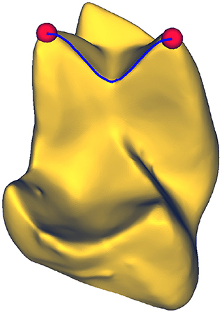
Figure 1. Geodesic path between two points on a surface. A geodesic corresponds to the shortest path connecting any two arbitrary points on a mesh. Molar tooth mesh data from Boyer et al. (2011).

Two meshes are equivalent if there is a map between them that preserves the metrics, and therefore the geodesic distances, on them. The degree of deformation induced by a map can thus be measured by calculating the extent to which geodesic distances are altered by the map, captured in the geodesic matrix $G_{{M}}$. The geodesic matrix is constructed by computing all pairwise geodesic distances such that [$G_{{M}}$]_ij contains the geodesic distance between the two vertices i and j on the mesh ${M}$.

A symmetry of a surface is defined as a self-mapping (i.e., automorphism) Ψ of the mesh that leaves the geodesic matrix unchanged, which is formally expressed as Ψ:${M}$→${M}$ such that [$G_{{M}}$]_x,y = [$G_{{M}}$]_{Ψ(x), Ψ(y)} for every x, y ∈ ${M}$.

Finally, a correspondence Φ between two meshes is formally defined as a mapping that assigns each vertex on a first mesh ${{M}}_1$ to each vertex on a second mesh ${{M}}_2$ as Φ:${{M}}_1$ → ${{M}}_2$. A functional mapping T:${{F}}_{{{M}}_1}$ → ${{F}}_{{{M}}_2}$ maps the space of scalar functions on one mesh (${{F}}_{{{M}}_1}$ ) to the scalar functional space on the other (${{F}}_{{{M}}_2}$). As will be extensively discussed through the paper, the functional mapping provides a useful way of representing the correspondence between two meshes. In order to use it, we need a concrete representation in the form of a finite (k × k) correspondence matrix, denoted as C_Φ.

3. μMatch Pipeline

We hereafter detail each step of the μMatch pipeline that automatically retrieves a one-to-one mapping between pairs of biological objects which surfaces are represented as triangular meshes. The considered objects can be of any nature as long as a mapping reasonably exists between them. To provide an intuitive, non-biological toy example of what a reasonable mapping means: while any four-legged animal such as cats and dogs can plausibly be matched onto one another, they cannot not be plausibly matched with a snake. It is worth noting that there is no formal criterion to determine whether two shapes can meaningfully be put in correspondence, nor for evaluating the quality of the resulting correspondence in the absence of a ground truth. The quality of a matching is therefore usually left to qualitative evaluation.

The μMatch pipeline, summarized in Figure 2, is composed of three main modules. It starts with a pre-processing stage in which the meshes are prepared and cleaned and some important quantities are pre-computed. The second step is the matching algorithm itself, which exploits the functional mapping strategy. Finally, the retrieved correspondence map can be further used for shape analysis. μMatch is implemented in Python 3.7 and is available at github.com/uhlmanngroup/muMatch. In addition to the code itself, we also provide sample data and a script exemplifying the use of the pipeline. For ease of use, all tunable parameters involved in μMatch are gathered in a .yml file along with a description of their meaning and range.

FIGURE 2

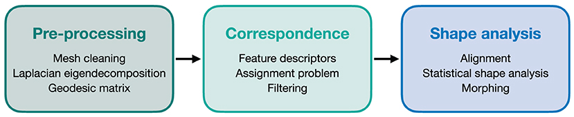
Figure 2. Overview of μMatch. The pipeline, composed of three main steps, automatically retrieves a dense correspondence map between two arbitrary surfaces of biological objects represented as triangular meshes. Individual substeps are listed in each of the boxes.

3.1. Pre-processing

To make them amenable to processing with μMatch, the input objects must satisfy a number of technical requirements. First, each object's surface must be represented in the form of a triangular mesh. These meshes must additionally be both connected and manifold. Being connected implies that, given any two vertices in the mesh, it is possible to find a path consisting of a subset of the mesh edges (i.e., the sides of the faces) that links the two. The manifold condition imposes that the mesh must represent a physically realizable continuous surface. More specifically, it means that each edge in the mesh should be incident to at most two faces, and that the faces attached to a vertex should form an open disk or half-disk around the vertex. An example of non-manifold mesh may involve two parts that are connected by a single vertex, or the presence of an internal face. These different notions are illustrated in Figure 3.

FIGURE 3

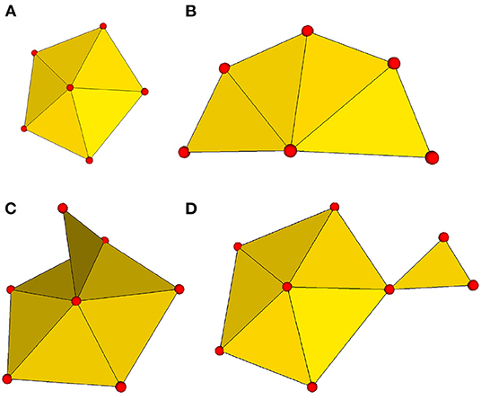
Figure 3. Connectivity and manifold properties. Connectivity attributes expected in a manifold mesh: (A) internal vertex with a full loop of surrounding faces; (B) boundary vertex with a partial loop of surrounding faces. Two examples of non-manifold connectivity: (C) sub-meshes connected by only a single vertex; (D) a single edge shared by more than two triangular faces.

In addition, the matching process assumes that the correspondence map is a bijection, meaning that it defines a way to match ${{M}}_1$ to ${{M}}_2$ as much as a way to match ${{M}}_2$ to ${{M}}_1$. It is therefore crucial that the pairs of meshes have the same coverage, which implies that for each point in ${{M}}_1$, a corresponding point exists in ${{M}}_2$ and vice versa. Finally, it is important for all meshes in the collection to be constructed by sampling as uniformly as possible the object's surface. This translates to vertices in the mesh being equally spaced on each surface, or equivalently to triangular faces having a constant area. μMatch makes use of a number of geometric quantities associated with each mesh, including the geodesic matrix and the Laplace-Beltrami eigen-decomposition introduced in Section 2.2, that may be adversely affected by a non-uniform sampling.

In μMatch, input meshes are cleaned using PyMeshFix 0.14.1 (Attene, 2010), which offers built-in functionalities to remove common errors in triangular meshes, including degenerate and intersecting faces. As a result, output meshes are manifold and watertight with a single connected component. Meshes are subsequently resampled to a user-defined number of vertices N that is smaller or equal than the total number of vertices in the smallest of the input meshes. Importantly, this resampling step processes all meshes to have the same number of vertices regardless of the original number of vertices they were composed of, relieving users from having to handle this constraint. The value of N should be chosen so as to aim at having fine enough meshes to capture important shape features, while limiting the number of vertices to what is necessary in order to avoid overburdening the matching process later.

A final preprocessing step in μMatch, consists of calculating the geodesic matrix of each input mesh using Lib-igl (Jacobson and Panozzo, 2018). Although Lib-igl implements the fast exact geodesic algorithm (Mitchell et al., 1985), it is still computationally demanding with a run-time of O(N²logN) and memory requirement of O(N²), with N the number of vertices in the mesh. For the sake of computational efficiency, we therefore provide a custom data preparation script that precomputes the geodesic matrices for the whole collection of objects and save them to disk prior to the correspondence pipeline.

3.2. Correspondence

The core of μMatch is a landmark-free dense correspondence algorithm adapted from Ovsjanikov et al. (2012), Litany et al. (2017), and Halimi et al. (2019). The correspondence matrix, describing the final mapping, is built from a collection of feature descriptors and refined through filtering steps. The overall workflow is summarized in Figure 4.

FIGURE 4

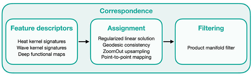
Figure 4. Overview of μMatch's correspondence workflow. The main elements involved in each steps are listed in the corresponding boxes.

3.2.1. Feature Descriptors

Surface matching begins with the calculation of point-wise feature descriptors, referred to as signature functions. Signature functions describe the intrinsic geometry of an object and will therefore return similar values at geometrically similar points on each mesh to be matched. A number of such descriptors have been developed and proposed for the specific purpose of shape correspondence. The first and perhaps most intuitive one is the Gaussian curvature of the mesh, defined as the product of the two principal curvatures, calculated at different scales. More sophisticated techniques include the heat kernel signature (HKS) (Sun et al., 2009), based on solutions of the classical heat equation ∂_tT = ΔT, where Δ is the Laplace-Beltrami operator and T a temperature. The rough idea behind the HKS is to express the remaining temperature after some time t for an initial “heat impulse” fully concentrated at a given point of the mesh. The HKS can be computed for multiple values of t at each point on a mesh to generate a collection of feature descriptors. In practice, the HKS can be calculated efficiently as

$\begin{array}{ll}{h}_t(x)={\displaystyle \sum _{n=0}^N}{e}^{-{\lambda }_{n}t}{\varphi }_n{(x)}^2,& (3)\end{array}$

where {λ_i, ϕ_i} are the pairs of eigenvalues and eigenvectors of the Laplace-Beltrami operator (calculated with Lib-igl in μMatch).

The wave kernel signature (WKS) (Aubry et al., 2011) is closely related to the HKS but instead uses the Schrödinger wave equation (i∂_t + Δ)ψ = 0, which ordinarily governs the dynamics of particles in quantum mechanics. Unlike HKS, WKS assume an approximate particle energy and then determines the long time (i.e., t → ∞) averaged probability distribution for finding the particle in a particular location on the surface. Sampling these distributions for different values of particle energy once again produces a collection of feature descriptors at each point on the mesh. For $f_{ϵ}(E)=\text{exp}(-0.5{(ϵ-\mathrm{\text{log}}(E))}^2/{\sigma }^2)$, where ϵ is the particle energy and σ a scale factor set by the difference between the eigenvalues, it can be shown that the WKS is obtained as

$\begin{array}{ll}{s}_{ϵ}(x)={\displaystyle \sum _{n=0}^N}{f}_{ϵ}{({\lambda }_n)}^2{\varphi }_n{(x)}^2.& (4)\end{array}$

Examples of several HKS and WKS, exhibiting these descriptors' ability to capture geometrically similar features across comparable objects, are illustrated in Figure 5.

FIGURE 5

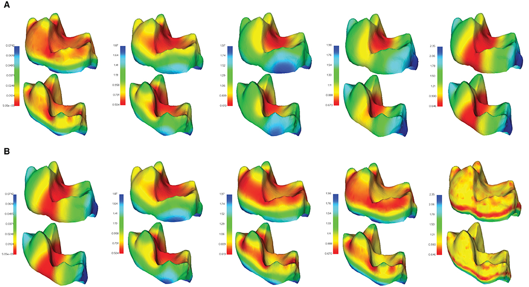
Figure 5. Feature descriptors computed in μMatch. A subset of the descriptors computed from the eigen-decomposition of the Laplacian operator are shown in two different meshes of the TEETH dataset: (A) heat kernel signatures (HKS) for different values of t; (B) wave kernel signatures (WKS) for different values of ϵ. Both types of descriptors can be observed to behave similarly in corresponding areas of the two meshes. Molar teeth mesh data from Boyer et al. (2011).

In order to obtain robust and quickly-computed feature descriptors for use on biological objects exhibiting potentially subtle shape features, μMatch combines HKS and WKS. In practice these quantities are calculated using only the eigenvalues and eigenvectors of the Laplace-Beltrami operator as input, together with the number of functions desired. The total number of extracted HKS and WKS signature functions must be greater or equal as the dimension of the functional space, which corresponds to the size of the correspondence matrix to extract. This parameter can be freely adjusted in μMatch and is set to 100 by default.

A final step in the computation of signature functions consists of passing them through a neural network to improve their overall quality in a process called deep functional maps. Following Halimi et al. (2019), μMatch implements a 7-layer ResNet, which is trained in an unsupervised fashion. Each layer acts on the signature functions by first taking weighted linear combinations of the different signature functions and then passing the result through a non-linear activation function (ReLU). The weights in the linear combination are adjustable parameters that are tuned during the training process such that the output signature functions span the functional space better and therefore produce correspondence maps with lower distortion. Note that while the loss is formulated on the geodesic distance, the neural network is however constrained by the input signature functions. Minimizing the geodesic distance between the two inputs therefore amounts to minimizing distortion subject to aligning the signature functions. As such, the optimization is carried out on intrinsic shape properties (as captured by the signature functions) and not on the geodesic matrix itself. In order to train the network, a subset of the collection of objects to be put in correspondence must serve as training set. As ever, the size of the training set is a trade-off between the ability of the trained network to effectively generalize and the training time, and there is no universal rule to determine how many objects should be included for training. In practice, however, all objects may be used whenever the collection is small. For collections composed of more than a hundred of meshes, a representative subset can be chosen as the training set to speed up computations. We recall that preparing the training set does not require any manual annotation since the network is trained in an unsupervised manner. For each mesh in the training set, the geodesic matrix, the Laplace-Beltrami eigenvectors, an array area encoding the area around each vertex, and the feature descriptors of each mesh are precomputed and saved to a single TensorFlow .tfrecords file for fast data access.

3.2.2. Assignment Problem

The correspondence matching algorithm used in μMatch is based on a method known as functional mapping (Ovsjanikov et al., 2012, 2016) and entirely relies on the computed feature descriptors. The core principle of functional maps is that any mapping between two surfaces induces a corresponding linear mapping between their functional spaces. Formally, this can be demonstrated as follows. Assuming that two surfaces ${{M}}_1$ and ${{M}}_2$ are put in correspondence by a smooth mapping Φ:${{M}}_1$ → ${{M}}_2$, one can define a space of scalar functions on the surface ${{M}}_{\nu }$ as ${{F}}_{{{M}}_{\nu }}$ = {f:${{M}}_{\nu }$ → ℝ} for ν = 1, 2. These spaces can be shown to be infinite dimensional linear vector spaces and the smooth mapping Φ thus induces a linear map T_Φ:${{F}}_{{{M}}_1}$ → ${{F}}_{{{M}}_2}$ through $T_{\Phi }(f)=f\circ {\Phi }^{-1}$, called functional mapping. The linear map T_Φ can be represented as a finite correspondence matrix C_Φ by choosing a (finite) set of k basis functions on the vector spaces ${{F}}_{{{M}}_1}$ and ${{F}}_{{{M}}_2}$. The eigenfunctions of the Laplace-Beltrami operator, ${\left\{{\varphi }_i\right\}}_{i=1}^k$, can be shown to form a complete orthogonal basis of each respective functional space (Ovsjanikov et al., 2012) and encode spatial resolution (also referred to as frequency) when ordered according to their eigenvalues, denoted ${\left\{{\lambda }_i\right\}}_{i=1}^k$, making their choice geometrically meaningful. Because only the k first eigenfunctions are selected, they are referred to as the reduced spectral basis.

A correspondence should first and foremost preserve the signature functions. Given a set of n feature descriptors for each mesh, A ∈ ℝ^k×n and B ∈ ℝ^k×n expressed in the reduced spectral basis, this requirement implies that C_ΦA ≃ B. In the case of perfect isometry, the functional mapping can be shown to commute with the Laplace-Beltrami operator such that C_ΦL₁ = L₂C_Φ, with L_ν the Laplace-Beltrami operator expressed in the spectral basis of ${{M}}_{\nu }$, simply corresponding to a diagonal matrix of the eigenvalues. Whilst exact equality is no longer true in the general case, this relation still approximately holds and can be exploited as a regulariser. The correspondence matrix can be retrieved by solving the regularized linear least squares problem

$\begin{array}{ll}{\text{C}}_{\Phi }={\displaystyle \underset{\text{C}}{argmin}}\left|\right|\text{C}\text{A}-\text{B}|{|}^2+||\delta \text{L}\odot \text{C}|{|}^2,& (5)\end{array}$

where ⊙ is the Hadamard product and ${\left[\delta \text{L}\right]}_{ij}={\lambda }_i^{{{M}}_2}-{\lambda }_j^{{{M}}_1}$, with ${\left\{{\lambda }_{\mu }^{{{M}}_{\nu }}\right\}}_{\mu =1}^k$ the eigenvalues of the Laplace-Beltrami operator on ${{M}}_{\nu }$.

In the presence of any intrinsic symmetries in the mesh, a subset of eigenfunctions called the anti-symmetric space are undistinguishable up to a flip of sign. The signature functions therefore do not provide sufficient information to unambiguously determine how this subset of the function space is mapped between the two meshes. This can lead to parts of the object being mapped with different orientations, leaving large tear discontinuities in-between. To solve this, μMatch implements an additional step after solving (Equation 5) in order to ensure that the resulting map has low distortion. We begin by noting that, much like any scalar function can be decomposed using the spectral basis, so too can any bivariate function, F:${{M}}_{\nu }$ × ${{M}}_{\nu }$ ↦ ℝ, the result being a k×k array. Also, given such a bivariate function F on ${{M}}_1$ and a mapping Φ:${{M}}_1$ ↦ ${{M}}_2$, Φ maps F to a bivariate function F_Φ on ${{M}}_2$, defined by $F_{\Phi }(·,·)=F({\Phi }^{-1}(·),{\Phi }^{-1}(·))$. When expressed in the spectral basis with the correspondence matrix, it reduces to the matrix product $F_{\Phi }=C_{\Phi }F{C}_{\Phi }^T$. The class of bivariate functions that is particularly interesting for the purpose of shape correspondence is the geodesic matrix and functions derived from it. In μMatch, we don't consider the geodesic matrix directly, but rather its Gaussian at several scales σ, defined as ${\text{K}}_{\sigma }^{{{M}}_{\nu }}=exp(-{\text{G}}_{{{M}}_{\nu }}^2/2{\sigma }^2)$, which better encodes neighborhood information. Thus, we expect

$\begin{array}{ll}{C}_{\Phi }{K}_{\sigma }^{{{M}}_1}{C}_{\Phi }^T\simeq K_{\sigma }^{{{M}}_2}.& (6)\end{array}$

The ${\text{K}}_{\sigma }^{{{M}}_{\nu }}$ matrices contain off-diagonal entries that provide information on how different eigenfunctions should relate to one-another, including for the anti-symmetric ones that are not captured by the signature functions. In μMatch, a few fixed values of σ are chosen corresponding to σ ∈ [0.25μ($G_{{M}}$), 0.75μ($G_{{M}}$)], where μ($G_{{M}}$) is the mean surface distance defined as

$\begin{array}{ll}\mu ({\text{G}}_{{M}})=\frac{1}{A_{{M}}^2}{\displaystyle {\int }_{{M}}}{\text{G}}_{{M}}(x,y)d^{2}x{d}^{2}y,& (7)\end{array}$

for a mesh ${M}$ with geodesic matrix $G_{{M}}$ and surface area $A_{{M}}$.

Decreasing the dimension of the spectral basis, captured by the number of basis functions k, increases the stability of the solution of Equation (5). It is therefore better to solve for the correspondence matrix C_Φ at relatively low dimension, generally lying in the range of k = 5 to 12 (μMatch uses k = 8 by default), and then scale up in a process known as ZoomOut Upsampling (Melzi et al., 2019). The downside of working at low dimensions is that much of the off-diagonal information is lost by the omission of higher frequency components from the matrices ${\text{K}}_{\sigma }^{{{M}}_{\nu }}$. Therefore, in order to retain the high frequency information that is required for computing the final k_max-dimensional correspondence matrix, we first compute ${\text{K}}_{\sigma }^{{{M}}_{\nu }}$ matrices at the full dimension k_max, and from this derive the following three reduced (k × k) matrices

$\begin{array}{ll}{\left[{\text{J}}_{{{M}}_{\nu },\sigma }^{(0)}\right]}_{ij}={\left[{\text{K}}_{\sigma }^{{{M}}_{\nu }}\right]}_{ij},& (8)\end{array}$

$\begin{array}{ll}{\left[{\text{J}}_{{{M}}_{\nu },\sigma }^{(1)}\right]}_{ij}={\displaystyle {\sum }_{m=k+1}^{k_{\text{max}}}}{\left[{\text{K}}_{\sigma }^{{{M}}_{\nu }}\right]}_{im}{\left[{\text{K}}_{\sigma }^{{{M}}_{\nu }}\right]}_{mj},& (9)\end{array}$

$\begin{array}{ll}{\left[{\text{J}}_{{{M}}_{\nu },\sigma }^{(2)}\right]}_{ij}={\displaystyle {\sum }_{m,n=k+1}^{k_{\text{max}}}}{\left[{\text{K}}_{\sigma }^{{{M}}_{\nu }}\right]}_{im}{\left[{\text{K}}_{\sigma }^{{{M}}_{\nu }}\right]}_{mn}{\left[{\text{K}}_{\sigma }^{{{M}}_{\nu }}\right]}_{nj}& (10)\end{array}$

for i, j ∈ {1, …, k}. The reduced matrices ${\text{J}}_{{{M}}_{\nu },\sigma }^{(1)}$ and ${\text{J}}_{{{M}}_{\nu },\sigma }^{(2)}$ capture off-diagonal information related to the first k eigenfunctions that would otherwise be lost in the k × k version of ${\text{K}}_{\sigma }^{{{M}}_{\nu }}$ (corresponding to ${\text{J}}_{{{M}}_{\nu },\sigma }^{(0)}$). A k × k correspondence matrix ${\text{C}}_{\Phi }^{(k)}$ can then be obtained by solving the continuous optimisation problem

$\begin{array}{ll}{\text{C}}_{\Phi }^{(k)}={\displaystyle \underset{\text{C}}{argmin}}{\displaystyle \sum _{\sigma }}{\displaystyle \sum _{i=0}^2}{\displaystyle \left|\right|\text{C}{\text{J}}_{{{M}}_1,\sigma }^{(i)}{\text{C}}^T-{\text{J}}_{{{M}}_2,\sigma }^{(i)}|{|}_F^2},& (11)\end{array}$

using the solution of Equation (5) as initial value.

The final, full resolution correspondence matrix is obtained by iteratively increasing k as follows. First, given ${\text{C}}_{\Phi }^{(k)}$, we solve for the point-to-point map by computing a transition matrix Q given as

$\begin{array}{ll}Q=A_{{{M}}_1}{\varphi }_{{{M}}_1}^{(k)}{\left(C_{\Phi }^{(k)}\right)}^T{\left({\varphi }_{{{M}}_2}^{(k)}\right)}^T,& (12)\end{array}$

and a probability matrix P given as

$\begin{array}{ll}{\left[\text{P}\right]}_{ij}={\left[{\text{Q}}^2\right]}_{ij}/{\displaystyle \sum _k}{\left[{\text{Q}}^2\right]}_{ik}.& (13)\end{array}$

The point-to-point mapping Φ is then retrieved by passing P to a linear assignment algorithm (Crouse, 2016), which assigns the indices of vertices of one mesh to those of the other, yielding the maximum probability point-wise correspondence. Conversely, given the point-to-point mapping Φ:${{M}}_1$ ↦ ${{M}}_2$, the associated correspondence matrix of dimension k + 1 can be computed as

$\begin{array}{ll}{C}_{\Phi }^{(k+1)}={\left({\varphi }_{{{M}}_1}^{(k+1)}\right)}^T{A}_{{{M}}_1}\Pi {\varphi }_{{{M}}_2}^{(k+1)},& (14)\end{array}$

where ${\text{A}}_{{{M}}_1}$ is the mesh mass matrix encoding the area around each vertex on ${{M}}_1$, and ${\varphi }_{{{M}}_{\nu }}^{(k)}$ are matrices which columns correspond to the first k Laplace-Beltrami eigenvectors of the mesh ${{M}}_{\nu }$. Finally, Π is the matrix representation of Φ given by

$\begin{array}{ll}{[\Pi ]}_{ij}=\{\begin{array}{ll}1\hfill & \Phi (i)=j\hfill \\ 0\hfill & \text{otherwise}\hfill \end{array}.& (15)\end{array}$

ZoomOut Upsampling thus proceeds to alternate between solving for Π and C_Φ, incrementing the dimension by one each time we solve for C_Φ and repeating until k = k_max, where k_max is the dimension of the reduced spectral basis, chosen such that it provides sufficient resolution for an accurate mapping.

3.2.3. Filtering

The occasional assignment errors and discontinuities that may remain after the correspondence procedure can be filtered out using a technique known as product manifold filter (PMF, Vestner et al., 2017). The PMF aims at producing a bijective and continuous correspondence map by using kernel density estimation. Assuming a noisy and potentially sparse set of I correspondences {_{xi → yi}i = 1, …, I} and a kernel κ (i.e., window function), the function F:${{M}}_1$ × ${{M}}_2$ → ℝ defined as

$\begin{array}{ll}F(x,y)={\displaystyle \sum _{i=1}^I}\kappa (d(x,x_i))\kappa (d(y,y_i)),& (16)\end{array}$

where d is a distance measure (the geodesic distance in our case). The expression (Equation 16) will be maximized when the distance between y and y_i is similar to that between x and x_i for each i = 1, …, I.

A clean mapping Φ:x → y can thus be retrieved when y maximizes (Equation 16), which can be expressed in matrix form as ${\text{F}}_{\sigma }={\text{K}}_{\sigma }^{{{M}}_1}{({\text{K}}_{\sigma }^{{{M}}_2})}^{\text{T}}$, where ${\text{K}}_{\sigma }^{{{M}}_{\nu }}=exp(-{\text{G}}_{{{M}}_{\nu }}^2/2{\sigma }^2)$ and σ = 0.3μ(G) as recommended in Vestner et al. (2017) (see Equation 7). The matrix F is once again passed to a linear assignment algorithm to yield a mapping of vertex indices from one mesh to the other, as done for the probability matrix P in Section 3.2.2, to obtain an updated correspondence.

Ultimately, for a pair of meshes fed into the correspondence pipeline, μMatch returns a correspondence in the form of two matrices, N₁ and N₂, where N₁ are the indices of vertices on the first mesh and N₂ on the second, such that [_N1]n ↦ [_N2]n for each n ∈ N₁. These arrays are saved to disk for reuse in the shape analysis module or outside of μMatch.

3.3. Shape Analysis

3.3.1. Alignment and Statistical Shape Analysis

μMatch allows putting collections of objects in correspondence in order to computationally retrieve the average shape and morphological variations within the collection relying on Procrustes analysis (Kendall, 1989). All objects in the collections are first centered at the origin and scaled to be of unitary root mean square norm. An arbitrary object in the collection is then selected to act as reference, and correspondence maps between this reference and all other objects in the collection are extracted. The final step is to find the best alignment of each object in the collection onto the reference by rotating it. The optimal rotation angle is retrieved by solving the classical orthogonal Procrustes problem (Gower and Dijksterhuis, 2004). Once all objects have been aligned onto the reference, a new reference is obtained by calculating the mean across the entire collection for each corresponding points. The whole process is then repeated, now aligning every shape in the collection to this new reference, and a new updated mean is computed until convergence. The final result is taken as mean shape for the collection.

Relying on the mean of the collection and each object aligned to it, deviations from the mean can be extracted as follows. For each point on the mean shape, μMatch calculates the standard deviation of corresponding points across the entire collection. This results in a scalar function on the reference shape indicating where morphological variations occur and to which extent, and can be visualized as a colormap on the mean shape mesh relying on the vedo visualization library (Musy, 2021). In μMatch, the script implementing this procedure takes as input a directory containing a collection of meshes together with a path to their pre-computed correspondences. The correspondences need only be calculated between the reference shape and each of the other shapes in the collection.

3.3.2. Morphing

Once correspondence between two shapes is established, a continuous morphing between them can be extracted by first aligning the two shapes via translation and rotation (similar to the procedure described in Section 3.3.1, but without scaling), then calculating the geodesic path connecting the two meshes, and sampling shapes along that path. A geodesic being defined as the shortest path connecting any two points in a space, its computation solely requires a notion of distance between points in that space. In Figure 1, we illustrated a geodesic path on a mesh ${M}$, where samples along the path correspond to positions on the mesh. In the case of morphing, the space of interest is instead that of surfaces represented by meshes of fixed connectivity meeting the conditions introduced in Section 3.1: points in the space correspond to the vertex positions and the distance is determined by their connectivity. Samples along the resulting path therefore correspond to meshes. Continuous morphing, going beyond shape analysis of collections of equivalent samples, is of particular interest for image-based modeling, for instance in the context of developmental studies. In Figure 6A, we illustrate as an example the surfaces of a developing mouse limb bud synthetically generated by interpolating between a young and an old limb bud sample. While the older limb bud sample has features (e.g., distributions of surface curvature) for which there is no simple mapping onto the youngest limb bud, the collection of extracted signature functions (Figures 6B,C) manages to capture the local arrangement of these geometrical details with respect to the overall bud shape and allows mapping them to the younger, smoother limb bud in a qualitatively sensible way. As a result, the morphing obtained based on this correspondence produce a visually realistic evolution from one shape onto the other.

FIGURE 6

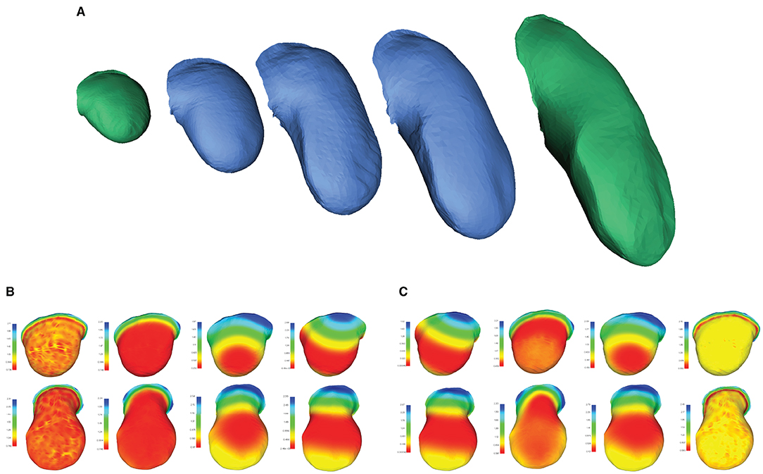
Figure 6. Morphing between two objects in correspondence. (A) Computationally retrieved “growth” of a mouse forelimb obtained by interpolating between two matched meshes of mouse limb buds at early (E10 - E10.5) and late (E11 - E11.5) developmental stages. Meshes in green correspond to samples from the MOUSE_LIMB dataset, while meshes in blue have been synthetically generated through by interpolating along the geodesic path connecting the green meshes. Examples of the set of (B) HKS and (C) WKS used to extract the correspondence. Mesh data from Martínez-Abadías et al. (2018).

Technically, the continuous morphing is obtained following the algorithm proposed in Kilian et al. (2007). Consider a mesh ${{M}}_1$ with vertices v, edges E, and a vector field X describing the deformation of ${{M}}_1$ onto some other mesh ${{M}}_2$. The vector field X is given by difference vectors between the two meshes and thus assumes that a correspondence between ${{M}}_1$ and ${{M}}_2$ has been calculated. Then, the norm ϵ, defined as

$\begin{array}{ll}ϵ(\text{X})={\displaystyle \sum _{i,j\in E}}{\langle {\text{X}}_i-{\text{X}}_j,v_i-v_j\rangle }^2,& (17)\end{array}$

measures the deformation between the two meshes. In order to generate a sequence of meshes morphing the meshes onto one another, the quantity (Equation 17) is minimized through a multi-scale continuous optimisation procedure, starting with low mesh resolution and few intermediate steps and sequentially increasing both. The final geodesic path consists of a set of intermediate meshes that reflects the continuous deformation of one surface onto the other.

4. Experiments

4.1. Quantitative Validation

In order to quantitatively validate μMatch, we use a teeth scan dataset originally introduced by Boyer et al. (2011) and available at www.wisdom.weizmann.ac.il/~ylipman/CPsurfcomp/ and commonly exploited to assess 3D morphometry algorithms. The dataset includes 45 meshes corresponding to mandibular second molars of a variety of prosimian primates and their close non-primate evolutionary relatives, summarized in Table 2. Each specimen is annotated with a set of 16 manually-determined landmarks placed by expert morphometricians that can be used as ground-truth to assess the quality of an automatically-retrieved correspondence. Although this dataset is composed of objects toward the macroscale of the spectrum, it is one of the rare available resources of biological objects for which a ground truth sparse correspondence is available and is as such an excellent candidate for benchmarking. Performance assessment is then carried out following the Princeton benchmark protocol (Shilane et al., 2004; Kim et al., 2011) by computing the mean geodesic error (GE) expressed as

$\begin{array}{ll}\text{GE}=\frac{1}{A_{{{M}}_2}^{1/2}}{\displaystyle \sum _{i=1}^{16}}{\text{G}}_{{{M}}_2}(\Phi (l_i^1),l_i^2),& (18)\end{array}$

where ${\left\{l_i^1\right\}}_{i=1}^{16}$ and ${\left\{l_i^2\right\}}_{i=1}^{16}$ are the ground-truth landmarks on ${{M}}_1$ and ${{M}}_2$, respectively, Φ is the point-to-point mapping, and $G_{{{M}}_2}$ and $A_{{{M}}_2}$ are the geodesic matrix and the surface area of the mesh ${{M}}_2$, respectively. The GE therefore measures how well the main features of the objects have been mapped, regardless of the amount of deformation there may be elsewhere on the surface.

Several processing steps of the μMatch correspondence module (Figure 4), namely the deep functional maps and product manifold filter, aim at improving the final correspondence but are not strictly necessary. While we do recommend including them whenever possible, these steps do increase computation time and the extent of the improvement they will bring cannot be predicted in general for any arbitrary dataset. To provide users with an example of the cost and gains involved, we have quantified the quality of the retrieved correspondence in different settings, by enabling and disabling the deep functional maps and product manifold filter in the μMatch pipeline. In Table 1, we report the average GE between ground-truth landmarks and correspondence points obtained automatically with μMatch for the whole dataset. We also indicate the average runtime to establish correspondence in any given pair. A breakdown of the average GE by species and the cumulative error curves are provided in Figure 7A and Table 2, respectively. We observe the respective merits of the deep functional maps and product manifold filter to be as follows. The deep functional maps improve the signature functions but do not impose smoothness in the final correspondence, resulting in large GE variance. While the correspondence runtime is not affected by deep functional maps since the network is trained during preprocessing, a significant extra amount of compute (~3 h for this dataset) is required ahead of the matching itself, impacting the total duration of the pipeline. In contrast, the product manifold filter ensures that the final correspondence is smooth and does not feature major tears or discontinuities, resulting in small GE variance. It is limited by the correspondence quality that can be obtained from the original signature functions alone and doubles the runtime per pair, but as a trade-off requires no prior computation or training. The combination of the two yields the best results, as it allows obtaining a smooth correspondence from improved signature functions. The cost is however a high runtime per pair for the correspondence itself, and the necessity to go through an expensive training stage during preprocessing.

TABLE 1

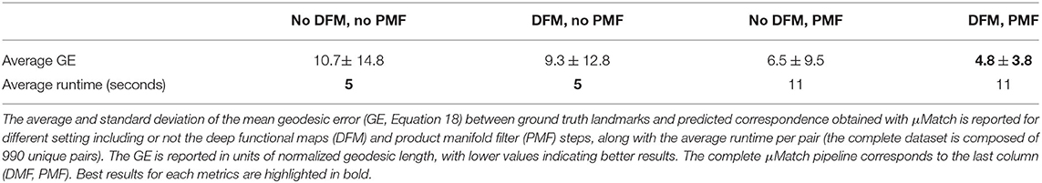
Table 1. Summary of results on the TEETH dataset.

FIGURE 7

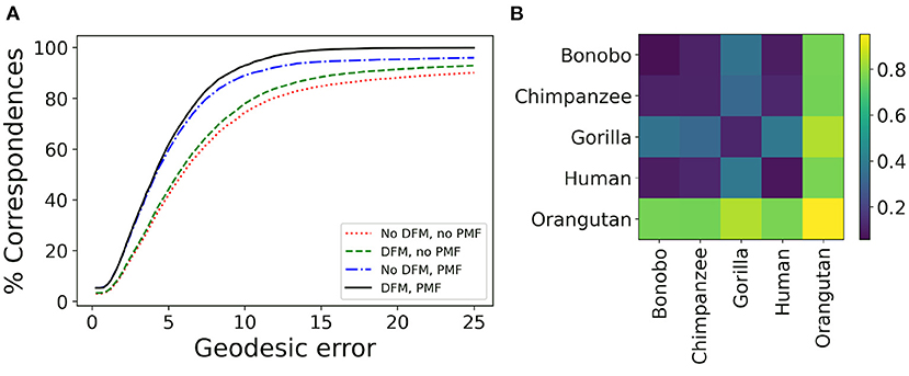
Figure 7. Validation of μMatch. (A) Cumulative geodesic error curve, reporting the proportion of predicted correspondence with an error (Equation 18) smaller than a variable threshold, for different setting including or not the deep functional maps (DFM) and product manifold filter (PMF) steps. The complete μMatch pipeline corresponds to the solid black curve (DMF, PMF). (B) Matrix of average geodesic distance (Equation 19) between species based on the correspondences obtained with the full μMatch pipeline.

TABLE 2

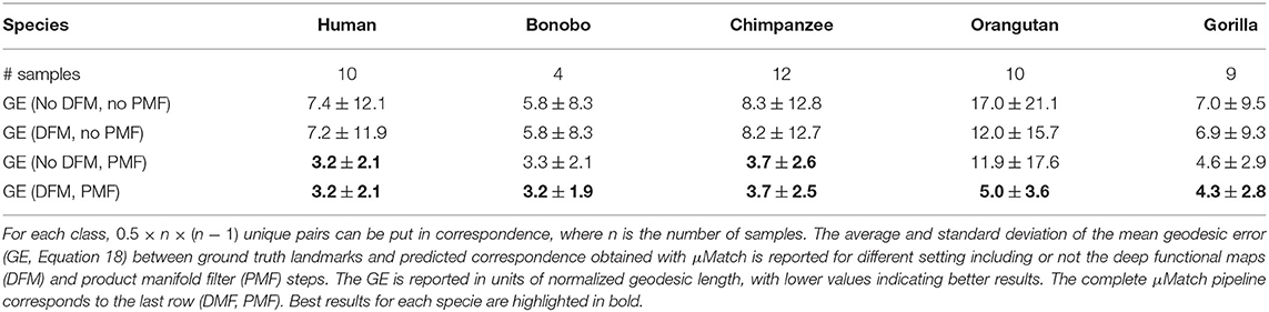
Table 2. Per-specie breakdown of results on the TEETH dataset.

Once correspondence has been established between all meshes in the collection, we carry out a further sanity check by reporting the geodesic distance, or deformation, given by

$\begin{array}{ll}\delta {\text{G}}_{{{M}}_1{{M}}_2}={\displaystyle \sum _{i,j}}{\displaystyle |{\left[{\text{G}}_{{{M}}_1}\right]}_{i,j\in E}-{\left[{\text{G}}_{{{M}}_2}\right]}_{\Phi (i),\Phi (j)}|},& (19)\end{array}$

where E is the set of edges of the meshes ${{M}}_1$ and ${{M}}_2$, and observing how it compares between the different species present in the dataset. We hypothesize that samples from different species will exhibit more shape deviations than individuals from the same species, and investigate whether this can be observed in the geodesic distances retrieved after correspondence established by μMatch. The quantity (Equation 19) is calculated between all pairs in the collection, producing a n × n matrix δG, with n the number of meshes in the collection. Each sub-blocks of the matrix corresponding to the different species can be averaged to produce a reduced distance matrix, depicted in Figure 7B for the full μMatch pipeline (with deep functional maps and product manifold filter). The geodesic distances between species match what would be expected from their phylogeny: molar surfaces of chimpanzees and bonobos are highly similar, and also closely resemble human teeth, while gorilla and orangutan molars are observed to be morphologically more dissimilar. In addition to their differences with other species, samples from the orangutan class appear to be extremely diverse, resulting in a large intra-class distance. This experiment provides a sanity check assessing the validity of the algorithms implemented in the μMatch pipeline. We orient the reader interested in a comparative assessment of the relative performance of the selected correspondence algorithms against published alternatives to the original works introducing functional mapping (Ovsjanikov et al., 2012, 2016).

4.2. Case Study: Joint Shape Analysis of Embryonic Limbs and Dusp6 Gene Expression Patterns

In our previous study (Martínez-Abadías et al., 2018), we performed geometric morphogenesis on a mouse model of Apert syndrome, in which the Fgfr2 gene contains a mutation which models the human syndrome. The goal was to explore whether shape analysis of a gene expression pattern could suggest the molecular basis of the phenotype. In addition to analyzing the developing anatomical changes in the limb, we also analyzed the 3D expression pattern of Dusp6, a gene whose expression reflects the activity of FGF signaling. This allowed subtle alterations in the gene expression pattern to be detected before the anatomical phenotype was apparent, thus strengthening the idea that altered FGF signaling is directly responsible for the phenotype. That previous analysis however depended on manual annotation of 3D landmarks on the data, a process which was very labor-intensive and taking many weeks to achieve. Here, we demonstrate that μMatch can be used to automate this process, jointly quantify the evolution of the shape of embryonic limb and gene expression pattern over developmental time without human bias and achieving similar results in a fraction of the time. We have chosen to reproduce the results of this study to illustrate the use of μMatch on real biological data containing objects that differ in size, orientation, and shape, and exhibit a mixture of inter-group and intra-group variations of morphology.

The dataset we refer to as MOUSE_LIMB, publicly available at dx.doi.org/10.5061/dryad.8h646s0, contains meshes extracted from real optical projection tomography scans (Sharpe et al., 2002) of the limbs and of the Dusp6 gene expression domains of Apert syndrome (Fgfr2 mutants) mouse embryos and unaffected littermates ranging from E10 to E11.5, where EN stands for N days after conception. Extracting these meshes requires the raw image data to be first segmented, a step that can be carried out by different methods. We refer readers interested in the details of the segmentation process to the original study (Martínez-Abadías et al., 2018). The meshes are grouped into forelimbs and hind limbs of early (~E10), mid (~E10.5 to ~E11) and late (~E11.5) developmental periods, according to Table 3. To process these data, we set the number of vertices N to be 2000, and use default μMatch values, namely a functional space dimension of k = 100, and 100 computed heat kernel and wave kernel signatures.

TABLE 3

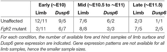
Table 3. Summary of the MOUSE_LIMB dataset.

For each age and genetic background group, a template shape is chosen at random and used to initiate correspondences with the remaining samples. From the mesh correspondences obtained with μMatch, a Procrustes alignment of the limbs surfaces is obtained following the procedure described in Section 3.3.1, yielding an average limb with an associated measure of variance at each vertex. Once limb surfaces are matched, the correspondence can be further used to map internal processes between them, allowing in particular to compare Dusp6 gene expression data available for some of the limbs. The parameters obtained from the limb alignment can then be used to do a rigid registration of the gene expression patterns. This is then further refined by iterative closest point alignment (Besl and McKay, 1992; Chen and Medioni, 1992) and thin plate spline (TPS) deformation to finely warp the objects onto one another (Duchon, 1977). To implement the TPS deformation, the surfaces are first sub-sampled to obtain M control points ${\left\{c_m\right\}}_{m=1}^M$ and the warping is obtained as

$\begin{array}{ll}\delta (x)={\displaystyle \sum _{m=1}^M}{\omega }_m\psi (\left|\right|x-c_m\left|\right|),& (20)\end{array}$

where ψ(r) = r²log(r) is the thin plate spline kernel. The coefficients ${\left\{{\omega }_m\right\}}_{m=1}^M$ are found by solving for Aω = v, where [A]_ij = ψ(||c_i−c_j||)∀i, j = 1, …, M and [v]_m is the difference vector between the source and target surface at the control points m = 1, …, M. Once the objects have been warped onto one another in this manner, a simple nearest neighbors search is used to obtain a correspondence and the shape analysis procedure described in Section 3.3.1 can be carried out again for the gene expression data. The resulting average limbs and gene expression patterns, color-coded according to local variance, are shown in Figure 8. Following Martínez-Abadías et al. (2018), we display results for hind limbs of the early and mid-early stages, and fore limbs of the mid-late and late stages.

FIGURE 8

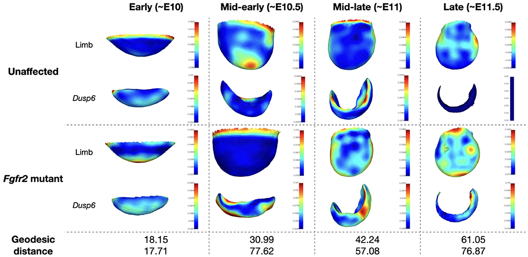
Figure 8. Average limb and Dusp6 gene expression across the MOUSE_LIMB dataset. The averaged surfaces are color-coded according to the local variance (see colorbars). The geodesic distance between the average shape of the unaffected specimen and Fgfr2 mutant is also reported for the limb and Dusp6 gene expression pattern.

In Martínez-Abadías et al. (2018), the limb buds of Fgfr2 mutants from the late period (~E11.5) were observed to separate from those of unaffected littermates. During the mid-early (~E10.5) and early (~E10) periods, the limbs of Fgfr2 mutant mice were however undistinguishable from those of unaffected specimen. Significant difference in Dusp6 gene expression pattern was observed between Fgfr2 mutant animals and their unaffected littermates for all groups except for the early time period. We recover the same results using μMatch, as illustrated in Figure 9, demonstrating the validity of the automatically retrieved correspondence. The difference in shapes was originally quantified by Procrustes analysis relying on sparse set of semi-landmarks along the most distal edge and on the dorsal and ventral sides of the limb (Martínez-Abadías et al., 2018). In contrast, our approach solves for a dense correspondence, taking into account the entire object's surface. The major advantage of μMicro is that it is entirely landmark-free and fully automated. Once limb surfaces are put in correspondence, their geodesic distance can be used to further quantify the extent of their morphological difference, and the recovered matching used to also align their corresponding gene expression. As such, provided that gene expression patterns have been acquired so as to be appropriately registered inside the limb, comparing the shape of gene expression patterns does neither require artificial landmarking nor a separate correspondence map: they instead get aligned based on their “container.” These results demonstrate that μMatch can reliably be used on real bioimage data, which may be noisy, in which samples may exhibit too large variations in their morphology or orientation to rely on volume-based alignment, and which may involve extracted meshes of different numbers of vertices.

FIGURE 9

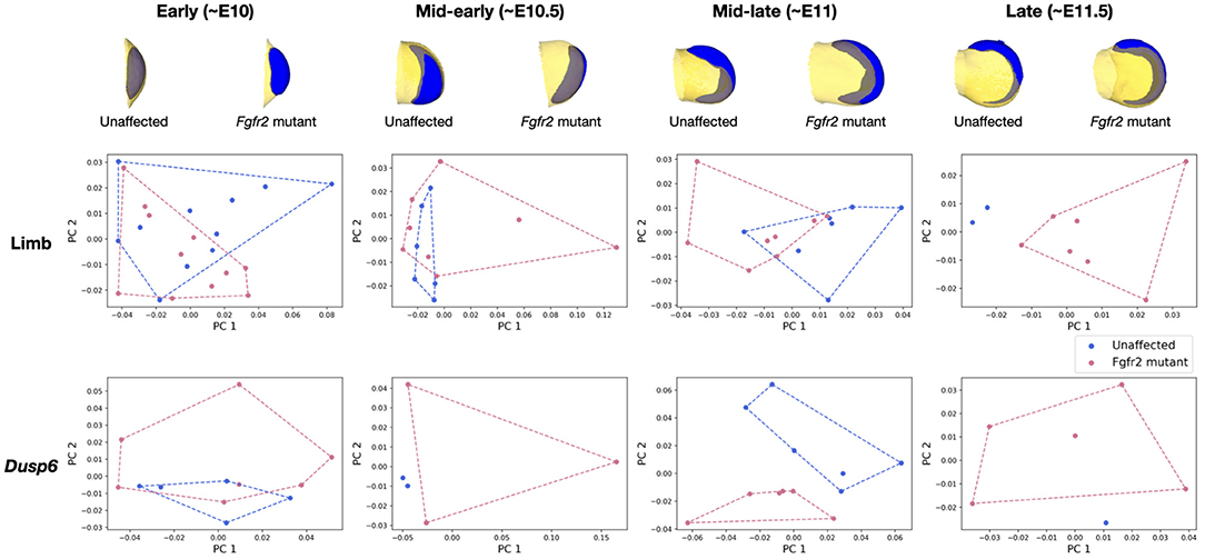
Figure 9. Analysis of the MOUSE_LIMB dataset based on geodesic distances of aligned objects. Vertex-wise deviations from the average shape are concatenated for each mesh in the collection, and reduced by principal component analysis. The resulting two largest principal components are plotted for each sample to quantify the morphological difference between the limbs and Dusp6 gene expression patterns of Fgfr2 mutants and unaffected littermates. The average limb (in yellow) and Dusp6 gene expression pattern (in blue) for each group is displayed on top.

5. Discussion and Conclusions

We developed μMatch, an automated 3D shape correspondence pipeline tailored to biological objects that are difficult or impossible to landmark. The core element of the pipeline is the correspondence algorithm, which is based on functional mapping. As such, μMatch relies entirely on automatically-extracted signature functions that capture the local geometry of the object's surface to retrieve an optimal matching. In addition to the correspondence algoritm itself, μMatch includes scripts to facilitate the whole workflow, from data pre-processing (including mesh cleaning and pre-computation of important quantities to speed up the correspondence process) to basic shape analysis (including Procrustes analysis and morphing). Since the input data format required by μMatch, namely triangular meshes, is very generic, the pipeline can be used for a broad range of objects. While μMatch has no hard limit on the input mesh size, larger meshes will result in more computationally demanding operations and therefore affect execution time. In our experiments, considered meshes were composed of 2,000 to 3,000 vertices (corresponding to 4,000 to 6,000 faces). For much larger meshes, we recommend to establish a first correspondence at a lower resolution (i.e., on decimated meshes) and then extending it to the full sized meshes. As a reference runtime for standard laptops, establishing correspondence between two meshes of 2,000 vertices took approximately 17 s on a laptop with 16Gb of RAM, an Intel Core i7 8th Generation CPU (8 cores), and an Intel Corporation UHD Graphics 620 (rev 07) GPU. μMatch, is implemented in Python and is freely available on GitHub under BSD-3 Clause license.

We quantitatively validated μMatch relying on the TEETH benchmark dataset (Boyer et al., 2011) for which ground truth correspondence is available. Then, we explored the use of μMatch to automate the analysis of a dataset of optical projection tomography scans of mouse limbs (MOUSE_LIMB dataset, Martínez-Abadías et al., 2018) and demonstrated that our pipeline allows retrieving published results. This dataset also includes gene expression patterns which morphologies had originally been studied relying on landmarking. We demonstrated that the limb surface correspondence obtained with μMatch can be used to align the corresponding gene expression patterns without the need for any landmarks, and subsequently characterize their morphological differences. Although involving rather small sample sizes, this experiment is a proof-of-principle that the alignments provided by μMatch can be used to compare the spatial morphology of processes that are internal to the surfaces being matched. Beyond allowing to reproduce and automate morphometry from data at the mesoscopic scale, we hope that μMatch will make it possible to investigate new shape-related questions at the cellular or subcellular scale. Being able to reliably put soft-tissue objects without landmarks in correspondence and use their alignment to register internal processes is a first step toward atlas-free registration, which would be useful in many biological studies involving for instance spatial transcriptomics data.

In addition to enabling the quantitative study of collection of equivalent 3D shapes, dense correspondence maps also allow for continuous morphing between meshes. An exciting future direction of this work is therefore to explore how μMatch can be used to build spatiotemporal models of deforming objects. In a biological context, for instance during development or morphogenesis, complexity will almost always significantly increase over time, resulting in possibly challenging correspondence problems between younger, morphologically simpler surfaces and older ones exhibiting more complex shapes. Because correspondence is an essential first step toward mining 3D surface data extracted from bioimages, we hope that μMatch will help enable new avenues in computational morphometry and modeling for biology and lower the entry cost for life scientists intending to rely on statistical shape analysis to explore their data.

Data Availability Statement

Publicly available datasets were analyzed in this study. This data can be found here: www.wisdom.weizmann.ac.il/~ylipman/CPsurfcomp/; dx.doi.org/10.5061/dryad.8h646s0.

Author Contributions

JK and VU contributed to the conception and design of the work, implemented the methods, carried out the experiments, and wrote the first draft of the manuscript. GD, NM-A, and JS prepared the mouse embryo limb dataset and contributed to the experiments. All authors contributed to final manuscript editing, read, and approved the submitted version.

Funding

JK, JS, and VU are supported by EMBL internal funding. NM-A was supported by the European Union Seventh Framework Program (FP7/2007-2013) under grant agreement Marie Curie Fellowship FP7-PEOPLE-2012-IIF 327382 and by the Grup de Recerca Consolidat en Antropologia Biològica (2017 SGR 1630). GD was supported by the ERC Advanced Grant SIMBIONT (670555) and the Spanish Plan Estatal project: LIMBNET-3D PID2019-110868GB-I00.

Conflict of Interest

The authors declare that the research was conducted in the absence of any commercial or financial relationships that could be construed as a potential conflict of interest.

Publisher's Note

All claims expressed in this article are solely those of the authors and do not necessarily represent those of their affiliated organizations, or those of the publisher, the editors and the reviewers. Any product that may be evaluated in this article, or claim that may be made by its manufacturer, is not guaranteed or endorsed by the publisher.

Acknowledgments

JK and VU acknowledge the NVIDIA Corporation for the donation of a Titan V GPU that made this research possible.

References

Attene, M. (2010). A lightweight approach to repairing digitized polygon meshes. Vis. Comput. 26, 1393–1406. doi: 10.1007/s00371-010-0416-3

CrossRef Full Text | Google Scholar

Aubry, M., Schlickewei, U., and Cremers, D. (2011). “The wave kernel signature: a quantum mechanical approach to shape analysis,” in IEEE International Conference on Computer Vision Workshops (Barcelona: IEEE), 1626–1633.

Google Scholar

Belay, B., Koivisto, J., Parraga, J., Koskela, O., Montonen, T., Kellomäki, M., et al. (2021). Optical projection tomography as a quantitative tool for analysis of cell morphology and density in 3d hydrogels. Sci. Rep. 11, 1–10. doi: 10.1038/s41598-021-85996-8

PubMed Abstract | CrossRef Full Text | Google Scholar

Besl, P., and McKay, N. (1992). A method for registration of 3-d shapes. IEEE Trans. Pattern Anal. Mach. Intell. 14, 239–256. doi: 10.1109/34.121791

PubMed Abstract | CrossRef Full Text | Google Scholar

Boehm, B., Rautschka, M., Quintana, L., Raspopovic, J., Jan, ,ˇ Z., and Sharpe, J. (2011). A landmark-free morphometric staging system for the mouse limb bud. Development 138, 1227–1234. doi: 10.1242/dev.057547

PubMed Abstract | CrossRef Full Text | Google Scholar

Bône, A., Louis, M., Martin, B., and Durrleman, S. (2018). “Deformetrica 4: an open-source software for statistical shape analysis,” in International Workshop on Shape in Medical Imaging (Granada), 3–13.

Google Scholar

Bookstein, F. L. (1997). Morphometric Tools for Landmark Data: Geometry and Biology. Cambridge: Cambridge University Press.

Google Scholar

Boyer, D., Lipman, Y., Clair, E., Puente, J., Patel, B., Funkhouser, T., et al. (2011). Algorithms to automatically quantify the geometric similarity of anatomical surfaces. Proc. Natl. Acad. Sci. U.S.A. 108, 18221–18226. doi: 10.1073/pnas.1112822108

PubMed Abstract | CrossRef Full Text | Google Scholar

Brodoehl, S., Gaser, C., Dahnke, R., Witte, O., and Klingner, C. (2020). Surface-based analysis increases the specificity of cortical activation patterns and connectivity results. Sci. Rep. 10, 1–13. doi: 10.1038/s41598-020-62832-z

PubMed Abstract | CrossRef Full Text | Google Scholar

Chen, Y., and Medioni, G. (1992). Object modelling by registration of multiple range images. Image Vis. Comput. 10, 145–155. doi: 10.1016/0262-8856(92)90066-C

CrossRef Full Text | Google Scholar

Crouse, D. (2016). On implementing 2d rectangular assignment algorithms. IEEE Trans. Aerosp Electron. Syst. 52, 1679–1696. doi: 10.1109/TAES.2016.140952

PubMed Abstract | CrossRef Full Text | Google Scholar

Driscoll, M., Welf, E., Jamieson, A., Dean, K., Isogai, T., Fiolka, R., et al. (2019). Robust and automated detection of subcellular morphological motifs in 3d microscopy images. Nat. Methods 16, 1037–1044. doi: 10.1038/s41592-019-0539-z

PubMed Abstract | CrossRef Full Text | Google Scholar

Dryden, I., and Mardia, K. (2016). Statistical Shape Analysis: With Applications in R, Vol. 995. Hoboken, NJ: John Wiley & Sons.

Google Scholar

Duchon, J. (1977). “Splines minimizing rotation-invariant semi-norms in sobolev spaces,” in Constructive Theory of Functions of Several Variables (Oberwolfach), 85–100.

Google Scholar

Finka, L., Luna, S., Brondani, J., Tzimiropoulos, Y., McDonagh, J., Farnworth, M., et al. (2019). Geometric morphometrics for the study of facial expressions in non-human animals, using the domestic cat as an exemplar. Sci. Rep. 9, 1–12. doi: 10.1038/s41598-019-46330-5

PubMed Abstract | CrossRef Full Text | Google Scholar

Gower, J., and Dijksterhuis, G. (2004). Procrustes Problems, Vol. 30. Oxford: Oxford University Press.

Google Scholar

Grocott, T., Thomas, P., and Münsterberg, A. (2016). Atlas toolkit: fast registration of 3d morphological datasets in the absence of landmarks. Sci. Rep. 6, 1–7. doi: 10.1038/srep20732

PubMed Abstract | CrossRef Full Text | Google Scholar

Hahn, M., Nord, C., Franklin, O., Alanentalo, T., Mettävainio, M., Morini, F., et al. (2020). Mesoscopic 3d imaging of pancreatic cancer and langerhans islets based on tissue autofluorescence. Sci. Rep. 10, 1–11. doi: 10.1038/s41598-020-74616-6

PubMed Abstract | CrossRef Full Text | Google Scholar

Halimi, O., Litany, O., Rodola, E., Bronstein, A., and Kimmel, R. (2019). “Unsupervised learning of dense shape correspondence,” in IEEE Conference on Computer Vision and Pattern Recognition (Long Beach, CA: IEEE), 4370–4379.

PubMed Abstract | Google Scholar

Heinrich, L., Bennett, D., Ackerman, D., Park, W., Bogovic, J., Eckstein, N., et al. (2020). Automatic whole cell organelle segmentation in volumetric electron microscopy. bioRxiv. doi: 10.1101/2020.11.14.382143

CrossRef Full Text | Google Scholar

Horstmann, M., Topham, A., Stamm, P., Kruppert, S., Colbourne, J., Tollrian, R., et al. (2018). Scan, extract, wrap, compute a 3d method to analyse morphological shape differences. PeerJ. 6:e4861. doi: 10.7717/peerj.4861

PubMed Abstract | CrossRef Full Text | Google Scholar

Isensee, F., Jaeger, P., Kohl, S., Petersen, J., and Maier-Hein, K. (2021). nnu-net: a self-configuring method for deep learning-based biomedical image segmentation. Nat. Methods 18, 203–211. doi: 10.1038/s41592-020-01008-z

PubMed Abstract | CrossRef Full Text | Google Scholar

Jacobson, A., and Panozzo, D. (2018). Libigl: A Simple C++ Geometry Processing Library. Available online at: https://libigl.github.io/.

Google Scholar

Kalinin, A., Allyn-Feuer, A., Ade, A., Fon, G.-V., Meixner, W., Dilworth, D., et al. (2018). “3d cell nuclear morphology: microscopy imaging dataset and voxel-based morphometry classification results,” in IEEE Conference on Computer Vision and Pattern Recognition Workshops (Salt Lake City, UT: IEEE), 2272–2280.

Google Scholar

Karanovic, T., and Bláha, M. (2019). Taming extreme morphological variability through coupling of molecular phylogeny and quantitative phenotype analysis as a new avenue for taxonomy. Sci. Rep. 9, 1–15. doi: 10.1038/s41598-019-38875-2

PubMed Abstract | CrossRef Full Text | Google Scholar

Kendall, D. (1989). A survey of the statistical theory of shape. Stat. Sci. 4, 87–99. doi: 10.1214/ss/1177012582

CrossRef Full Text | Google Scholar

Kilian, M., Mitra, N., and Pottmann, H. (2007). “Geometric modeling in shape space,” in ACM SIGGRAPH 2007 (San Diego, CA), 64-es.

Google Scholar

Kim, V., Lipman, Y., and Funkhouser, T. (2011). Blended intrinsic maps. ACM Trans. Graph. 30, 1–12. doi: 10.1145/2070781.2024224

PubMed Abstract | CrossRef Full Text | Google Scholar

Klein, S., Staring, M., Murphy, K., Viergever, M., and Pluim, J. (2009). Elastix: a toolbox for intensity-based medical image registration. IEEE Trans. Med. Imaging 29, 196–205. doi: 10.1109/TMI.2009.2035616

PubMed Abstract | CrossRef Full Text | Google Scholar

Klingenberg, C. (2008). Novelty and homology-free morphometrics: what's in a name? Evol. Biol. 35, 186–190. doi: 10.1007/s11692-008-9029-4

CrossRef Full Text | Google Scholar

Koehl, P., and Hass, J. (2015). Landmark-free geometric methods in biological shape analysis. J. R. Soc. Interface 12, 20150795. doi: 10.1098/rsif.2015.0795

PubMed Abstract | CrossRef Full Text | Google Scholar

Laga, H., Kurtek, S., Srivastava, A., and Miklavcic, S. (2014). Landmark-free statistical analysis of the shape of plant leaves. J. Theor. Biol. 363:41–52. doi: 10.1016/j.jtbi.2014.07.036

PubMed Abstract | CrossRef Full Text | Google Scholar

Lipman, Y., and Funkhouser, T. (2009). Möbius voting for surface correspondence. ACM Trans. Graph. 28, 1–12. doi: 10.1145/1531326.1531378

CrossRef Full Text | Google Scholar

Litany, O., Remez, T., Rodol, E., Bronstein, A., and Bronstein, M. (2017). “Deep functional maps: structured prediction for dense shape correspondence,” in IEEE International Conference on Computer Vision (Venice: IEEE), 5659–5667.

Google Scholar

Lorensen, W., and Cline, H. (1987). “Marching cubes: a high resolution 3d surface construction algorithm,” in Proceedings of the 14th Annual Conference on Computer Graphics and Interactive Techniques (Anaheim, CA), 163–169.

Google Scholar

Lucas, A., Ryder, P., Li, B., Cimini, B., Eliceiri, K., and Carpenter, A. (2021). Open-source deep-learning software for bioimage segmentation. Mol. Biol. Cell. 32, 823–829. doi: 10.1091/mbc.E20-10-0660

PubMed Abstract | CrossRef Full Text | Google Scholar

Lucas, M., Kenobi, K., Von Wangenheim, D., Voβ,, U., Swarup, K., De Smet, I., et al. (2013). Lateral root morphogenesis is dependent on the mechanical properties of the overlaying tissues. Proc. Natl. Acad. Sci. U.S.A. 110, 5229–5234. doi: 10.1073/pnas.1210807110

PubMed Abstract | CrossRef Full Text | Google Scholar

Martínez-Abadías, N., Esparza, M., Sjøvold, T., González-José, R., Santos, M., Hernández, M., et al. (2012). Pervasive genetic integration directs the evolution of human skull shape. Evolution 66, 1010–1023. doi: 10.1111/j.1558-5646.2011.01496.x

PubMed Abstract | CrossRef Full Text | Google Scholar

Martínez-Abadías, N., Estivill, R., Tomas, J., Perrine, S., Yoon, M., Robert-Moreno, A., et al. (2018). Quantification of gene expression patterns to reveal the origins of abnormal morphogenesis. Elife 7:e36405. doi: 10.7554/eLife.36405

PubMed Abstract | CrossRef Full Text | Google Scholar

Melzi, S., Ren, J., Rodolà, K. E., Sharma, A., Ovsjanikov, M., and Wonka, P. (2019). ZoomOut: spectral upsampling for efficient shape correspondence. ACM Trans. Graph. 38, 1–14. doi: 10.1145/3355089.3356524

CrossRef Full Text | Google Scholar

Miao, S., Wang, Z., and Liao, R. (2016). A cnn regression approach for real-time 2d/3d registration. IEEE Trans. Med. Imaging 35, 1352–1363. doi: 10.1109/TMI.2016.2521800

PubMed Abstract | CrossRef Full Text | Google Scholar

Mitchell, J., Mount, D., and Papadimitriou, C. (1985). The discrete geodesic problem. SIAM J. Comput. 16, 647–668. doi: 10.1137/0216045

CrossRef Full Text | Google Scholar

Musy, M., Jacquenot, G., Dalmasso, G., Neoglez de Bruin, R., Pollack, A., et al. (2021). vedo, a python module for scientific analysis and visualization of 3D objects and point clouds. Zenodo. doi: 10.5281/zenodo.4287635

CrossRef Full Text | Google Scholar

Ovsjanikov, M., Ben-Chen, M., Solomon, J., Butscher, A., and Guibas, L. (2012). Functional maps: a flexible representation of maps between shapes. ACM Trans. Graph. (Macao) 31, 1–11. doi: 10.1145/2185520.2185526

CrossRef Full Text | Google Scholar

Ovsjanikov, M., Corman, E., Bronstein, M., Rodolà, E., Ben-Chen, M., Guibas, L., et al. (2016). “Computing and processing correspondences with functional maps,” in ACM SIGGRAPH Asia 2016 Courses, 1–60.

Google Scholar

Paul-Gilloteaux, P., Heiligenstein, X., Belle, M., Domart, M.-C., Larijani, B., Collinson, L., et al. (2017). ec-clem: flexible multidimensional registration software for correlative microscopies. Nat. Methods 14, 102–103. doi: 10.1038/nmeth.4170

PubMed Abstract | CrossRef Full Text | Google Scholar

Phillip, J., Han, K.-S., Chen, W.-C., Wirtz, D., and Wu, P.-H. (2021). A robust unsupervised machine-learning method to quantify the morphological heterogeneity of cells and nuclei. Nat. Protoc. 16, 754–774. doi: 10.1038/s41596-020-00432-x

PubMed Abstract | CrossRef Full Text | Google Scholar

Pinkall, U., and Polthier, K. (1993). Computing discrete minimal surfaces and their conjugates. Exp. Math. 2, 15–36. doi: 10.1080/10586458.1993.10504266

CrossRef Full Text | Google Scholar

Preibisch, S., Saalfeld, S., Schindelin, J., and Tomancak, P. (2010). Software for bead-based registration of selective plane illumination microscopy data. Nat. Methods 7, 418–419. doi: 10.1038/nmeth0610-418

PubMed Abstract | CrossRef Full Text | Google Scholar

Ramirez, P., Zammit, J., Vanderpoorten, O., Riche, F., Blé, F.-X., Zhou, X.-H., et al. (2019). Optij: open-source optical projection tomography of large organ samples. Sci. Rep. 9, 1–9. doi: 10.1038/s41598-019-52065-0

PubMed Abstract | CrossRef Full Text | Google Scholar

Rohlf, F., and Slice, D. (1990). Extensions of the procrustes method for the optimal superimposition of landmarks. Syst. Biol. 39, 40–59. doi: 10.2307/2992207

CrossRef Full Text | Google Scholar

Schmidt, P., Born, J., Campen, M., and Kobbelt, L. (2019). Distortion-minimizing injective maps between surfaces. ACM Trans. Graph. 38, 1–15. doi: 10.1145/3355089.3356519

CrossRef Full Text | Google Scholar

Schreiner, J., Asirvatham, A., Praun, E., and Hoppe, H. (2004). “Inter-surface mapping,” in ACM SIGGRAPH 2004 (Los Angeles, CA).

Google Scholar

Sharpe, J., Ahlgren, U., Perry, P., Hill, B., Ross, A., Hecksher-Sørensen, J., et al. (2002). Optical projection tomography as a tool for 3d microscopy and gene expression studies. Science 296, 541–545. doi: 10.1126/science.1068206

PubMed Abstract | CrossRef Full Text | Google Scholar

Shilane, P., Min, P., Kazhdan, M., and Funkhouser, T. (2004). “The princeton shape benchmark,” in Proceedings of the International Conference on Shape Modeling Applications (Genova), 167–178.

Google Scholar

Sorkine, O., and Alexa, M. (2007). “As-rigid-as-possible surface modeling,” in ACM SIGGRAPH 2007 (San Diego, CA), 109–116.

Google Scholar

Srivastava, A., Klassen, E., Joshi, S., and Jermyn, I. (2010). Shape analysis of elastic curves in euclidean spaces. IEEE Trans. Pattern Anal. Mach. Intell. 33, 1415–1428. doi: 10.1109/TPAMI.2010.184

PubMed Abstract | CrossRef Full Text | Google Scholar

Sun, J., Ovsjanikov, M., and Guibas, L. (2009). A concise and provably informative multi-scale signature based on heat diffusion. Comput. Graph. Forum 28, 1383–1392. doi: 10.1111/j.1467-8659.2009.01515.x

CrossRef Full Text | Google Scholar

Toussaint, N., Redhead, Y., Vidal-García, M., Lo Vercio, L., Liu, W., Fisher, E., et al. (2021). A landmark-free morphometrics pipeline for high-resolution phenotyping: application to a mouse model of down syndrome. Development 148, dev188631. doi: 10.1242/dev.188631

PubMed Abstract | CrossRef Full Text | Google Scholar

van der Walt, S., Schönberger, J., Nunez-Iglesias, J., Boulogne, F., Warner, J., Yager, N., et al. (2014). scikit-image: image processing in Python. PeerJ. 2:e453. doi: 10.7717/peerj.453

PubMed Abstract | CrossRef Full Text | Google Scholar

Van Kaick, O., Zhang, H., Hamarneh, G., and Cohen-Or, D. (2011). A survey on shape correspondence. Comput. Graph. Forum 30, 1681–1707. doi: 10.1111/j.1467-8659.2011.01884.x

CrossRef Full Text | Google Scholar

Vestner, M., Litman, R., Rodol, E., Bronstein, A., and Cremers, D. (2017). “Product manifold filter: non-rigid shape correspondence via kernel density estimation in the product space,” in IEEE Conference on Computer Vision and Pattern Recognition (Honolulu, HI: IEEE), 6681–6690.

Google Scholar

Voigt, F., Kirschenbaum, D., Platonova, E., Pagès, S., Campbell, R., Kastli, R., et al. (2019). The mesospim initiative: open-source light-sheet microscopes for imaging cleared tissue. Nat. Methods 16, 1105–1108. doi: 10.1038/s41592-019-0554-0

PubMed Abstract | CrossRef Full Text | Google Scholar

White, J., Ortega-Castrillón, A., Matthews, H., Zaidi, A., Ekrami, O., Snyders, J., et al. (2019). Meshmonk: open-source large-scale intensive 3d phenotyping. Sci. Rep. 9, 1–11. doi: 10.1038/s41598-019-42533-y

PubMed Abstract | CrossRef Full Text | Google Scholar

Windheuser, T., Schlickewei, U., Schmidt, F., and Cremers, D. (2011). “Geometrically consistent elastic matching of 3d shapes: a linear programming solution,” in IEEE International Conference on Computer Vision (Barcelona: IEEE), 2134–2141.

Google Scholar

Yang, X., Kwitt, R., Styner, M., and Niethammer, M. (2017). “Fast predictive multimodal image registration,” in IEEE 14th International Symposium on Biomedical Imaging (Melbourne, VIC: IEEE), 858–862.

PubMed Abstract | Google Scholar

Yeh, Y.-C., Weng, C.-H., Huang, Y.-J., Fu, C.-J., Tsai, T.-T., and Yeh, C.-Y. (2021). Deep learning approach for automatic landmark detection and alignment analysis in whole-spine lateral radiographs. Sci. Rep. 11, 1–15. doi: 10.1038/s41598-021-87141-x

PubMed Abstract | CrossRef Full Text | Google Scholar