The Spatial Leaky Competing Accumulator Model

Introduction

We are able to process incoming sensory information rather quickly and efficiently despite limited processing resources available in the brain and the high energy costs of neuronal computations (Lennie, 2003). Given the need to allocate energy for various task demands, attention is commonly described as a system that can select a subset of available sensory information for further processing. In visual attention, selection is often likened to a moving spotlight across the visual field in order to highlight the regions that are most distinguishable and relevant for the task (Carrasco, 2011). In this model, a relatively small region of the entire visual field can be selected and hence attended at any moment, and would result in a boost of perceptual processing in the selected area. Shifts of attention can be driven by bottom-up or top-down factors. The latter follow the task goal and volitional control, while bottom-up factors are task-independent and are determined by objective physical characteristics of the stimulus (Posner, 1980).

Models of bottom-up attention can be used to predict where humans will look in tasks like free examination of a scene or visual search (with some limitations, as the scope of top-down influence may vary a lot depending on the nature of the stimuli). The algorithms at the heart of these models are often based on the idea that attention can be captured by the physical characteristics of the retinal input. In general, objects most different from their surroundings are considered the most salient. These models are consistent with the feature integration theory of attention in that saliency can be computed pre-attentively for different features (Treisman and Gelade, 1980). At the early pre-attentive stage, elementary perceptual properties (shape, color, brightness et al.) of a stimulus are perceived in parallel and encoded into separate feature maps. The attentive stage is for normalizing and integrating the feature maps into a higher-level representation—a saliency map. This map corresponds to the spatial dimensions of the initial visual field and encodes the overall saliency of that region. The saliency map provides a representation of the visual field, where the most conspicuous locations are emphasized.

There are multiple candidate areas for locus of a saliency map in the brain. Zhaoping et al. argued that neurons of the primary visual area (V1) respond to basic low-level features of the image and constitute a saliency map, basing this assumption on psychophysical tests (Zhaoping and May, 2007) and neuroimaging recordings (Zhang et al., 2012). For Gottlieb (2007), a salience representation of the incoming image in monkeys is best matched by the lateral intraparietal area (LIP) with the most analogous brain area in humans being intraparietal sulcus (IPS) (Van Essen et al., 2001). Some authors argue that the concept of saliency map might be biologically invalid (Fecteau and Munoz, 2006), since top-down modulations interfere with bottom-up visual processing at all intermediate and higher levels of the visual system (such as LIP, FEF, and SC). They suggested a brain representation of the attentional map as a priority rather than a saliency map. A priority map emphasizes that allocating spatial attention is based on both bottom-up saliency and top-down goal-related prioritization of the information (Fecteau and Munoz, 2006; Bisley and Mirpour, 2019).

Although originally focused on bottom-up processing, more recent saliency models have extended the idea to include top-down attention. Feature biasing, for example, has been used to assign weights to feature maps when building a saliency map. This can be implemented through supervised learning (Borji et al., 2012) or with use of eye movements recordings (Zhao and Koch, 2011; also see Itti and Borji, 2013 for a review). Alternatively, spatial biasing could favor certain locations that are important for scene context (Torralba et al., 2006; Peters and Itti, 2007). Another class of models operates on objects rather than feature salience, and requires an object recognition component (see Krasovskaya and MacInnes, 2019 for review). An example is the object-based visual attention model of Sun and Fisher (2003) which includes competition between objects, their grouping and consequent hierarchical attention shifts with use of top-down modulations.

The most interesting examples of saliency models, from a cognitive neuroscience perspective, include a strong theoretical basis along with neurally plausible computational approaches. For example, gaussian pyramids are used to reflect center-surround receptive fields in the primary visual cortex, and also show a good fit to human data for spatial localization of salient stimuli (Merzon et al., 2020). However, according to MIT/Tuebingin Saliency Benchmark (Bylinskii et al., 2018), classical implementations of saliency models are inferior to novel approaches, such as deep neural networks (Kümmerer et al., 2017; Jia and Bruce, 2020) that turn the problem into one of spatial classification. Nevertheless, biological plausibility of saliency models provides good interpretability and theoretical value.

Another advantage of saliency models is that some implementations (e.g., Walther and Koch, 2006) have the capability to predict temporal dynamics of gaze responses. In general, modeling attentional shifts at the computational level can be tested in a variety of ways including their spatial and temporal components. Spatial models predict where we allocate attention, and their performance is often measured with overt attention, i.e., locations of gaze fixations and tested using established metrics like Accuracy Under Curve or AUC-Judd (Judd et al., 2009). Models that include temporal predictions are less common and may predict the order of these eye movements (a scanpath) and/or their latency distribution. Although early salience models were able to predict fixation latencies (Walther and Koch, 2006), the classical saliency model was shown to have serious limitations in simulating the temporal dynamics of human data (Merzon et al., 2020). At the same time, alternative deep learning-based approaches usually focus on the spatial component alone, and very few of these models address the temporal aspect at all.

Other alternatives have been recently introduced that have adapted Bayesian or diffusion techniques to generate fixations in both space and time. For example, Ratcliff (2018) implemented a spatial version of the drift diffusion model. The Spatially Continuous Diffusion Model (SCDM) allowed input from a 2-dimensional plane and predicted decision responses when a location on a planar threshold was reached allowing spatial-temporal prediction from touch or eye movement responses. This model was not tested specifically on salience map input, though the planar input used would likely allow this use case.

Additionally, the model LATEST (Tatler et al., 2017) implements a Bayesian decision process to model each fixation as a stay vs go competition to predict fixation latencies and locations. Temporally, the Bayesian process is shown to be an excellent fit to human fixation latencies. Spatially, the model calculated pixel-wise decisions based in part on maps derived from image salience, but also include a map of semantic importance as defined by human rating. Fixations were planned in parallel over the full image using decision maps (as opposed to salience or priority maps) and tended to choose fixations that landed within the high salience areas (Judd et al., 2012).

Computational saliency models can be conceptualized as sequential modules consisting of processing units likened to neuronal populations. At the first stage basic physical properties of visual stimuli are encoded in feature maps, which are further normalized and aggregated into a single saliency or priority map. While many saliency models stop at these spatial predictions, an additional temporal level of the model might generate shifts of attention in a winner-take-all (WTA) fashion: first, the most salient location is attended, with subsequent fixations steered toward novel locations with an inhibitory mechanism like inhibition of return (Posner, 1980). This allocation of attention to each fixational point at the temporal layer could be implemented via a spiking neuron model (Trappenberg et al., 2001; Adeli et al., 2017). Processing units imitate neuronal populations which build up electrical potential and fire when exceeding a certain threshold.

However, many current saliency models have focused on predicting spatial fixations and not retained the ability to imitate spiking processes and predict temporal information. Although the classical saliency model is able to generate a fixation latency distribution, it does not show a good fit to human data (Merzon et al., 2020). We believe there is a gap in the current literature for an alternative mechanism of fixation selection that works with existing saliency map spatial localization.

One candidate to implement a spatial saliency map is the Leaky competing accumulator (LCA; Usher and McClelland, 2001). The Leaky Competing Accumulator has a two-layered structure: the first layer consists of multiple (usually two) visual input stimuli, and the second computational layer includes a range of neuron-like processing units. Each processing unit corresponds to a single input element. Over time, the processing units accumulate information from the input layer, i.e., gradually increase their values over time. When the value of some unit exceeds a threshold, a decision is made and the corresponding input is considered selected. Thus, human fixation latency is simulated as the amount of time it took the model to decide about the next fixation. In comparison with related accumulator models (Ratcliff et al., 2007; Brown and Heathcote, 2008; Ratcliff and McKoon, 2008), the LCA includes a range of additional parameters: information leakage, recurrent self-excitation, randomness, and lateral inhibition. Each of the parameters is well-justified from a biological point of view, and we briefly describe below the psychophysiological phenomena imitated by the model parameters.

Neural currents can be characterized in terms of their passive decay over time. This decay has exponential properties and results in a partial loss, or leakage of information from visual input (Abbott, 1991). The LCA model implements this decay, which leads to a slower increase in the unit values and also filters out weak stimulations that produce insufficient excitation and vanish with decay over time. A second important mechanism, which counteracts and balances such decay, is recurrent self-excitation. This allows neural units to maintain their activity over time and decrease the rate of information leakage (Amit, 1989). Self-excitation is implemented in the model as bottom-up excitatory input to all accumulator units.

Thirdly, LCA incorporates lateral inhibition as a mechanism for neural competition. Although axonal projections from one brain region to others are overwhelmingly excitatory, within a single brain area there are both excitatory and inhibitory interactions (Chelazzi et al., 1993). Lateral inhibition accounts for each active neuron inhibiting adjacent neurons to it in a lateral direction. In the original LCA, the value of each processing unit is decreased by a sum of all others' values at every time moment. Thus, self-excitation and lateral inhibition balance each other with units multiplied by their own scaled values from the previous time moment and simultaneously decreased by the values of others.

Proposal

We propose a model of allocating attention as a series of spatio-temporal decisions about where to make the next saccade. The suggested model belongs to the family of information accumulators that represent perceptual decision making as a stochastic process that is gradually evolving over time (Smith, 1995; Usher and McClelland, 2001; Brown and Heathcote, 2008; Ratcliff and McKoon, 2008). These models are extremely accurate in reproducing temporal response distributions (MacInnes, 2017) and can also model neural accumulation in areas like the superior colliculus (Ratcliff et al., 2007).

Specifically, our model is based on the Leaky Competing Accumulator (the LCA; Usher and McClelland, 2001) for calculating information accumulation.

Lateral inhibition is a key mechanism allowing multiple inputs to the LCA model (Usher and McClelland, 2001), but one challenge for adopting an accumulator model to simulate a salience map construction is that traditional algorithms most often select between only two abstract alternatives. Practically, neural competition between multiple alternatives can be imitated by feed-forward inhibition with each input unit sending a positive signal to a corresponding accumulator unit and similar negative values to all others (Heuer, 1987). However, with the increasing number of alternatives, all neurons except the most active would receive excess inhibition, drop below zero quickly and hence fail to compete. Thus, accurate modeling becomes challenging. While race models can also be extended to multiple competing alternatives, each random accumulator added shifts the response distribution to an earlier bias (Wolfe and Gray, 2007). Lateral inhibition, however, may allow for accurate modeling of this neuronal competitive interplay. All inputs to processing units would be excitatory, and the value of inhibition would not need to be as drastic as that of feed-forward. The most active accumulator unit could inhibit the others significantly but gradually and would not result in negative activation after the first iteration. However, in the original LCA model, each neuronal unit sends inhibitory signals to all others, which is not entirely biologically plausible, especially as we consider neurons on a spatial salience map.

We suggest an implementation of LCA that uses a saliency map as an input and operates in both temporal and spatial domains, generating fixation coordinates over time. Thus, the leaky competing accumulator becomes a spatial leaky competing accumulator (SLCA). The number of internal processing units corresponds to the size of the input saliency map, and each of these units represent a corresponding neuronal population. Although these salience maps often describe their size in terms of “pixels,” we will only use the term in the abstract sense of a population's receptive field.

We further propose an alternative implementation of lateral inhibition in LCA, so that each neuron-like unit could influence only its immediate neighbors. In this light, a key advantage of our SLCA would be its mechanism of lateral inhibition, allowing the model to simulate the neuronal competition in visual pathways. Each processing unit would accumulate information over time, and only the first unit to achieve a threshold fires at the moment. Neuron-like elements are thus competing for limited brain attention resources, and their competition is driven by a range of physiologically accurate mechanisms.

SLCA Model Architecture

Our model shares the two-layer network structure and the base algorithm for the update of unit values with the original LCA model. Please see the full model architecture on Figure 1.

FIGURE 1

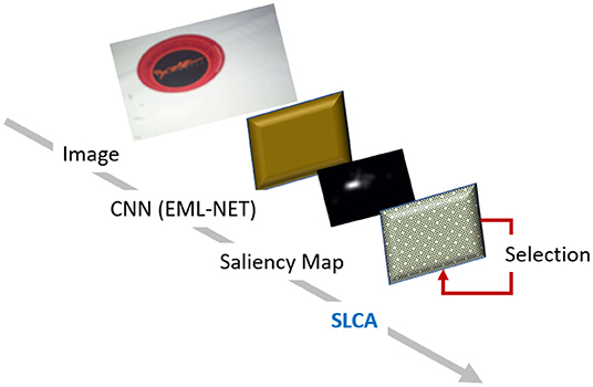
Figure 1. SLCA model architecture. We use EML-Net to produce the salience maps, which are then used as input to our model.

The first layer includes the external input to the model. Our SLCA model does not work directly with image or retinal input, but uses salience/priority map as input. As such, we used an off the shelf implementation of EML-Net to provide the salience maps from the images for our training and testing procedures. The original LCA model operates with several input choice alternatives but without consideration for the spatial proximity of those choices. In our case, a fundamental consideration was that the input would be a two-dimensional salience or priority map, so spatial proximity was added.

The second layer is the same for SLCA and LCA and it consists of accumulator units which are roughly analogous to neural activation clusters processing information about different alternatives. Finally, a winner-take-all selection mechanism was implemented to act iteratively on this layer. Many models use Inhibition of return (IOR) to reduce the likelihood of refixating salient locations but we chose not to implement this mechanism at this time since the previous simple mechanisms implemented may not match the two forms that are proposed to exist (Redden et al., 2021). In terms of processing mechanisms, LCA and our SLCA are quite similar. Much of the description below applies to both models but we highlight where key differences occur.

Accumulator units can be characterized in terms of their input and output values. Input values correspond to the neural population current, i.e., neural activation. The output values stand for population firing rate, which is calculated with use of a linear threshold function. This function can well-approximate relations between the firing rate and the input current (Mason and Larkman, 1990; Jagadeesh et al., 1992). The response is triggered by the unit whose activation first reaches a threshold. Thus, the time required for reaching this criterion value simulates human RT before the next saccade.

Algorithm

The mechanism of information processing in both LCA and our SLCA models is implemented in the dynamic behavior of the units' activations and their continuous interplay. The algorithm describes how values of the accumulator units increase over time until one of them reaches the threshold. The original LCA model used a constant threshold value, however, our temporal predictions largely depend on the input saliency map values and are sensitive to its changes. Models like the original salience map (Itti and Koch, 2000) normalized the conspicuity maps prior to the leaky integrate and fire layer. However, we achieved this result with a dynamic threshold parameter that depends on the input saliency map values, in the Equation (1).

$\begin{array}{ll}T=T_0+m^{*}(S>0.6)& (1)\end{array}$

Here, T stands for the unit activation threshold, which is the sum of two terms. T₀ stands for the default threshold value, which is independent from the saliency map values. S stays for the saliency map values, and m is the special saliency multiplication factor. The larger m is, the more the resulting threshold value depends on the saliency map.

In general, the model tends to behave as a charging capacitor with an exponential approach. The formula for updating unit values in the original LCA model is presented in the Equation (2).

$\begin{array}{ll}d{x}_i={[{\rho }_i-k{x}_i-\beta {\displaystyle \sum _{j\ne i}{x}_j}]}^{*}\frac{dt}{t}+f+ E_i\sqrt{\frac{dt}{t}}& (2)\end{array}$

$\begin{array}{l}{x}_i\to (x_i,0)\\ j\in (0,n)\end{array}$

Here, dx_i describes the change of the i-th accumulator unit activation value for the time interval $\frac{dt}{t}$. This change is driven by the external input ρ_i, the excitatory input x_i and overall inhibition $\beta \sum _{j\ne i}{x}_j$. k stands for the overall net leakage. E_i stands for Gaussian random noise, f–for offset. n is the total number of accumulator units. In order to achieve biological plausibility, an additional restriction is introduced in the model: if the activation value of any accumulator unit has a value lower than 0, it should be immediately truncated to 0.

The external feed-forward input ρ_i is a weighted sum of all inputs of the first layer to the i-th accumulator unit. Greater weight is assigned for the i-th input in comparison with all others. Note that it is possible via simplifying assumption that all of the input units have a zero value before stimuli presentation, and after it these values change in accordance with stimuli saliency values.

The k term stands for the overall net leakage, which is the difference between the recurrent self-excitation and information decay. The corresponding formula is presented in the Equation (3).

$\begin{array}{ll}k=\lambda a& (3)\end{array}$

Here, a is a scaling factor for the recurrent self-excitation, while λ represents information decay, or leakage of activation. They function together as factors for excitatory input, and the resulting k factor represents balance between self-excitation and leakage. With k > 0 the system is stable and tends to zero activation over time, whereas k <0 allows for self-amplifying and hence instability of the system.

The overall inhibition of a unit in the original LCA model depends on the input from the other units. It is represented by a sum of other units' activations multiplied by a scaling term β. Thus, during the accumulation process, each alternative sends inhibiting signals to all others.

The original LCA model uses inputs abstracted in space, such as several choice alternatives. Regardless of the number of inputs, there is no sense of spatial proximity between units. It operates only in the temporal domain, predicting each units' activation over time. In contrast, our proposed Spatial LCA model accounts for data in two dimensions and predicts activation on this map over time. We use a saliency map as an input to the model thus extending the number of choice alternatives up to the number of input units in the saliency map. The second layer of the SLCA model consists of a 2-dimensional array of information accumulation units. These units are likened to neural activation clusters representing a spatial location.

One may consider a simple visual search task, with each location on the saliency map represented by a single node of the input level. The second level of the network includes an equivalent number of units with each corresponding to a certain location. Thus, the external feed-forward input becomes a weighted sum of all inputs of the saliency map to the ij-th accumulator unit. The entire model is a simulation of fixation selection as perceptual decision making over a stimulus picture for each time step.

A spatial implementation, however, raises an important question of the degree to which neighboring neurons can influence the rest of the grid. To this end, we implemented two versions of the algorithm for SLCA values update with the crucial difference being whether the lateral inhibition parameter had global or local. The global version is analogous to the original LCA algorithm, where each accumulator unit is potentially inhibited by all others. We propose an alternative local implementation of lateral inhibition where each unit inhibits only its immediate neighbors. Thus, there are eight inhibited neighbors for all non-borderline units. As for those corresponding to units on the physical border of the saliency map, the number of neighbors to inhibit varies from three to five units. Equation (4) contains the resulting formula for values update.

$\begin{array}{ll}d{x}_i={[{\rho }_i-k{x}_i-\beta {\displaystyle \sum _{j\ne i}{x}_j}]}^{*}\frac{dt}{t}+f+ E_i\sqrt{\frac{dt}{t}}& (4)\end{array}$

$\begin{array}{l}{x}_i\to (x_i,0)\\ j\in (i\pm 1,i\pm w,i\pm w\pm 1)\end{array}$

The Equation (4) shares the parameters dx_i, ρ_i, k, x_i, β, f, E_i, $\frac{dt}{t}$ with the equation (2). Also, a new parameter w is introduced. It stands for the width of the original stimulus image and is used to identify the coordinates of neighboring units, which are further used for calculating the local inhibition.

Materials

Evaluating the model performance was accomplished by comparing it with human data. We used data from a visual foraging task using natural indoor scenes as stimuli. Forty six participants had to search real photos of scenes for multiple instances of either cups or pictures. These images were taken from the LabelMe dataset (Russell et al., 2008), which provides images of indoor and outdoor scenes. Data were collected using an eye tracker EyeLink 1000+, with the sampling rate 1,000 Hz. Fixation detection was set to a velocity threshold of 35 degrees per second. Fixations with RT <100 and >750 ms were dropped as outliers. The dataset size after outliers' exclusion was 55,400 sample fixations. A detailed description of the data collection process was provided in Merzon et al. (2020). The data was collected with ethical approval from the HSE ethics committee and conforms to the protocols listed in the declaration of Helsinki.

All data was divided into a test and training set. The data from 36 randomly chosen participants were used for the optimization procedure, and data from the remaining 10 participants were used for testing. Each participant viewed 23 pictures, so the total number of training samples was 828, and the number of test samples was 230.

Saliency Map Input

The input to the SLCA was saliency maps generated from the raw images used in the experiments described above. The development of the algorithm for generating the saliency map is out of scope of the paper, since there are a wide variety of published solutions for generating salience maps from images (Bylinskii et al., 2018) and our model is capable of working with the data produced by any of these solutions. Predicting the spatial locations of fixations using these solutions is well-tested (Bylinskii et al., 2018) and the spatial accuracy of our SLCA would mostly be determined by the approach used to generate the salience map itself. For example, the top rated model for spatial predictions at the time of writing was DeepGaze IIE (Linardos et al., 2021) with an AUC-JUDD score of 0.8829 (as of Sept, 2021; Bylinskii et al., 2018). For this reason, we focused on the temporal predictions in this paper.

To generate the saliency maps, we used the EML-NET model (Jia and Bruce, 2020), which was pre-trained on the ImageNet (Deng et al., 2009) dataset. It consists of 3.2 million images in total and is commonly used for various computer vision tasks. We chose the EML-NET model for the saliency map generation due to its excellent performance: it was ranked in third place in the MIT/Tübingen Saliency Benchmark (as of Sept, 2021; Bylinskii et al., 2018) by the AUC-Judd metric, and rated at 0.876.

The images from our dataset were fed into the pre-trained EML-NET, which then generated the saliency maps. These saliency maps were then used as an input to our SLCA model to generate the final fixation latencies. See Figure 2 for the example of the generated saliency map and the corresponding human fixations heatmap. Each saliency map had a size of 120 ×68 pixels, or 8,160 pixels in total. Hence, the accumulator layer of the model consists of 8,160 neuron-like units, each of which processed information from the corresponding pixel of the input saliency map.

FIGURE 2

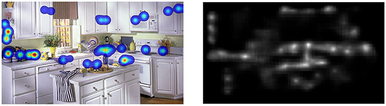
Figure 2. Example image with a heatmap for the reference, and resulting salience map. Our proposed SLCA accepts the salience map as input and is agnostic of the algorithm used to produce that map.

Methods

We tested two versions of the SLCA model—with the global and local inhibition parameter—in their ability to simulate human fixation latency in a visual search task. Both variants of the model were able to produce a sequence of fixations with predictions for both latency and location coordinates. Nonetheless, in this work we focus on the temporal aspect only since the accuracy of spatial predictions are largely influenced by the choice of model used to generate the salience map. The models were implemented in programming language Python 3 in an object-oriented style with use of additional library numpy for efficient mathematical calculations.

We also implemented a machine learning based genetic algorithm (GA) in order to find the optimal set of SLCA parameters for better model performance. The genetic algorithm belongs to a family of evolutionary algorithms and is inspired by the principles of evolution and natural selection (Mitchell, 1996). It is based on three biologically inspired computational operators: mutation, crossover and selection. Each algorithm iteration includes slightly modifying model parameters, running the model with these parameters and evaluating fitness to human data. Thus, the goal of optimization was to find the set of parameters which could help to simulate the human data more accurately. For evaluating fitness, we used Kolmogorov-Smirnov statistic as a loss function. The KS test was chosen because it has already proved its efficiency for evolutionary algorithms (see Weber et al., 2006; MacInnes, 2017).

Firstly, both variants of the SLCA model were tested with the default parameters. Then they were tested with the best parameters sets found during the GA optimization procedure. All data was divided into a training and testing set. Data of 36 participants was used for training, 10—for testing the models.

For the optimization process, 40 fixation latencies were simulated for each of 23 images for each of 36 training participants. They were gathered into a single set, as long as the human fixation latencies for each image. Then 500 values were then randomly sampled for 30 times from both human and simulation datasets. To compare their distributions, we averaged 30 KS-statistic values for these samples. The same procedure was applied for 10 test participants.

For evaluating fitness, we used Kolmogorov-Smirnov (KS) statistic chosen because it already proved its efficiency for evolutionary algorithms (see MacInnes, 2017). We used a two-sampled KS implementation from the scipy library in Python 3, which produces two values as an output: KS statistic and p-value. Thus, we attempted to minimize the KS statistic.

We ran the GA algorithm for optimization at 100 iterations (epochs). We initialized the LCA model with different parameters set, evaluated the results of each iteration with use of the KS statistic and subjected them to mutation, crossover and selection operations of GA. Throughout these iterations we attempted to optimize up to 7 parameters: (1) the leakage term λ; (2) self-excitation a; (3) input strength of the feedforward weights ρ_ij; (4) standard deviation of random noise E_i; (5) lateral inhibition $\beta \sum _{j\ne i}{x}_j$; (6) cross talk of the feedforward weights; (7) the offset f; (8) the salience multiplier term for threshold change m. To prevent overparameterization of the model, two parameters of the SLCA model were fixed: (1) the time-step size t; (2) the default activation threshold T₀.

Other fixed parameters included: (1) 40 trials, (2) maximum of 750 time steps during each trial, (3) 8,160 accumulator units with respect to the input map size.

When 100 training epochs were completed, the two variants of the SLCA model with best parameter sets found were estimated on the test set.

Results

We compared the performance of the two SLCA model variants with different implementations of the lateral inhibition parameter: (1) the original global lateral inhibition by Usher and McClelland (2001); (2) the proposed local lateral inhibition, where each unit inhibits only its immediate neighbors.

The performance of both models was evaluated with use of the two-sided Kolmogorov-Smirnov test: the data generated with a given set of parameters was compared with real human data from the visual search task. Each algorithm was run for each of 23 images and 10 test participants, which is 23 ^* 10 = 230 times in total. Both human and simulated data were gathered into two big sets. Then 500 values were randomly sampled for 30 times from both human and simulation datasets. To compare their distributions, we averaged 30 KS-statistic values for these samples. See Figure 3 for visualization of distributions for best data simulated by a local SLCA (Figure 3A) and a global SLCA (Figure 3B) models in comparison with the human samples.

FIGURE 3

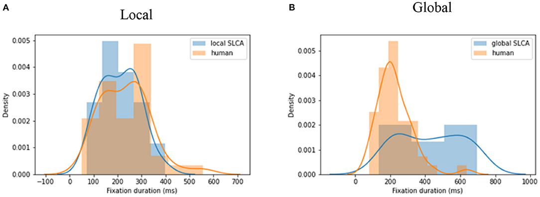
Figure 3. (A) The KS-statistic is equal to 0.08 (p <0.05) for local SLCA; (B) the KS-statistic is equal to 0.32 (p <0.05) for global SLCA.

The typical human saccadic latency distribution can be characterized by slight skewness toward longer latencies. The SLCA with local inhibition was able to simulate the basic pattern of this time-course, although it was not always able to capture the slower responses of the distribution. The final parameter set for local and global versions were tested against the human data by running 30 iterations of model results and comparing them against sampled human data. Comparisons used the KS test with alpha set to 0.05. Over 30 iterations the model simulated data that rejected the null hypothesis (human and model were different) 23 times. Thus, in 46% cases SLCA with local inhibition was able to simulate the data reliably. As for the SLCA with the original global inhibition, even with the best parameters set it was not able to reject the null hypothesis that the model and simulated data were from different distributions. The best KS value for data generated by the SLCA with local inhibition was 0.08, whereas the best KS value of the original version was 0.32. See Table 1 with the average and maximum KS statistic, for which the p <0.05.

TABLE 1

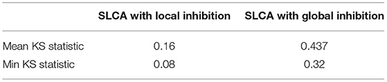
Table 1. KS statistics for SLCA with global and local inhibition.

Parameters

During the training/optimization procedure, two sets of parameters were found: for the SLCA with local and global inhibition. The optimization procedures were run for 100 epochs each. Please see Table 2 for optimal parameter sets found.

TABLE 2

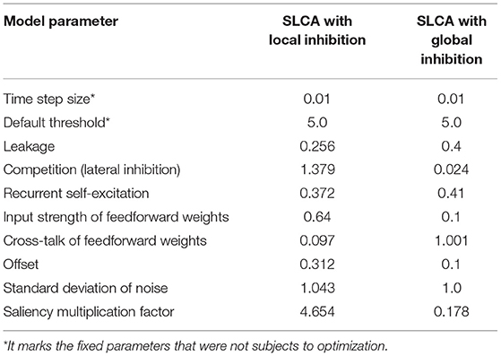
Table 2. Best parameters found via optimization.

The parameters marked with ^* were fixed. The most drastic differences can be observed in the following parameters: competition, cross-talk of feedforward weights, and saliency multiplication factor. The saliency multiplication factor defines the influence of the overall saliency of the image on the threshold. The more salient regions the image has—the greater activation threshold will be. Interestingly, the local SLCA model parameters tend to have higher thresholds.

At the same time, the value of competition, which defines the inhibition strength, was several times greater than in the global SLCA. We can suggest the following explanation to this fact: although each neuron was only inhibited by its immediate neighbors, their inhibition strength should have been comparable with the inhibition in the global SLCA model, where each neuron was inhibited by all others. Thus, the inhibitory power of each neuron should have been much greater in the SLCA model to compensate.

The model could have alternatively evolved to smaller excitation values, and we can partially observe this in cross-talk of feed-forward weights. This parameter contributes to the excitation, and it was greater in the global SLCA in comparison with the local one. It should be noted that the genetic algorithms were not guaranteed to converge to a global minimum, so the parameters could have been evolved in other ways.

Discussion

We proposed and implemented a two-dimensional version of the leaky competing accumulator (LCA) model that allowed for calculations based on neural proximity in an accumulation grid. This Spatial LCA allowed us to modify the global lateral inhibition parameter of the LCA so that only proximal neurons in the network were inhibited. We also introduced a dynamic threshold to the model, so that it could flexibly adjust to the inputs of different image average saliency. This allowed us to train and test the SLCA model on various images with various saliency with no need to adjust the parameters to each of them separately.

Finally, we tested the SLCA as a potential replacement for other spiking layers (like LIF) that are frequently used to generate shifts of attention based on a salience map generated from input images. We optimized two versions of the SLCA with global and local lateral inhibition against human fixation data from a visual foraging task.

Performance

The SLCA model with local lateral inhibition was able to generate plausible distribution of fixation latencies across the various images and participants. In contrast, the model using global lateral inhibition was not able to match human latencies on the full dataset. Lateral inhibition, as a mechanism, encourages sensitivity to variability over uniformity in the visual field. Any stimulation from a uniform visual field would equally suppress neighboring regions and thus inhibit responses. Our SLCA model with local lateral inhibition limited the interaction of spatial neurons to only those most adjacent on the two-dimensional grid. Although we use the term lateral in a literal, spatial sense, it is interesting to note that lateral inhibition is also believed to work in a more abstract sense to inhibit alternatives of non-spatial modalities (Carpenter, 1997), and this may be closer to the non-spatial implementation of the original LCA.

The model performance can be compared with other existing solutions. For instance (Merzon et al., 2020) tested the LIF algorithm used in Walther and Koch (2006) and showed that the algorithm was only able to generate latency distributions by using the inherent salience differences between the images and was unable to produce any variation in responses given a single image. This comparison holds extra validity, since Merzon and colleagues applied the LIF model to data from the same task as the current mode—reconstructing latency distribution for visual search. Although there may be room for improvement in our results, we would emphasize that by implementing neurons with spatial proximity, we were able to use lateral inhibition with limited, local scope. Although both versions of the lateral inhibition—with the local and global scope—were able to learn skewed distributions typical of human latencies, the local scope consistently was a better fit for the human data.

Lateral inhibition plays a role in saccadic responses in the intermediate layers of the superior colliculus (Munoz and Istvan, 1998), but may not need to be a component of modeling saccadic behavior. For example, Ratcliff et al. (2011) did not find evidence of inhibition in the SC, contrary to expectations. Subsequently, recent spatial models have been shown to model human temporal data without lateral inhibition (Ratcliff, 2018). Ratcliff's Spatially Continuous Diffusion Model (SCDM) uses a noise parameter added during accumulation over a spatial continuum and decisions occurring when signal reaches a planar threshold. This model was shown correctly simulate many aspects of saccadic responses including reaction time distribution and response angle to salient locations on a generated annulus. Although SCDM was not tested with salience maps generated from real images, many of the stimuli used contained salient patches amidst noise and could be comparable to the current SLCA results. Similar to our model, SCDM was not tested on sequences of saccades as this would require a suppression mechanism, like IOR, to prevent refixations on previously fixated locations. A direct comparison of results between SCDM and SLCA is not possible with the current data, but should be possible in future work and could provide a theoretical test on the utility of lateral inhibition. Another strong comparable is the recent LATEST model using Bayesian stay/go decision processes (Tatler et al., 2017). The LATEST model goes beyond simple saccadic decisions, however, and includes the creation of a full “decision map.” This map is built in LATEST using bottom up image salience in addition to top down semantic information produced by human judgements on those images. A full comparison of all recent approaches is certainly warranted, but would require a common dataset with semantic information for the LATEST model.

Spatial Predictions

Although the SLCA model generates both spatial and temporal predictions, we focused on the temporal aspect—in particular, on the latency of fixations. Our model could be used as the basis to achieve more accurate spatial predictions. First of all, if fixations are allocated according to attention on the saliency map we might implement a mechanism like inhibition of return (IOR). IOR is believed to be a foraging facilitator and a low-level mechanism that could help reduce the likelihood of revisiting previously attended locations (Klein and MacInnes, 1999; Bays and Husain, 2012; MacInnes et al., 2014; but see Smith and Henderson, 2011). This could provide insights on distributions of fixation sequences, but also improve our understanding of inhibition of return itself (Redden et al., 2021).

Bottom-Up and Top-Down Mechanisms

Our model used salience maps as the input layer to our SLCA implementations, but it was truly agnostic to the algorithm used to generate these maps. For example, we did not include any top-down attentional modulations in the current implementation, but our SLCA could easily fit as a layer on a priority map or decision map instead. Although models of bottom-up salience have produced valuable insights in visual processing, the idea of a priority map with top-down influence is closer to what we observe in human and primate biology (Fecteau and Munoz, 2006; Bisley and Goldberg, 2010). Bottom up saliency might be enough for predicting distributions of fixation latency, but locations and even order would certainly need various degrees of top down and contextual information depending on the task. When presented with real-life like scenes, the human visual system obviously makes use of top-down information, perhaps to an even greater degree than bottom up salience (Chen and Zelinsky, 2006).

Introducing top-down processes into the SLCA model could be understood as simply operating with a priority map rather than a saliency map, which means moving upwards in visual processing hierarchy and modeling feedback connections from higher structures, such as LIP or FEF. This would be similar to the approach taken by LATEST (Tatler et al., 2017) who used maps created from human judgements as a proxy for areas of semantic importance. The problem is that incorporation of top-down attention modulators would be task and scene specific and require pre-training in order to adapt a model to a particular situation, i.e., to train it for recognizing specific objects, patterns or locations. On the contrary, bottom-up saliency models do not require specific training and are able to operate with any kind of input, hence are more versatile and need no tuning for a particular task.

Behavioral and Neuronal Data

Another promising area for further research would be testing how well the SLCA could fit not only behavioral, but also neuronal data. Numerous accumulator models are based on biological principles and have been shown to match neural processing of the perceptual decision making in various brain areas, i.e., superior colliculus (Ratcliff et al., 2003, 2007). As soon as the SLCA is capable of simulating human behavioral data accurately, it could also be tested in predicting neural responses in brain areas involved in visual processing at the level of the saliency or the priority mapping, such as V1, SC, LIP, and FEF (Fecteau and Munoz, 2006; Gottlieb, 2007; Zhang et al., 2012).

Data Availability Statement

Publicly available datasets were analyzed in this study. This data can be found at: https://osf.io/9f7xe/ and https://github.com/rainsummer613/slca.

Ethics Statement

The studies involving human participants were reviewed and approved by HSE University Ethics Review Committee. The patients/participants provided their written informed consent to participate in this study.

Author Contributions

VZ and WM contributed to conception and design of the study. VZ built the model, performed the experiments, and wrote the first draft of the manuscript. WM wrote sections of the manuscript. All authors contributed to manuscript revision, read, and approved the submitted version.

Conflict of Interest

The authors declare that the research was conducted in the absence of any commercial or financial relationships that could be construed as a potential conflict of interest.

Publisher's Note

All claims expressed in this article are solely those of the authors and do not necessarily represent those of their affiliated organizations, or those of the publisher, the editors and the reviewers. Any product that may be evaluated in this article, or claim that may be made by its manufacturer, is not guaranteed or endorsed by the publisher.

Acknowledgments

This research was supported in part through computational resources of HPC facilities at HSE University (Kostenetskiy et al., 2021).

References

Abbott, L.. (1991). “Firing-rate models for neural populations,” in Neural Networks: From Biology to High-Energy Physics, eds O. Benhar, C. Bosio, P. Del Giudice, and E. Tablet (Pisa: ETS Editrice), 179–196.

Google Scholar

Adeli, H., Vitu, F., and Zelinsky, G. J. (2017). A model of the superior colliculus predicts fixation locations during scene viewing and visual search. J. Neurosci. 37, 1453–1467. doi: 10.1523/JNEUROSCI.0825-16.2016

PubMed Abstract | CrossRef Full Text | Google Scholar

Amit, D. J.. (1989). Modeling Brain Function, the World of Attractor Dynamics. Cambridge: Cambridge University Press. doi: 10.1017/CBO9780511623257

PubMed Abstract | CrossRef Full Text | Google Scholar

Bays, P. M., and Husain, M. (2012). Active inhibition and memory promote exploration and search of natural scenes. J. Vis. 12, 8. doi: 10.1167/12.8.8

PubMed Abstract | CrossRef Full Text | Google Scholar

Bisley, J. W., and Goldberg, M. E. (2010). Attention, intention, and priority in the parietal lobe. Annu. Rev. Neurosci. 33, 1–21. doi: 10.1146/annurev-neuro-060909-152823

PubMed Abstract | CrossRef Full Text | Google Scholar

Bisley, J. W., and Mirpour, K. (2019). The neural instantiation of a priority map. Curr. Opin. Psychol. 29, 108–112. doi: 10.1016/j.copsyc.2019.01.002

PubMed Abstract | CrossRef Full Text | Google Scholar

Borji, A., Sihite, D. N., and Itti, L. (2012). “Probabilistic learning of task-specific visual attention,” in 2012 IEEE Conference on Computer Vision and Pattern Recognition (Piscataway, NJ: IEEE), 470–477. doi: 10.1109/CVPR.2012.6247710

CrossRef Full Text | Google Scholar

Brown, S. D., and Heathcote, A. (2008). The simplest complete model of choice response time: Linear ballistic accumulation. Cogn. Psychol. 57, 153–178. doi: 10.1016/j.cogpsych.2007.12.002

PubMed Abstract | CrossRef Full Text | Google Scholar

Bylinskii, Z., Judd, T., Oliva, A., Torralba, A., and Durand, F. (2018). What do different evaluation metrics tell us about saliency models? IEEE Trans. Pattern Anal. Mach. Intell. 41, 740–757. doi: 10.1109/TPAMI.2018.2815601

PubMed Abstract | CrossRef Full Text | Google Scholar

Carpenter, R. H. S.. (1997). Sensorimotor processing: charting the frontier. Curr. Biol. 7, R348–R351.

PubMed Abstract | Google Scholar

Carrasco, M.. (2011). Visual attention: the past 25 years. Vis. Res. 51, 1484–1525. doi: 10.1016/j.visres.2011.04.012

PubMed Abstract | CrossRef Full Text | Google Scholar

Chelazzi, L., Miller, E. K., Duncan, J., and Desimone, R. (1993). A neural basis for visual search in inferior temporal cortex. Nature 363, 345–347. doi: 10.1038/363345a0

PubMed Abstract | CrossRef Full Text | Google Scholar

Chen, X., and Zelinsky, G. J. (2006). Real-world visual search is dominated by top-down guidance. Vis. Res. 46, 4118–4133. doi: 10.1016/j.visres.2006.08.008

PubMed Abstract | CrossRef Full Text | Google Scholar

Deng, J., Dong, W., Socher, R., Li, L. J., Li, K., and Fei-Fei, L. (2009). “Imagenet: a large-scale hierarchical image database,” in IEEE Conference on Computer Vision and Pattern Recognition (Piscataway, NJ: IEEE), 248–255. doi: 10.1109/CVPR.2009.5206848

CrossRef Full Text | Google Scholar

Fecteau, J. H., and Munoz, D. P. (2006). Salience, relevance, and firing: a priority map for target selection. Trends Cogn. Sci. 10, 382–390. doi: 10.1016/j.tics.2006.06.011

PubMed Abstract | CrossRef Full Text | Google Scholar

Gottlieb, J.. (2007). From thought to action: the parietal cortex as a bridge between perception, action, and cognition. Neuron, 53, 9–16.

PubMed Abstract | Google Scholar

Heuer, H.. (1987). Visual discrimination and response programming. Psychol. Res. 49, 91–98. doi: 10.1007/BF00308673

PubMed Abstract | CrossRef Full Text | Google Scholar

Itti, L., and Borji, A. (2013). “Computational models: bottom-up and top-down aspects,” in The Oxford Handbook of Attention, eds A. C. Nobre and S. Kastner (New York, NY: Oxford University Press), 1–20. doi: 10.1093/oxfordhb/9780199675111.013.026

CrossRef Full Text | Google Scholar

Itti, L., and Koch, C. (2000). A saliency-based search mechanism for overt and covert shifts of visual attention. Vis. Res. 40, 1489–1506. doi: 10.1016/S0042-6989(99)00163-7

PubMed Abstract | CrossRef Full Text | Google Scholar

Jagadeesh, B., Gray, C. M., and Ferster, D. (1992). Visually evoked oscillations of membrane potential in cells of cat visual cortex. Science 257, 552–554. doi: 10.1126/science.1636094

PubMed Abstract | CrossRef Full Text | Google Scholar

Jia, S., and Bruce, N. D. (2020). EML-NET: an expandable multi-layer network for saliency prediction. Image Vis. Comput. 95, 103887. doi: 10.1016/j.imavis.2020.103887

CrossRef Full Text | Google Scholar

Judd, T., Durand, F., and Torralba, A. (2012). A benchmark of computational models of saliency to predict human fixations. Available online at: http://hdl.handle.net/1721.1/68590

Google Scholar

Judd, T., Ehinger, K., Durand, F., and Torralba, A. (2009). “Learning to predict where humans look,” in 2009 IEEE 12th International Conference on Computer Vision (IEEE), 2106–2113.

Google Scholar

Kostenetskiy, P. S., Chulkevich, R. A., and Kozyrev, V. I. (2021). HPC resources of the higher school of economics. J. Phys. Conf. Ser. 1740, 012050. doi: 10.1088/1742-6596/1740/1/012050

CrossRef Full Text | Google Scholar

Krasovskaya, S., and MacInnes, W. J. (2019). Salience models: a computational cognitive neuroscience review. Vision 3, 56. doi: 10.3390/vision3040056

PubMed Abstract | CrossRef Full Text | Google Scholar

Kümmerer, M., Wallis, T. S., and Bethge, M. (2017). DeepGaze II: predicting fixations from deep features over time and tasks. J. Vis. 17, 1147. doi: 10.1167/17.10.1147

CrossRef Full Text | Google Scholar

Lennie, P.. (2003). The cost of cortical computation. Curr. Biol. 13, 493–497. doi: 10.1016/S0960-9822(03)00135-0

PubMed Abstract | CrossRef Full Text | Google Scholar

Linardos, A, Kümmerer, M., Press, O, and Bethge, M. (2021). Calibrated prediction in and out-of-domain for state-of-the-art saliency modeling. arXiv [Preprint]. arXiv:2105.12441. doi: 10.1109/ICCV48922.2021.01268

CrossRef Full Text | Google Scholar

MacInnes, W. J.. (2017). Multiple diffusion models to compare saccadic and manual responses for inhibition of return. Neural Comput. 29, 804–824. doi: 10.1162/NECO_a_00904

PubMed Abstract | CrossRef Full Text | Google Scholar

Mason, A., and Larkman, A. (1990). Correlations between morphology and electrophysiology of pyramidal neurons in slices of rat visual cortex. II. Electrophysiology. J. Neurosci. 10, 1415–1428. doi: 10.1523/JNEUROSCI.10-05-01415.1990

PubMed Abstract | CrossRef Full Text | Google Scholar

Merzon, L., Malevich, T., Zhulikov, G., Krasovskaya, S., and MacInnes, W. J. (2020). Temporal limitations of the standard leaky integrate and fire model. Brain Sci. 10, 16. doi: 10.3390/brainsci10010016

PubMed Abstract | CrossRef Full Text | Google Scholar

Mitchell, M.. (1996). An Introduction to Genetic Algorithms. Cambridge, MA: MIT Press.

Google Scholar

Munoz, D. P., and Istvan, P. J. (1998). Lateral inhibitory interactions in the intermediate layers of the monkey superior colliculus. J. Neurophysiol. 79, 1193–1209. doi: 10.1152/jn.1998.79.3.1193

PubMed Abstract | CrossRef Full Text | Google Scholar

Peters, R. J., and Itti, L. (2007). “Beyond bottom-up: incorporating task dependent influences into a computational model of spatial attention,” in 2007 IEEE Conference on Computer Vision and Pattern Recognition (Piscataway, NJ: IEEE), 1–8. doi: 10.1109/CVPR.2007.383337

CrossRef Full Text | Google Scholar

Posner, M. I.. (1980). Orienting attention. Q. J. Exp. Psychol. 32, 3–25. doi: 10.1080/00335558008248231

PubMed Abstract | CrossRef Full Text | Google Scholar

Ratcliff, R.. (2018). Decision making on spatially continuous scales. Psychol. Rev. 125, 888–935. doi: 10.1037/rev0000117

PubMed Abstract | CrossRef Full Text | Google Scholar

Ratcliff, R., Cherian, A., and Segraves, M. (2003). A comparison of macaque behavior and superior colliculus neuronal activity to predictions from models of two-choice decisions. J. Neurophysiol. 90, 1392–1407. doi: 10.1152/jn.01049.2002

PubMed Abstract | CrossRef Full Text | Google Scholar

Ratcliff, R., Hasegawa, Y. T., Hasegawa, R. P., Childers, R., Smith, P. L., and Segraves, M. A. (2011). Inhibition in superior colliculus neurons in a brightness discrimination task?. Neural Comput. 23, 1790–1820. doi: 10.1162/NECO_a_00135

PubMed Abstract | CrossRef Full Text | Google Scholar

Ratcliff, R., Hasegawa, Y. T., Hasegawa, R. P., Smith, P. L., and Segraves, M. A. (2007). Dual diffusion model for single-cell recording data from the superior colliculus in a brightness-discrimination task. J. Neurophysiol. 97, 1756–1774. doi: 10.1152/jn.00393.2006

PubMed Abstract | CrossRef Full Text | Google Scholar

Ratcliff, R., and McKoon, G. (2008). The diffusion decision model: theory and data for two-choice decision tasks. Neural Comput. 20, 873–922. doi: 10.1162/neco.2008.12-06-420

PubMed Abstract | CrossRef Full Text | Google Scholar

Redden, R. S., MacInnes, W. J., and Klein, R. M. (2021). Inhibition of return: an information processing theory of its natures and significance. Cortex 135, 30–48. doi: 10.31234/osf.io/s29f5

PubMed Abstract | CrossRef Full Text | Google Scholar

Russell, B. C., Torralba, A., Murphy, K. P., and Freeman, W. T. (2008). LabelMe: a database and web-based tool for image annotation. Int. J. Comput. Vis. 77, 157–173. doi: 10.1007/s11263-007-0090-8

CrossRef Full Text | Google Scholar

Smith, P. L.. (1995). Psychophysically principled models of visual simple reaction time. Psychol. Rev. 102, 567. doi: 10.1037/0033-295X.102.3.567

CrossRef Full Text | Google Scholar

Smith, T. J., and Henderson, J. M. (2011). Looking back at Waldo: oculomotor inhibition of return does not prevent return fixations. J. Vis. 11, 3. doi: 10.1167/11.1.3

PubMed Abstract | CrossRef Full Text | Google Scholar

Sun, Y., and Fisher, R. (2003). Object-based visual attention for computer vision. Art. Intell. 146, 77–123. doi: 10.1016/S0004-3702(02)00399-5

CrossRef Full Text | Google Scholar

Tatler, B. W., Brockmole, J. R., and Carpenter, R. H. (2017). LATEST: a model of saccadic decisions in space and time. Psychol. Rev. 124, 267. doi: 10.1037/rev0000054

PubMed Abstract | CrossRef Full Text | Google Scholar

Torralba, A., Oliva, A., Castelhano, M. S., and Henderson, J. M. (2006). Contextual guidance of eye movements and attention in real-world scenes: the role of global features in object search. Psychol. Rev. 113, 766. doi: 10.1037/0033-295X.113.4.766

PubMed Abstract | CrossRef Full Text | Google Scholar

Trappenberg, T. P., Dorris, M. C., Munoz, D. P., and Klein, R. M. (2001). A model of saccade initiation based on the competitive integration of exogenous and endogenous signals in the superior colliculus. J. Cogn. Neurosci. 13, 256–271. doi: 10.1162/089892901564306

PubMed Abstract | CrossRef Full Text | Google Scholar

Treisman, A. M., and Gelade, G. (1980). A feature-integration theory of attention. Cogn. Psychol. 12, 97–136. doi: 10.1016/0010-0285(80)90005-5

PubMed Abstract | CrossRef Full Text | Google Scholar

Usher, M., and McClelland, J. L. (2001). The time course of perceptual choice: the leaky, competing accumulator model. Psychol. Rev. 108, 550. doi: 10.1037/0033-295X.108.3.550

PubMed Abstract | CrossRef Full Text | Google Scholar

Van Essen, D. C., Lewis, J. W., Drury, H. A., Hadjikhani, N., Tootell, R. B., Bakircioglu, M., et al. (2001). Mapping visual cortex in monkeys and humans using surface-based atlases. Vision Res. 41, 1359–1378. doi: 10.1016/s0042-6989(01)00045-1

PubMed Abstract | CrossRef Full Text | Google Scholar

Walther, D., and Koch, C. (2006). Modeling attention to salient proto-objects. Neural Netw. 19, 1395–1407. doi: 10.1016/j.neunet.2006.10.001

PubMed Abstract | CrossRef Full Text | Google Scholar

Weber, M. D., Leemis, L. M., and Kincaid, R. K. (2006). Minimum Kolmogorov–Smirnov test statistic parameter estimates. J. Stat. Comput. Simul. 76, 195–206. doi: 10.1080/00949650412331321098

CrossRef Full Text | Google Scholar

Wolfe, J. M., and Gray, W. (2007). “Guided search 4.0,” in Integrated Models of Cognitive Systems, ed W. D. Gray (New York, NY: Oxford University Press), 99–119. doi: 10.1093/acprof:oso/9780195189193.003.0008

CrossRef Full Text | Google Scholar

Zhang, X., Zhaoping, L., Zhou, T., and Fang, F. (2012). Neural activities in V1 create a bottom-up saliency map. Neuron 73, 183–192. doi: 10.1016/j.neuron.2011.10.035

PubMed Abstract | CrossRef Full Text | Google Scholar

Zhao, Q., and Koch, C. (2011). Learning a saliency map using fixated locations in natural scenes. J. Vis. 11, 9. doi: 10.1167/11.3.9

PubMed Abstract | CrossRef Full Text | Google Scholar

Zhaoping, L., and May, K. A. (2007). Psychophysical tests of the hypothesis of a bottom-up saliency map in primary visual cortex. PLoS Comput. Biol. 3, e62. doi: 10.1371/journal.pcbi.0030062

PubMed Abstract | CrossRef Full Text | Google Scholar