An application programming interface implementing Bayesian approaches for evaluating effect of time-varying treatment with R and Python

1. Introduction

Scientists seek to understand what works better, when, and for whom. The methods for understanding the treatment have made great advancement since the seminal papers from Rubin (1978) and Rosenbaum and Rubin (1983) laid foundation for causal inference. Now a days, non experimental data are frequently examined to estimate causal treatment effect by emulating experimental studies. However, in non experimental setting, treatment rarely is binary (0/1) and often time-varying. Yet, most of the causal inference analytical tools made available for evaluating treatment effect were devoted to simple binary treatment setting, in an effort to resembles a parallel randomized trial. In addition, little attention has been paid to address additional challenges of missing or partially observed data, which are inherent features of real-world data.

Simple binary treatment focuses on evaluating the question of “what” by comparing two alternative treatment approaches. The generalized propensity score methods have been proposed to extend the treatment beyond binary, but not able to deal with the various time of exposure (Hirano and Imbens, 2004; Imai and Dyk, 2004). Consider time aspect of treatment, there are two types of treatment strategies: adaptive and non-adaptive. The non-adaptive treatment strategy may involve different treatment at different time over different duration, but the treatment decision is made ahead of time, not adjusted post initial assignment. A typical example of non-adaptive time-varying treatment is a multi-staged treatment protocol. For example, a surgery protocol may require patients to first go through a preoperational preparation before operation, which may be followed up by a rehabilitation program post-surgery. More often, time-varying treatment is adaptive. The adaptive treatment strategy (ATS) varies over time, and the decision for the later time point is made adaptive given the responses to the previous treatment. ATS is a common practice when treating patients with chronic condition. A second-line medication is assigned when a patient fail to respond to the first-line treatment; or the initial treatment dosage may be adjusted up or down based on how well the patient has been progressing. Because the ATS could not be predetermined ahead of time, rather the next treatment decision is made adaptive according to the new information obtained from the previous course of treatment, treatment effect evaluation of ATS requires special handling (Robins et al., 2000; Robins and Hernán, 2009).

Under the commonly adopted causal assumptions (Rosenbaum and Rubin, 1983), Bayesian causal inference attempts to uncover the “science mechanisms” underlying the potential outcomes by directly modeling the observed outcomes given treatments and individual characteristics (Rubin, 1978). Bayesian causal inference can mitigate the issue of model misspecification by taking advantage of the flexibility of Bayesian nonparametric modeling. Studies demonstrated that the Bayesian additive regression tree (BART) (Chipman et al., 2010) method performs better than some of commonly adopted propensity score methods for estimating averaged causal treatment effect when the true outcomes model is nonlinear (Hill, 2011) or when there exists heterogeneous treatment effects (Hill et al., 2020).

In addition to BART, a Bayesian Gaussian process (GP) regression model has also been successfully applied to causal inference in adaptive treatment settings (Xu et al., 2016). Huang et al. (2023) suggest that a carefully designed GP covariance prior can serve as a matching tool. The performances of GP and BART in causal inference were shown to be among the top contenders in the 2019 Atlantic Causal Inference Data Challenge (ACIC, 2019). Extensive simulation studies demonstrated that the GP and BART perform well in various settings and often show significantly better results than some commonly used causal inference methods in both non-adaptive and adaptive time-varying treatment settings (Huang, 2020; Huang et al., 2023).

Many causal inference packages are now made available. To name a few, there are twang (Cefalu et al., 2021), MatchIt (Ho et al., 2011), and causalweight (Bodory et al., 2023), available in the Comprehensive R Archive Network (CRAN). Packages available in Python include Causalinference (Wong, 2015), DoWhy (Sharma and Kiciman, 2019), Causal ML (Chen et al., 2020) and causalimpact (Brodersen et al., 2014). Most of the packages only consider binary type intervention that is assigned at one time point. To the best of our knowledge, ltmle (Lendle et al., 2017) is the only causal inference package made available for evaluating the averaged causal treatment effect for time-varying treatment strategies. The package DynTxRegime (Holloway et al., 2023) implements a learning algorithm designed to search for the best time-varying treatment strategies, rather than estimating causal treatment effect for an ATS. Both ltmle and DynTxRegime are non-Bayesian approaches. To the best of our knowledge, bartCause (Dorie and Hill, 2020) is the only Bayesian's approach which implemented BART for binary type of treatment. Many packages are also made available for handling missing data and/or partially observed data (van Buuren and Groothuis-Oudshoorn, 2011; Stekhoven and Buehlmann, 2012). However, no existing causal inference package is currently made available to handle both time-varying, missing and/or partially observed data.

The PCATS (Patient Centered Adaptive Treatment Strategy) application programming interface (API) was build to implement two Bayesian nonparametric methods, GP and BART regression, for estimating averaged causal treatment effect under general types of treatment strategies, with capacity to handle missing or partially observed data. The representational state transfer (REST) API is a standard way of interacting with applications for the purpose of processing data using a script or integrating different services or architectures. Our REST API allows users to submit data for processing and retrieve results anywhere as long as the user is connected to the internet. It can be called from different computing environments such as R, Python, or SAS as long as there is an HTTP capacity. The PCATS API is a two-tired system, with the middleware server hosts the REST API endpoints responding to API calls and the backend computational server perform and managing jobs in the queue. The API package can be called using R and Python, the two most commonly used statistical computing software.

The goal of the paper is to introduce PCATS API for estimating averaged causal treatment effects of time-varying treatment considering a two-stage setting, i.e., treatment decisions are made at two time-points, and capable of handling missing or partially observed data. Two real application examples are presented to demonstrate usage of API. The rest of the paper is organized as follows. Section 2 provides an overview of Bayesian GP and BART causal inference methods. Section 3 describes the use of PCATS to evaluate a non-adaptive treatment strategy where the exposure time may vary. Data extracted from electronic health care records are use for evaluating the effectiveness of an early aggressive treatment strategies vs. the more conventional conservative approach caring for children with JIA. In the same example, we also presented the handling of challenges for bounded summary score outcomes, a type of partially observed data, and missing data using API. Section 4 presents an example of estimating treatment effect from a pragmatic trial where treatment switching occurred at different point of the study. Section 5 discusses API design considerations, and presents simulation studies on the performance of PCATS bench-marking against ltmle under a two-stage ATS treatment setting where treatment decisions are made at a fixed time. Finally, Section 6 provide summaries and discussion as well as future directions. The Appendix section provides the functions included in the PCATS, and example codes in R and Python.

2. Methods

The Gaussian process (GP) regression fits the outcome by defining a distribution over functions in whose space the inference is directly made. It can model a highly complex dynamic system with many desirable mathematical properties. For this reason, the GP prior has been widely used to describe biological, social, financial, and physical phenomena. Unlike the linear regression, for each observation i, GP regression determines the local regression weights for each individual data point by its relative distance to the rest of the data points in the sample. The distance is determined by the GP prior covariance function, and the PCATS uses the squared exponential (SE) covariance function, which can be viewed as a general version of the Mahalanobis distance within the p-dimensional covariate spaces. It assigns a weight of near unity to the j-th individual who shares the same values of the p-dimensional covariates with the i-th individual. In other words, the GP regression would consider the j-th individual a complete match to the i-th individual in this case. The weight decreases exponentially as the distance increases, which quickly declines to 0. The rate of decline is governed by the length scale parameters of the GP prior, which is part of the model parameters to be determined by fitting the data. Therefore, the PCATS imputes the unobserved potential outcome for any given individual with a locally weighted sum of the observed outcomes from those matched (either completely or partially) individuals where the degree of matching is determined by the relative similarities of the baseline features as measured by covariates (Huang et al., 2023).

The Bayesian additive regression tree (BART) is another parameter-rich Bayesian modeling technique highly flexible to capture complex forms of the sampling distribution. It fits a sum-of-tree model to data and estimates the expected potential outcome for the i-th unit, utilizing information in adjacent data points that fall within the same leaf node of each tree. As a result, it provides a highly flexible and robust inferential tool requiring little assumption about how the outcomes are related to the covariates (Hill et al., 2020). Unlike the existing R bartCause which handles only binary type of treatment, our proposed PCATS can handle more general types of the treatment such as in the time-varying adaptive treatment strategies.

The GP regression and the BART are considered in PCATS for their proven performances in estimating averaged causal treatment effect and ability to handle general types of treatment (Hill, 2011; Huang et al., 2023). The performances of the GP regression and the BART implemented in PCATS have been extensively studied and validated for non-adaptive or adaptive treatment strategies (Huang, 2020; Huang et al., 2023). Below, we provide a brief overview of methods used to estimate the averaged treatment effect (ATE) and conditional ATE (CATE).

2.1. Non-adaptive treatment strategy

The non-adaptive treatment strategy is determined ahead of time and remains the same over the entire treatment course. Although it is static, the time of treatment exposure may not known ahead of time, and is an important determinant to the outcomes. Let $Y_i^{(a(t))}$ denote the corresponding potential outcome for the unit i resulting from exposure to the treatment a for t time duration. Let Y_i denote the observed outcome, (A_i, T_i) the observed treatment and duration of its exposure, W_i the p-dimensional prognostic variables, i.e., covariates that are determinants of the data generation mechanism of potential outcome $Y_i^{(a(t))}$, and V_i the q-dimensional baseline confounders, which are the baseline variables that are determinants to the treatment selection mechanism. The V_i and W_i may overlap. Let X_i be W_i⋃V_i, a m-dimensional baseline covariates, where m≥max(p, q). Under the stable unit treatment value assumption (SUTVA) and no unmeasured confounder assumptions, the observed outcome $Y_i=\sum _{a}I(A_i=a,T_i=t)Y_i^{(a(t))}$. Let

$\begin{array}{ll}{f}_a(x,t)=E(Y_i|A_i=a,T_i=t,X_i=x),& (1)\end{array}$

for $a\in \mathcal{A}$, and min{T_i} < = t < = max{T_i}. Under the controlled treatment condition, i..e. a = 0, f₀(x_i, t) follows either a GP or a BART prior. When taking the GP approach, the PCATS fits a Bayesian model by f_a(., t)~GP(m(w, a, t), Σ(v, t)), where the mean function m(w, a, t) is a linear equation of prognostic variables W, the assigned treatment A = a, the T exposure time, and their interaction terms. The GP covariance function is a squared exponential (SE) function of confounding variables (V, T) and ${\Sigma }_{ij}=\gamma \sum _k{(v_{k,i}-v_{k,j})}^2/l_k+{\gamma }_t{(t_i-t_j)}^2$. This structural model setup assumes that the $Y_i^{(a(t))}$ for the i-th unit is a weighted sum of the $Y_j^{(a(t))}$ for j = 1, ..., n, with the weight for each j-th unit defined by the similarity between the pair (i, j) according to their confounding variable profiles and the exposure time. When using the BART approach, the PCATS calls bartMachine in R (Kapelner and Bleich, 2016) with including all X_i as predictors in the BART model for outcome modeling. Of note, BART does not distinguish confounding variables from the prognostic variables.

In a non-experiment, units exposed to treatment a is likely to have different duration of exposure than the units exposed to the alternative treatment a′. To ensure the comparison of two treatment strategies free from the differential time, we define treatment effect at a pre-specified exposure time t_*. For each unit X_i = x, PCATS estimate causal treatment effect by contrasting the potential outcomes $\widehat{\tau }(x,t_{*})={Ŷ}_x^{(a(t_{*}))}-{Ŷ}_x^{(a^{\prime }(t_{*}))}$, where ${Ŷ}_x^{(a(t_{*}))}={\widehat{f}}_a(x,t_{*})$. The sample averaged treatment effect (ATE) is estimated by

$\begin{array}{ll}\widehat{ATE}(t_{*})=\frac{1}{n}{\displaystyle \sum _{i=1}^n}\widehat{\tau }(x_i,t_{*}).& (2)\end{array}$

The conditional ATE (CATE) is estimated for a user specified subgroup class x_k*, e.g., conditional on the age group X_k = I(Age≥65),

$\begin{array}{ll}\widehat{CATE}(t_{*})=\frac{1}{m}{\displaystyle \sum _{i\in \left\{X_{ki}=x_{k*}\right\}}}\widehat{\tau }(X_{k,i}=x_{k*},X_{-k,i}=X_{-k,i},t=t_{*}),& (3)\end{array}$

for min{T_i|x_k*} < = t_* < = max{T_i|x_k*}, where X_−k includes all the covariates other than X_k and m = #{X_ki = x_k*} is the number of the individuals meeting the subgroup classification. Of note, a can be binary, multilevel or continuous.

When making a treatment decision, we are more interested in comparing different treatment strategies with considering a minimum important margin of superiority (or inferiority). For example, when choosing between two alternative treatment strategies, patients and clinical providers wish to know if the more aggressive (presumably less safe) demonstrate sufficient benefit beyond a given superiority margin. For a user supplied meaningful margin c, the PCATS will output a new parameter describing the likelihood for one treatment demonstrates a meaningful benefit than the other above the given margin PrTE(c, t_*) = Pr(ATE(t_*) > c) in the study population. Similarly, the subgroup treatment superiority (or inferiority) can be estimated by PrCTE(c, t_*) = Pr(CATE(t_*) > c).

Table 1 outlines the algorithm in PCATS used for a non-adaptive treatment assignment. Three types of link functions are considered for the continuous outcome: identity, log, and logit functions. If log link is used, the ATE and CATE are estimated based on the log-transformed outcome, thus may be interpreted as treatment ratio. Similarly, in case of logit link, the ATE and CATE correspond to odds ratio estimates.

TABLE 1

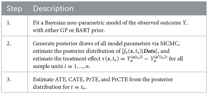
Table 1. PCATS algorithm for non-adaptive treatment assignment.

2.2. Adaptive treatment strategy

Considering a two-stage adaptive treatment strategy, let A₀ and A₁ denote treatment receive during each of the treatment stages, denoted by s = 0, 1, at the times t₁ and t₂, respectively. After treated on A₀, the next treatment A₁ is determined based on the patient responses Y₁ observed at t₁. The study endpoint outcome Y₂ is recorded at the end of t₂. For each unit i, let $Y_{1i}^{(a_0(t_1))}$ denote the potential intermediate response to the continued treatment a₀ at t₁, and $Y_{2i}^{(a_0(t_1),a_1(t_2))}$ the potential outcome given continued exposures to the treatment a₀ for t₁ duration followed by the continued treatment exposure to a₁ for t₂−t₁ duration. Let W_s denote the prognostic variables, V_s confounders, and X_s = W_s⋃V_s denote the collection of covariates at the beginning of each stage, s = 0, 1, prior to the treatment decisions were made. By following the same approach presented in Section 2.1, the PCATS estimates the posterior distribution of the missing potential outcomes at the end of each treatment stage, in a sequential generative manner, following the Bayesian's g-computation formula. At the end of the first stage, the PCATS predicts the potential intermediate outcome ${\widehat{Y}}_{1i}^{(a_0(t_{1*}))}=\widehat{E}(Y_{1i}|X_{i0},A_{i0}=a_0,T_{1i}=t_{1*})$ and the potential outcome ${\widehat{Y}}_{2i}^{(a_0(t_{1*}),a_1(t_{2*}))}=\widehat{E}(Y_{2i}|X_{i0},X_{i1},A_{i0}=a_0,A_{i1}=a_1,T_{1i}=t_{1*},T_{2i}=t_{2*})$. The potential outcomes for a given treatment history are estimated, and the ATE is estimated by the contrast between an intervention (a₀(t_1*), a₁(t_2*)) and a comparator ATS $(a_0^{\prime }(t_{1*}),a_1^{\prime }(t_{2*}))$at the final study endpoint.

The PCATS estimates the following types of averaged causal treatment effect.

• At the stage 1, the treatment effect of A₀ = a₀ vs. $A_0=a_0^{\prime }$ for a pre-specified exposure time t_1*:

$ATE(t_{1*})= E(Y_1^{(a_0(t_{1*})}-Y_1^{(a_0{}^{\text{'}}(t_{1*}))}),$

CATE(t_1*)= $E\left(Y_{1i}^{(a_0(t_{1*}))}-Y_{1i}^{(a_0^{\prime }(t_{1*}))}|X_{ki}=x_{k*}\right)$, for i ∈ {X_ki = x_k*}

PrTE(t_1*) = Pr(ATE(t_1*) > c₁), and

PrCTE(t_1*) = Pr(CATE(t_1*) > c₁)

• At the stage 2, the treatment effect of ${\text{(A}}_{\text{0}}{\text{,A}}_1{\text{) = (a}}_{\text{0}}{\text{, a}}_1\text{) vs}{\text{. (A}}_{\text{0}}{\text{,A}}_1{\text{)=(a}}_{\text{0}}{}^{\text{'}}{\text{, a}}_1{}^{\text{'}}\text{)}$ for a pre-specified exposure time t_1* and t_2* :

$\text{ATE}(t_{1*},t_{2*})= (Y_2^{(a_0(t_{1*}),a_1(t_{2*}))}-Y_2^{(a_0{}^{\text{'}}(t_{1*}),a_1{}^{\text{'}}(t_{2*}))}),$

$\begin{array}{l}\text{CATE}(t_{1*},t_{2*})=E(Y_{2i}^{(a_0(t_{1*}),a_1(t_{2*}))}-Y_{2i}^{(a_0(t_{1*}),a_1(t_{2*}))}|X_{ki}=\\ x_{k*}),\text{for }i\in \{X_{ki}=x_{k*}\}\end{array}$

PrTE(t_1*, t_2*) = Pr(ATE(t_1*, t_2*) > c₂),

PrCTE(t_1*, t_2*) = Pr(CATE(t_1*, t_2*) > c₂)

Table 2 outlines the algorithm used for a two-stage adaptive treatment assignment.

TABLE 2

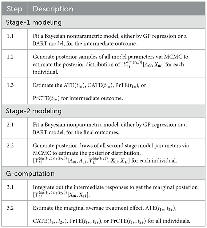
Table 2. PCATS algorithm for two-stage adaptive treatment assignment.

2.3. Handling partially observed outcome or missing data

Partially observed outcome or missing data are commonly encountered in medical and health field. The partially observed outcome can be considered as a type of measurement error where actual values falling below or above bounds were not accurately measured. Failure to appropriately account for the bounded nature of the outcome can result in a seriously biased estimate of the treatment effect. One typical example of the partially observed outcome is the bounded summary score outcome. For example, health related quality of life is defined between 0 and 100; clinician-reported or patient-reported health outcome is often on a visual analog scale of 0 and 100. Sometime, the clinical outcome measure, such as disease severity or activity score, is a summary score of several bounded measures, and thus itself is bounded. Another typical example of partially observed data is laboratory test, which is only recorded if the values fall within the upper and lower detection limits; lower or upper detection limits are recorded for values fall outside the detection limit. The time to event is a case of partially observed data as well, when the event happens before one start recording or after finish recording the event. The missing data are ubiquitous in non-experimental studies, as the data can only be recorded when the study subject interact with the recorder, or when the recorder is active. Two types of missing data problems are considered in the PCATS: missing baseline covariates and missing treatment response. This section describes the approaches implemented in the PCATS to address these issues.

2.3.1. Partially observed outcome

The PCATS conducts Bayesian GP regression directly incorporating the known bounds in the data model. Let $Y={(Y_1,...,Y_n)}^{\prime }$ denote the n-dimensional array of observed bounded outcomes for all sample units and Y^* the corresponding latent unbounded outcomes. The observed bounded outcomes and the latent unbounded outcomes are related in the following way : Y_i = LB if $Y_i^{*}\le LB$ where LB stands for the lower bound, Y_i = UB if $Y_i^{*}\ge UB$ where UB is the upper bound, and $Y_i=Y_i^{*}$ if $LB<Y_i^{*}<UB$. Let (β, Λ) denote the mean and covariance functions of the GP model, respectively. The MCMC algorithm proceeds in the following steps:

1. For i such that Y_i = LB or Y_i = UB, sample $Y_i^{*}$ from $\left[Y_i^{*}|Data,Y_{-i}^{*},\beta ,\Lambda \right]$, a normal distribution truncated below LB or above UB, i.e.,

$f\left(Y_i^{*}|Data,\beta ,\Lambda \right)=\frac{1}{{\sigma }_i}\frac{\varphi \left(\frac{Y_i^{*}-{\mu }_i}{{\sigma }_i}\right)}{\Phi \left(\frac{LB-{\mu }_i}{{\sigma }_i}\right)}\text{for}i\text{such that}{Y}_i=LB$

and

$f\left(Y_i^{*}|Data,\beta ,\Lambda \right)=\frac{1}{{\sigma }_i}\frac{\varphi \left(\frac{Y_i^{*}-{\mu }_i}{{\sigma }_i}\right)}{1-\Phi \left(\frac{UB-{\mu }_i}{{\sigma }_i}\right)}\text{for}i\text{such that}{Y}_i=UB$

where μ_i = β_i − (_{Λi, −i)1 × (n−1)} ${({\Lambda }_{-i,-i}^{-1})}_{(n-1)\times (n-1)}$ ${(Y_{-i}^{*}-{\beta }_{-i})}_{(n-1)\times 1}$ and σ_i = (_{Λi, −i)1 × (n−1)} ${({\Lambda }_{-i,-i}^{-1})}_{(n-1)\times (n-1)}$ ${({\Lambda }_{i,-i}^{\prime })}_{(n-1)\times 1}$ and the subscript −i denotes the vector/matrix except the ith element or the ith row/column. For i such that LB < Y_i < UB, set $Y_i^{*}=Y_i$.

2. Sample β, Λ from its posterior distribution [β, Λ|Data, Y^*], which is a nontruncated multivariate Guassian distribution.

3. Calculate ATE, CATE, PrTE and PrCTE as described in Table 1.

The approach assumes normal distribution of the latent outcome Y^*. When such assumption is in question, one could apply transformation to the outcome measure, and the PCATS provided a few commonly used link functions. If other transformation is more suitable given data, the user may pre-transform the data before calling the PCATS API.

For bounded summary score outcome, some commonly adopted approaches are compared in Molas and Lesaffre (2008) and Hutmacher et al. (2011). These approaches require users to first normalize the bounded summary score into 0–1 range, such that the lower bound is set at 0 and upper bound at 1. One may then apply logit or log (-log) transformation to the normalized data shifting the 0 and 1 values by a small number ϵ. The choice of ϵ value can be challenging, which may lead to different estimation results. In addition, since the treatment effect is estimated for the transformed data, its interpretation may not be straightforward. For these reasons, PCATS does not directly implement these methods. However, users may apply the methods by pre-transforming their data ahead of time before calling API.

2.3.2. Missing data

The default setting of the PCATS assumes no missing data in treatment assignment. For missing data in response variable, the PCATS first estimates the model parameters using the complete data only, and then estimates the potential outcomes for all individuals based on their baseline covariates. For the missing covariates, the PCATS allow users to supply multiple imputed baseline covariate datasets, which are pre-computed before calling API. This is because missing data computation is best performed with substantial content knowledge, and there are ample tools a user could use for generating multiple imputed (MI) data.

With the user-supplied multiple imputed datasets, the PCATS produces the estimates of ATE and CATE by combining the analysis results of each imputed dataset following the method suggested in Zhou and Reiter (2010), Si and Reiter (2011), and Gelman et al. (2013). Under the missing at random and the commonly adopted causal assumptions (Rubin, 1978; Huang et al., 2023), the ATE and CATE are summarized over all individuals in the study sample,

$\begin{array}{ll}\begin{array}{l}\widehat{ATE(t_{*})}=\frac{1}{m}{\displaystyle \sum _{l=1}^m\{\frac{1}{n}{\displaystyle \sum _{i=1}^n[{\widehat{Y}}_{li}^{(a_1(t_{*}))}-{\widehat{Y}}_{li}^{(a_0(t_{*}))}|Dat{a}_l]\},}}\hfill \end{array}& (4)\end{array}$

where l is the imputation indicator for total m multiply imputed set. Similarly, the CATE, PrTE or PrCTE can be calculated for each imputed dataset and combined.

Under the missing at random assumption, the missing response measures does not impose any particular challenges to the Bayesian's approach (Rubin, 1978). For each data units, potential outcomes are estimated using the baseline covariates., for multiply imputed covariates. The treatement effect is computed for all individuals in the study sample. The algorithm implemented in the PCATS is outlined in Table 3.

TABLE 3

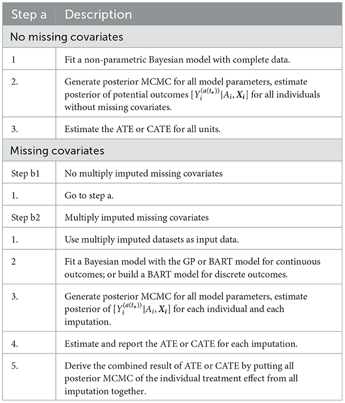
Table 3. PCATS algorithm for non-adaptive treatment assignment with missing data.

2.4. Installation of libraries in R and Python

Before calling the PCATS from R and Python, users should install the package pcatsAPIclientR in R and PCATS API python library first. The R library can be installed by the common lines below

  install.packages(‘‘pcatsAPIclientR'')

The Python library can be installed by

  python -m pip install git+https://github.com/pcats-api/pcats_api_client_py.git

 

There are three steps in calling PCATS API. The first step makes the request and retrieves the job id. The request will be sent to the API, which after initiating the execution will send back a response. The second step is to wait for the computation to finish by checking the request status using the job id. The last step fetches the results from the API. Below we demonstrate the usage of PCATS API using two case examples. Both R and Python code used in this paper can be downloaded from GitHub (https://github.com/pcats-api/pcats_api_examples/tree/main/casedata), details are provided in the Supplementary material.

3. An example of non-adaptive treatment strategy with missing covariates and bounded summary score

3.1. Research question and the study design of the JIA study

Juvenile idiopathic arthritis (JIA) is one of the most common childhood autoimmune diseases and a major cause of childhood disability. There is no cure for JIA, the management of JIA has evolved from managing pain and symptoms to targeting inactive disease, thanks to the advent of disease-modifying antirheumatic drugs (DMARDs), particularly the biologic DMARDs (bDMARD). The current clinical practice has been using conventional synthetic nonbiologic DMARDs (nbDMARDs) as the first line of treatment, followed by the bDMARD as the second line often after three months of nbDMARD. Studies suggest there might be a window of opportunity such that early and more effective treatment could lead to better outcomes faster and avoid irreversible damage to joints (Boers, 2003; Tynjälä, 2011). Randomized clinical trial offered some evidence that the early combination of biologic and nonbiologic DMARDs (n + nbDMARDs) could lead to better clinical outcomes than the nbDMARDs (Wallace et al., 2012).

Observational study can be designed to emulate randomized controlled trial to provide real-world evidence (Hernán et al., 2022). We design an observational study to emulate a randomized trial, where children newly diagnosed with JIA and were treated on nbDMARD would be randomized to the early (< 3 month) or delayed (3–6 months) initiation on bDMARD. The study utilizes data originally collected from an inception cohort study (Seid et al., 2014). Children younger than 16 years of age, newly diagnosed with JIA, being cared for at a large pediatric rheumatology clinic center were eligible to be enrolled into the study soon after being diagnosed with JIA. Patients were followed up at the 6 and 12 month after baseline, treatment and clinical variables were retrieved from patients' electronic health records and confirmed with patients by the study research coordinator. The primary outcome is JADAS10 at the 6 month follow-up. However, not all participants were followed up at the 6 months, as the follow-up visit is made conveniently for patient to be coincide with their clinical follow-up visit near the 6 month. Therefore, patients may be exposed to either one of the treatments between 119 and 462 days with median and quartile range of 173 (140, 196). Further details of the study design are reported in Seid et al. (2014). For the purpose of evaluating combination vs. nbDMARD, only a subset of patients received DMARDs prescriptions within the first 3 month were included in this CER study. The primary outcome is JADAS10 score at the 6 month of follow up.

JADAS10 is a widely used outcome measure for children with JIA (Consolaro et al., 2009). This summary disease activity score is derived from four clinical outcomes: physician's global evaluation of patient's disease activity (0–10), patient's rating of his or her wellbeing (0–10), the number of active joint counts (truncated at 10) and the standardized erythrocyte sedimentation rate or SED rate (0–10), a marker for inflammation activity. As the result, JADAS10 is bounded between 0 and 40, with lower value indicating less disease activity. The baseline covariates (see Table 4) include demographic characteristics and disease specific clinical characteristics, with 18 out of 98 patients (18.4%) missed at least one covariate measure. We imputed five sets of the missing covariates using the MICE package (van Buuren and Groothuis-Oudshoorn, 2011) and saved the imputed datasets in the example1_midata.csv file. A column named “imputation” is created in the CSV data to identify each imputed dataset.

TABLE 4

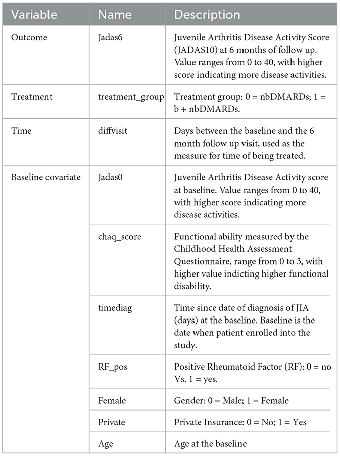
Table 4. Data description.

3.2. Calling API to estimate average treatment effect

The JIA CER study is designed to emulate a parallel arm randomized trial, thus staticGP function is used. The list of input parameters for the function are presented in Supplementary Table S2 in Appendix 2. The days of treatment exposure which was recorded in the variable diffvisit varies between 4 and 15 months. Here we describe how API can be used to estimate treatment effects at the 6 months.

We specify the outcome Jadas6 by setting outcome.type to “Continuous”, and specify outcome.bound_censor as “bounded” with the lower and upper bounds of outcome.lb=0 and outcome.ub=40. In the case of categorical outcome with two levels, users should re-code it as 0 and 1, and set outcome.type to “Discrete”. Users can define a link function by outcome.link whose default value is “identity”. The treatment identifies the treatment variable and tr.type defines the treatment type, which can take the value of “Discrete” and “Continuous”. For continuous treatment, users should input the parameters tr.values because PCATS calculates the ATE based on the user-specified values of the variable which are given by tr.values. The API will estimate treatment at the 6 month follow-up, when we specify time=diffvisit and time.value=180. The time input parameter is required, but the time.value is optional. If users do not specify time.value, then the API assigns median of diffvisit as the default value for time.value. The parameter x.explanatory specifies the prognostic variables W and x.confounding specifies the confounders V. In this example, we consider age, Female, chaq_score, RF_pos, private, Jadas0, timediag in W, and age, Jadas0, chaq_score, and timediag in V. The categorical variables in W and V should be identified in x.categorical. The mi.datafile = ~example1_midata.csv~ requests the API to calculate the ATE for each imputed dataset, and report the combined results. By default, the estimates of averaged treatment effect and potential outcomes are reported. Users can also request PrTE defined in Section 2.1 for one or a list of supplied number(s) specified by c.margin. In the example, we set c.margin to “0,1” to output PrTE(c = 0, t_* = 180) and PrTE(c = 1, t_* = 180). By default, the number of burn-in MCMC samples (burn.num) and the number of MCMC samples after burn-in (mcmc.num) are set to 500 for both. Users may specify different values for both parameters.

The output in Listing 1 presents the result of average causal treatment effect estimation. The average treatment effects (ATE) are generated based on the user-specified treatment type in tr.type. If the treatment variable is a factor, the sample potential outcomes for each level of the treatment variable are given. The pairwise comparisons of the treatment effects for all treatment groups are calculated. The first table shows the estimated ATE with standard deviation (SD), the 95% credible interval and PrTE for c.margin=(0,1) for each imputed dataset and also the summarized result. The estimate of ATE is 3.436 with the corresponding 95% equal tail credible interval (CI) of (−0.402, 7.824). The probability for b+nbDMARDs is more effective than nbDMARDs is 94.5% by a margin of 0, and 85.6% by a margine of 1. The second table presents the estimated average potential outcomes by treatment groups. The expected mean (standard deviation) for the potential outcomes are 8.043 (0.962) for nbDMARDs and 4.607 (1.574) for b+nbDMARDs, respectively. The PCATS also provides several interactive figures. Users can access these figures by using Firefox, Microsoft Edge, Chrome, or Safari. Currently, Internet Explorer does not support these figures. The histograms of MCMC posterior estimates of ATE (Figure 1) and the estimated potential outcomes (Figure 2) are presented in the URLs, which could be copied from Listing 1. The figures are interactive. By hovering the pointers, users are provided with the corresponding posterior estimates of the average treatment effect and potential outcomes. Users can hide any traces in the plot by clicking on the legend on the right side. In each histogram, users could obtain a more detailed report of the results by hovering the mouse over the specific histogram. For example, if a user is interested in finding if the probability of Y(0)−Y(1) is < 5, then (s)he could click on the pink histogram as in Figure 1, then move the mouse to the bar at ATE = 5. The user could also save the entire figure into a PNG file which can be used for sharing the results.

LISTING 1

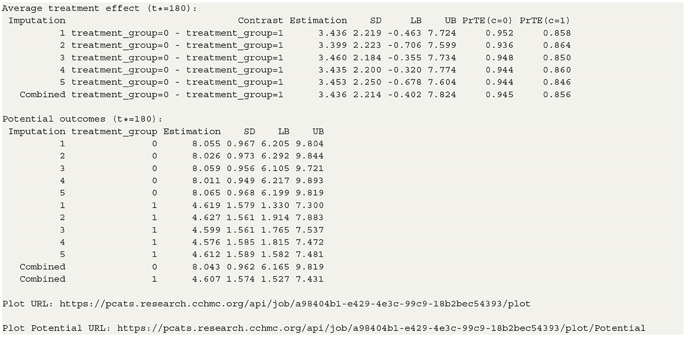
Listing 1. GP result output of example 1.

FIGURE 1

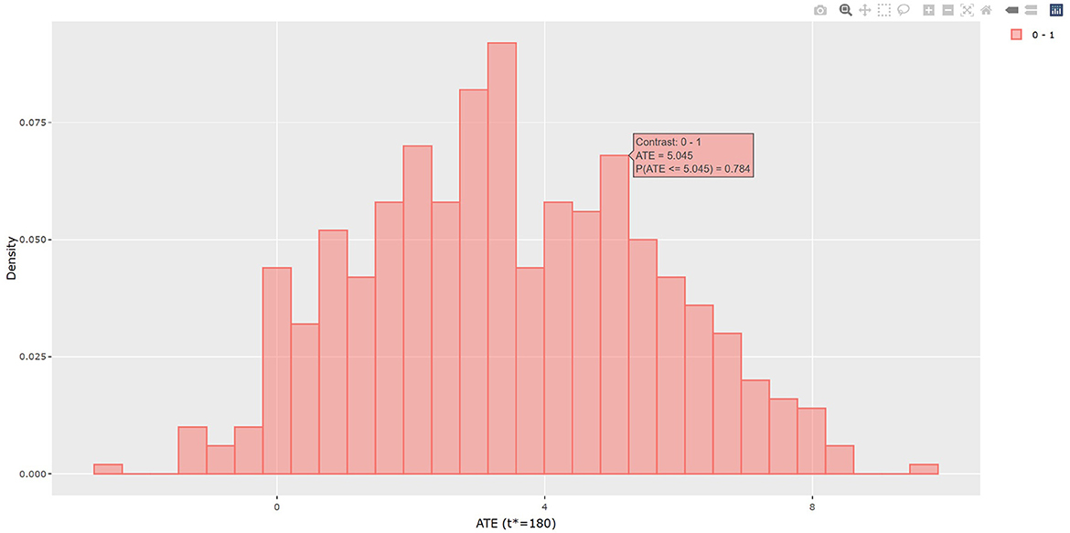
Figure 1. The histogram of the estimated average treatment effect.

FIGURE 2

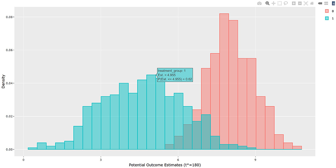
Figure 2. The histogram of the average of the estimated potential outcomes.

Users could also set method to “BART” in the staticGP function. To handle the bounded summary score of JADAS10, users may wish to first transform the JADAS10 score by mapping it onto an unbounded space following the recommendations from the current literature (e.g., Molas and Lesaffre, 2008; Hutmacher et al., 2011) before calling PCATS.

3.3. Calling API to estimate conditional average treatment effect

The PCATS can estimate the conditional average treatment effect (CATE) which captures heterogeneity of a treatment effect varying by treatment effect modifier(s). This can be accomplished by specifying the treatment effect modifier(s) for the first treatment variable with tr.hte, and for the second treatment variable with tr2.hte in the staticGP function. When specified, the corresponding interaction term(s) will be added into mean function of the GP model. In this example, by setting tr.hte =“RF_pos”, we can evaluate CATE by RF_pos.

The staticGP.cate function in R and the staticgp_cate function in Python provide the calculation of CATE (3) and PrCTE(c, t_*) for non-adaptive treatment after executing the staticGP function. The input parameters are listed in Supplementary Table S4 of Appendix 2. The conditional average treatment effects of the sample data are estimated for the user-specified treatment sub-groups. control.tr defines the reference group and treat.tr defines the treatment group compared to the reference group. Then, the estimated CATE and PrCTE and their 95% confidence intervals at each level of “RF_pos” will be reported. The R and Python codes are provided in Appendix 3.2.

The table in Listing 2 shows the estimated CATEs of the user-specified treatment groups for each level of “RF_pos”. The estimate of ATE is 2.663 (−1.669, 7.389) for the patients with negative RF and 7.716 (−1.870, 18.196) for the patients with positive RF. So the effectiveness of b+nbDMARDs compared to nbDMARDs is bigger on the patients with positive RF. The last table presents the estimated PrCTE, Pr(Y > c|Data), by “RF_pos” group. The interactive figures of the estimated CATEs in Figure 3 can be retrieved through the URL link shown at the bottom of the result in Listing 2. The violin plots show the kernel probability densities of the estimated CATEs, and the box plots show the medians of the estimated CATEs with the boxes indicating the interquartile ranges. The corresponding values are also shown in the hover text.

LISTING 2

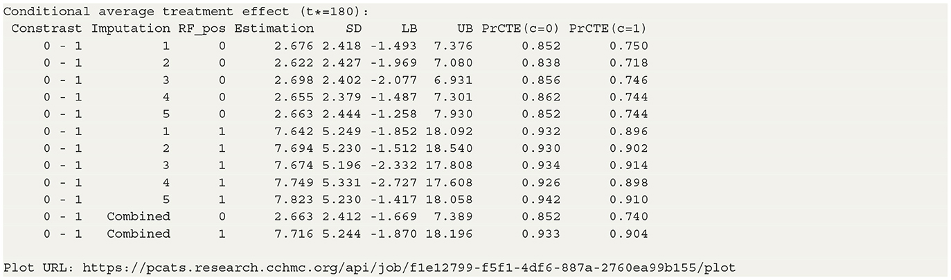
Listing 2. Result output of example 1—CATE.

FIGURE 3

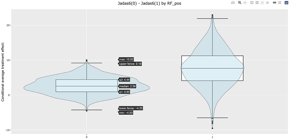
Figure 3. Estimates of the conditional average treatment effect by RF_pos.

4. An example of adaptive treatment strategy

4.1. The MOBILITY study

Weight gain is a common side effect of treatment with second-generation antipsychotics (SGA) in overweight and obese children and adolescents with bipolar spectrum disorders. Patients and parents ranked the weight gain as the top reasons for lack of adherence to SGA treatment, they are willing to start Metformin (MET) to control weight gain (Klein et al., 2020). However, the effectiveness of Metformin (MET) in mitigating weight gain remains to be established for this patient population. For this reason, the MOBILITY study (ClinicalTrials.gov, Identifier NCT02515773) is conducted. This open-label, multi-site, randomized pragmatic trial randomizes the participants in a 1:1 ratio to the intervention, i.e., MET plus healthy lifestyle intervention (MET + LIFE) or LIFE only groups. Participants are allowed to initiate or stop MET over the course of the study against the randomization. Many participants switched between treatment arms, often due to concerns over continuing weight gain. For pragmatic reasons, most of participants are followed up at their usual schedule for clinical visits, instead of following the trial protocol specified follow-up visits. As a result, the follow-up times vary greatly for participants and visits may be skipped. Examination of the data pattern suggested that many of the patients made switch at least once up to their 6 months follow-up, and their 6 month follow up ranges from 90 to 270 days. Detailed information about the study is available in Weldge et al. (2023). The data structure is shown in the Table 5.

TABLE 5

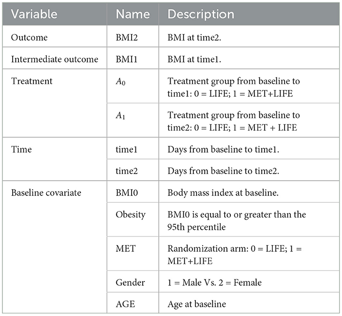
Table 5. Example 2 data description.

Because the MOBILITY trial is still ongoing, this example uses a semi-synthetic data (N = 1,200), which is designed to preserve the real-world features of this case study. Only the outcome variable is simulated based on the baseline data collected from real patients at the real follow-up time of the MOBILITY study up to the month 6 visits. First, the baseline covariates, treatment pattern, and time of follow-up were generated by a random bootstrap sampling with replacement. Second, we simulated BMI outcomes BMI1 & BMI2 at the real observed follow-up time at the point of treatment switching (time1) and up to their months 6 visit (time2). For patient who did not made treatment switch, their month 3 visit is used as the start of the stage 2. The BMI2 is set as a function of BMI1 and its interaction with the treatment. To accurately reflect the real data, we set the simulated BMI1 or BMI2 to be missing if the observed values of BMI are missing at the given visit. As a result, 43% patients missed at least one of the outcomes.

• BMI1~N(1.05*BMI0 − 0.75*A₀−0.01*time1, 1)

• $BMI2~N(-4+1.1*BMI0-A_0+0.05*BMI1+0.005*BMI{1}^2-0.5*A_1-1.5*A_0*A_1-0.08*A_1*BMI1-0.005*time2,1)$

4.2. Calling API to estimate adaptive treatment effect

The dynamicGP function is used to estimate the ATE for dynamic treatment. Since the model involves modeling of outcomes at two time-points, we require users to specify outcomes, treatment and covariates for each time. For the first time point time1, BMI1 is set to stg1.outcome and stg1.outcome.type is set to “Continuous”. The stg1.treatment identifies the treatment variable A0 and stg1.tr.type defines the type of A0, which is set to “Discrete” here. The time of exposure at time1 is specified in stg1.time, and the treatment effect is evaluated at the 3 months by setting stg1.time.value to 90 days. The parameter stg1.x.explanatory specifies the prognostic variables W and stg1.x.confounding specifies the confounders V at time1. In this example, MET, Gender, BMI0, AGE, and Obesity are put into W, and BMI0 and AGE are put into V. Similar, the input parameters at time2 can be specified. The names of these parameters all start with stg2. And stg2.time.value is set to 180 here. In addtion, stg2.tr2.hte specifies the treatment effect modifier “BMI1” for the treatment at time2, which is A1 here. The categorical variables in W and V at both time1 and time2 should be listed in x.categorical. The detailed input parameters are listed in Supplementary Table S3 of Appendix 2. The R and Python codes using BART method are shown in Appendix 3.3.

4.3. Results for MOBILITY study

The results of BART method are shown in Listing 3. The statistical results of ATE and potential outcomes at two time points are shown in the output tables. Stage 1 shows the results of the first time point and Stage 2 shows the second time point. For Stage 1, the interpretation of the result is similar to that in non-adaptive treatment. In the example, the estimated ATE and its 95% confidence interval are 0.784 (0.312, 1.162) at 90 days of treatment, which is close to the true value 0.75. At the study endpoint, the API report ATE for all six possible treatment combinations. The true values of $Y_2^{(0,0)}-Y_2^{(0,1)}$, $Y_2^{(0,0)}-Y_2^{(1,1)}$, $Y_2^{(0,0)}-Y_2^{(1,0)}$, $Y_2^{(0,1)}-Y_2^{(1,1)}$, $Y_2^{(0,1)}-Y_2^{(1,0)}$ and $Y_2^{(1,1)}-Y_2^{(1,0)}$ after 90 days of the stage 1 treatment and 90 days of the stage 2 treatment are 2.95, 5.55, 1.26, 2.61, −1.69, and −4.3. For example, the second row of Table 3 in Listing 3 provides an estimate for persistent MET treatment vs. persistent control E(Y₂(a₀(t_1* = 90) = 0, a₁(t_2* = 180) = 0))−E(Y₂(a₀(t_1* = 90) = 1, a₁(t_2* = 180) = 1)). This is the recommended per protocol effect for pragmatic trial (Hernán and Robins, 2017), which reports treatment benefit of 5.026 and the 95% credible interval is (4.447, 5.639) in BMI. All reported 95% confidence intervals cover the true values. The histogram of the estimated ATEs is shown in Figure 4. And the histogram of the estimated potential outcomes is shown in Figure 5.

LISTING 3

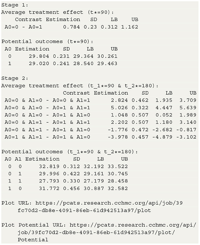
Listing 3. BART result output of example 2.

FIGURE 4

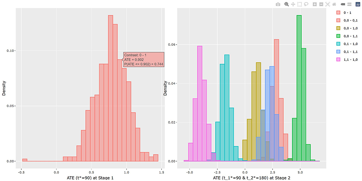
Figure 4. The histogram of the estimated average treatment effect at each stage.

FIGURE 5

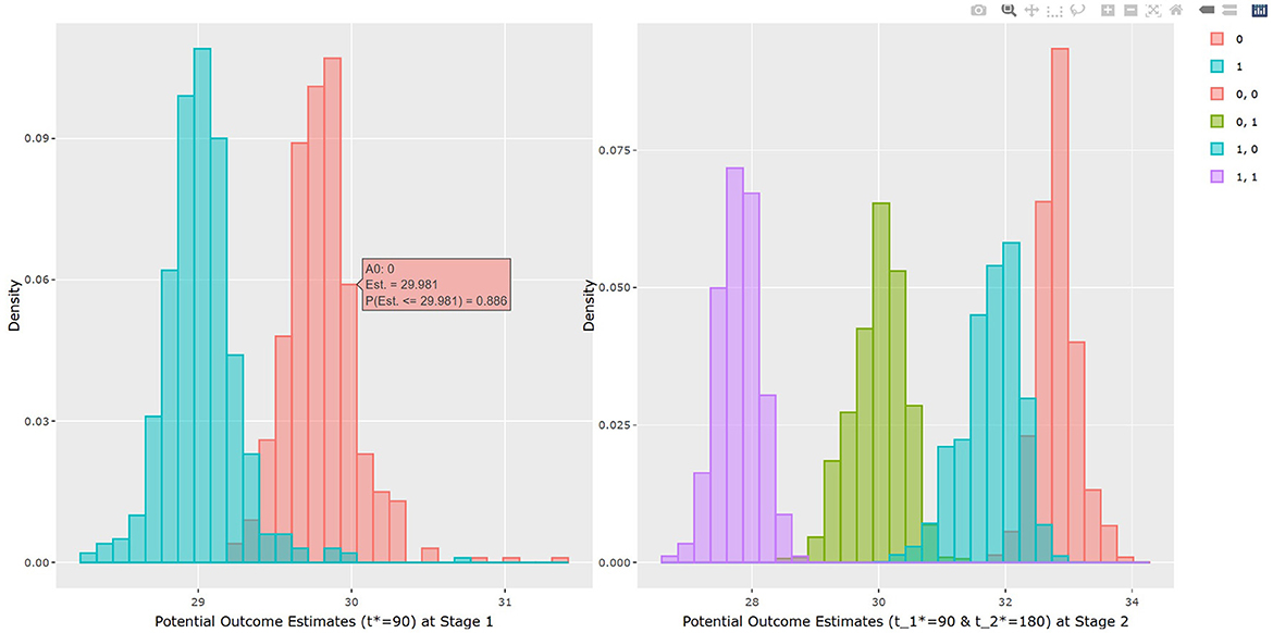
Figure 5. The histogram of the average of the estimated potential outcomes at each stage.

Similarly as in the example 1, the dynamicGP.cate function in R and the dynamicGP_cate function in Python can be used to request calculation of CATE and PrCTE for adaptive treatment. The input parameters are listed in Supplementary Table S4 of Appendix 2.

5. API architecture and benchmark performances

5.1. Design principals and architecture of API

The API is designed with the principals of clarity, consistency, robustness, extensibility and scalability in mind. The parameter names are designed to be self explanatory and consistent with the field convention. For example, we give the names of the input parameter according to the widely accepted nomenclatures in causal inference by grouping covariates into confounded and explanatory variables. Given the important role of time in the API, we made time of treatment as a distinct input parameter, rather than lump it together with the treatment variable. This also provides consistency in the sense that the treatment effect is evaluated for the treatment parameter, where as one may control the time-varying exposures by estimating treatment effect at a given fixed time t_*. On the other hand, if the research question is to comparing effect of different exposure timing, this can be accomplished by by supplying the time exposure variable name in treatment and specify tr.type = continuous. The error handling is another design principal we pay careful attentions. For example, to prevent erroneous extrapolating estimation results beyond the modeling space, any input values specified for t_* outside the observed range of T variables are considered invalid. Users will be provided corresponding suggestions. For another example, we prohibit users from inputting the same variables specified for treatment into the list of confounders. From extensibility prospective, we purposely choose to not implement missing data imputation within the API. Rather we provide functions that can compute treatment for multiply imputed data and summarize the results. This choice allows the API to keep up with the development of missing data imputation tools, while adhere to the principals of handling missing data in evaluating treatment effect. The design of API is an iterative process, version control and updated documents are important. We use GitHub repository to provided latest documentation; step-by-step users guide includes rich examples, code, and snapshot of outputs.

With scalability in mind, we design the PCATS as a two-tier system. First, the middleware server that host the REST API endpoints respond to some commands directly such as printing the results, generating plots. The second tier is the backend computational server. In general, those commands are expected to complete in a short amount of time with a very little computation are handled by the middleware server. The commands that might potentially require significant time are submitted to a queue and a handle to the submission is returned to the caller. The backend computational server handles the jobs in the queue. Users is expected to poll the status of the computations and retrieve the results when the computation is done.

This solution allows us to create an agile system with a potential to expand horizontally, i.e., add servers if the demand on the computation increases beyond the capabilities of the current single server; as well as vertically, i.e., we can add more memory or CPUs into the existing server. Similarly we can increase the redundancy and security based on the demand of the individual tasks, such as adding an authentication layer and redirecting users belonging to a particular group to a separate set of servers.

Efficiency is important. To ensure that duplicate submissions don't tie up resources unnecessarily a caching layer was introduced. We create a hash for all input parameters as well as data and if we encounter a submission with the same hash we simply return the existing results rather than going through the computation again. The storage supporting the jobs as well as the caching layer is utilizing Network File System (NFS) protocol allowing us to expand as needed as well as to maintain proper security and access controls.

5.2. Benchmark performances

One of the key feature of the PCATS is its ability to estimate causal treatment effect for time-varying adaptive treatment. To the best of our knowledge, ltmle (the longitudinal targeted maximum likelihood estimate method with ensemble machine learning) is the only existing package that is capable of handling adaptive treatment. This section presents a simple simulation study, to benchmark the performance of the GP and BART methods implemented in the PCATS, in comparison with ltmle. The simulation study uses a two-stage adaptive data generating mechanism shown below. Since ltmle does not explicitly provide causal effect estimation for a given time of follow-up, the simulation design did not include the time into the consideration. PCATS can handle this case by including time variable(s) within the dataset and set NA or a constant number (e.g., 0) for all units.

• X ~ N(0, 1)

• M ~ Bernoulli(0.4)

• A₁ ~ Bernoulli(expit(0.3 − 0.5X−0.4M))

• L₁|A₁, X, M ~ N(0.75X−0.75A₁−0.25A₁M+0.5M, 1)

• $A_2|L_1,A_1,X,M~Bernoulli(expit(0.5X+0.2A_1-0.05L_1-0.1L_1{A}_1-0.01L_1^2-0.2M))$

• $Y|A_1,X,M,L_1,A_2~N(3+0.5A_1+0.4A_{2}M-L_1-L_1^2+2A_2-A_1{A}_2+M,1)$

For GP and BART methods, the ATE effect was estimated from 2,000 posterior MCMC draws after 2,000 burn in. For the ltmle, we use the R code shown in Listing 4.

LISTING 4

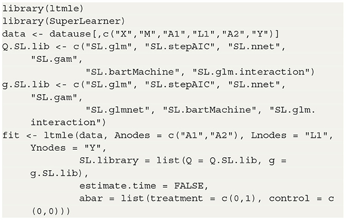
Listing 4. R code for ltmle method.

Three sample sizes were considered here, N = 200, 400, and 600. The standard deviation and the 95% confidence interval of ATE for each replicate were calculated. For comparing performances of different methods, all results were summarized over M=100 replicates by Bias $=\sum ({\widehat{\tau }}_i-\tau )/M$; median absolute error, MAE $=median\mid {\widehat{\tau }}_i-\tau \mid$; and the root mean square error, RMSE $=\sqrt{\sum {({\widehat{\tau }}_i-\tau )}^2/M}$. All six pairwise comparisons of averaged treatment effects were estimated for Y^{(0, 1)}−Y^{(0, 0)}, Y^{(1, 0)}−Y^{(0, 0)}, Y^{(1, 1)}−Y^{(0, 0)}, Y^{(1, 0)}−Y^{(0, 1)}, Y^{(1, 1)}−Y^{(0, 0)}, and Y^{(1, 1)}−Y^{(1, 0)}, and plotted against three sample sizes for each method. The results using BART, GP and LTMLE methods are presented in Figure 6, where the line plot connects the estimations for the per protocol treatment, i.e., (1, 1) vs. (0, 0). The results are also reported for each of the estimation method in Supplementary Table S5 in Appendix 4. These simulation results show that both PCATS and ltmle show similar performances in terms of bias, while the MAE and RMSE of ltmle are consistently larger than those of GP and BART.

FIGURE 6

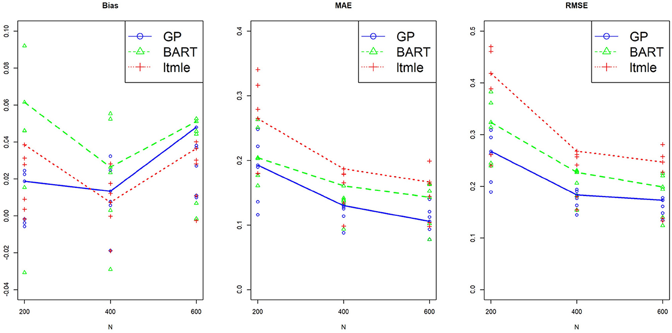
Figure 6. Performance of the suggested PCATS with GP and BART, compared with the existing R packages ltmle in two-stage adaptive data simulation settings. Bias, mean absolute error (MAE), and root mean squre error (RMSE) are compared for six all pairwise comparison averaged treatment effects over three different sample sizes N.

We further compared the computational time between the two packages. Table 6 shows the average wall time and CPU time (in seconds) of the three computation methods used in the simulation study. The BART is comparable to the LTMLE in wall and CPU times. GP's computation time, however, is significantly higher and demands more computation resources as the sample size increases.

TABLE 6

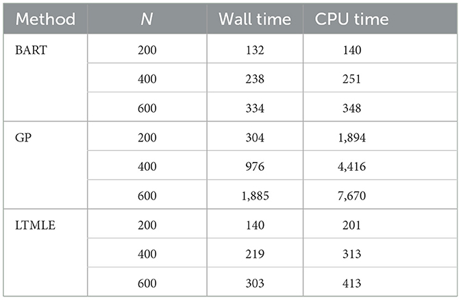
Table 6. Computation time of BART and GP in the PCATS and that of ltmle for reference in the simulation study.

This simulation study is not designed as a comprehensive study to compare general performances of two packages, but rather served as a simple example to benchmark PCATS against ltmle in the specific example. Note that ltmle requires a categorical type of treatment, does not provide estimates of CATE or more detailed information on treatment effect such as the probability of treatment benefit, and does not handle partially observed or missing data. The PCATS, on the other hand, is designed to offer detailed causal treatment effects of time-varying treatment strategies, particularly within the context of comparative effectiveness research.

6. Discussion

The PCATS is designed to implement Bayesian nonparametric causal inference methods for time-varying treatment, either adaptive or non-adaptive, involving binary, multilevel treatment, continuous treatment, and their time of exposure. Both Bayesian GP and BART are implemented, which support different features (see Table 7). We provide functionality to handle the missing responses and covariates in the PCATS, as well as partially observed outcome measures. No missing values in the treatment variables are allowed. The API is also applicable to the cases when the time exposure to treatment is fixed. With PCATS API, one can easily access the function either by calling from R or Python. More examples using R or Python are provided in the user manual at https://github.com/pcats-api/pcats_api_examples/raw/main/doc/users_manual.pdf.

TABLE 7

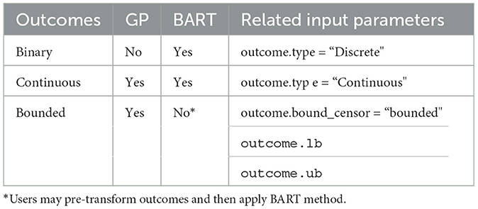
Table 7. Comparison of features for outcomes between GP and BART methods in the PCATS.

Treatment is rarely binary nor administered one-time only. More often, the treatment is taken over a period of time, and often adjusted over time. However, a few tools are available that consider the time component of a treatment when evaluating the treatment effect. PCATS includes time of exposure when estimating treatment effect, and provides the treatment effect estimated at a pre-specified exposure time. This is a major feature of the PCATS API. It provides the estimates of ATE or CATE at a user supplied time of exposure by fitting a non-parametric Bayesian model. For clinicians and patients, probability of achieving a superiority or inferiority margin is important to inform a clinical decision, and PrTE_c and PrCTE_c are provided to serve the needs. The interactive figures of treatment effects and potential outcomes are also given.

We consider the time-varying aspects of the treatment in two ways. First, for non-adaptive treatment, the treatment may vary by different time of exposure. This is illustrated in the JIA example, which utilizes data extracted from electronic health records. For adaptive treatment, the next treatment is unknown at the initial assignment, and varies by the patient's responses to the previous treatment. This is illustrated in the second example of the MOBILITY pragmatic trial. For both cases, data are not collected at the regular intervals. Instead, data is collected at the point of clinical encounters, and maybe missing due to skipped visit or missed recording. The treatment maybe switched at different time point. How to best handle time-varying dynamic treatment arise from such setting remains as a challenging topic in causal inference analyses. Our approach adheres to the currently widely accepted approaches to the design and analyses of observational study for estimating causal treatment effect. We design the JIA study targeting a parallel arm static treatment strategies as recommended in Hernán and Robins (2016) and Hernán et al. (2022). For the second example, we design and analyze the MOBILITY pragmatic trial evaluating the per protocol causal treatment effect, aiming to inform treatment effect had the treatment were adhered over the entire course (Hernán and Robins, 2017). When utilizing these real world data, it is important to ensure data quality (Huang et al., 2020). The PCATS requires the data be organized in a wide format. So there should be only one row for each individual unit. While PCATS implemented two Bayesian's approaches to estimate treatment effect following principled approach to the design and analyses of causal inference. Users should carefully evaluate the validity of fundamental causal assumptions, ensure fitness of the data, and should always exercise caution when interpreting the treatment effect estimate as causal.

A major limitation of the current version of PCATS is that it can be computationally demanding for large n or q, when GP method is used. Therefore, users are suggested to take BART for large dataset. We are working on improving the method to enhance computation efficiency. Here, we only presented a simple simulation study to compare PCATS to ltmle as the benchmark package. We refer interested readers to Hill (2011) and Huang et al. (2023) for the methodology details of using GP and BART for causal inference, and Huang (2020) for comparison of some commonly used existing methods for time-varying treatment. Future studies may consider extensive simulation studies comparing the performances of PCATS, ltmle and other compatible packages for ATS. The API is readily available for conducting additional simulation studies.

Currently, PCATS only considers a two-stage adaptive treatment assignment, focusing on estimating averaged treatment effect. However, with the posterior distribution of the model parameters, one may apply the same generative g-computation algorithm to handle the adaptive treatment with more than two stages adaptive treatment strategies. While the Bayesian method is readily extensible, scaling the API up beyond two-stage setting demands much more resources and efficient algorithms. The duration of treatment exposure is just one post-treatment time-varying confounding, more complex setting involves additional post-treatment time-varying confounders. Future development could consider addressing more complex issue. Future development could also consider introducing additional estimates, such as rank order of the best treatment options according to the estimated potential outcomes. The API development is an iterative refinement process. We intend to collaborate closely with researchers and stakeholders to further enhance the API for better providing data driven evidence that is most relevant to their decision making.

An R Shiny graphic user interface is under active development, which allows for users to upload their dataset, accessing the computational capacity of PCATS online independently from R or Python. This is beyond the current scope of the manuscript. Interested users could access GUI at https://pcats.research.cchmc.org.

Data availability statement

The datasets presented in this study can be found in online repositories. The datasets for the example 1 and the example 2 can be found at https://github.com/pcats-api/pcats_api_examples/tree/main/casedata. The simulated datasets used in the section 5.2 can be found at https://github.com/pcats-api/pcats_sim_examples/tree/main/data.

Author contributions

BH and CC: substantial contributions to the conception and design of the work and the acquisition of data. CC, BH, MK, and JL: analyses of data. CC, BH, SS, JW, and MD: interpretation of data. BH, CC, MK, HK, SS, JW, and MD: drafting the work or revising it critically for important intellectual content. CC, BH, MK, JL, HK, SS, JW, and MD: agreement to be accountable for the content of the work. All authors contributed to the article and approved the submitted version.

Funding

This work was partially supported by an award from the Patient Centered Outcome Research Institute (PCORI ME-1408-19894; PI. BH), a P&M pilot award from the Centre for Clinical and Translational Science and Training (Award Number 5UL1TR001425-03), the National Institutes of Arthritis and Musculoskeletal Skin Diseases under Award-Number P30AR076316, and an Innovation Fund award from the Cincinnati Children's Hospital Medical Center. MOBILITY was funded by the Patient Centered Outcome Research Institute (PCOR PCS 1406-19276; PI. MD).

Acknowledgments

We would like to thank clinicians and parents who care for children with JIA for motivating us to take on the patient centered adaptive treatment strategies (PCATS) project. We would like to acknowledge the MOBILITY study team, including investigators, committee members and research participants for sharing their work and data with us, for motivating us to continue development of this work.

Conflict of interest

The authors declare that the research was conducted in the absence of any commercial or financial relationships that could be construed as a potential conflict of interest.

Publisher's note

All claims expressed in this article are solely those of the authors and do not necessarily represent those of their affiliated organizations, or those of the publisher, the editors and the reviewers. Any product that may be evaluated in this article, or claim that may be made by its manufacturer, is not guaranteed or endorsed by the publisher.

Supplementary material

The Supplementary Material for this article can be found online at: https://www.frontiersin.org/articles/10.3389/fcomp.2023.1183380/full#supplementary-material

References

ACIC (2019). Annual Atlantic Causal Inference Conference - Data Challenge. Montreal, QC: ACIC.

Google Scholar

Bodory, H., Huber, M., and Kueck, J. (2023). causalweight: Estimation Methods for Causal Inference Based on Inverse Probability Weighting, R package version 1.0.4. Available online at: https://CRAN.R-project.org/package=causalweight

Google Scholar

Boers, M. (2003). Understanding the window of opportunity concept in early rheumatoid arthritis. Arthrit. Rheumatol. 48, 1771–1774. doi: 10.1002/art.11156

PubMed Abstract | CrossRef Full Text | Google Scholar

Brodersen, K. H., Gallusser, F., Koehler, J., Remy, N., and Scott, S. L. (2014). Inferring causal impact using bayesian structural time-series models. Ann. Appl. Stat. 9, 247–274. doi: 10.1214/14-AOAS788

CrossRef Full Text | Google Scholar

Cefalu, M., Ridgeway, G., McCaffrey, D., Morral, A., Griffin, B. A., and Burgette, L. (2021). twang: Toolkit for Weighting and Analysis of Nonequivalent Groups, R package version 2.5. Available online at: https://CRAN.R-project.org/package=twang

Google Scholar

Chen, H., Harinen, T., Lee, J. -Y., Yung, M., and Zhao, Z. (2020). Causalml: Python package for causal machine learning. arXiv [Preprint]. arXiv: 2002.11631.

Google Scholar

Chipman, H. A., George, E. I., and McCulloch, R. E. (2010). Bart: Bayesian additive regression trees. Ann. Appl. Stat. 4, 266–298. doi: 10.1214/09-AOAS285

PubMed Abstract | CrossRef Full Text | Google Scholar

Consolaro, A., Ruperto, N., Bazso, A., Pistorio, A., Magni-Manzoni, S., Filocamo, G., et al. (2009). Development and validation of a composite disease activity score for juvenile idiopathic arthritis. Arthri. Rheumat. 61, 658–666. doi: 10.1002/art.24516

PubMed Abstract | CrossRef Full Text | Google Scholar

Dorie, V., and Hill, J. (2020). Bartcause: Causal Inference Using Bayesian Additive Regression Trees. R Package Version 1.0–2.

Google Scholar

Gelman, A., Carlin, J. B., Stern, H. S., Dunson, D. B., Vehtari, A., and Rubin, D. B. editors. (2013). Bayesian Data Analysis. New York, NY: CRC Press.

Google Scholar

Hernán, M. A., and Robins, J. M. (2016). Using big data to emulate a target trial when a randomized trial is not available. Am. J. Epidemiol. 183, 758–764. doi: 10.1093/aje/kwv254

PubMed Abstract | CrossRef Full Text | Google Scholar

Hernán, M. A., and Robins, J. M. (2017). Per-protocol analyses of pragmatic trials. N. Engl. J. Med. 377, 1391–1398. doi: 10.1056/NEJMsm1605385

PubMed Abstract | CrossRef Full Text | Google Scholar

Hernán, M. A., Wang, W., and Leaf, D. E. (2022). Target trial emulation. JAMA 328, 2446. doi: 10.1001/jama.2022.21383

PubMed Abstract | CrossRef Full Text | Google Scholar

Hill, J., Linero, A., and Murray, J. (2020). Bayesian additive regression trees: a review and look forward. Ann. Rev. Stat. Appl. 7, 251–278. doi: 10.1146/annurev-statistics-031219-041110

CrossRef Full Text | Google Scholar

Hill, J. L. (2011). Bayesian nonparametric modeling for causal inference. J. Comput. Graph. Stat. 20, 217–240. doi: 10.1198/jcgs.2010.08162

PubMed Abstract | CrossRef Full Text | Google Scholar

Hirano, K., and Imbens, G. W. (2004). “The propensity score with continuous treatments,” in Applied Bayesian Modeling and Causal Inference From Incomplete-Data Perspectives. p. 73–84 doi: 10.1002/0470090456.ch7

PubMed Abstract | CrossRef Full Text | Google Scholar

Ho, D. E., Imai, K., King, G., and Stuart, E. A. (2011). MatchIt: Nonparametric preprocessing for parametric causal inference. J. Statist. Softw. 42, 1–28. doi: 10.18637/jss.v042.i08

CrossRef Full Text | Google Scholar

Holloway, S. T., Laber, E. B., Linn, K. A., Zhang, B., Davidian, M., and Tsiatis, A. A. (2023). DynTxRegime: Methods for Estimating Optimal Dynamic Treatment Regimes, R package version 4.12. Available online at: https://CRAN.R-project.org/package=DynTxRegime

Google Scholar

Huang, B. (2020). New Statistical Methods to Compare the Effectiveness of Adaptive Treatment Plans. Patient-Centered Outcomes Research Institute (PCORI). doi: 10.25302/11.2020.ME.140819894

CrossRef Full Text | Google Scholar

Huang, B., Chen, C., Liu, J., and Sivaganisan, S. (2023). Gpmatch: a bayesian causal inference approach using gaussian process covariance function as a matching tool. Front. Appl. Math. Stat. 9, 1122114. doi: 10.3389/fams.2023.1122114

CrossRef Full Text | Google Scholar

Huang, B., Qiu, T., Chen, C., Neace, A., Zhang, Y., Yue, X., et al. (2020). “Comparative effectiveness research using electronic health records data: ensure data quality,? in SAGE Research Methods Cases Medicine Health (London: SAGE Publications Ltd.).

Google Scholar

Hutmacher, M. M., French, J. L., Krishnaswami, S., and Menon, S. (2011). Estimating transformations for repeated measures modeling of continuous bounded outcome data. Stat. Methods Med. Res. 30, 935–949. doi: 10.1002/sim.4155

PubMed Abstract | CrossRef Full Text | Google Scholar

Imai, K., and Dyk, D. A. V. (2004). Causal inference with general treatment regimes: generalizing the propensity score. J. Am. Stat. Assoc. 99, 854–866. doi: 10.1198/016214504000001187

CrossRef Full Text | Google Scholar

Kapelner, A., and Bleich, J. (2016). bartMachine: Machine learning with bayesian additive regression trees. J. Statist. Softw. 70, 1–40. doi: 10.18637/jss.v070.i04

CrossRef Full Text | Google Scholar

Klein, C. C., Topalian, A. G., Starr, B., Welge, J., Blom, T., Starr, C., et al. (2020). The importance of second-generation antipsychotic-related weight gain and adherence barriers in youth with bipolar disorders: patient, parent, and provider perspectives. J. Child Adolesc. Psychopharmacol. 30, 376–380. doi: 10.1089/cap.2019.0184

PubMed Abstract | CrossRef Full Text | Google Scholar

Lendle, S. D., Schwab, J., Petersen, M. L., and Van der Laan, M. (2017). ltmle: an r package implementing targeted minimum loss-based estimation for longitudinal data. J. Stat. Softw. 81, 1–21. doi: 10.18637/jss.v081.i01

CrossRef Full Text | Google Scholar

Molas, M., and Lesaffre, E. (2008). A comparison of three random effects approaches to analyze repeated bounded outcome scores with an application in a stroke revalidation study. Stat. Methods Med. Res. 27, 6612–6633. doi: 10.1002/sim.3432

PubMed Abstract | CrossRef Full Text | Google Scholar

Robins, J. M., and Hernán, M. A. (2009). “Estimation of the causal effects of time-varying exposures,? in Longitudinal Data Analysis, eds G. Fitzmaurice, M. Davidian, G. Verbeke, and G. Molenberghs (New York, NY: Chapman and Hall/CRC Press), 553–599.

Google Scholar

Robins, J. M., Hernan, M. A., and Brumback, B. (2000). Marginal structural models and causal inference in epidemiology. Epidemiology 11, 550–560. doi: 10.1097/00001648-200009000-00011

PubMed Abstract | CrossRef Full Text | Google Scholar

Rosenbaum, P. R., and Rubin, D. B. (1983). The central role of the propensity score in observational studies for causal effects. Biometrika 70, 41–55. doi: 10.1093/biomet/70.1.41

CrossRef Full Text | Google Scholar

Rubin, D. B. (1978). Bayesian inference for causal effects: the role of randomization. Ann. Stat. 6, 34–58. doi: 10.1214/aos/1176344064

CrossRef Full Text | Google Scholar

Seid, M., Huang, B., Niehaus, S., Brunner, H. I., and Lovell, D. J. (2014). Determinants of health-related quality of life in children newly diagnosed with juvenile idiopathic arthritis. Arthrit. Care Res. 66, 263–269. doi: 10.1002/acr.22117

PubMed Abstract | CrossRef Full Text | Google Scholar

Sharma, A., and Kiciman, E. (2019). DoWhy: A Python package for causal inference, Python package version 0.9.1. Available online at: https://github.com/microsoft/dowhy

Google Scholar

Si, Y., and Reiter, J. P. (2011). A comparison of posterior simulation and inference by combining rules for multiple imputation. J. Stat. Theory Pract. 5, 335–347. doi: 10.1080/15598608.2011.10412032

CrossRef Full Text | Google Scholar

Stekhoven, D., and Buehlmann, P. (2012). Missforest - nonparametric missing value imputation for mixed-type data. Bioinformatics 28, 112–118. doi: 10.1093/bioinformatics/btr597

PubMed Abstract | CrossRef Full Text | Google Scholar

Tynjälä, P. (2011). Aggressive combination drug therapy in very early polyarticular juvenile idiopathic arthritis (acute-jia): a multicentre randomised open-label clinical trial. Ann. Rheum. Dis. 70, 1605–1612. doi: 10.1136/ard.2010.143347

PubMed Abstract | CrossRef Full Text | Google Scholar

van Buuren, S., and Groothuis-Oudshoorn, K. (2011). Mice: multivariate imputation by chained equations in r. J. Stat. Softw. 45, 1–67. doi: 10.18637/jss.v045.i03

CrossRef Full Text | Google Scholar

Wallace, C. A., Giannini, E. H., Spalding, S. J., Hashkes, P. J., O'Neil, K. M., Zeft, A. S., et al. (2012). Trial of early aggressive therapy in polyarticular juvenile idiopathic arthritis. Arthrit. Rheumat. 64, 2012–2021. doi: 10.1002/art.34343

PubMed Abstract | CrossRef Full Text | Google Scholar

Weldge, J. A., Correll, C. U., Sorter, M., Blom, T., Carle, A., Huang, B., et al. (2023). Metformin for overweight and obese children with bipolar spectrum disorders treated with second-generation antipsychotics (mobility): Protocol and methodological considerations for a large pragmatic randomized clinical trial. J. Am. Acad. Child Adolesc. Psychatry Open 1, 60–73. doi: 10.1016/j.jaacop.2023.03.004

CrossRef Full Text | Google Scholar

Wong, L. (2015). Causal Inference in Python: A Vignette, Python package version 0.1.3. Available online at: https://pypi.org/project/CausalInference

Google Scholar

Xu, Y., Müller, P., Wahed, A. S., and Thall, P. F. (2016). Bayesian nonparametric estimation for dynamic treatment regimes with sequential transition times. J. Am. Stat. Assoc. 111, 921–950. doi: 10.1080/01621459.2015.1086353

PubMed Abstract | CrossRef Full Text | Google Scholar

Zhou, X., and Reiter, J. P. (2010). A note on bayesian inference after multiple imputation. Am. Stat. 64, 159–163. doi: 10.1198/tast.2010.09109

CrossRef Full Text | Google Scholar