Pneumonia detection by binary classification: classical, quantum, and hybrid approaches for support vector machine (SVM)

1 Introduction

Pneumonia is a major disease which is prevalent across the globe. Caused by the bacteria and viruses in the air we breathe, the illness affects one or both of the lungs, creating difficulty in breathing. Pneumonia accounts for more than 15% of deaths in children younger than 5 years old (World Health Organization, 2022). Therefore, early and accurate diagnosis of pneumonia is crucial to prevent death and ensure better treatment.

There are many widely used tests to diagnose pneumonia, such as chest X-rays, chest MRI, and needle biopsy of the lung. Chest X-ray imaging is the most commonly used method, as it is relatively inexpensive and non-invasive. Figure 1 shows examples of healthy and pneumonic lung X-rays. However, the examination of chest X-rays is challenging and sensitive to subjective variability. Machine learning (ML) techniques have gained popularity for solving the image classification problem and have found their use in pneumonia diagnosis as well. Support vector machine (SVM) is a widely used method for classification. We have the added advantage of being able to reframe the SVM as a Quadratic Unconstrained Binary Optimization (QUBO) problem, making it especially suitable for studying annealing methods. In this study, we computationally evaluate a variety of SVM methods, in the context of X-ray imaging for pneumonia, and compare our results against LibSVM, a state-of-the art implementation of SVM. Our main contributions include:

1. Studying a QUBO formulation of an SVM using simulated annealing (SA) and quantum annealing (QA).

2. Solving a QUBO with Gurobi and comparing with annealing methods.

3. Combining multiple weak SVMs to get a strong classification model to accommodate fewer qubits on NISQ quantum annealers.

4. Studying a hybrid quantum-classical optimization heuristic technique, Graver Augmented Multi-seed Algorithm (GAMA).

Figure 1

Figure 1. The image on the left shows a normal chest X-ray, whereas the one on the right shows lungs with pneumonia opacity (Breviglieri, 2019).

2 Related work with CNNs and SVMs

Nagashree and Mahanand (2023) compared the performance of an SVM with a few other classification algorithms, such as decision tree, naïve Bayes, and K nearest neighbor. The comparison results indicate a better performance of SVMs for diagnosing pneumonia. Darici et al. (2020) and Kundu et al. (2021) developed an ensemble framework and implemented it with deep learning models to boost their individual performance.

Many researchers have explored, using different data sets, comparing between classical and quantum machine learning algorithms. Willsch et al. (2020) introduced a method to train an SVM on a D-Wave quantum annealer and studied its performance in comparison to classical SVMs for both synthetic data and real data obtained from biology experiments. Wang et al. (2022) implemented an SVM, enhanced with quantum annealing, for two fraud detection data sets. They observed a potential advantage of using an SVM with quantum annealing, over other classical approaches, for bank loan time series data. Delilbasic et al. (2021) implemented two formulations of a quantum support vector machine (QSVM) using IBM quantum computers and D-Wave quantum annealers and compared the results for remote sensing (RS) images. Bhatia and Phillipson (2021) compared classical approach, simulated annealing, hybrid solver, and fully quantum implementations for public Banknote Authentication dataset and the Iris Dataset.

Researchers have also studied convolutional neural networks (CNN) in this context. Although it is not the focus of our study, we mention the related literature. Sirish Kaushik et al. (2020) implemented four models of CNNs and reached an accuracy of 92.3%. Nakrani et al. (2020) and Youssef et al. (2020) implemented deep learning models (different types of CNNs) to classify the data. Madhubala et al. (2021) extended the classification to more than two types of pneumonia. They used CNNs for classification and later performed augmentation to obtain the final results. Ibrahim et al. (2021) considered bacterial pneumonia, non-COVID viral pneumonia, and COVID-19 pneumonia chest X-ray images. They performed multiple experiments with binary and multi-class classification and achieved a better accuracy in identifying COVID-19 (99%) than normal pneumonia (94%).

3 Background information

3.1 QUBO formulation of SVM

Recalling that SVM is a supervised machine learning model. The hyperplane produced by the SVM maximizes its distance between the two classes. Figure 2 shows the support vectors, and the hyperplane classifies data into two classes (labels +1 and −1).

Figure 2

Figure 2. Representation of hyperplane in SVM separating two classes of data.

Given training data X ∈ ℝ^N×d and training labels Y ∈ {−1, +1}^N, where N is the number of training data points, we look for a hyperplane determined by weights, w ∈ ℝ^d, and bias, b ∈ ℝ, to separate the training data into two classes. Mathematically, the SVM is expressed as (Date et al., 2021) follows:

$\begin{array}{c}{\displaystyle \underset{w,b}{min}}\frac{1}{2}||w||{}^2,\\ \text{subject to }{y}_i(w^T{x}_i+b)\ge 1,\forall i=1,2,\dots ,N.(1)\end{array}$

where, x_i is the i-th row vector in X and y_i is the i-th element in Y. The Lagrangian function of this optimization problem is as follows:

$\begin{array}{l}\mathcal{L}(w,b,\lambda )=\frac{1}{2}||w||{}^2-{\displaystyle \sum _{i=1}^N}{\lambda }_i\left[y_i(w^T{x}_i+b)-1\right],(2)\end{array}$

where λ is the vector containing all the Lagrangian multipliers, that is, $\lambda ={\left[{\lambda }_1,\dots ,{\lambda }_N\right]}^T,\mathrm{\text{with }}{\lambda }_i\ge 0,\forall i$. Each Lagrange multiplier or support vector corresponds to one image and represents the significance of that particular image in determining the hyperplane. Converting the above primal problem to its dual form yields a QUBO (Date et al., 2021)

$\begin{array}{l}{\displaystyle \underset{\lambda }{min}}\mathcal{L}(\lambda )=\frac{1}{2}{\displaystyle \sum _{i=1}^N}{\displaystyle \sum _{j=1}^N}{\lambda }_i{\lambda }_j{y}_i{y}_j(x_i^T{x}_j)-{\displaystyle \sum _{i=1}^N}{\lambda }_i,(3)\end{array}$

with the final weights determined as

$\begin{array}{l}w={\displaystyle \sum _{i=1}^N}{\lambda }_i{y}_i{x}_i,(4)\end{array}$

$\begin{array}{l}{\displaystyle \sum _{i=1}^N}{\lambda }_i{y}_i=0,(5)\end{array}$

and λ_i, λ_j ≥ 0, ∀i, j. Since the data are linearly inseparable, we use a kernel function to plot the input data to higher dimensions and use the SVM on the higher dimensional data. The kernel matrix is defined as follows

$\begin{array}{l}{K}_{ij}=\varphi (x_i)\varphi (x_j),\forall i,j,(6)\end{array}$

where ϕ(x_i) is some function of the input vector x_i. In this study, we have used the radial basis function (RBF) as it can project data efficiently. Mathematically, the RBF is defined as follows:

$\begin{array}{l}K(x_1,x_2)=exp(-\frac{||x_1-x_2||{}^2}{2{\sigma }^2}).(7)\end{array}$

The value of σ was chosen as 50 by trial. Substituting the RBF from (7) in (3) yields the QUBO as follows:

$\begin{array}{l}{\displaystyle \underset{\lambda }{min}}\mathcal{L}(\lambda )=\frac{1}{2}{\displaystyle \sum _{i=1}^N}{\displaystyle \sum _{j=1}^N}{\lambda }_i{\lambda }_j{y}_i{y}_j(K_{ij})-{\displaystyle \sum _{i=1}^N}{\lambda }_i.(8)\end{array}$

The Lagrange multipliers should also satisfy the condition in (5). Writing (8) as a matrix yields

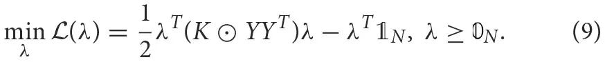
where, K is the kernel matrix whose elements are defined by (6). 𝟙_N and represent N-dimensional vectors of ones and zeros, respectively, and ⊙ is the element-wise multiplication operation. This QUBO matrix becomes the input to an annealer (Ising solver) that solves the minimization objectives and returns the Lagrange multipliers (binary) or the support vectors.

The precision vector is introduced to have integer support vectors instead of only binary, and the dimension of the precision vector depends on the range of integer values for the support vector. The precision vector has powers of 2 as elements, and here, we use p = [2⁰, 2¹] to get the final QUBO matrix. Now, the dimensions of the QUBO have doubled, and our support vectors can be four integers (0,1,2,3) instead of just being binary. Let $\widehat{\lambda }=\left[{\lambda }_{11},{\lambda }_{12},\dots ,{\lambda }_{N1},{\lambda }_{N2}\right]$ be the expanded Lagrange multiplier vector, which gives us our final QUBO. We pass the QUBO matrix to an annealer (Ising solver). The final $\widehat{\lambda }$ vector obtained minimizes the QUBO

$\begin{array}{l}{\displaystyle \underset{\widehat{\lambda }}{min}}ℒ(\widehat{\lambda })=\frac{1}{2}{\widehat{\lambda }}^T{P}^T(K\odot Y{Y}^T)P\widehat{\lambda }-{\widehat{\lambda }}^T{P}^T{\mathrm{𝟙}}_N,(10)\end{array}$

where P = I_n⊗p and $\lambda =P\widehat{\lambda }$. The annealer returns expanded Lagrange multipliers $\widehat{\lambda }$, which we use to calculate support vectors λ. We can predict the labels for unseen data using λ as follows:

$\begin{array}{l}label(x)=\text{sign}\left({\displaystyle \sum _{i=1}^N}{\lambda }_i{y}_i(K_{xi})+b\right),(11)\end{array}$

$\begin{array}{l}b=mean(y_i-w^T{x}_i),\text{ where }i\in \left[0,\dots ,N\right],\\ w^T{x}_i={\displaystyle \sum _{j=1}^N}{\lambda }_j{y}_j{K}_{ji},\end{array}(12)$

with K_xi being the kernel between the new test point x and training data point i as defined in (6).

3.2 Graver Augmented Multi-seed Algorithm (GAMA)

Let our binary optimization problem be of the form:

$\begin{array}{r}\text{objective function:}minf(x)\\ \text{constraints: }Ax=b.\end{array}$

Alghassi et al. (2019a) introduced a novel fusion of quantum and classical methodologies for computation of Graver basis. In the study by Alghassi et al. (2019b), the heuristic was given the acronym GAMA—Graver Augmented Multiseed Algorithm—and the authors studied the application of Graver basis (computed classically) as a means to attain good solutions. In this article, we explore the performance of GAMA in the context of solving an SVM.

GAMA is a heuristic algorithm, in which we compute a partial Graver basis and obtain many feasible solutions using Ising solvers. The motivation for GAMA comes from the theoretical foundation that a complete Graver basis is a Test-Set for a wide variety of objective functions (Graver, 1975; Murota et al., 2004; De Loera et al., 2009; Lee et al., 2010; Hemmecke et al., 2011). Of course, for most realistic size problems, it is not possible to identify a complete Graver basis (Pottier, 1996), but in some cases, it is much simpler to establish a partial Graver basis, especially when QUBOs are solved using Ising solvers. We therefore rely on the existence of several feasible solutions to compensate for this incompleteness of the Graver basis. Consequently, the GAMA heuristic selects the best among the (possibly) local optimal solutions by performing a (partial) Graver walk from each of the possible solutions as the seed (hence the term “multiseed”). For finding the Graver bases, we consider the QUBO form of the constraint matrix Ax = 0. The Ising solver gives us many kernel elements, and performing conformal filtration on these kernel elements gives us the partial Graver bases. To get feasible solutions, we take the QUBO form of the constraint matrix Ax = b (and solve it using an Ising solver). An alternative is to find kernel elements as differences of the feasible solutions and thus partial Graver bases and augment every feasible solution using the Graver bases to obtain solutions that are likely only a local optimum. To be clear, we have the following steps:

1. Find (partial) Graver basis (either by finding several kernel elements by solving a QUBO for Ax = 0 or taking differences of feasible solutions found in step 2);

2. Find feasible solutions by solving a QUBO for Ax = b;

3. Augment the feasible solutions using partial Graver basis elements, computing the objective function value f(x) at each step, and choosing the best solution among all (potentially) local optimal solutions.

4 Data and pre-processing

The data set used is from Kaggle (Breviglieri, 2019) (Kaggle, RRID:SCR_013852): 1,000 images from each of the normal and opacity classes are used for training the SVM, while 267 images from the normal class and 1,000 images from the opacity class are used to test the trained model for evaluation of performance. Originally, the images are of different sizes and dimensions. Therefore, the images are first resized to 200 × 200 pixels. The resized images are then flattened to give 1-dimensional arrays of 40,000 pixels.

Although the original data set in Kaggle contains more than 4,000 images, we have considered only 2,000 training images. In the dataset, we observed 1,082 normal images available for training, while there are more than 3,000 images with signs of pneumonia. To get unbiased results from the ML models, we began our training with a balanced dataset. Thus, we considered 1,000 normal images and 1,000 opacity images as the data set in our studies.

5 Methods

We begin with a discussion of each method.

5.1 Method 1: LibSVM (benchmark)

LibSVM is a state-of-the-art library that implements support vector machine (Chang and Lin, 2011) using the input data sets directly, without going through the formulation of a QUBO. The results from LibSVM are typically considered to be a benchmark to compare other newer methods.

5.2 Method 2: SVM using Gurobi

An SVM modeled as QUBO, as in (10), can be solved using a state-of-the-art classical solver, such as Gurobi (version 9.5.0). This is implemented in two ways as follows:

1. All 2,000 training images are taken at once and incorporated into the QUBO. The solver returns expanded Lagrange multipliers as an array of 4,000 elements, using which we construct 2,000 support vector values and make predictions on test data.

2. The training set is divided into 40 sets, each of 50 images. Every set represents an SVM. The 40 SVMs are solved separately and combined using majority voting bagging (Kim et al., 2002). This approach is discussed in detail in Section 5.3.

5.3 Method 3: SVM using annealing

We used the D-Wave neal simulated annealer, digital annealer from IITM, and the Advantage_system 6.2 from D-Wave with 5614 qubits with the Pegasus connectivity between them (Dattani et al., 2019) as our three Ising solver options. Among these, the first two are simulated annealers, while the latter is a quantum annealer.

With additional lenience given for the Lagrange multipliers using a precision vector, the QUBO matrix for 2,000 input images has a size of 4000 × 4000. This is beyond the processing capacity of simulated annealing using D-Wave neal and D-Wave quantum annealing. To overcome this, we opted to partition the images into 20 distinct sets, each comprising 100 images, giving a QUBO matrix of size 200 × 200, which can be solved with simulated annealers while still remaining challenging for quantum annealing platforms.

Subsequently, we refined our strategy by further dividing the images into 40 sets, each encompassing 50 images (25 from each class). As a result, there are 40 SVMs (40 QUBO matrices) of size 100 × 100. These 40 SVMs are trained separately, and their outputs are combined using the majority voting bagging technique (Kim et al., 2002) to obtain the final decision boundary for classification. This framework is presented in Figure 3.

Figure 3

Figure 3. Flowchart of the steps involved in our proposed method for utilizing SVM using annealing.

5.3.1 Method 3(a): simulated annealing

5.3.1.1 Simulated annealing using the D-Wave neal package

The 40 QUBOs corresponding to 40 SVMs are solved individually using a simulated annealer, with 1,000 iterations each per SVM. The output of the annealer is the set of expanded Lagrange multipliers for all the 1,000 iterations. We filter the one which gives the minimum energy among 1,000 iterations for every SVM and thus obtain 40 sets of expanded Lagrange multipliers for 40 SVMs, using which we get our final support vectors. The 40 SVMs are combined using the majority voting bagging technique, and the prediction of unseen test data is carried out by (11). The simulated annealer was configured using the default parameter values specified by D-Wave neal in our study.

5.3.1.2 Simulated annealing using the digital annealer of IITM

In the utilization of the Digital Annealer for simulated annealing, it was essential to designate parameter values, that is, the starting and ending temperature and iterations to perform at every temperature while descending. We converted all 40 QUBOs to Ising formulations and gave them as input to the digital annealer. The annealer performs one round of annealing from starting temperature to ending temperature with a specified number of iterations at every step. We took the initial temperature to be 6.4K, the final temperature to be 0.001K, and iterations at every step to be 20. The output we get would be the final spin values of the Ising formulation and its final energy value. We take the spin values output for all 40 SVMs which are expanded Lagrange multipliers and calculate support vectors. These are combined using majority voting, and prediction for unseen test data is done by using equation (11).

5.3.2 Method 3(b): quantum annealing

The procedure resembles that of simulated annealing with D-Wave neal. Here, instead of 1000, we have taken 500 iterations of the D-Wave quantum annealer. It is important to note that, unlike simulated annealing, quantum annealers often have substantial queue times.

5.4 Method 4: SVM using GAMA

GAMA can be a very efficient method when the objective function is complex but the constraints are simple (Alghassi et al., 2019b). We give the simpler constraints to the annealer, obtain partial Graver elements and feasible solutions, and do a walkback using the initial objective function to obtain a final solution. The constraint equation is given in (5).

To ensure that the algorithm does not get stuck in a local minimum while performing augmentation, we implement a Metropolis-Hastings version of GAMA. In this case, we consider the probability of moving in any of the directions according to the ratio in the objective function value and not just in the direction of improvement. We end the augmentation iterations if the change in objective function value remains constant for more than ten iterations.

5.4.1 Method 4(a): GAMA using simulated annealing

We tested simulated annealing from D-Wave and the Digital Annealer from IITM. Similar to the method 3 (Section 5.3), the images are divided into 40 sets (40 SVMs). Recalling that we use the constraint mentioned in (5) to get Graver bases and feasible solutions:

$\begin{array}{l}{\displaystyle \sum _{i=1}^N}{\lambda }_i{y}_i=0.(13)\end{array}$

The constraint matrix (QUBO matrix framed from the above equation) remains the same for all SVMs as the Y vector (labels vector) remains the same for all 40 SVMs (each SVM has 25 normal and then 25 opacity images). As the right-hand part of constraints is zero, kernel elements and the feasible solutions are also the same. This special structure implies that a single execution of the annealer is sufficient to address the optimization requirements for all 40 SVMs. Thus, the Graver bases and feasible solutions are obtained once and used for augmentation in all SVMs.

A total of 500 feasible solutions (also kernel elements) were obtained by simulated annealing using the D-Wave neal package (from dwave-ocean-sdk). For simulated annealing using the digital annealer of IITM, we have taken the QUBO of constraint mentioned above in (5) and converted it to an Ising formulation. The annealer performs one round of annealing at a time as mentioned in the method 3(a). We took the initial temperature to be 6.4K, the final temperature to be 0.001K, and iterations at every step to be 20. The entire annealing is performed for 500 times. Here, 500 feasible solutions (also kernel elements) are obtained. When conformal filtration is performed, we obtained 499 partial Graver bases.

Detailed experimentation of this method is performed using D-Wave neal simulated annealing. We experimented with three different sets of Graver bases and feasible solutions. The following cases are considered for augmentation:

1. 50 Graver elements + 50 feasible solutions

2. 100 Graver elements + 100 feasible solutions

3. 200 Graver elements + 200 feasible solutions

We obtained 40 sets of Lagrange multipliers corresponding to 40 SVMs for each of the three cases above. The majority of voting bagging is used to combine 40 SVMs, and the final output is tested on the test data set according to equation (11). Using the digital annealer from IITM, we have utilized all 499 partial Graver bases and feasible solutions and performed the augmentation.

5.4.2 Method 4(b): GAMA using D-Wave quantum annealing

The GAMA with quantum annealing process follows a methodology akin to that of GAMA involving simulated annealing. The number of feasible solutions was 127 (as compared with 500 in the earlier method). Notably, out of 500 calls to D-Wave, only 127 gave the minimum energy solution. All 127 feasible solutions and corresponding (partial) Graver elements (computed via conformal filtration, which happened to also be 127, likely due to the fact that the kernel elements are short to begin with) were included in the augmentation process.

6 Results and analysis

The results of various methods are compared through confusion matrix representation and associated metrics as we mentioned below. A confusion matrix is a tabular representation used to assess the performance of classification models. It provides a comprehensive overview of how well the predictions of the model align with actual outcomes for different classes or categories. The matrix is constructed by comparing predicted class labels with true class labels for data points. It represents a breakdown of the predictions into four categories: True Positives (TP) represent correctly predicted positive instances, True Negatives (TN) represent correctly predicted negative instances, False Positives (FP) represent instances that are incorrectly predicted as positive when they are actually negative, and False Negatives represent instances that are incorrectly predicted as negative when they are actually positive. The confusion matrix helps in evaluating metrics such as accuracy, precision, recall, and F1-score, which help with a deeper understanding of the performance of the model across various classes.

We evaluate various methods on four metrics as follows:

$\begin{array}{l}\text{Accuracy}=\frac{\text{TP+TN}}{\text{TP+TN+FP+FN}},(14)\end{array}$

$\begin{array}{l}\text{Precision}=\frac{\text{TP}}{\text{TP+FP}},(15)\end{array}$

$\begin{array}{l}\text{Recall}=\frac{\text{TP}}{\text{TP+FN}},(16)\end{array}$

$\begin{array}{l}\text{F1 score}=\frac{2\text{TP}}{2\text{TP+FP+FN}}.(17)\end{array}$

For all the methods, the results are noted from the confusion matrix, which is shown in Table 1 (Recalling that positive means opacity and negative is normal). For quantum annealing, the annealing time including queue time and post-processing for 40 SVMs is 3 h 16 min. In the table, we have removed all these and only provided annealing time. The metrics of comparison for all the methods are presented in Table 2.

Table 1

Table 1. Confusion matrix values and time taken for the following methods, respectively: LibSVM (Classical state-of-the-art implementation of SVM), Gurobi1 (Gurobi using all images at once), Gurobi2 (Gurobi with images split into 40 sets), SimAnn-Dn (Simulated Annealing using D-Wave neal), SimAnn-Di (Simulated Annealing using the Digital Annealer from IITM), QuantumAnn (Quantum Annealing with D-Wave), Simulated Annealing using D-Wave neal with GAMA (50 Graver + 50 feasible solutions), Simulated Annealing using D-Wave neal with GAMA (100 Graver + 100 feasible solutions), Simulated Annealing using D-Wave neal with GAMA (200 Graver + 200 feasible solutions), Simulated Annealing using the Digital annealer from IITM with GAMA (499 Graver + 499 feasible solutions), and Quantum Annealing with GAMA run on D-Wave quantum annealer (127 feasible solutions + 127 Graver elements).

Table 2

Table 2. Accuracy, precision, recall, and F1 score for all methods.

6.1 Comparison of methods

Since the running time for each method is different, we cannot draw direct comparisons based on the values of the four metrics. However, Tables 1, 2 provide insight into some key points. All the metrics from Table 2 are plotted in the graph in Figure 4 for visual convenience. We use LibSVM as the classical solver to compare our SVM implementations. As shown in Table 2, the results from other methods, especially SimAnn-Dn, compare favorably against those from LibSVM.

• Gurobi, when given data divided into 40 SVMs, takes the least time (2.44 s), but the performance is weak. When all images are input at once and trained for 30 min, there is no significant improvement in the performance.

• Simulated annealing performed using D-Wave neal takes approximately 6.5 min to run, and the results obtained are good. The best accuracy (92.5%) and F1 score (95%) are achieved with simulated annealing.

• In the case of GAMA, the performance improves as we increase the number of Graver elements taken for augmentation. The augmentation time taken also increases accordingly (it reaches a threshold value of performance as in Supplementary Figures 2, 4, See Appendix). Indeed, using 200 feasible solutions and 200 Graver elements appears sufficient to reach good performance relatively quickly.

• GAMA when implemented using quantum annealing takes approximately 8.5 min (including queue time) and provides accuracy similar to that of SVM using quantum annealing [Method 3(b)]. Here, we can observe a massive speed-up as method 3(b) takes more than 3 h to run. Thus, despite limited connectivity, GAMA provides a significant time improvement for quantum annealing, without compromising on the metrics.

• Quantum annealers often have a lower precision for encoding QUBO coefficients. However, we found that this did not affect the results because the QUBO matrix elements ranged between 0 and 2 or between 0 and 4 when we used GAMA.

Figure 4

Figure 4. Comparative analysis of accuracy, precision, recall, and F1 score for all methods.

Among our approaches, for a given time budget (of training), the best methods are as follows:

1. 5 min: GAMA 3 (200 Graver elements + 200 feasible solutions).

2. 10 min: Simulated annealing [method 3(a)] and GAMA 3 (200 Graver elements + 200 feasible solutions).

3. 20 min: Simulated annealing [method 3(a)] and GAMA 3 (200 Graver elements + 200 feasible solutions).

Not much improvement is observed by increasing training time.

6.2 Bagging and probability distribution

Majority voting bagging (Kim et al., 2002), the method used to combine SVMs, also improve the performance of the combined SVM. The accuracy of annealing methods [method 3(a) and method 3(b)] without bagging and with bagging is compared in plots (Figures 5, 6).

Figure 5

Figure 5. The yellow lines represent the accuracy metric for all the 40 SVMs we divided the data into. The red line shows the maximum accuracy achieved using weighted average bagging as 92.5%. All the SVMs are solved with simulated annealing using D-Wave neal.

Figure 6

Figure 6. The yellow lines represent the accuracy metric for all the 40 SVMs we divided the data into. The red line shows the maximum accuracy achieved using weighted average bagging as 90.3%. All the SVMs are solved using quantum annealing.

We can observe that the accuracy improved to 92.5% (Red line in Figure 5) in the case of simulated annealing using D-Wave neal and to 90.3% (Red line in Figure 6) in the case of D-Wave quantum annealing using majority voting bagging.

Many iterations of annealing are taken to find the Lagrange multipliers that best minimize the objective function value. It is instructive to know how often we might get the parameters that give the minimum objective function value. From Figures 5, 6, we also observe that some of the individual SVMs also give sufficiently good results. Thus, there maybe an opportunity to reduce computational time (by only solving a few SVMs rather than all 40) and obtain good results.

To understand the probability of obtaining the best solution, we plot the probability distribution for best-performing SVMs (for simulated annealing using D-Wave neal and quantum annealing, respectively). Figure 7 shows the probability distribution for all obtained solutions over 10,000 iterations of simulated annealing for SVM number 31, which gave us the best individual SVM accuracy. We can observe that although our desired low-energy solution occurred with low probability, the median solutions also give good accuracy. Figure 8 shows the probability distribution for all obtained solutions over 8,000 iterations of D-Wave for SVM number 27, which gave us the best individual SVM accuracy. The distribution is similar to that of simulated annealing but did not reach the quality of solutions of simulated annealing.

Figure 7

Figure 7. Probability distribution of simulated annealing solutions for SVM number 31. The best solution has energy approximately −59.

Figure 8

Figure 8. Probability distribution of D-Wave quantum annealing solutions for SVM number 27. Notably, the best solution has energy of approximately −20, not as good as that found in simulated annealing.

7 Concluding remarks

In this study, we explored binary classification through classical, quantum, and hybrid methods, using X-ray imaging data for pneumonia, and used LibSVM as our benchmark. To have a balanced data set for SVM, we selected 1,000 images, each, with and without pneumonia as our input data set. We separated the data into 40 sets. We formulated the SVM as a QUBO and solved the QUBOs using simulated annealing and Gurobi and quantum annealing. Additionally, we studied GAMA heuristic, where the (different) QUBOs were solved using simulated annealing and quantum annealing. Each of our data sets yielded an SVM. We used bagging to combine the 40 SVMs, which improved the overall accuracy.

For binary classification of X-ray images, SVM can be an alternative to CNN, especially when considering pathways to implementations on a quantum annealer. The classical solver, LibSVM, shows a 92% accuracy in classification. However, Simulated Annealing using D-Wave neal (SimAnn-Dn) has comparable or better performance. GAMA provides a speed-up over quantum annealing with the similar performance on metrics. Quantum annealing is not competitive in terms of time taken but provides solutions of quality that are near the best obtained. We anticipate an enhancement in performance when quantum annealers with more qubits and better connectivity become accessible. It is important to acknowledge that improvements in classical hardware and software are also anticipated concurrently. This suggests that periodic comparisons should be encouraged. We hope that our study adds to the literature on the benchmarking of quantum, classical, and hybrid approaches to solve a variety of important combinatorial optimization problems arising from practical applications (Metriq, 2023).

Data availability statement

Publicly available datasets were analyzed in this study. The code is found at: https://github.com/Sai-sakunthala/Pneumonia-Detection-by-Binary-Classification.

Author contributions

SG: Conceptualization, Data curation, Formal analysis, Methodology, Software, Writing – original draft. APa: Conceptualization, Data curation, Formal analysis, Methodology, Software, Writing – review & editing. APr: Funding acquisition, Supervision, Validation, Writing – review & editing. ST: Funding acquisition, Supervision, Validation, Writing – review & editing.

Funding

The author(s) declare financial support was received for the research, authorship, and/or publication of this article. The authors thank the Mphasis F1 Foundation and RAGS Foundation for supporting this study.

Conflict of interest

The authors declare that the research was conducted in the absence of any commercial or financial relationships that could be construed as a potential conflict of interest.

Publisher's note

All claims expressed in this article are solely those of the authors and do not necessarily represent those of their affiliated organizations, or those of the publisher, the editors and the reviewers. Any product that may be evaluated in this article, or claim that may be made by its manufacturer, is not guaranteed or endorsed by the publisher.

Supplementary material

The Supplementary Material for this article can be found online at: https://www.frontiersin.org/articles/10.3389/fcomp.2023.1286657/full#supplementary-material

References

Alghassi, H., Dridi, R., and Tayur, S. (2019a). Graver bases via quantum annealing with application to non-linear integer programs. arXiv [Preprint]. arxiv:1902.04215. doi: 10.48550/arXiv.1902.04215

Crossref Full Text | Google Scholar

Alghassi, H., Dridi, R., and Tayur, S. (2019b). GAMA: a novel algorithm for non-convex integer programs. arXiv [Preprint]. arxiv:1907.10930. doi: 10.48550/arXiv.1907.10930

Crossref Full Text | Google Scholar

Bhatia, H. S., and Phillipson, F. (2021). “Performance analysis of support vector machine implementations on the D-Wave quantum annealer,” in Computational Science – ICCS 2021, eds M. Paszynski, D. Kranzlmüller, V. V. Krzhizhanovskaya, J. J. Dongarra, and P. M. A. Sloot (Cham: Springer International Publishing), 84–97. doi: 10.1007/978-3-030-77980-1_7

Crossref Full Text | Google Scholar

Breviglieri, P. (2019). Pneumonia X-Ray Images. Available online at: https://www.kaggle.com/datasets/pcbreviglieri/pneumonia-xray-images (accessed August, 2023).

Google Scholar

Chang, C.-C., and Lin, C.-J. (2011). LIBSVM: a library for support vector machines. ACM Trans. Intell. Syst. Technol. 2, 27:1–27:27. doi: 10.1145/1961189.1961199

Crossref Full Text | Google Scholar

Darici, M. B., Dokur, Z., and Olmez, T. (2020). Pneumonia detection and classification using deep learning on chest X-ray images. Int. J. Intell. Syst. Appl. Eng. 8, 177–183. doi: 10.18201/ijisae.2020466310

Crossref Full Text | Google Scholar

Date, P., Arthur, D., and Pusey-Nazzaro, L. (2021). QUBO formulations for training machine learning models. Sci. Rep. 11, 10029. doi: 10.1038/s41598-021-89461-4

PubMed Abstract | Crossref Full Text | Google Scholar

Dattani, N., Szalay, S., and Chancellor, N. (2019). Pegasus: the second connectivity graph for large-scale quantum annealing hardware. arXiv [Preprint]. arxiv:1901.07636. doi: 10.48550/arXiv.1901.07636

Crossref Full Text | Google Scholar

De Loera, J., Hemmecke, R., Onn, S., Rothblum, U., and Weismantel, R. (2009). Convex integer maximization via graver bases. J. Pure Appl. Algebra 213, 1569–1577. doi: 10.1016/j.jpaa.2008.11.033

Crossref Full Text | Google Scholar

Delilbasic, A., Cavallaro, G., Willsch, M., Melgani, F., Riedel, M., and Michielsen, K. (2021). “Quantum support vector machine algorithms for remote sensing data classification,” in 2021 IEEE International Geoscience and Remote Sensing Symposium IGARSS, 2608–2611. doi: 10.1109/IGARSS47720.2021.9554802

Crossref Full Text | Google Scholar

Graver, J. E. (1975). On the foundations of linear and integer linear programming I. Math. Program. 9, 207–226.

Google Scholar

Hemmecke, R., Onn, S., and Weismantel, R. (2011). A polynomial oracle-time algorithm for convex integer minimization. Math. Program. 126, 97–117. doi: 10.1007/s10107-009-0276-7

Crossref Full Text | Google Scholar

Ibrahim, A. U., Ozsoz, M., Serte, S., Al-Turjman, F., and Yakoi, P. S. (2021). Pneumonia classification using deep learning from chest X-ray images during COVID-19. Cogn. Comput. 1–13. doi: 10.1007/s12559-020-09787-5

PubMed Abstract | Crossref Full Text | Google Scholar

Kim, H.-C., Pang, S., Je, H.-M., Kim, D., and Bang, S.-Y. (2002). “Support vector machine ensemble with bagging,” in Pattern Recognition with Support Vector Machines (Berlin; Heidelberg: Springer), 397–408. doi: 10.1007/3-540-45665-1_31

Crossref Full Text | Google Scholar

Kundu, R., Das, R., Geem, Z. W., Han, G.-T., and Sarkar, R. (2021). Pneumonia detection in chest X-ray images using an ensemble of deep learning models. PLoS ONE 16, e0256630. doi: 10.1371/journal.pone.0256630

PubMed Abstract | Crossref Full Text | Google Scholar

Lee, J., Onn, S., Romanchuk, L., and Weismantel, R. (2010). The quadratic graver cone, quadratic integer minimization, and extensions. Math. Program. 136, 301–323. doi: 10.1007/s10107-012-0605-0

Crossref Full Text | Google Scholar

Madhubala, B., Sarathambekai, S., Vairam, T., Sathya Seelan, K., Sri Sathya, R., and Swathy, A. R. (2021). “Pre-trained convolutional neural network model based pneumonia classification from chest X-ray images,” in Proceedings of the International Conference on Smart Data Intelligence (ICSMDI 2021). doi: 10.2139/ssrn.3852043

Crossref Full Text | Google Scholar

Metriq (2023). Community-Driven Quantum Benchmarks. Available online at: http://metriq.info (accessed August, 2023).

Google Scholar

Murota, K., Saito, H., and Weismantel, R. (2004). Optimality criterion for a class of nonlinear integer programs. Oper. Res. Lett. 32, 468–472. doi: 10.1016/j.orl.2003.11.007

Crossref Full Text | Google Scholar

Nagashree, S., and Mahanand, B. S. (2023). “Pneumonia chest X-ray classification using support vector machine,” in Proceedings of International Conference on Data Science and Applications, eds M. Saraswat, C. Chowdhury, C. Kumar Mandal, and A. H. Gandomi (Singapore: Springer Nature), 417–425. doi: 10.1007/978-981-19-6634-7_29

Crossref Full Text | Google Scholar

Nakrani, N. P., Malnika, J., Bajaj, S., Prajapati, H., and Jariwala, V. (2020). “Pneumonia identification using chest X-ray images with deep learning,” in ICT Systems and Sustainability, eds M. Tuba, S. Akashe, and A. Joshi (Singapore: Springer Singapore), 105–112. doi: 10.1007/978-981-15-0936-0_9

Crossref Full Text | Google Scholar

Pottier, L. (1996). “The Euclidean algorithm in dimension n,” in Proceedings of the 1996 International Symposium on Symbolic and Algebraic Computation, ISSAC '96 (New York, NY: Association for Computing Machinery), 40–42. doi: 10.1145/236869.236894

Crossref Full Text | Google Scholar

Sirish Kaushik, V., Nayyar, A., Kataria, G., and Jain, R. (2020). “Pneumonia detection using convolutional neural networks (CNNs),” in Proceedings of First International Conference on Computing, Communications, and Cyber-Security (IC4S 2019), eds P. K. Singh, W. Pawłowski, S. Tanwar, N. Kumar, J. J. P. C. Rodrigues, and M. S. Obaidat (Singapore: Springer Singapore), 471–483. doi: 10.1007/978-981-15-3369-3_36

Crossref Full Text | Google Scholar

Wang, H., Wang, W., Liu, Y., and Alidaee, B. (2022). Integrating machine learning algorithms with quantum annealing solvers for online fraud detection. IEEE Access 10, 75908–75917. doi: 10.1109/ACCESS.2022.3190897

Crossref Full Text | Google Scholar

Willsch, D., Willsch, M., De Raedt, H., and Michielsen, K. (2020). Support vector machines on the D-Wave quantum annealer. Comput. Phys. Commun. 248, 107006. doi: 10.1016/j.cpc.2019.107006

Crossref Full Text | Google Scholar

World Health Organization (2022). Pneumonia in Children. Available online at: https://www.who.int/news-room/fact-sheets/detail/pneumonia (accessed November, 2022).

Google Scholar

Youssef, T. A., Aissam, B., Khalid, D., Imane, B., and Miloud, J. E. (2020). “Classification of chest pneumonia from X-ray images using new architecture based on ResNet,” in 2020 IEEE 2nd International Conference on Electronics, Control, Optimization and Computer Science (ICECOCS), 1–5. doi: 10.1109/ICECOCS50124.2020.9314567

Crossref Full Text | Google Scholar