Is language change chiefly a social diffusion affair? The role of entrenchment in frequency increase and in the emergence of complex structural patterns

1 Introduction

Language is a system of arbitrary symbolic conventions, shared by a community of speakers. As such, language change needs to unfold through a social propagation process, akin to opinion dynamics and the diffusion of trends (Coulmont et al., 2016; Stadler et al., 2016; Michaud, 2020). In this vein, the S-curve, which is a known pattern for the diffusion of innovations, has been established as a template of language change (Weinreich et al., 1968; Johnson, 1976; Kroch, 1989; Bailey et al., 1993; Blythe and Croft, 2012). This pattern may indeed be found over a large range of disparate variables related to language change: proportion of speakers affected by a change over time (Maybaum, 2013), proportion of words affected by a phonetical change over time (Wang and Cheng, 1977), proportion of utterances showing the new variant with respect to different speakers, sorted by their propensity to use it (Bickerton, 1975), or by their age, leading to an S-curve in a so-called “apparent time” (Chambers, 1990; Gardner et al., 2020), proportion of uses of the new variant vs. the old one over time (Nevalainen, 2015), especially in the context of syntactic change (Kroch, 1989), or more simply the raw frequency of use of a given linguistic form (Krug, 2000; Mair, 2004; Fagard and Combettes, 2013). This short overview hints at the idea that ”language change” conflates a wide variety of phenomena, from purely sociolinguistic ones to phenomena that pertain to strictly structural considerations, such as changes in the phonetic system, constrained by the necessity to ensure distinctiveness between the phonemes of a given language.

The complex systems approach on language change mostly focused on the sociolinguistic side, with no small success (Loreto et al., 2011). Among other achievements, this approach showed how conventions and categories can emerge out of multiple interactions among agents (Steels, 1995; Baronchelli et al., 2010), how language can change through iterative learning as speakers get renewed over different generations (Kirby and Hurford, 2002), how a change can propagate over a speakers’ community (Dall’Asta et al., 2006; Muehlenbernd and Quinley, 2017), how new conventions that supersede prior ones may come to be adopted (Rogers, 1962; Amato et al., 2018). Nevertheless, these approaches share a common issue, coined the Threshold Problem (Nettle, 1999): for a new variant to start propagating in a speakers’ population, it requires either a) to be adopted by a fraction of speakers in the first place (Blythe and Croft, 2012; Stadler et al., 2016); or b) that some language users are specifically committed to it (Amato et al., 2018); or c) an embedded social structure of hierarchical influence (Rogers, 1962; Nettle, 1999; Blythe and Croft, 2012); or d) an external influence promoting that variant (Michard and Bouchaud, 2005; Ghanbarnejad et al., 2014; Amato et al., 2018), e.g., an institutional recommendation or a situation of language contact. Since not all new language variants are externally promoted, there needs to be some mechanisms to explain how several language users, possibly unrelated, may come up with the same new variant. In other words, there is a likelihood that new variants are intrinsically motivated within the language organization. This would explain, as well, why changes are not entirely arbitrary, and exhibit strong typological regularities (Heine, 1997; Heine and Kuteva, 2002), or why languages sharing a common ancestry tend to develop similar changes at different times (Van Peteghem, 2012).

Moreover, several aspects of language are concomitantly relevant in change. These are well articulated in the Utterance Selection Model (Baxter et al., 2006), which relies on both a social network between language users and an exemplar-based model of language for each user. Typically, language is represented as a semantic domain populated with two competing populations of tokens, tying to two different language variants that express this meaning. The frequency of use of a new variant may increase both because it spreads from one user to the next (that is, through social diffusion), and also because the speakers’ exemplar-based representations of the meaning may become increasingly filled with tokens of the new variant (that is, through an entrenchment of that variant over the semantic domain). This representation may be refined further by considering the network-like organization of language itself (Solé et al., 2010), so that a variant may spread from one semantic domain to the next, undergoing henceforth a process of lexical diffusion.

In this light, this article aims to support the following claim: the patterns of change associated with variations in token frequency as measured in historical corpora only weakly reflect social diffusion but are associated with linguistic phenomena pertaining to the complex organization of language. The goal is not to downsize the importance of sociolinguistic phenomena or to challenge the substantial results already obtained in that direction, but to emphasize that there is more to it in language change, and that frequency dynamics may help us probe the complex structure of the language system.

To substantiate this claim, this article proceeds in three steps. First, we acknowledge that historical change is usually tracked through corpora by means of token frequency, that is, by counting how often a given linguistic form shows up in texts or oral recordings. This data, however, conflates a multiplicity of factors: register specificity, lexical diffusion, social diffusion, cognitive entrenchment, etc. As such, it is unclear what we observe when we monitor language change unfolding through token frequency variations. To clarify this situation, we offer a simple formalism to make explicit three different contributions to frequency increase: an increase in prevalence (social diffusion), an increase in contexts of use (lexical diffusion), and an overall entrenchment in use, typically ranging from extravagant patterns such as snowclones (Hartmann and Ungerer, 2021) that have very low entrenchment, to grammaticalized patterns that have become fully obligatory (Bisang, 2015), and therefore maximally entrenched.

These three components map to three non-mutually exclusive hypotheses that may explain a given linguistic change. The first hypothesis is that the domain of diffusion is social: over time, more people adopt the form. The chief cause of change would then be rooted in sociolinguistic factors, situations of linguistic contact, external influences (e.g., language academies), etc. The second hypothesis is that the range of linguistic contexts in which the form is used extends over time. If the linguistic form is a variable syntactic pattern (what Construction Grammar refers to as a ’schematic construction’, such as be done + V-ing, where the V-ing can be filled with a variety of verbs), one way to describe this domain of use is to inventory the fillers that combine with the free slot of that pattern. In this case, we can refer to this domain diffusion as a lexical diffusion: over time, successive lexical items that are compatible with the open slot in the construction come to fill it. The chief drive of linguistic change in that case would be analogy. The third hypothesis is that the domain of diffusion is structural: over time, a structure that licenses all the forms of the construction together becomes progressively favored. Competition scenarios between two forms are typical instances of such a diffusion. The main cause of the change is in the emergence of a new form-function pairing that sanctions the uses of the linguistic form over a particular domain of use that corresponds to the new function.

The second step of our paper aims to disentangle these three hypotheses, based on empirical data from the French textual database Frantext (ATILF, 1998) for 25 different schematic constructions undergoing a clear change episode in their historical course. Although the prevalence of the form over the speakers’ population, the extension of its domain of use, and its entrenchment within that domain, cannot be measured directly at any point in time, we define variables that can be independently measured and that tie to these three quantities. To disentangle the three kinds of diffusion, we quantify which of these three variables explains best the token frequency increase, both in terms of its dynamics and in terms of its magnitude.

The final step of this paper is to provide a better insight into the entrenchment process of these schematic constructions. These constructions each obey a Zipf-Mandelbrot organization over their fillers, and we provide a quantitative account of the diachronic emergence of this organization. This latter analysis exemplifies how focusing on a structural perspective reveals a hidden complexity of linguistic changes that differs from and adds to that of the social dynamics of adoption. It is also meant as an invitation to explore these structural phenomena further within the complex systems framework.

2 Unraveling token frequency

Token frequency is the primary observable that can be extracted from historical data to empirically track language change. Token frequency is the time series of the ratio of all counts of a given linguistic form over a time window, divided by the total size of the sub-corpus corresponding to that time window. This ratio is often multiplied by one million for readability purposes, leading to a frequency ”per million words” (pmw). Constructing this time series relies on three parameters: the window size, such that all texts whose publication date falls into that window are accounted for when counting the occurrences of the linguistic form under study; the timestep, that is, the time resolution of the time series (often equal to the window size); and the smoothing parameter. Indeed, the corpus is but a small sample of the language produced by the speakers’ community it reflects, and is therefore associated with statistical noise. Under the hypothesis that the timescale of the phenomenon is larger than the time resolution, this noise can be dampened through a smoothing procedure, e.g., through a convolution with a Gaussian kernel or by taking a moving average over a limited number of data points.

2.1 Decomposition of token frequency

Although token frequency (or its relative frequency counterpart) is often used as a proxy for social propagation (Ghanbarnejad et al., 2014; Amato et al., 2018), it conflates different variables that are often difficult to disentangle. We can list at least four variables that may decide of the compatibility of the form in a given utterance: the semantic context, the syntactic context, the register (or more broadly speaking, the sociolinguistic circumstances of the utterance), and finally the entrenchment of the form in association with these specific contexts in the idiolect of the language user Langacker, 2008, p.38. Therefore, even though the form is known by a language user, it may only be produced if a number of conditions are fulfilled, and the token frequency reflects all these conditions on top on the diffusion of the form among the language users. In the following, we provide an expression for token frequency that makes the three main components (prevalence, domain of use, entrenchment) explicit.

2.1.1 Prevalence

The token frequency of a linguistic form f for a period t may be viewed as the probability that a token of the associated sub-corpus C for that period is a token of that form. Let us note this P_t (f|C). We can now make explicit that using the form depends on whether authors know that form by introducing a variable a_f which is 0 if the form is unknown and 1 if the form is known:

$P_t\left(f|C\right)={\displaystyle \sum _{a_f}}{P}_t\left(f|a_f,C\right)P_t\left(a_f|C\right)=P_t\left(f|a_f=1,C\right)P_t\left(a_f=1|C\right).(1)$

The latter term, P_t (a_f = 1|C), is the probability that the token is drawn from the production of an author that uses f. This is not exactly the prevalence of the form in the population of the speakers, since this probability depends on the corpus’ composition: if the authors that use the form contribute more to the corpus (either because they are more represented or because they produce more extensive texts), then this quantity will be biased in favor of f. Despite this difference, we will refer to it as the prevalence of the form anyway and shall note it ρ_t (f|C), leaving the dependency on the corpus explicit as a reminder that the authors’ population is a corpus’ feature and not necessarily reflective of the general population.

2.1.2 Domain of use

Let us now discuss P_t (f|a_f = 1, C). This quantity cannot be equal to 1, and therefore token frequency cannot be equated to prevalence; otherwise, it would mean that all authors that know the form f only produce tokens of that form. Yet, authors only use a form in a restricted set of contexts of use. Conversely, a low token frequency doesn’t entail a low prevalence, a phenomenon known as the ’toothbrush effect’ (Volodina et al., 2013): some very prevalent words, like toothbrush, a lexeme with which most language users are very familiar, may only rarely show up in texts, because its contexts of use are highly specific and limited. We therefore introduce a second variable k_f to express the probability that the context of use of a random token in the corpus is compatible with the form: k_f = 1 if the context is compatible with the form f and 0 otherwise. Therefore, we have:

$P_t\left(f|C\right)={\displaystyle \sum _{k_f}}{P}_t\left(f|k_f,a_f=1,C\right)P_t\left(k_f|C\right){\rho }_t\left(f|C\right)=P_t\left(f|k_f=1,a_f=1,C\right)d_t\left(f|C\right){\rho }_t\left(f,C\right),(2)$

where we define d_t (f|C) = P_t (k_f = 1|C), the domain of use of the form, that is, the proportion of linguistic contexts in which this form may appear. Formally, according to the way we derived it, this quantity is conditioned by a_f = 1, P_t (k_f = 1|a_f = 1, C). The probability that the context of use of a randomly drawn token is compatible with the use of f, indeed, is different whether we know the token is produced by an author that uses the form or by an author that does not. For instance, some forms are found in contexts of use that are mostly associated with a subset of authors, such as scientific terms or legal ones. However, to keep the formalism simple, we will assume that the probability of finding a context of use compatible with f is independent of whether authors use f. Moreover, the quantity d_t (f|C) obviously depends on the corpus; e.g., a form used to identify the speaker in a dialogue will have a smaller domain of use if the corpus contains few literary works.

What really stands as a “context of use” is a matter for discussion. Himmelmann (2004) distinguishes three kinds of what he calls “context expansion”: expansion to specific types (host-class expansion), expansion toward new syntactic contexts (syntactic expansion), and the inclusion of new semantic and pragmatic nuances (semantic-pragmatic context expansion). The first occurs in reference to flexible syntactic patterns, like schematic constructions, that present a semi-open slot that may host different fillers referred to as types. For instance, in the early xix^th century, in the heart of N mainly hosted names of large, open places (desert, city, country), and got gradually extended to abstract names (agreement, issue, matter) throughout the xx^th century (Desagulier, 2022). Even though this may be seen as an instance of semantic change, and therefore pertaining to the third kind of context expansion, the recruitment of the fillers corresponding to the new semantic nuance is a diachronic process in itself that spans several decades and therefore illustrates the process of host-class expansion. Syntactic expansion refers to an expansion to new syntactic contexts, for instance, the possibility of raising for the be going to construction (Trousdale, 2014).

Although we conflate them in a broad ’domain of use’ notion, these different kind of context expansions may be considered as quite distinct processes; for instance, Zimmermann (2022) explicitly state that host-class expansion and syntactic expansion are two phenomena best held apart, especially since only the latter is relevant for Kroch’s Constant Rate Hypothesis 1989, to be discussed below.

2.1.3 Entrenchment

There is now a final term, P_t (f|k_f = 1, a_f = 1, C), which we will refer to as the entrenchment of the form and note q_t (f|C). Indeed, for a given context of use where two variants co-exist, speakers may favor one or the other variant, even though they know and may occasionally produce both. That speakers’ output features several variants, with a preference that may change over time, has been well established (Sankoff and Blondeau, 2007; Anthonissen and Petré, 2019; Fonteyn and Nini, 2020). Furthermore, the phenomenon of alternation (e.g., the dative alternation between He gave her the book vs. He gave the book to her) has shown that the users’ choice may be predicted with good accuracy based on the linguistic domain of use (oral/written, verb lemma, etc.), but is not deterministically driven by it (Gries, 2013). Therefore, there is a varying degree of entrenchment, which is typically reflected in competition processes.

Note that what we refer to as entrenchment here is a broad notion, not restricted to cognitive entrenchment. Entrenchment refers simply to how firmly rooted in use a specific form with a specific function is. It differs from Langacker’s definition of entrenchment (Langacker, 2008), which refers to whether a linguistic form is cognitively stored in the mental lexical of an individual, that is, as a unit that is processed and produced holistically. Our view of entrenchment is more closely akin to that of a strengthening of the form-function association that results from repeated use in specific contexts, following Schmid (2015).

To substantiate this notion, we offer a parallel from the field of technological goods. If one is to assess the extent of use of smartphones, one may consider a) the prevalence of that technology, i.e., how many people own a smartphone; b) the functional domain: smartphones are likely to be used in more occasions than regular cell phones because they offer additional functions, such as browsing the web; c) the extent to which the associated practices are entrenched. For instance, the more people (in general) use their smartphone to browse the web, the more entrenched this practice. Note that, in this case, the use of a smartphone to browse the web does not have a well-defined competitor, yet this practice can still become gradually more entrenched over time, and it contributes to the extent of use of that technological good. This example also illustrates that entrenchment can be overall (as people use their smartphones more, they do so over all functional contexts), or domain-specific (their use can be entrenched for browsing, less so for paying).

2.1.4 Summary

To summarize, we may roughly expand token frequency as follows:

$P_t\left(f|C\right)=q_t\left(f|C\right)d_t\left(f|C\right){\rho }_t\left(f|C\right),(3)$

that is, the token frequency factors in prevalence, linguistic domain of use, and entrenchment. If the diachronic variation of the token frequency is believed to be chiefly driven by a change in prevalence, then the process is that of social diffusion. If the changes in token frequency are assumed to reflect a gradual expansion of the functional domain (e.g., as a schematic reconstruction recruits more fillers), then the process instantiates a lexical diffusion.

2.2 Applications

To illustrate this formalism, we illustrate how it may be used to express hypotheses regarding change in the literature in a way that makes all assumptions explicit with respect to the relationship between the quantities that are claimed to be observed, and the corpus-based token frequency that is actually measured.

2.2.1 Relative frequency

In many works studying language change, the focus is rather on relative frequency, that is, the ratio between the token frequency of a linguistic form of interest and the sum of the token frequencies of this form and one or several competitors (Kroch, 1989; Ghanbarnejad et al., 2014; Nevalainen, 2015; Amato et al., 2018; Zimmermann, 2022). This is possible only insofar as one can identify clear competitors, which is not necessarily the case; e.g., what is the competitor of be about to V in English? Most likely, this form competes over a niche where several forms may be used (the will future, the be going to future, the be + ing progressive), yet these forms are also used in other contexts so that one should in principle restrict the token frequencies to the uses that carry out an imminential meaning. However, be about to V may also stretch beyond this semantic niche, e.g., expressing its original sense of intention (Watanabe, 2011). Therefore, identifying a precise set of competitors is often particularly difficult in practice.

Under the assumption that the forms involved in the competition share the same domain of use throughout the whole period under study, dealing with relative frequencies allows to cancel out the domain term. However, to equate this relative token frequency with the prevalence, one needs the further assumption that P_t (f|k_f = 1, a_f = 1, C) = 1 for all forms involved in the competition, in other words, that speakers commit to either variant in a singular way. These assumptions may be valid for some linguistic changes, yet they are rarely made explicit.

2.2.2 Kroch’s constant rate hypothesis

In what precedes, we treated the domain of use as homogeneous, in that entrenchment appears as an overall entrenchment over the whole extent of that domain. However, there may be a plurality of domains of use, and the extent of entrenchment may be different over these. Ideally, competition should be analyzed over each context of use separately (Kroch, 1989; Zimmermann, 2022). For instance, Fagard and Combettes (2013) have studied the replacement of the chief locative proposition in French en by dans, and contrasted different contexts of use, e.g., different nominal objects (en/dans chaque, en/dans cet, respectively “in each”, “in this” or specific predicative phrases (entrer en/dans, “to come in (to)”) to understand more closely how the competition process took place over time.

The claim that entrenchment is domain-specific has been specially made with respect to the diversity of syntactic contexts that a change may affect: e.g., the rise of obviously depends on whether it is clause-initial, clause-final, in the middle of a clause, or stand-alone (Tagliamonte and Smith, 2021). It has been further hypothesized that change follows the same dynamics of entrenchment over all these contexts but at different moments in time. This is known as the Constant Rate Hypothesis (Kroch, 1989) or Constant Rate Effect (Gardner et al., 2020), and it has been recently demonstrated empirically for the progressive have in American English (Zimmermann, 2022).

To express the Constant Rate Hypothesis within our framework, instead of making k_f a binary variable, we allow it to take several values k_f = s₁, s₂, …, s_N such that:

$P_t\left(f|C\right)={\displaystyle \sum _i}{P}_t\left(f|s_i,C\right)P_t\left(s_i|C\right),(4)$

where P_t (s_i|C) is the relative size of the syntactic context s_i in the corpus, and where P_t (f|s_i, C) is the context-specific probability to produce f in s_i. By construction, this quantity is already a relative frequency, ranging from 0 to 1. The Constant Rate Hypothesis then amounts to postulate a specific function for all of these relative frequencies ${P_t(f|s_i,C)}_i$ taken individually: a sigmoid whose rate is independent of i and whose inception time is specific to i (see below Section 3.1.1 for a detailed view of the sigmoid function).

Note that prevalence and entrenchment are conflated here. If we follow Kroch (1989, p. 202), all speakers share a repertoire of variation: although they do not use the form in equal proportions, they all recognize the form as an accessible variant. Therefore, it would seem that the prevalence is assumed to be close to 1. Zimmermann (2022), p. 325) explicitly states that the changes in frequency are due to changes in entrenchment. However, many studies on the Constant Rate Hypothesis make use of the “apparent time” approximation, turning synchronic data into a diachronic time series by contrasting people of different dates of birth (Gardner et al., 2020; Tagliamonte and Smith, 2021). However, it seems that these age-driven differences are interpreted as differences in entrenchment, not as a diffusion within the population. This “spatial” diffusion within the population is discussed for the rise of obviously (Tagliamonte and Smith, 2021, p. 14), although in that case, this diffusion seems to occur over a very short timescale.

2.2.3 Lexical diffusion

Some scholars have offered that the change in token frequency may be due to lexical diffusion (Tottie, 1991; Ogura, 2012). Under this hypothesis, token frequency is the result of an S-diffusion (social diffusion, therefore an increase in prevalence) and a W-diffusion (a progressive extension of the domain of use over different words). This can be summarized in the same way as we made the syntactic contexts explicit for the Constant Rate Hypothesis, here through a sum over words:

$P_t\left(f|C\right)={\displaystyle \sum _w}{P}_t\left(f|w,C\right)P_t\left(w|C\right).(5)$

However, the different terms here receive a slightly different interpretation. Notably, P_t (w|C) may be decomposed as $P_t(w|C)={\mathbf{1}}_{D_f(t)}(w)d_w(C)$, where d_w(C) is the domain of use associated with word w, and ${\mathbf{1}}_{D_f(t)}(w)$ the indicator function that checks whether w belongs to the current domain of use of f.

The lexical diffusion theory states two things with respect to the rise of a new language variant. First, the term, P_t (f|w, C), that conflates entrenchment and prevalence, is assumed to mostly reflect the latter, to follow an S-curve, and to be word-specific; second, the dynamics of the type (or word) frequency itself, ${\sum }_w{\mathbf{1}}_{D_f(t)}(w)$, is said to follow an S-curve. Under the additional assumption (not necessary in the model) that the timescale of the social diffusion is shorter than that of the lexical diffusion, P_t (f|w, C) may be approximated to 1 as long as w belongs to D_f. The relationship between token frequency and type frequency is then mediated through the d_w(C) quantities, which quantify the probability of finding in the corpus a context of use compatible with the use of w and the functional scope of f. In the case of a phonetic change, these domains are roughly equal to the token frequency of each individual word. Lexical diffusion typically acknowledges a wide disparity between these individual word frequencies, and studies whether change affects low-frequency items or high-frequency items first (Phillips, 2001). How these considerations translate to lexical diffusion on the syntactic level, where the semantics of the schematic construction likely restricts the use of a word in the corresponding contexts of use, has not been discussed to our knowledge.

2.2.4 Hypotheses regarding timescales

The previous discussions have outlined the importance of the timescales, since they allow to simplify the expression of token frequency whenever one of the three processes takes place on a timescale much shorter than that of the others. Social diffusion may be relatively fast; for instance, a new given name (name propagation being as close to a pure social diffusion as can be) reaches its peak in the population in about 15–20 years (Coulmont et al., 2016). Works on historical changes have shown that diffusion may take place under the same timescale (Ogura, 2012; Tagliamonte and Smith, 2021). By comparison, the typical timescale for the rise of a new functional pattern or construction is closer to a century (Feltgen et al., 2017). Regarding domain change, this is an ongoing research question, but according to earlier works in grammaticalization (Heine, 2002), a new functional domain ’opens up’ for a form quite abruptly as it transitions from a bridging to a switching context of use, so we may consider this domain as fixed over the duration of a change, even though new domains may become available over a longer period of time. The propagation over syntactic contexts may be faster, and the distribution of inception times spans about a century for both the rise of the periphrastic do (Kroch, 1989) and that of the progressive have (Zimmermann, 2022). As for lexical diffusion over words in phonetic change, it may span several centuries (Chen and Wang, 1975; Aitchison, 2012, p. 95).

3 The diffusion of change: social, lexical, or structural?

In the following, we offer a method to assess the importance of each of the three main components of token frequency in the rise of schematic constructions in French. To achieve so, we rely on the S-curve model of token frequency and test which of the three components predicts best the amplitude of the change.

3.1 Methods

One broadly accepted assumption of language change is that historical change obeys a reliable empirical signature, an S-shaped curve of frequency rise, which can be modeled by a sigmoid or any other suitable function. Quite often, the S-curve models the relative frequency over time, and as such goes from 0 to 1, under the hypothesis that the relative frequency is computed over the set of contexts that match the final domain of the form under study–even though the S-curve may saturate below 1 in some cases (Gardner et al., 2020). In our case, we shall use the S-curve to describe changes in token frequency directly, without reference to any specific competitor. In doing so, we can track changes and expansion of a linguistic form’s use, without defining a priori which domain it expands into.

3.1.1 Definition of the S-curve

In what follows, we will use the following four-parameter function s(t) to fit the token frequency f(t) over time:

$s\left(t\right)=x_0+\frac{A}{1+e^{-a\left(t-t_0\right)}}(6)$

The parameter x₀ corresponds to the initial frequency of the form, the parameter A to the magnitude of its use increase, and the parameters a and t₀ are the customary parameters of the S-curve, namely, the rate of change and the time at which the change is at midway, locating the pattern over the time axis. If one considers a relative frequency, x₀ is equal to 0 and A is equal to 1.

3.1.2 Proxy variables for prevalence, domain of use, and entrenchment

Traditionally, three variables have been considered to track the different aspects of change: token frequency, type frequency, prevalence. We already defined token frequency as the number of tokens of a linguistic form, compared to the corpus size. Type frequency (or word frequency) has been first defined in the context of phonetic change as the number of different words affected by a sound change (Wang and Cheng, 1977). More broadly, it can be applied to any syntactic pattern such as schematic constructions that may host a variety of words (e.g., to keep V-ing: keep walking, keep singing, etc.). In that case, an S-curve similar to that of the token frequency is found as well (Feltgen, 2020; Sun and Baayen, 2021; Feltgen, 2022b). Note that it is not straightforward to provide a type frequency that scales with the corpus size and we suggest a method for it in the Supplementary Material. Finally, one may consider the corpus prevalence, that is, the percentage of authors that use the form in the corpus. This quantity has rarely been modeled as such, but seems to obey an S-curve-like pattern as well (Maybaum, 2013). In most works though, the corpus prevalence is proxied by the token frequency.

These variables are not suited for our purpose to disentangle social diffusion, lexical diffusion, and structural diffusion. First of all, there is no measure of entrenchment independent of token frequency. Second, all the data is mediated through the tokens’ labels. The output of a research query in a corpus is a set of tokens that all come with labels: date, type, and author. Type frequency and corpus prevalence are simply the count of the different “type” values and “author” values in these labels. Therefore, the more labels we consider, the more different values we may find. In other terms, an increase in token frequency mechanically increases type frequency and corpus prevalence. Therefore, if entrenchment increases, and the form is used more as a result, then this will be translated in a seemingly more varied domain of use and a larger prevalence, just because of the increase of the sample size.

Moreover, corpus prevalence is not prevalence. Prevalence is the probability that the author of a token in the corpus knows the form; however, if the domain of use of a form is very restricted, then an author who knows the form may not produce any token of it. In this vein, the different number of texts in which a form occurs, which is a text-based rather an author-based corpus prevalence, has been used as a proxy to assess contextual diversity, i.e., domain of use (Adelman et al., 2006). Similarly, entrenchment of the form affects the empirical estimate of prevalence. To give a very simple order of magnitude, texts in our corpus have an average of roughly 50,000 words; the Herdan’s coefficient that relates the vocabulary size to the tokens’ pool with a power law (Herdan, 1960) is, assuming a Zipf’s coefficient of 1, roughly equal to 0.8 (Lü et al., 2010); therefore, we expect around 6,000 different words per text, to be compared with the estimate size of an individual’s vocabulary of about 40,000–50,000 words (Brysbaert et al., 2016). Additionally, since the frequency distribution of the different linguistic forms is Zipfian, the words of low frequency are less frequent than the words of high frequency by several orders of magnitude (e.g., with a Zipf’s coefficient of 1, the 1000th word is 1,000 times less frequent than the most frequent word), leading to a very low representation in the corpus. In other words, the Zipfian frequency ranking (and therefore, the entrenchment) impacts dramatically the relationship between the actual prevalence and the corpus prevalence.

The same is true of type frequency. Schematic constructions are known to follow a Zipf’s law at the individual level (Zeldes, 2012; Ellis et al., 2014), which leads to a power law relationship between the number of types and the number of tokens (Evert, 2004). The variability in type frequency across different periods of time thus comes from two sources: the variability in token counts on the one hand, and the specific Zipfian exponent of the frequency distribution of the types on the other hand. However, the estimate of this exponent also depends on sample size (Feltgen, 2020). As a result, type frequency is, like corpus prevalence, largely driven by the sample size, and therefore, by entrenchment.

The problem is, for historical data, corpus prevalence is the only way to approach the actual prevalence. Therefore, rather than devising an elusive alternative to measure prevalence, we take the problem in reverse: we opt for a measure of entrenchment out of the data that does not depend on how many authors use the form, and factor that entrenchment out of prevalence. The same rationale holds for type frequency.

3.1.3 Alternative measures: corpus prevalence, lexical diversity, prototype entrenchment

We start with corpus prevalence as a proxy for prevalence, acknowledging that corpus prevalence invariably underestimates the actual prevalence, as it is mediated through the tokens actually produced. Next, we proxy the lexical domain of use (that is, the set of different words that may combine with the construction) with a measure we call diversity, which is the number of different types produced by an author, averaged over the authors that use the form. This measure should not depend on the prevalence, since it is measured for each author individually and restricted to the set of authors that do use the form. This measure still depends on the number of tokens produced by each author, and therefore on the entrenchment of the form in use, but similarly to the corpus prevalence, we can factor entrenchment out of it afterward.

The final step is to define a measure that is sensitive to the entrenchment of the form, but neither to its prevalence nor to the associated lexical diversity. Therefore, we restrict ourselves to a single type, which we will refer to as the prototype, defined as the type associated with the largest frequency difference between the end and the start of the change episode. We then consider its token count for each author that uses the form, and average that count over all these authors, as we did for diversity. Note that we take into consideration all authors that use the form, not all authors that use the type, therefore there can be 0s in the average. This measure is sensitive to the entrenchment, and is independent of both the extent of the lexical domain (since we consider only one type), and of the prevalence (since we restrict ourselves to authors that already know the form and consider their individual output). We shall call this quantity (the individual token frequency of the prototype, averaged over authors that use the form) the prototype entrenchment.

There is a fundamental asymmetry between the triplet entrenchment, domain of use, prevalence, and the triplet prototype entrenchment, diversity, corpus prevalence. Indeed, corpus prevalence reflects at the same time entrenchment, extent of the domain of use, and prevalence (all affects directly the probability that a given author uses the form in the corpus); diversity reflects both entrenchment and domain of use (if the form is poorly entrenched, the domain of use will be less extensively sampled); prototype entrenchment only reflects entrenchment (more accurately, it is also expected to reflect the functional domain of use, e.g., the number of syntactic contexts compatible with the use of the form, since we do not distinguish them in this analysis). In what follows, we therefore consider that the preferential order to orthogonalize the three variables is: prototype entrenchment $>$ diversity $>$ corpus prevalence.

One may argue that prevalence nonetheless factors in the prototype entrenchment. To clarify this, we may consider that the number of tokens of the prototype produced by an author is given by a Poisson’s law of parameter λ = Lp, where L is the production size and p is the probability for an author that knows the form f to produce a token of the prototype (this p is therefore the actual, not empirical, prototype entrenchment), assuming both of these parameters are roughly constant across authors that use the form. The empirical prototype entrenchment as we defined it is then the average value of these Poisson draws over the N_f authors that produce the form at least once. It does depend on the prevalence through this N_f, which also depends on the number of authors represented in the corpus. The relationship between the empirical prototype entrenchment and N_f is then an issue of convergence of the empirical average to the mean: the larger the N_f, the better the convergence. The impact of the actual prevalence on the empirical prototype entrenchment is therefore expected to be marginal.

3.1.4 Token frequency parameters

In the following, we will use a window size and a timestep of 1 decade, and we will smooth the time series with a running average over five data points. Each data point is labeled with the latest decade entering the average (e.g., the datapoint 1901-1910 corresponds to the average over the raw data for the decades 1861-1870 to 1901-1910). An example of this smoothing is given in Figure 1A for the French construction paraître + ADJ (“to look” + ADJ). All time series considered in the remainder of this paper (even the simulated ones) will similarly be pre-processed with the same smoothing procedure.

FIGURE 1

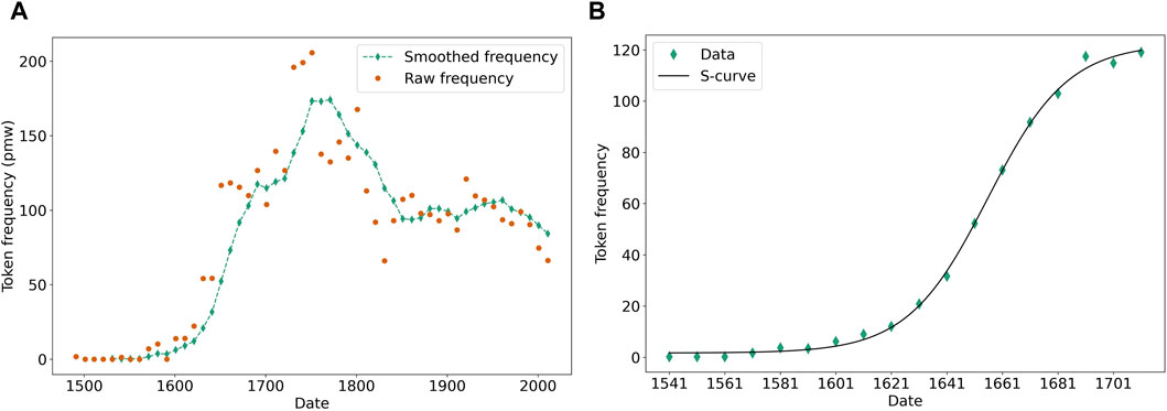
FIGURE 1. Token frequency of the paraître ADJ construction (A) over the whole corpus, both raw and smoothed over five datapoints; (B) over the selected change episode (smoothed), with the corresponding S-curve fit.

3.1.5 Extracting change episodes

One tricky methodological issue is to automatically detect a change episode. In this study, we decided to keep only one change episode per linguistic form (although several may occur throughout their diachronic history), and proceeded as follows. First, we computed the difference in token frequency for all pairs of data points set five data points away (e.g., f_1601−1610 − f_1551−1560, f_1611−1620 − f_1561−1570, etc.), and picked up the interval associated with the largest difference as a starting point (under the assumption that a change episode is associated with a large increase in token frequency). Then, we extended this interval for both sides up to 10 data points and tried all possible pairs as starting and end points (e.g., if the difference in token frequency between decades 1,551–1,560 and 1,601–1,610 was the largest, we tried everything from 1,451 to 1,460 to 1,551-1,560 as a starting point, and from 1,601 to 1,610 to 1701-1710 as an end point).

The next step is to decide which of these intervals is the most closely associated with the S-curve model. Goodness of fit measures would favor shorter intervals. To circumvent this issue, we compared, for all trial pairs, an S-curve model described by (6) to a third-order polynomial model (therefore of equal complexity in terms of number of parameters), and picked the interval over which the S-curve outperforms the polynomial the most, in terms of the r² of the fit. The rationale is that, if only a fraction of the S-curve pattern is featured, a polynomial model is equally good in that it can reproduce the same shape; if we extend past the S-curve pattern, the polynomial model, being more versatile, will accommodate better the variation that may be found; if the interval focuses on the S-curve pattern strictly, the polynomial model cannot bend enough to capture it closely and the S-curve will be the better model by a wider margin. This solution, however crude, proved consistently efficient over a large array of token frequency time series, even though it tends to extend the selected pattern beyond what a manual selection would pick; e.g., the method will often include a possible decrease after the plateau of the S-curve has been reached, such a decrease being quite pervasive in empirical data (Feltgen et al., 2017). It is nonetheless simple enough and ensures the reproducibility of the analysis. An example of such a change episode selection with the corresponding S-curve fit is given for the construction paraître ADJ in Figure 1B.

3.2 Empirical study

We now study the token frequency profile of 25 forms based on data from the French textual database Frantext (ATILF, 1998), restricted to the seven centuries window 1,321–2020 (such that each decade features at least 5 texts). The complete list of forms can be found in the Supplementary Material. For each of these forms, we identified an S-curve episode to choose a tighter time window (the data otherwise spans 70 decades). On this time window, we computed, besides the token frequency, the type frequency, the corpus prevalence, the diversity, and the prototype entrenchment. For each such quantity, we attempted an S-curve fit and, if conclusive, extracted the corresponding parameters. We also computed their correlation coefficient with the token frequency.

Furthermore, although these different quantities typically vary on different scales, the increase magnitude A can be extracted for each of these variables, provided the S-curve fit is successful. By running a multifactorial regression on the change magnitude of the token frequency, we shall assess which of the three factors (change magnitude of the prototype entrenchment, diversity, and corpus prevalence) explains this change magnitude the best. Finally, we also run a multifactorial regression of the token frequency itself to assess which of our three factors explains the dynamics the best across all changes.

3.2.1 Correlations across variables

For each form, we extracted our five variables (token frequency, type frequency, corpus prevalence, diversity, and prototype entrenchment) over the time period associated with the S-curve-like token frequency increase. These variables are shown in Figure 2 for the paraître ADJ construction. We then computed the correlation of each time series with token frequency, setting the significance threshold at α = 0.05/4 = 0.0125, since we perform four comparisons for each form. It turns out that the correlations between token frequency and the other four variables are significant for all variables, and for each individual form, with one exception: the prevalence of the passive form se faire + Vinf (“to be V-ed”). Indeed, although the token frequency increase is important (from 250 hits per million words to 450 hits per million words), the form was already well established at the beginning of this evolution, and the prevalence was saturated at a value close to 90% of the authors, so it could not increase much past this point. This shows that a widespread form can still be associated with important changes. However, one could point out that the innovative uses associated with the form, which would explain the token frequency increase, had to diffuse over the speakers’ community just as well, and sorting out these uses could certainly help to recover a proper pattern of prevalence increase. However, telling apart the types of the new functional domain from the new types recruited in the former functional domain, typically requires an extensive linguistic analysis. Furthermore, the extension of the construction to a new functional domain may encourage its use overall, including in relation to the former functional domain, so types tying to that domain may increase in frequency as well anyway.

FIGURE 2

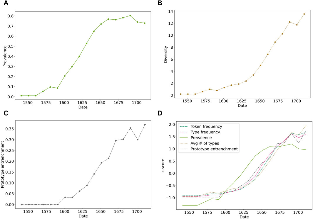
FIGURE 2. Diachronic variations of the paraître ADJ construction. (A) Prevalence (proportion of authors using the form). (B) Diversity (average number of types over the texts where the form is used). (C) Prototype entrenchment (average token frequency of the most frequent type over the texts where the form is used). (D) All three previous quantities, alongside token and type frequencies, z-scored over the time period for better comparison.

Overall, the correlation between these variables is very strong, as evidenced by the very high median values of the Pearson correlation coefficient reported in Figure 3A. The average value is weaker for the prototype entrenchment. This may be a result of the much smaller sample size (since we focus on data from a single type), and of the comparatively larger fluctuations that this smaller size entails. One of the weakest correlations, the one for en marge de, whose prototype is société (literally ’on the margins of society’), is due to one author using it twice in the decade 1841-1850 where the token frequency had not yet taken off and only three authors were using the form, leading to a fairly high prototype entrenchment value (2/3, which is then smoothed out to 0.13 for this decade and the four following ones due to the moving average). This type is then never used before 1921-1930, where it follows the overall trend of the en marge de construction that picks up momentum at this time. Therefore, because of one single fluctuation due to the very limited sample size.

FIGURE 3

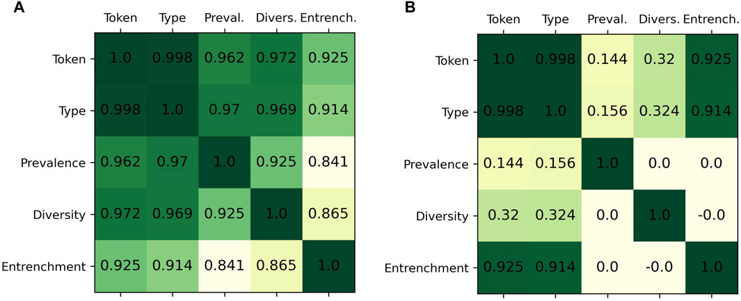
FIGURE 3. Median correlation over 25 linguistic forms between token frequency, type frequency, corpus prevalence, diversity, and prototype entrenchment. (A) standard version (B) with orthogonalization.

That all the three ”components” of the change (corpus prevalence, diversity, and prototype entrenchment) are so closely correlated with one another despite reflecting different features of the dataset hints that they all reflect the same ongoing process. Moreover, we have already argued that there is no way to measure prevalence in the corpus in a way that does not depend on the extent to which individuals use a form, since the latter automatically increases the probability that a given author produces the form at least one and therefore becomes accounted for in the corpus prevalence. The same goes for diversity: if individual types are used more overall, then they have a greater chance to register in the data. Prototype entrenchment, being by construction a direct measure of how much a chosen type may be used by an individual that knows the form, does not depend on the probability that the author knows the form (it is conditioned by it), nor on the diversity of types (it focuses on only one type). Here, all three measures are closely correlated, with each other on the one hand and with the token frequency on the other hand. A likely explanation of this fact is thus that they all reflect this entrenchment.

To confirm this, we performed a Gram-Schmidt orthogonalization to extract the effect of entrenchment out of both diversity and corpus prevalence, and of diversity from corpus prevalence (note: we orthogonalized the z-scored variables to ensure a 0 Pearson’s correlation score). The associated correlation matrix is shown in Figure 3B. In this case, only 8 forms have a diversity that correlates significantly with token frequency, and none have a corpus prevalence that correlates significantly with token frequency. In short, there is no component of prevalence independent of diversity and prototype entrenchment that correlates with the diachronic profile of the token frequency.

3.2.2 Factors of token frequency

To go beyond these individual correlations, we assess which of the three variables weighs the most in predicting the token frequency. To do so, we pooled, on the one hand, the token frequencies of each construction (z-scored over the change interval), and on the other hand, the corpus prevalence, the diversity, and the prototype entrenchment of each construction (z-scored over the change interval as well). We then performed a multivariate linear regression fit of the pooled token frequency (all the variables were z-scored again). The weights associated with each of these three factors are then all significant (respectively 0.46, 0.45, and 0.10, all with p < 0.001). The model then explains 94% of the variance of the token frequency. If we orthogonalize the pooled corpus prevalence, diversity, and prototype entrenchment for the regression, we obtain respective weights of 0.23, 0.40, and 0.85 (all significant with p < 0.001, mapping to a percentage of explained variance of 5%, 16%, and 72%.

We then did the same thing, using the orthogonalized versions of the corpus prevalence and the diversity when pooling the data. Here again, the weights of all three factors were highly significant (respectively 0.21, 0.36, and 0.86, all with p < 0.001), leading to 5%, 13%, and 74% of variance explained, for a total of 91% explained variance. Therefore the two procedures lead to very similar results.

We considered varying the orthogonalization order for the first of these two analyses, and the corresponding results are displayed in Table 1. It is worth noting that, even entrenchment remains significant, its explanatory power is largely depleted when it comes last in the orthogonalization procedure, with an explained variance dropping below 1%. This is in line with the design of these variables, in the sense that prototype entrenchment is only supposed to reflect entrenchment, while the other two variables reflect both entrenchment and either the domain of use or the actual prevalence. Diversity independently accounts for 4% of the variance, corpus prevalence for 5% of it, prototype entrenchment for 0%; 1% of explained variance is shared between corpus prevalence and prototype entrenchment to the exclusion of diversity, 12% between corpus prevalence and diversity, 2% between entrenchment and corpus prevalence. Finally, the remaining 68% of variance (the bulk of it) is distributed across the three variables depending on the orthogonalization order. Since we assume that these three variables all share a common sensitivity to entrenchment (a view reinforced by the very low share of explained variance explained by prototype entrenchment alone), this factor seems to be the main drive of token frequency.

TABLE 1

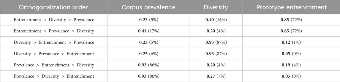
TABLE 1. Weights of the orthogonalized, z-scored pooled corpus prevalence, diversity, and prototype entrenchment, in the regression of the z-scored pooled token frequency, depending on the orthogonalization order. Percentage of explained variance in parentheses. Significant regressors in bold.

The key teaching of this analysis is that, if we first try to explain as much as the token frequency based on prototype entrenchment, we find a very high score (above 70%). The diversity and the prevalence don’t explain much more, yet they both improve the model. This is comforting, as we do expect all of these factors to contribute to the variations in token frequency (that is, at equal entrenchment and equal diversity, a greater corpus prevalence should indicate a greater pervasiveness of the form in the population and therefore drives the token frequency up). However, their independent contribution is marginal compared to that of the prototype entrenchment.

3.2.3 Magnitude of the change

Another interesting variable to consider is the magnitude of the change - the total increase in token frequency. Indeed, not all linguistic changes lead to the same frequency increase. If we assume change to be mostly driven by prevalence, we should be able to translate a percentage of adopters increase to a corresponding token frequency increase. However, the token frequency disparities among linguistic forms are wide, even though a large number of these forms can be assumed to be part of the linguistic knowledge shared over the whole community. Since the increase in token frequency varies from one form to the next, it suggests that token frequency reflects something more than the spreading of the form over the community. Therefore, the diffusion process that the S-curve in token frequency records may not be a social diffusion only, but also a lexical diffusion, or a structural diffusion, as per our three hypotheses for change.

To test this idea, we fitted each time series with an S-curve over the selected time period and recovered the parameter A (Eq. 6). Not all time series for all linguistic forms could be fitted with an S-curve: the diversity variable for en passe de + Vinf, both the prevalence and diversity for se faire + Vinf, the prevalence for se voir + Vinf, and the prototype entrenchment for dans l’espoir de + Vinf, porter à + Vinf, quasiment + ADJ, and une foule de + N. Therefore, we were left with only 18 linguistic forms.

Over these, we performed a multivariate regression of the z-scored A parameter found for the token frequency with the z-scored A parameter found for the other three variables (corpus prevalence, diversity, prototype entrenchment). We find weights respectively equal to 0.09 (p = 0.28), 0.91 (p < 0.001), and 0.02 (p = 0.79). In other terms, only the magnitude of the increase in diversity is predictive of the magnitude of the increase in token frequency. The model explains 95% of the variance in magnitude across the 18 forms.

Since these three variables are highly correlated, we orthogonalized them according to a Gram-Schmidt process, taking prototype entrenchment as a reference, then diversity, and then corpus prevalence, due to the causal asymmetrical relationship between the three. The regression coefficients for corpus prevalence, diversity, and prototype entrenchment are respectively equal to 0.07 (p = 0.28), 0.95 (p < 0.001), and 0.22 (p = 0.002), accounting for 0%, 89%, and 5% of the variance respectively.

Although this orthogonalization is the one that makes the most sense with respect to how these variables were designed, we tested different orthogonalization orders as displayed in Table 2. The diversity factor is always the most important one, and its weight is always significant. The entrenchment factor is only significant if taken as the reference factor, which is expected since the other two factors depend as well on entrenchment, making it redundant. More surprisingly, the corpus prevalence is a good predictor if it comes before diversity; this means that the final value of the corpus prevalence depends more on the extent of the domain of use, than on the extent of the entrenchment. However, if both prototype entrenchment and diversity are factored out of corpus prevalence, it has no predictive power on the magnitude of the token frequency increase.

TABLE 2

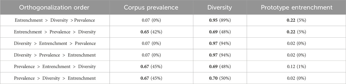
TABLE 2. Weights of the orthogonalized, z-scored magnitudes of the increase in corpus prevalence, diversity, and prototype entrenchment, in the regression of the z-scored magnitude of token frequency increase, depending on the orthogonalization order. Percentage of explained variance in parentheses. Significant regressors in bold.

These results are both consistent with the meaning of these variables, and surprising in some measure. They are consistent in the sense that diversity plays a pivotal role, and diversity aims at capturing the extent of the lexical domain over which these constructions apply. If the domain of use is seen as the ”limiting” factor of token frequency (the entrenchment ultimately unfolds over this particular domain of use), then it is consistent that diversity predicts best the overall increase, with 89% of explained variance even when entrenchment is factored out. This also means that the lexical domain of the construction closely maps to its functional domain of use understood in a broader sense. The results are surprising, however, in that the magnitude of entrenchment of the prototype plays a weak role in determining the final frequency. Yet, not all linguistic forms under change are schematic: discourse markers, in particular, being fixed and extra-clausal, typically have an unrestricted lexical domain, and diversity could not be defined for these forms. In that case, the average individual entrenchment (how much authors who know the marker use it on average) would be the only way to access the extent of the functional domain. Since entrenchment should determine the extent of token frequency in these cases, it is unexpected that it plays a negligible role in determining the extent of use of schematic constructions.

The marginal role of the prevalence, which does not significantly predict the magnitude of the token frequency independently of the entrenchment and the diversity contributions, is not much surprising: most forms are expected to spread over the whole community eventually, so the end point of the process of social diffusion should be roughly the same for all linguistic forms. One exception could be that of a form that acts as an identity marker of a sub-community, but none of the forms under study here are marked sociolinguistically. It could be interesting to perform the same analysis over forms with varying markedness, in which case we would expect an effect of corpus prevalence on the increase in token frequency.

To sum up this series of results, the picture that transpires from our results is that diachronic changes in token frequency of a form appear to mostly reflect a dynamical entrenchment process over a domain of use predominantly shaped by the lexical diversity of the construction.

4 The emergence of a local structure

The conclusion of the previous section is, to some extent, conflicted: on the one hand, prototype entrenchment explains a large part of the token frequency by itself (72%), on the other hand, the magnitude of the overall change in use seems largely determined by the increase in diversity (89% once prototype entrenchment is factored out). To resolve this discrepancy, we investigate with more scrutiny the emergence of these schematic constructions, with an emphasis on their structural organization. Our hypothesis is the following: the rise of schematic constructions is characterized by an initial ”trigger”, that is, a semantic expansion sanctioned by the system, that corresponds to the transition from a bridging context to a switch context in Heine’s account of grammaticalization (Heine, 2002). This semantic expansion sets a priori the extent of the domain of use, over which the construction gets progressively entrenched. In this way, the diachronic dynamics is that of entrenchment, but the magnitude of the change is driven by the extension of the domain, proxied by the diversity of types compatible with the use of the construction.

This view would go against a picture of linguistic change where the process is driven by an increase in type frequency (Smith, 2001), that is, where the change diffuses over an increasingly large domain, gaining new compatible types over time. Our view is that the whole domain becomes entirely available, but gets progressively sampled with an increasing number of tokens, therefore revealing new types. This view is supported by empirical evidence: distributional semantic plots associated with the rise of the way construction for instance show that the early types are scattered all across the semantic domain covered by the construction (Perek, 2018). The new types appear because the domain becomes more densely populated with tokens, not because the form extends to a new domain. Of course, this view does not preclude that a domain extension is possible in practice. We solely argue that a single S-curve corresponds to one semantic trigger, and therefore displays how the construction is taking over the associated domain of use. Multiple S-curves can theoretically occur and even overlap if a new trigger takes place before the entrenchment over the first domain has ended.

In this section, we provide evidence that shows the consistency of this scenario, starting with the hypothesis that the individual fillers’ token frequencies of a schematic construction collectively obey a diachronically stable Zipf-Mandelbrot distribution. Then, focusing on one well-behaving construction, we show that the diachronic frequency profiles of each individual filler are compatible with a sampling of the overall Zipf-Mandelbrot.

4.1 Zipf-Mandelbrot structure

As we have argued, language change is not only a social affair: it implies a stronger degree of entrenchment in use, which then becomes reflected, for schematic constructions, in an increased number of different types hosted by the construction. What is more, this open schema is structured: the types that appear are not random, they are highly idiosyncratic to the construction (Goldberg et al., 2004); e.g., the near-synonyms pratiquement and quasiment, both meaning “almost”, do not combine with the same adjectives: their top 10 fillers have only three fillers in common. As we will detail in this section, they are hierarchically organized, obeying a Zipf-Mandelbrot law at the scale of the construction, and a diachronally stable ranking among types.

This is interesting for two reasons. First, it hints at a dimension of complexity in language change that has remained largely ignored by empirical scholars so far, Zipf’s law being typically applied to language as a whole in this tradition. Second, it explains how type diversity can be driven by prototype entrenchment: since the construction is associated with a stable, hierarchical organization, for the frequency spectrum to be broadened, the leading types must become more entrenched.

In Construction Grammar, the intuition that schematic constructions are tightly selective with respect to their fillers, in agreement with a Zipf’s law pattern, has been formulated early on (Goldberg et al., 2004), and empirically confirmed by Ellis and Ferreira-Junior (2009). In parallel, the study of both morphological productivity (Baroni, 2005) and syntactic productivity (Zeldes, 2012) has also led to describe the fillers’ frequencies distribution as a Zipf-Mandelbrot distribution. Furthermore, it has been observed that the corresponding ranking is stable over the acquisition period (Ellis and Larsen-Freeman, 2009) and over the emergence process of a new form (Feltgen, 2022a).

The Zipf-Mandelbrot law states that if the different types of a construction are ranked according to their frequency, then the relationship between the rank r of an item and its frequency f_r is given by:

$f_r=\frac{A}{{\left(r+b\right)}^{\alpha }}(7)$

In practice, fitting the law is problematic, especially since many items have the same empirical frequency (typically 1, 2 or 3 hits), as predicted by the law itself (Evert, 2004), although this issue may be addressed with a cut-off of the items with lowest frequency (Izsák, 2006). Furthermore, the parameter fit heavily depends on sample size, especially for small sample sizes (Baayen, 2001; Evert and Baroni, 2005).

As a result, relying on a Zipf-Mandelbrot fit of each decade to assess the diachronic robustness of the construction’s organization is not warranted. To circumvent this issue, we rather show that the Zipf-Mandelbrot distribution holds for the construction schema over the whole time period (by pooling together all of the associated data), and that the ranking of the constructions’ fillers is stable over the change episode.

4.1.1 Zipf-Mandelbrot overall fit

Our data, for each of the 25 linguistic forms, is the collection of all tokens covered by the change episode, including those from the four preceding decades as they are accounted for in the moving average of the token frequency. To fit the data, we used the curve_fit algorithm from the scipy library in Python 3, fitting the logarithm of the frequency rather than the frequency itself. This method relies on a least squares minimization, which is criticized by Izsák (2006). Similarly, Koplenig (2018) argues for the maximum likelihood evaluation (MLE) method. The main issue of this method is that it crucially hinges on the chosen low-frequency cut-off, especially for the small sample sizes associated with historical data. Moreover, a cut-off would leave us with too few items in some cases, and would probably need to be adjusted on a case-by-case basis. This is the reason why we favored a more naive fit of the log-transformed frequency, except that instead of applying a cut-off to exclude low-frequency items, we rather consider the minimum rank for items sharing the same frequency (for instance, if items ranked 34, 35, and 36 all have frequency 2, and items ranked 37 to the last have frequency 1, we only keep one data point (34, 2), as well as a datapoint (37, 1) for all the hapax legomena). To ensure the reliability of this method, we randomly generated small sample size data from Zipf-Mandelbrot distributions to check whether the different methods (Koplenig’s MLE, Evert’s fit of the frequency spectrum 2004, and a curve fit of the log-transformed frequency) can recover the distribution’s parameters, and found that the straight fit of the log-transformed frequency works adequately (it is less accurate than Evert’s method but more consistent). Importantly, the superiority of the MLE method has been established with respect to the asymptotic regime of these distributions (Corral et al., 2020), which does not apply here, and one of the major issues with the least-squares fit is the inconsistencies due to binning data, which we do not do here thanks to our trick.

The Zipf-Mandelbrot fit is overall excellent for all linguistic forms. The r² of the corresponding fit ranges from 0.928 to 0.995, with a mean of 0.978 and an interquartile range between 0.97 and 0.99. The Inter Quartile Range for both parameters α and b are respectively [0.91; 1.30] and [0.35; 3.77].

4.1.2 A stable ranking

To assess the stability of the ranking, for each individual linguistic form, we selected the 10 items whose frequency increases the most over the whole episode of change. Next, we recovered the ranking of each of these items over each window of 50 years covered by the S-curve pattern, sliding that window with a one-decade step over the whole change episode, and we computed the Spearman correlation coefficient between these ranks and the overall ranking. Next, we compared this value (for each 50-year window) with a distribution of Spearman correlation values between the overall ranking and 1,000 random samples from the whole pool of tokens, of a size matching that of the number of the tokens in the 50-year window. We show in Figure 4 the evolution of that correlation over the different decades for two examples, obliger à + Vinf (’to force/to make (something/someone) V′) and tenir à + Vinf (“to care about/to insist on Ving”). The former is an example of a process for which the ranking is not stable over time: on the contrary, the Spearman correlation keeps increasing, which indicates that the ranking has changed significantly during the period of token frequency increase. The latter, on the other hand, is a case where the ranking is diachronically stable over the whole change episode.

FIGURE 4

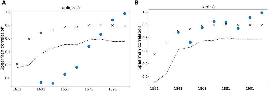
FIGURE 4. Spearman correlation coefficient between the decade-based rankings of the ten most frequent fillers, for (A) the obliger à construction and (B) the tenir à construction. Blue dots shows the correlation between window ranking and overall ranking. This is compared to a distribution of correlation values based on random samples of the whole pool. The mean and the lower 5% limit of this distribution are shown for each window, respectively with a black cross and a black dotted line.

For 17 out of the 25 constructions, the Spearman correlation between the window ranking and the overall ranking is always consistent with a random sampling of the common pool of tokens (that is, above the 5% most uncorrelated values in the distribution). The ranking thus appears to be significantly stable over the duration of the S-curve pattern, at least as soon as the form becomes frequent enough to reliably host a variety of types. Although this result seems to establish quite strongly the diachronic stability of the ranking, it must be considered with caution: for most of the forms, the 10 selected types do not consistently appear in the 50-year windows that make up the change episode. For these windows, the missing fillers have no rank and the Spearman correlation cannot be computed. As a result, some forms are associated with a very low number of data points. If we only keep the forms with at least 5 data points, we are left with 12 forms, and for 6 of them, the Spearman correlation is consistent with a global hierarchy between the types all throughout the change episode.

Besides assessing the stability of the ranking, describing the diachronic behavior of this Spearman correlation offers a tool to witness structural changes in the construction’s organization. Typically, the higher half of the S-curve is associated with a constant ranking, but once the plateau is reached, the ranking starts to fall apart, indicative that the organization structure may not last beyond the S-curve increase. These observations elicit a wealth of questions regarding the stability of a construction’s organization, and the ways by which it may sustain, lose, and regain stability.

4.2 A cohesive evolution of the types

We now turn to the individual evolution of the types by considering their own token frequencies over time, and how these token frequencies relate to the overall token frequency overall. Here we consider the collocate frequencies, that is, we count the occurrences of each of these types in association with the construction; e.g., we consider the token frequencies of apprendre à lire (“to learn to read”), not the frequency of lire (“to read”) overall in the corpus. As such, our purpose here is not to explore the relationship between the overall frequency of the fillers and the time at which they are recruited in the construction.

If the structural organization of the fillers holds over time, then the number of tokens of a given filler found within the construction should scale linearly with the number of tokens of the construction registered so far, fluctuations aside. Moreover, each type should follow a token frequency trajectory akin to that of the construction as a whole. Historical data, however, being limited in size, severely restricts these investigations. For instance, one of our syntactic pattern is the lexical pattern boîte à N (’N box’), which is a daughter construction of a more general schema N à N (tasse à café, planche à pain, etc.). One of the ten selected fillers is pêche, “fishing”. This filler is quite unusual; actually, it appears in only one text in the corpus from 1926, entitled La boîte à pêche, and is referred to numerous times throughout that text. This produces a spurious peak of frequency which is not reflective of the community use. Furthermore, some fillers may have dynamics of their own: the 26th most frequent filler of habituer à Vinf (’to be used to V′) in the frTenTen20 synchronic corpus, évoluer, with the meaning “to move around” or “to navigate” (with respect to a social context), only appears in the late 19th century, when the construction was already established. Another potential cause of disruption of the alleged pattern is internal competition between clusters of fillers (Feltgen, 2022b). For these reasons (both empirical, due to the scarce nature of the data, and theoretical, because different processes of change may interact), a perfectly clean and cohesive bundle of patterns is expected to be rare.

4.2.1 Diachronic consistency of the Zipf-Mandelbrot organization

In the following, we illustrate the cohesive evolution of the fillers for one specific example, the construction habituer à + Vinf. We admittedly chose one that exemplifies the pattern clearly, to emphasize how coherent the picture might be for some constructions, despite the possible cause of disruptions discussed above. First, we fitted in Figure 5A the entirety of the tokens pool associated with the change episode with a Zipf-Mandelbrot distribution, as described above; the fitted parameters are α = 0.99 and b = 4.52, with an r² of 0.994.

FIGURE 5

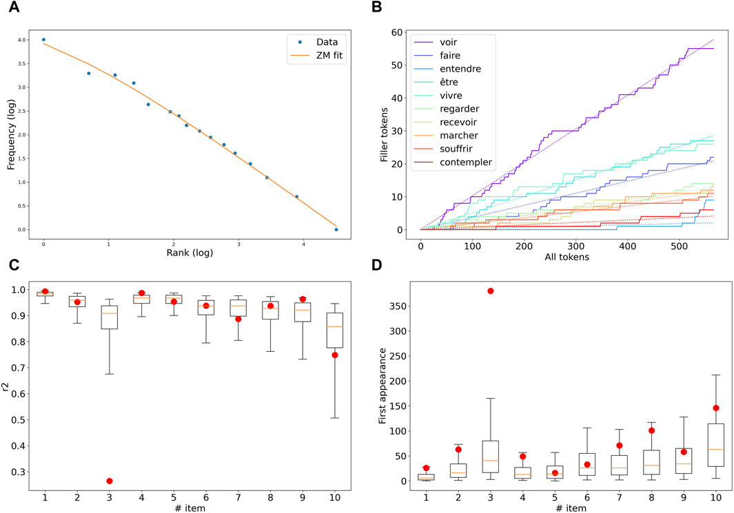
FIGURE 5. Analysis of the schematic organization of the habituer à Vinf construction. (A) Zipf-Mandelbrot fit of the data pooled over the whole change episode. (B) Number of tokens of each of the 10 most frequent fillers as the sequence of tokens goes on chronologically. (C) r² of the linear fit (in red dots) of the token growth curve of each of these 10 fillers, as compared to the distribution of the r² computed from random reshufflings of the sequence. (D) First appearance of each type in the token sequence (red dots) vs. distribution of this first appearance position over 1,000 reshuffled token sequences.

Next, we test whether the growth of the tokens’ share of each filler is on average constant, and therefore whether the tokens’ pool of each filler grows linearly with the total number of tokens of the construction. Crucially, these tokens are accounted for sequentially, in the order of their associated year of occurrence. A constant tokens’ share means that the frequency organization, which we have just shown is well accounted for by a Zipf-Mandelbrot pattern, is robust over time. We then measure the r² of the linear fit of each of the type-specific tokens’ pool growth curve, as seen in Figure 5B. To assess the linearity of these curves, we randomly shuffled the sequence of tokens and produced the same data (the r² of the linear fit of the type-specific tokens’ pool growth as tokens are progressively drawn from the common pool). Since the sequence is now random, the proportion of tokens of any given filler is, on average, constant over the sequence. Therefore, we performed a linear fit on this data as a reference point. We repeated this procedure 1,000 times to compute a distribution of the r² of the linear fit for each filler, and compared the r² linear fit found over the chronologically ordered sequence to that distribution. It appears in Figure 5C that the linear fit is valid for all of the fillers (only one, habituer à entendre, ’to be used to hear’, clearly deviates from its respective distribution).

To assess whether the lexical domain of the construction is gradually extended, or readily available in its entirety from the start, we also consider whether sampling the Zipf-Mandelbrot organization may explain the disparities between the first appearance of each type. The rationale is that low-frequency types have a lower chance of being sampled and therefore appear later on in the sequence. We display in Figure 5D the first appearance ’time’ for each type (in terms of the position in the chronologically ordered sequence of tokens), compared to the distribution of these first appearance times over random shufflings of the sequence. Here again, habituer à entendre deviates from the random distribution for more than two standard deviations, and habituer à faire (’to be used to do’) as well, albeit to a lesser extent. Most of the types (8 out of 10) appear at a time that is consistent with a fixed domain of use.

4.2.2 Individual token frequencies of the types

Finally, we display in Figure 6 the token frequency of each of the ten most frequent fillers over the entirety of the change episode. Since the token frequencies vary widely in magnitude (as expected in a Zipfian distribution), we z-scored these frequencies over the change episode, and we aligned the curves so they would all start at 0 (none of the fillers is attested within the construction prior to the change episode in this case). It appears that all the fillers rise up in frequency over a very limited period of time, simultaneously, and following a curve of more or less the same S-shape once properly rescaled.

FIGURE 6

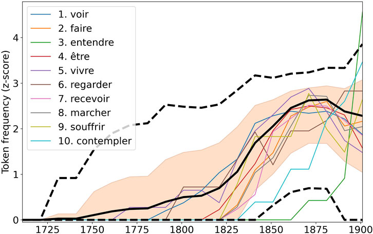
FIGURE 6. Rescaled (through z-scoring and aligning) token frequencies of each of the 10 most frequent fillers, compared to frequency trajectories of random samplings of the overall token pool. The red area indicates a width of the ”bundle” which is below the median deviation from the construction’s token frequency, and the black dotted lines show the threshold associated with the 5% most extreme deviations both above and beyond the construction’s token frequency.

To go beyond visual assessment, we compare this bundle of trajectories with random samplings of the common pool for each decade. For each time window, for each filler, we sample the common pool with a number of tokens matching that of the time window and count the tokens of the filler in that sample, turning then this count into a smoothed token frequency as per our usual procedure. We then compute, for each decade how much these individual trajectories spread above and below the trajectory of the construction as a whole. Since the samples are drawn from the common pool, this gives us the expected behavior when the associated Zipf-Mandelbrot organization is valid throughout the diachronic evolution. We repeat the same for 1,000 samples and build a distribution of this “spreading” value. We then consider whether the fillers are within the average of this spreading, and whether they are within the expected variation of the spreading (we fix the threshold to exclude the 5% most extreme values in both directions separately).

It appears that habituer à entendre appears late and behaves differently than the other forms. The rise of habituer à contempler (’to be used to behold’) is also slightly late (although within the threshold). Otherwise, all the fillers’ token frequencies behave similarly to that of the whole construction. Moreover, two fillers have one point that goes past the median deviation. Therefore, and with the clear exception of habituer à entendre, the whole episode of change appears largely consistent with the overall organization of the construction.

4.2.3 Statistics for the other constructions

How much atypical is this behavior in our assortment of constructions? On average (the average is performed over the 25 constructions), there are 7.4 fillers following a tokens’ pool linear growth (out of 10). For 6 constructions, all of the fillers satisfyingly follow a linear fit. Similarly, the first appearance of 7.12 fillers is consistent with a random sampling, and the whole 10 fillers are consistent with a random sampling for only 2 constructions (which are not among the 6 previous ones). Note that we consider that a “deviation” occurs whenever the r² (or the first appearance time) is more than two standard deviations away from the mean of the random distribution.

Regarding the behavior of the individual token frequencies, on average, 5.2 forms are past the median deviation for at least one time window, but only 1.16 are past the threshold deviation for at least one time window. Three constructions have all of their fillers’ token frequencies within the median deviation, and 7 of them have at least six of these profiles within the median deviation (habituer à is therefore among the 28% ’most consistent’ constructions). Twelve forms have all of their fillers’ trajectories within the deviation threshold, and 17, like habituer à, have only one filler that goes past this threshold.

If we now consider the percentage of points that go past the median deviation (resp. Past the threshold deviation), we find an average percentage of 9% (resp. 1%) deviating points. These numbers, however, should not overshadow the fact that, for some fillers, the deviation is consistent over several successive data points, which has few chances to happen due to random fluctuations. For three constructions, 4 or 5 fillers are past the threshold (all 22 other constructions have no more than 2 fillers that get past the threshold). These are boîte à N, se faire Vinf and pratiquement. In these cases, it is likely that a lexical diffusion of some sort is at work.

4.3 Discussion

We tried to empirically distinguish whether the organization holds from the very beginning of the change and gets entrenched as such, or whether it emerges diachronically as a process. We now briefly discuss which processes might lead to these two outcomes. We showed that, for some constructions at least, there is no need to posit a process of domain extension (of lexical diffusion), and that an entrenchment dynamics alone over a set domain already accounts for the collective behavior of the individual types.

In the first view, we need to explain how a semantic expansion can lead to a predefined domain of use. To explain this, we may think of the meaning territory as an interconnected network of sites (minimal domains), with connecting strangleholds in between clusters of sites. These strangleholds are typically hard to cross and can hold off a form for decades. If the stranglehold is past though, a whole domain becomes accessible and the form can spread quickly all over it. Therefore, there can be a correspondence between a specific semantic expansion, and a domain over which to diffuse. However, this view also holds that the diffusion is near-instantaneous, while the entrenchment is typically much slower, and this probably poses some tight constraints on the semantic network organization.

Alternatively, the constructional structure may be the result of an unfolding process, unpredictable at the start. For instance, the Adjacent Possible Model (Tria et al., 2014) simulates the process of vocabulary growth via an urn model relying on two mechanics: reinforcement and expansion into a space of possibilities. Concretely, whenever a token is drawn, the corresponding type gets reinforced by the addition of more tokens of this type; if, however, this type is new to the sequence of drawn tokens, additional tokens corresponding to novel types are also added into the urn. This model adequately captures the features of a Zipf-Mandelbrot organization (Tria et al., 2018). Due to the reinforcement mechanic, the items that appear first have a greater chance of becoming dominant.

These two scenarios, however, differ in the role played by token frequency. In the Adjacent Possible Scenario, the growth goes on indefinitely: the token frequency dynamics is therefore a parallel, independent process to that of the vocabulary diversification. In the schema emergence scenario, the pattern in token frequency could be explained as the linguistic form ”fills in” the language use niche that is associated with the schema, which can result in an S-curve (Feltgen et al., 2017).

More likely though, a mixture of these two scenarios may happen, with part of the organization being shaped by the semantic reanalysis that triggers the S-curve, and part of it being driven by an ongoing process of further analogization, of the kind empirically evidenced by (Perek, 2016), provided that this analogization cannot be explained by a Herdan-driven side-effect of the entrenchment in token frequency of the construction as a whole.

5 Conclusion

Is language change chiefly a social diffusion affair? Yes, in the sense that no language change could unfold without a proper social dynamics to support it and spread it over the community of speakers. No, in the sense that, if we subtract the effects of entrenchment and lexical diversification from empirical estimates of prevalence, then the latter factor independently explains very little of the dynamics and features of language use, as apprehended through token frequency rise. However, this result may well hinge on the specific nature of the linguistic items we considered in this paper, these being schematic constructions with a functional use. We may expect a greater sensitivity to prevalence with, for instance, discourse markers, which are typically more noticeable and more gradient in their sociolinguistic marking (Foolen, 2011). The method we offered in this paper could test such a hypothesis.

Our paper shows that the rise in token frequency, for the kind of constructions we studied, can primarily be interpreted as reflecting the entrenchment in use of the form over a functional domain. The entrenchment process is the best predictor of the token frequency dynamics, while the increase in diversity of use (the proxy that we used to appreciate the extent of the functional domain) is the best predictor of the magnitude of the rise. Furthermore, the constructions that we analyzed feature an open slot (or schema) hosting a diversity of fillers known as types. Focusing on the social dynamics overshadows the complex changes ongoing on the level of that schema. These dynamics involve a robust Zipf-Mandelbrot organization over the duration of the S-curve pattern in token frequency change, reflected in the cohesive evolution of the individual types.

The chief argument of this paper is not to belittle in any way the accomplishments and the research potential of language change studied, measured, and modeled from a social perspective. Our goal was to highlight that there exists a whole research venture besides it, offered by the study of the complex organization that emerges through the rise of new, schematic constructions, and which structures language at their own scale. This structure seems to obey some key regularities and raises a wealth of questions that are ripe for a more extensive empirically-driven investigation.

Data availability statement

The data analyzed in this study is subject to the following licenses/restrictions: The data has been extracted from the Frantext database which is subject to copyright restrictions. Datasets free from copyright contents (raw token counts) and data analysis Python scripts will be made available in the Trolling repository after acceptance. These datasets will be freely available should be directed to https://dataverse.no/dataverse/trolling.

Author contributions

QF: Conceptualization, Data curation, Formal Analysis, Investigation, Methodology, Project administration, Writing–original draft, Writing–review and editing.

Funding

The author(s) declare financial support was received for the research, authorship, and/or publication of this article. The author acknowledges a postdoctoral research grant from Ghent University: BOF.PDO.2022.0001.01.

Acknowledgments

This is a short text to acknowledge the contributions of specific colleagues, institutions, or agencies that aided the efforts of the authors. I sincerely thank the three reviewers for their precious and constructive input to this work.

Conflict of interest

The author declares that the research was conducted in the absence of any commercial or financial relationships that could be construed as a potential conflict of interest.

Publisher’s note

All claims expressed in this article are solely those of the authors and do not necessarily represent those of their affiliated organizations, or those of the publisher, the editors and the reviewers. Any product that may be evaluated in this article, or claim that may be made by its manufacturer, is not guaranteed or endorsed by the publisher.

Supplementary material

The Supplementary Material for this article can be found online at: https://www.frontiersin.org/articles/10.3389/fcpxs.2024.1327425/full#supplementary-material

References

Adelman, J. S., Brown, G. D., and Quesada, J. F. (2006). Contextual diversity, not word frequency, determines word-naming and lexical decision times. Psychol. Sci. 17, 814–823. doi:10.1111/j.1467-9280.2006.01787.x

PubMed Abstract | CrossRef Full Text | Google Scholar

Aitchison, J. (2012). Language change: progress or decay? Fourth Edition. Cambridge: Cambridge University Press.

Google Scholar

Amato, R., Lacasa, L., Díaz-Guilera, A., and Baronchelli, A. (2018). The dynamics of norm change in the cultural evolution of language. Proc. Natl. Acad. Sci. 115, 8260–8265. doi:10.1073/pnas.1721059115

PubMed Abstract | CrossRef Full Text | Google Scholar

Anthonissen, L., and Petré, P. (2019). Grammaticalization and the linguistic individual: new avenues in lifespan research. Linguist. Vanguard 5, 20180037. doi:10.1515/lingvan-2018-0037

CrossRef Full Text | Google Scholar

ATILF (1998). Atilf. base textuelle frantext.

Google Scholar

Baayen, R. H. (2001). Word frequency distributions. Dordrecht: Kluwer Academic Publishers.

Google Scholar

Bailey, G., Wikle, T., Tillery, J., and Sand, L. (1993). Some patterns of linguistic diffusion. Lang. Var. change 5, 359–390. doi:10.1017/s095439450000154x

CrossRef Full Text | Google Scholar

Baronchelli, A., Gong, T., Puglisi, A., and Loreto, V. (2010). Modeling the emergence of universality in color naming patterns. Proc. Natl. Acad. Sci. 107, 2403–2407. doi:10.1073/pnas.0908533107

PubMed Abstract | CrossRef Full Text | Google Scholar

Baroni, M. (2005). “Distributions in text,” in Corpus linguistics: an international handbook. Berlin: (Mouton de Gruyter), 803–822.

Google Scholar

Baxter, G. J., Blythe, R. A., Croft, W., and McKane, A. J. (2006). Utterance selection model of language change. Phys. Rev. E 73, 046118. doi:10.1103/physreve.73.046118

PubMed Abstract | CrossRef Full Text | Google Scholar

Bickerton, D. (1975). Dynamics of a creole system. Cambridge: Cambridge University Press.

Google Scholar

Bisang, W. (2015). Hidden complexity–the neglected side of complexity and its implications. Linguist. Vanguard 1, 177–187. doi:10.1515/lingvan-2014-1014

CrossRef Full Text | Google Scholar

Blythe, R. A., and Croft, W. (2012). S-curves and the mechanisms of propagation in language change. Language 88, 269–304. doi:10.1353/lan.2012.0027

CrossRef Full Text | Google Scholar

Brysbaert, M., Stevens, M., Mandera, P., and Keuleers, E. (2016). How many words do we know? practical estimates of vocabulary size dependent on word definition, the degree of language input and the participant’s age. Front. Psychol. 7, 1116. doi:10.3389/fpsyg.2016.01116

PubMed Abstract | CrossRef Full Text | Google Scholar

Chambers, J. K. (1990). The Canada-us border as a vanishing isogloss: the evidence of chesterfield. J. Engl. Linguistics 23, 155–166. doi:10.1177/007542429002300113

CrossRef Full Text | Google Scholar

Chen, M. Y., and Wang, W. S. Y. (1975). Sound change: actuation and implementation. Language 51, 255–281. doi:10.2307/412854

CrossRef Full Text | Google Scholar

Corral, Á., Serra, I., and Ferrer-i Cancho, R. (2020). Distinct flavors of zipf’s law and its maximum likelihood fitting: rank-size and size-distribution representations. Phys. Rev. E 102, 052113. doi:10.1103/physreve.102.052113

PubMed Abstract | CrossRef Full Text | Google Scholar

Coulmont, B., Supervie, V., and Breban, R. (2016). The diffusion dynamics of choice: from durable goods markets to fashion first names. Complexity 21, 362–369. doi:10.1002/cplx.21748

CrossRef Full Text | Google Scholar

Dall’Asta, L., Baronchelli, A., Barrat, A., and Loreto, V. (2006). Agreement dynamics on small-world networks. Europhys Lett. 73, 969–975. doi:10.1209/epl/i2005-10481-7

CrossRef Full Text | Google Scholar

Desagulier, G. (2022). Changes in the midst of a construction network: a diachronic construction grammar approach to complex prepositions denoting internal location. Cogn. Linguist. 33, 339–386. doi:10.1515/cog-2021-0128

CrossRef Full Text | Google Scholar

Ellis, N. C., and Ferreira-Junior, F. (2009). Construction learning as a function of frequency, frequency distribution, and function. Mod. Lang. J. 93, 370–385. doi:10.1111/j.1540-4781.2009.00896.x

CrossRef Full Text | Google Scholar

Ellis, N. C., and Larsen-Freeman, D. (2009). Constructing a second language: analyses and computational simulations of the emergence of linguistic constructions from usage. Lang. Learn. 59, 90–125. doi:10.1111/j.1467-9922.2009.00537.x

CrossRef Full Text | Google Scholar

Ellis, N. C., O’Donnell, M. B., and Römer, U. (2014). “Does language zipf right along?,” in Measured language: quantitative studies of acquisition, assessment, and variation. Editors J. Connor-Linton, and L. Wander Amoroso (Washington DC: Georgetown University Press), 33–50.

Google Scholar

Evert, S. (2004). Le poids des mots (JADT vol.1) Actes des 7es Journées internationales d’analyse statistique des données textuelles. Editors Gérald Purnelle, Cédrick Fairon, and Anne Dister Louvain: Presses Universitaires de Louvain, 411–422.

Google Scholar

Evert, S., and Baroni, M. (2005). “Testing the extrapolation quality of word frequency models,” in Proceedings of Corpus Linguistics.

Google Scholar

Fagard, B., and Combettes, B. (2013). De en à dans, un simple remplacement? une étude diachronique. Lang. française 178, 93–115. doi:10.3917/lf.178.0093

CrossRef Full Text | Google Scholar

Feltgen, Q. (2020). Diachronic emergence of zipf-like patterns in construction-specific frequency distributions: a quantitative study of the way too construction. Lexis. J. Engl. Lexicology. doi:10.4000/lexis.4968

CrossRef Full Text | Google Scholar

Feltgen, Q. (2022a). Ce que les variations de fréquence nous apprennent des changements linguistiques: le cas de la construction en plein n. Lang. française 215, 61–80. doi:10.3917/lf.215.0061

CrossRef Full Text | Google Scholar

Feltgen, Q. (2022b). “From qualifiers to quantifiers: semantic shift at the paradigm level,” in 3rd International Workshop on Computational Approaches to Historical Language Change (LChange 2022). (Stroudsburg, PA: Association for Computational Linguistics), 44–53.

CrossRef Full Text | Google Scholar

Feltgen, Q., Fagard, B., and Nadal, J.-P. (2017). Frequency patterns of semantic change: corpus-based evidence of a near-critical dynamics in language change. R. Soc. open Sci. 4, 170830. doi:10.1098/rsos.170830

PubMed Abstract | CrossRef Full Text | Google Scholar

Fonteyn, L., and Nini, A. (2020). Individuality in syntactic variation: an investigation of the seventeenth-century gerund alternation. Cogn. Linguist. 31, 279–308. doi:10.1515/cog-2019-0040

CrossRef Full Text | Google Scholar

Foolen, A. (2011). “Pragmatic markers in a sociopragmatic perspective,” in Pragmatics of society. Editors G. Andersen, and K. Aijmer Berlin/Boston: (Walter de Gruyter), 217–282. (Mouton Berlín).

CrossRef Full Text | Google Scholar

Gardner, M. H., Denis, D., Brook, M., and Tagliamonte, S. A. (2020). Be like and the constant rate effect: from the bottom to the top of the s-curve. Engl. Lang. Linguistics 25, 281–324. doi:10.1017/s1360674320000076

CrossRef Full Text | Google Scholar

Ghanbarnejad, F., Gerlach, M., Miotto, J. M., and Altmann, E. G. (2014). Extracting information from s-curves of language change. J. R. Soc. Interface 11, 20141044. doi:10.1098/rsif.2014.1044

PubMed Abstract | CrossRef Full Text | Google Scholar

Goldberg, A. E., Casenhiser, D. M., and Sethuraman, N. (2004). Learning argument structure generalizations. Cogn. Linguist. 15, 289–316. doi:10.1515/cogl.2004.011

CrossRef Full Text | Google Scholar

Gries, S. T. (2013). Sources of variability relevant to the cognitive sociolinguist, and corpus-as well as psycholinguistic methods and notions to handle them. J. Pragmat. 52, 5–16. doi:10.1016/j.pragma.2012.12.011

CrossRef Full Text | Google Scholar

Hartmann, S., and Ungerer, T. (2023). Attack of the snowclones: a corpus-based analysis of extravagant formulaic patterns. J. Linguistics, 1–36. doi:10.1017/s0022226723000117

CrossRef Full Text | Google Scholar

Heine, B. (1997). Pos-session. Cognitive sources, forces, and grammaticalization. Cambridge: Cambridge University Press.

Google Scholar

Heine, B. (2002). “On the role of context in grammaticalization,” in New reflections on grammaticalization. Editors I. Wilscher, and G. Diewald (Amsterdam/Phildalphia: John Benjamins), 83–101.

CrossRef Full Text | Google Scholar

Heine, B., and Kuteva, T. (2002). World lexicon of grammaticalization. Cambridge: Cambridge University Press.

Google Scholar

Herdan, G. (1960). Type-token mathematics: a textbook of mathematical linguistics. The Hague: S-Gravenhage: Mouton and Co.

Google Scholar

Himmelmann, N. P. (2004). “Lexicalization and grammaticization: opposite or orthogonal?,” in What makes grammaticalization? a look from its fringes and its components (Berlin/New York: Mouton De Gruyter), 21–42.

CrossRef Full Text | Google Scholar

Izsák, J. (2006). Some practical aspects of fitting and testing the zipf-mandelbrot model: a short essay. Scientometrics 67, 107–120. doi:10.1556/scient.67.2006.1.7

CrossRef Full Text | Google Scholar

Johnson, L. (1976). A rate of change index for language. Lang. Soc. 5, 165–172. doi:10.1017/s0047404500007004

CrossRef Full Text | Google Scholar

Kirby, S., and Hurford, J. R. (2002). “The emergence of linguistic structure: an overview of the iterated learning model,” in Simulating the evolution of language (London: Springer), 121–147.

CrossRef Full Text | Google Scholar

Koplenig, A. (2018). Using the parameters of the zipf–mandelbrot law to measure diachronic lexical, syntactical and stylistic changes–a large-scale corpus analysis. Corpus Linguistics Linguistic Theory 14, 1–34. doi:10.1515/cllt-2014-0049

CrossRef Full Text | Google Scholar

Kroch, A. S. (1989). Reflexes of grammar in patterns of language change. Lang. Var. change 1, 199–244. doi:10.1017/s0954394500000168

CrossRef Full Text | Google Scholar

Krug, M. (2000). Emerging English modals: a corpus-based study of grammaticalization. Berlin: Mouton de Gruyter.

Google Scholar

Langacker, R. (2008). Cognitive grammar: a basic introduction. New York: Oxford University Press, 16–17.

Google Scholar

Loreto, V., Baronchelli, A., Mukherjee, A., Puglisi, A., and Tria, F. (2011). Statistical physics of language dynamics. J. Stat. Mech. Theory Exp. 2011, P04006. doi:10.1088/1742-5468/2011/04/p04006

CrossRef Full Text | Google Scholar

Lü, L., Zhang, Z.-K., and Zhou, T. (2010). Zipf’s law leads to heaps’ law: analyzing their relation in finite-size systems. PloS one 5, e14139. doi:10.1371/journal.pone.0014139

PubMed Abstract | CrossRef Full Text | Google Scholar

Mair, C. (2004). “Corpus linguistics and grammaticalisation theory: statistics, frequencies, and beyond,” in Corpus approaches to grammaticalization in English. Editors H. Lindquist, and C. Mair (Amsterdam/Phildalphia: John Benjamins), 121–150.

CrossRef Full Text | Google Scholar

Maybaum, R. (2013). Language change as a social process: diffusion patterns of lexical innovations in twitter. Annu. Meet. Berkeley Linguistics Soc. 39, 152–166. doi:10.3765/bls.v39i1.3877

CrossRef Full Text | Google Scholar

Michard, Q., and Bouchaud, J.-P. (2005). Theory of collective opinion shifts: from smooth trends to abrupt swings. Eur. Phys. J. B 47, 151–159. doi:10.1140/epjb/e2005-00307-0

CrossRef Full Text | Google Scholar

Michaud, J. (2020). “Modelling opinion dynamics and language change: two faces of the same coin,” in Complex networks and their applications VIII: volume 2 proceedings of the eighth international conference on complex networks and their applications COMPLEX NETWORKS 2019 8 (Springer), 305–315.

CrossRef Full Text | Google Scholar

Mühlenbernd, R., and Quinley, J. (2017). Language change and network games. Lang. Linguistics Compass 11, e12235. doi:10.1111/lnc3.12235

CrossRef Full Text | Google Scholar

Nettle, D. (1999). Using social impact theory to simulate language change. Lingua 108, 95–117. doi:10.1016/s0024-3841(98)00046-1

CrossRef Full Text | Google Scholar

Nevalainen, T. (2015). “Descriptive adequacy of the s-curve model in diachronic studies of language change,” in Studies in variation, contacts and change in English, 16.

Google Scholar

Ogura, M. (2012). “The timing of language change,” in The handbook of historical sociolinguistics. Editors J. M. Hernández-Campoy, and J. C. Conde-Silvestre (Oxford: Wiley-Blackwell), 427–450.

CrossRef Full Text | Google Scholar

Perek, F. (2016). Using distributional semantics to study syntactic productivity in diachrony: a case study. Linguistics 54, 149–188. doi:10.1515/ling-2015-0043

CrossRef Full Text | Google Scholar

Perek, F. (2018). Recent change in the productivity and schematicity of the way-construction: a distributional semantic analysis. Corpus Linguistics Linguistic Theory 14, 65–97. doi:10.1515/cllt-2016-0014

CrossRef Full Text | Google Scholar

Phillips, B. S. (2001). Lexical diffusion, lexical frequency, and lexical analysis. Typol. Stud. Lang. 45, 123–136. doi:10.1075/tsl.45.07phi

CrossRef Full Text | Google Scholar

Rogers, E. M. (1962). Diffusion of innovations. New York: Free Press of Glencoe.

Google Scholar

Sankoff, G., and Blondeau, H. (2007). Language change across the lifespan:/r/in montreal French. Language 83, 560–588. doi:10.1353/lan.2007.0106

CrossRef Full Text | Google Scholar

Schmid, H.-J. (2015). A blueprint of the entrenchment-and-conventionalization model, Yearbook of the German cognitive linguistics association. 3(1), 3–26. doi:10.1515/gcla-2015-0002

CrossRef Full Text | Google Scholar

Smith, K. A. (2001). “The role of frequency in the specialization of the English anterior,” in Frequency and the emergence of linguistic structure. Editors J. Bybee, and P. Hopper (Amsterdam/Philadelphia: John Benjamins Publishing Company), 361–382.

CrossRef Full Text | Google Scholar

Solé, R. V., Corominas-Murtra, B., Valverde, S., and Steels, L. (2010). Language networks: their structure, function, and evolution. Complexity 15, 20–26. doi:10.1002/cplx.20305

CrossRef Full Text | Google Scholar

Stadler, K., Blythe, R. A., Smith, K., and Kirby, S. (2016). Momentum in language change: a model of self-actuating s-shaped curves. Lang. Dyn. Change 6, 171–198. doi:10.1163/22105832-00602005

CrossRef Full Text | Google Scholar

Steels, L. (1995). A self-organizing spatial vocabulary. Artif. life 2, 319–332. doi:10.1162/artl.1995.2.3.319

PubMed Abstract | CrossRef Full Text | Google Scholar

Sun, K., and Harald Baayen, R. (2021). Hyphenation as a compounding technique in English. Lang. Sci. 83, 101326. doi:10.1016/j.langsci.2020.101326

CrossRef Full Text | Google Scholar

Tagliamonte, S. A., and Smith, J. (2021). Obviously undergoing change: adverbs of evidentiality across time and space. Lang. Var. Change 33, 81–105. doi:10.1017/s0954394520000216

CrossRef Full Text | Google Scholar

Tottie, G. (1991). “Lexical diffusion in syntactic change: frequency as a determinant of linguistic conservatism in the development of negation in English,” in Historical English syntax. Editor D. Kastovsy (Berlin: de Gruyter), 439–467.

Google Scholar

Tria, F., Loreto, V., and Servedio, V. D. (2018). Zipf’s, heaps’ and taylor’s laws are determined by the expansion into the adjacent possible. Entropy 20, 752. doi:10.3390/e20100752

PubMed Abstract | CrossRef Full Text | Google Scholar

Tria, F., Loreto, V., Servedio, V. D. P., and Strogatz, S. H. (2014). The dynamics of correlated novelties. Sci. Rep. 4, 5890. doi:10.1038/srep05890

PubMed Abstract | CrossRef Full Text | Google Scholar

Trousdale, G. (2014). On the relationship between grammaticalization and constructionalization. Folia Linguist. 48, 557–578. doi:10.1515/flin.2014.018

CrossRef Full Text | Google Scholar

Van Peteghem, M. (2012). Possessives and grammaticalization in romance. Folia linguist. 46, 605–634. doi:10.1515/flin.2012.020

CrossRef Full Text | Google Scholar

Volodina, E., Pijetlovic, D., Pilán, I., and Kokkinakis, S. J. (2013). Towards a gold standard for Swedish cefr-based icall. Proc. Second Workshop NLP Computer-Assisted Lang. Learn. NEALT Proc. Ser. 17, 48–65.

Google Scholar

Wang, W. S., and Cheng, C.-c. (1977). “Tone change in chao-zhou Chinese: a study in language diffusion,” in The lexicon in phonological change. Editor W. S. Wang (The Hague: de Gruyter), 86–100.

CrossRef Full Text | Google Scholar

Watanabe, T. (2011). On the development of the immediate future use of be about to in the history of English with special reference to late modern English. Engl. Linguist. 28, 56–90. doi:10.9793/elsj.28.1_56

CrossRef Full Text | Google Scholar

Weinreich, U., Labov, W., and Herzog, M. (1968). Empirical foundations for a theory of language change. Austin, TX: University of Texas Press.

Google Scholar

Zeldes, A. (2012). Productivity in argument selection: from morphology to syntax. Berlin/Boston: Walter de Gruyter.

Google Scholar

Zimmermann, R. (2022). An improved test of the constant rate hypothesis: late modern american English possessive have. Corpus Linguistics Linguistic Theory 19 (3), 323–352. doi:10.1515/cllt-2021-0038

CrossRef Full Text | Google Scholar