Virtual Actuator Design for Uncertain Metzler Systems

1 Introduction

To increase the reliability of systems, fault-tolerant control structures (FTC) usually fix a system with faults so that it can continue its mission with certain limitations of functionality and quality. Considering this, the different approaches were studied in FTC design (see, e.g., Huang et al. (2020); Ding (2021); Du et al. (2021); Lan and Patton (2021) and the references therein).

To eliminate any disconnection of the nominal controller from the control loop and its replacing with a new one, adapted to the really occurred fault conditions, the virtual approach keeps the nominal controller in the reconfigured closed-loop system and “virtually adapts” the faulty plant to the nominal controller. This is done in such a way that the activated virtual reconfiguration block signals, in coincidence with the faulty plant measurements, imitate the fault-free system controller input. Since in healthy conditions the virtual block is not active, the design of the virtual reconfiguration block signals may seem to be independent of the nominal controller. Designated to sensor faults the reconfiguration block is termed virtual sensor (VS), while in the case of actuator faults is named virtual actuator (VA) (Steffen (2005); Richter (2011)). Bearing in mind that reconfiguration after occurrence of an actuator fault can be related to disturbance decoupling, the trend using the terms of a finite set of linear matrix inequalities (LMI) in VA design condition formulation is rather natural (Tabatabaeipour et al. (2015); Krokavec et al. (2016); Bessa et al. (2021); Hu et al. (2021)).

In many control problems exist system parameter limitations. Typical are positive systems, whose state variables are strictly positive quantities (Nikaido (1968); Smith (1995)). Restricting to Metzler structure of the system matrix when dealing with continuous-time positive systems (Berman and Plemmons (1979); Berman et al. (1989); Metzler (2016)), such systems are often denoted as Metzler systems. Most modes for stabilization of Metzler systems use linear memory-free controllers, maintaining its positivity within specific system parameter constraints (De Leenheer and Aeyels (2001); Shen and Lam (2015); Bhattacharyya and Patra (2018)). Although the principle of diagonal stabilization for positive linear systems provides a way to solve partly the considered problems using iteration methods (Shen, 2017), the new approaches mean the constraints representation by LMIs (Krokavec and Filasová, 2018).

Using the concept related to an interval system of equations or inequalities (Moore et al., 2009), then interval observers can be designed for uncertain linear systems, providing intervals to which estimated states are belonging at the evolution time (Gouzé et al., 2000), and specifically in the presence of non-stationary disturbances and uncertainties (Bolajraf et al. (2011); Mazenc and Bernard (2011); Raissi and Efimov (2018)). Unfortunately, the interval representation of the single actuator fault as a loss of gain must be interpreted as a system with polytopic region of uncertainty and the related methods (Prempain and Postlethwaite (2007); Krokavec and Filasová (2021b)) have to be applied with explicit constraint representation in the form of LMIs for this problem.

From the previous overview of methods and principles it can be seen how many different aspects have to be covered in VA design for uncertain Metzler systems. Since the parametric constraints representation is conditioned by the principle of diagonal stabilization, the approach is established to give explicit design conditions in the form of LMIs. This guarantees the strictly positive nominal closed-loop system if the uncertain system model takes the strictly positive VA. Note, the proposed LMI structures cover the system’s structural constraints, the parameter uncertainties, and the diagonal stabilisation principle. The primary goal is to find the stabilizing nominal controller for the Metzler system, being consistent with the positive configuration, as well as to design the VA parameters to retain that the positive continuous-time system properties will be preserved also in the faulty regime after VA activating, when a single actuator fault occurs. Although such defined class of systems prescribes the set of strong structural parametric constraints, the proposed design conditions allow obtaining numerical solutions in the straightforward access. The main contribution is a strict feasibility assumption, mainly for convenience that there will be only modified structural variable constraints in the non-negative formulation of the problem. It is the authors’ belief that further extensions can be done through the given theoretical framework.

The paper is organized as follows. In Section 2 linear Metzler systems formalism and control system strategies are presented. A key theme of Section 3 are the H_∞ norm based methods for nominal controller and VA synthesis. In Section 4 the concept of positive stabilization problem with H_∞ norm characterization analysis is discussed for single actuator fault interpreted as a gain loss. The illustrative numerical example and some concluding remarks are given in Section 5 and Section 6, respectively.

For sake of convenience, throughout the paper used notations reflect usual conventionality so that x^T, X^T denotes the transpose of the vector x, and the matrix X, respectively, X⁻¹, ρ(X) signifies the inverse and the eigenvalue spectrum of a square matrix X, respectively, for a symmetric square matrix X ≺ 0 means that X is negative definite matrix, diag  [ ⋅ ] marks the elements of a (block) diagonal matrix, ∗ represents the block in a square symmetric matrix that is readily inferred by the matrix symmetry, the symbol I_n indicates the n-th order unit matrix, $\mathbb{R}({\mathbb{R}}_{+})$ qualifies the set of (nonnegative) real numbers, ${\mathbb{R}}_{++}^{n\times r}$ (${\mathbb{R}}_{+}^{n\times r}$) refers to the set of n × r strictly positive (nonnegative) real matrices and ${\mathbb{M}}_{-+}^{n\times n}$, (${\mathbb{M}}_{-+◦}^{n\times n}$) is the set of strictly (purely) Metzler matrices.

2 Linear Metzler Systems Formalism and Control Strategies

To describe a linear, time-invariant continuous-time MIMO Metzler system the state equations of the form

$\dot{\mathit{q}}(t)=\mathit{A}\mathit{q}(t)+\mathit{B}\mathit{u}(t)+\mathit{D}\mathit{d}(t),(1)$

$\mathit{y}(t)=\mathit{C}\mathit{q}(t),(2)$

can be used, where $\mathit{q}(t)\in {\mathbb{R}}_{+}^n$, $\mathit{u}(t)\in {\mathbb{R}}^r$, $\mathit{y}(t)\in {\mathbb{R}}_{+}^m$ are the system state vector, control input and measurable output, respectively and $\mathit{d}(t)\in {\mathbb{R}}_{+}^{r_d}$ is the system disturbance.

Since there exist different techniques to preserve properties of the continuous-time Metzler linear systems, it is considered that $\mathit{B}\in {\mathbb{R}}_{+}^{n\times m}$, $\mathit{C}\in {\mathbb{R}}_{+}^{m\times n}$, $\mathit{D}\in {\mathbb{R}}_{+}^{n\times p}$ are non-negative matrices and $\mathit{A}\in {\mathbb{M}}_{-+}^{n\times n}$ is strictly Metzler.

Exploiting the Metzler matrix structure notation in the efficient and flexible modeling of positive continuous-time systems, the key features have to be highlighted in the following.

Definition 1(Cvetković_2020) A square matrix $\mathit{A}\in {\mathbb{M}}_{-+◦}^{n\times n}$ is purely Metzler if its diagonal elements are negative and its off-diagonal elements are nonnegative. A square matrix $\mathit{A}\in {\mathbb{M}}_{-+}^{n\times n}$ is strictly Metzler if its diagonal elements are negative and its off-diagonal elements are positive. A Metzler matrix is stable if it is Hurwitz. From a strictly Metzler matrix $\mathit{A}\in {\mathbb{M}}_{-+}^{n\times n}$ imply n² structural constraints

$a_{ii}<0\forall i=1,\dots n,a_{ij,i\ne j}>0\forall i,j=1,\dots n.(3)$

The problem gets even significantly more complex if purely Metzler matrices in the control loops are considered.

Remark 1Since $\mathit{B}\in {\mathbb{R}}_{+}^{n\times r}$, $\mathit{C}\in {\mathbb{R}}_{+}^{m\times n}$ are non-negative, a negative feedback makes smaller (nonnegative or positive) off-diagonal elements and it could destroy the Metzler structure setting one (or more) of the off-diagonal elements to a negative value. This fact also highlights that structural constraints must be included in the synthesis conditions to keep the desired structure Metzler.While for general linear systems it is possible to work with sign indefinite elements in the matrix inversion of a square system matrix, for Metzler systems it may be difficult, or impossible, to provide general statements if this matrix operation has to be done. Since a square matrix X and its inverse have nonnegative structure if X is positively definite diagonal, to guarantee structural constraints the LMI based design conditions for Metzler systems are formulated using positive definite diagonal matrix variables and the term “diagonal stability” is used (Berman and Hershkowitz, 1983), (Krokavec and Filasová, 2018). If $\mathit{A}\in {\mathbb{R}}_{-+}^{n\times n}$ is only purely Metzler, the synthesis conditions have to reflect further structural constraints, includable in design by related structured diagonal matrix variables (Krokavec and Filasová, 2019).

Proposition 1(Farina_and_Rinaldi_2000) A solution q(t) of the disturbance-free state model (1) for t ≥ 0 is asymptotically stable and positive if $\mathit{A}\in {\mathbb{M}}_{-+}^{n\times n}$ is a stable Metzler matrix, $\mathit{B}\in {\mathbb{R}}_{+}^{n\times r}$ is a nonnegative matrix and the state vector $\mathit{q}(t)\in {\mathbb{R}}_{+}^n$ for given $\mathit{u}(t)\in {\mathbb{R}}_{+}^r$ and $\mathit{q}(0)\in {\mathbb{R}}_{+}^n$. The linear disturbance free system (1), (2) is asymptotically stable and positive if $\mathit{A}\in {\mathbb{M}}_{-+}^{n\times n}$ is a stable Metzler matrix, $\mathit{B}\in {\mathbb{R}}_{+}^{n\times r}$, $\mathit{C}\in {\mathbb{R}}_{+}^{m\times n}$ are non-negative matrices and both the state vector $\mathit{q}(t)\in {\mathbb{R}}_{+}^n$ and the output vector $\mathit{y}(t)\in {\mathbb{R}}_{+}^m$ for all $\mathit{u}(t)\in {\mathbb{R}}_{+}^r$ and $\mathit{q}(0)\in {\mathbb{R}}_{+}^n$.

Definition 2(Horn and Johnson, 1995) A matrix $\mathit{L}\in {\mathbb{R}}^{n\times n}$ is a permutation matrix if exactly one item in each column and row is equal to 1 and all other elements are equal to 0.Keeping into account Definition 2 and envisaging a diagonal $\mathit{Y}\in {\mathbb{R}}^{n\times n}$ such that

$\mathit{Y}=\mathrm{diag}\left[\begin{array}{cccc}\hfill y_1\hfill & \hfill y_2\hfill & \hfill \cdots \hfill & \hfill y_n\hfill \end{array}\right],(4)$

then it yields

${\mathit{L}}^{\mathrm{T}}\mathit{Y}\mathit{L}=\mathrm{diag}\left[\begin{array}{cccc}\hfill y_2\hfill & \hfill \cdots \hfill & \hfill y_n\hfill & \hfill y_1\hfill \end{array}\right],(5)$

if ${\mathit{L}}^{\mathrm{T}}\in {\mathbb{R}}^{n\times n}$ takes the circulant form

${\mathit{L}}^{\mathrm{T}}=\left[\begin{array}{cc}\hfill \mathbf{0}\hfill & \hfill {\mathit{I}}_{n-1}\hfill \\ \hfill 1\hfill & \hfill \mathbf{0}\hfill \end{array}\right].(6)$

Remark 2(Krokavec and Filasová, 2021a) The diagonal stabilization problem can be reformulated using a rhombic mapping of the square strictly Metzler matrix $\mathit{A}\in {\mathbb{M}}_{-+}^{n\times n}$ of the form

$\mathit{A}=\left[\begin{array}{ccccc}\hfill a_{11}\hfill & \hfill a_{12}\hfill & \hfill a_{13}\hfill & \hfill \cdots \hfill & \hfill a_{1n}\hfill \\ \hfill a_{21}\hfill & \hfill a_{22}\hfill & \hfill a_{23}\hfill & \hfill \cdots \hfill & \hfill a_{2n}\hfill \\ \hfill a_{31}\hfill & \hfill a_{32}\hfill & \hfill a_{33}\hfill & \hfill \cdots \hfill & \hfill a_{3n}\hfill \\ \hfill ⋮\hfill & \hfill ⋮\hfill & \hfill ⋮\hfill & \hfill ⋮\hfill & \hfill ⋮\hfill \\ \hfill a_{n1}\hfill & \hfill a_{n2}\hfill & \hfill a_{n3}\hfill & \hfill \cdots \hfill & \hfill a_{nn}\hfill \end{array}\right],(7)$

where the rhombic mapping is constructed using circular shifts of rows of $\mathit{A}\in {\mathbb{M}}_{-+}^{n\times n}$ as

${\mathit{A}}_{\mathrm{\Theta }}=\left[\begin{array}{cccccc}\hfill a_{11}\hfill & \hfill a_{12}\hfill & \hfill a_{13}\hfill & \hfill \cdots \hfill & \hfill a_{1n}\hfill & \hfill \hfill \\ \hfill \hfill & \hfill a_{22}\hfill & \hfill a_{23}\hfill & \hfill \cdots \hfill & \hfill a_{2n}\hfill & \hfill a_{21}\hfill & \hfill \hfill \\ \hfill \hfill & \hfill \hfill & \hfill a_{33}\hfill & \hfill \cdots \hfill & \hfill a_{3n}\hfill & \hfill a_{31}\hfill & \hfill a_{32}\hfill \\ \hfill \hfill & \hfill \hfill & \hfill \hfill & \hfill \ddots \hfill & \hfill ⋮\hfill & \hfill ⋮\hfill & \hfill ⋮\hfill & \hfill \ddots \hfill \\ \hfill \hfill & \hfill \hfill & \hfill \hfill & \hfill \hfill & \hfill a_{nn}\hfill & \hfill a_{n1}\hfill & \hfill a_{n2}\hfill & \hfill \cdots \hfill & \hfill a_{n,n-1}\hfill \end{array}\right].(8)$

It is evident that generally n² parametric constraints (3) can be defined by the negativeness of ${\mathit{A}}_{\mathrm{\Theta }}(i,i+h)\in {\mathbb{R}}_{+}^{n\times n}$ for h = 0 and by positiveness of (n − 1) diagonal matrices ${\mathit{A}}_{\mathrm{\Theta }}(i,i+h)\in {\mathbb{R}}_{+}^{n\times n}$ for h = 1, …, n − 1 with

${\mathit{A}}_{\mathrm{\Theta }}(i,i+h)=\mathit{diag}\left[\begin{array}{cccccc}\hfill a_{\mathrm{1,1}+h}\hfill & \hfill \cdots \hfill & \hfill a_{n-h,n}\hfill & \hfill a_{n-h+\mathrm{1,1}}\hfill & \hfill \cdots \hfill & \hfill a_{n,h}\hfill \end{array}\right],(9)$

related to the diagonals of (8).

Definition 3(Bellman, 1970) Let $\mathit{U}\in {\mathbb{R}}^{m\times m}$, $\mathit{O}\in {\mathbb{R}}^{n\times n}$ then the (mn)-dimensional matrix, called the Kronecker product of U and O, is constructed as

$\mathit{U}\otimes \mathit{O}=\left[{\left\{u_{ij}\mathit{O}\right\}}_{i,j=1}^m\right],\mathit{U}=\left[{\left\{u_{ij}\right\}}_{i,j=1}^m\right].(10)$

It can be underlined at this point that the following Kronecker product properties (Brewer, 1978) will be exploited

$({\mathit{I}}_n\otimes \mathit{U})(\mathit{O}\otimes {\mathit{I}}_m)=(\mathit{O}\otimes {\mathit{I}}_m)({\mathit{I}}_n\otimes \mathit{U}),(11)$

${(\mathit{U}\otimes \mathit{O})}^{-1}={\mathit{U}}^{-1}\otimes {\mathit{O}}^{-1},(12)$

${(\mathit{U}\otimes \mathit{O})}^{\mathrm{T}}={\mathit{U}}^{\mathrm{T}}\otimes {\mathit{O}}^{\mathrm{T}}.(13)$

Consider the system (Eqs 1, 2), and the properties of diagonals of the mapping (Eqs 8, 9), with the specific relation to Metzler system diagonal stabilization principle. To keep the notation simple, without loss of generality, this principle is briefly formulated in these lemmas.

Lemma 1(Krokavec and Filasová, 2018) Let the matrix $\mathit{A}\in {\mathbb{M}}_{-+}^{n\times n}$ be strictly Metzler then it is Hurwitz if and only if there exists a positive definite diagonal matrix $\mathit{Q}\in {\mathbb{R}}_{+}^{n\times n}$ such that for h = 1, …, n − 1 and the circulant $\mathit{L}\in {\mathbb{R}}_{+}^{n\times n}$ the following sets of LMIs is feasible

$\mathit{Q}\succ 0,\mathit{Q}{\mathit{A}}^{\mathrm{T}}+\mathit{A}\mathit{Q}\prec 0,(14)$

${\mathit{A}}_{\mathrm{\Theta }}(l,l)\mathit{Q}\prec 0,{\mathit{L}}^h{\mathit{A}}_{\mathrm{\Theta }}(l,l+h){\mathit{L}}^{h\mathrm{T}}\mathit{Q}\succ 0.(15)$

Note, in the context of Lyapunov stability analysis by using the Lyapunov technique, (Eq. 14) results from a quadratic Lyapunov function candidate.

Lemma 2(Krokavec and Filasová, 2020) Let a square real n × n matrix Λ is partitioned as

$\mathbf{\Lambda }=\mathit{A}-\mathit{B}\mathit{K}\mathit{C},(16)$

where $\mathit{A}\in {\mathbb{M}}_{-+}^{n\times n}$, $\mathit{B}\in {\mathbb{R}}_{+}^{n\times m}$, $\mathit{C}\in {\mathbb{R}}_{+}^{m\times n}$, $\mathit{K}\in {\mathbb{R}}_{+}^{m\times m}$, while A is strictly Metzler. Then Λ is strictly Metzler if, equivalently,(i)

$\begin{array}{cc}\hfill a_{ii}-{\mathit{b}}_i^{\mathrm{T}}\mathit{K}{\mathit{c}}_i<0& foralli=1,\dots ,n,\hfill \\ \hfill a_{ij}-{\mathit{b}}_i^{\mathrm{T}}\mathit{K}{\mathit{c}}_j>0& foralli,j=1,\dots n,i\ne j,\hfill \end{array}(17)$

(ii)

$\begin{array}{cc}\hfill & {\mathit{A}}_{\mathrm{\Theta }}(i,i)-{\mathit{B}}_d{\mathit{K}}_d{\mathit{C}}_d\prec 0,\hfill \\ \hfill & {\mathit{A}}_{\mathrm{\Theta }}(i,i+h)-{\mathit{B}}_d{\mathit{K}}_d{\mathit{C}}_{dh}\succ 0,\hfill \end{array}(18)$

where

$\mathit{B}=\left[\begin{array}{c}\hfill {\mathit{b}}_1^{\mathrm{T}}\hfill \\ \hfill ⋮\hfill \\ \hfill {\mathit{b}}_n^{\mathrm{T}}\hfill \end{array}\right],{\mathit{B}}_d=diag\left[\begin{array}{ccc}\hfill {\mathit{b}}_1^{\mathrm{T}}\hfill & \hfill \cdots \hfill & \hfill {\mathit{b}}_n^{\mathrm{T}}\hfill \end{array}\right],(19)$

$\mathit{C}=\left[\begin{array}{ccc}\hfill {\mathit{c}}_1\hfill & \hfill \cdots \hfill & \hfill {\mathit{c}}_n\hfill \end{array}\right],{\mathit{C}}_d=diag\left[\begin{array}{ccc}\hfill {\mathit{c}}_1\hfill & \hfill \cdots \hfill & \hfill {\mathit{c}}_n\hfill \end{array}\right],(20)$

${\mathit{K}}_d={\mathit{I}}_n\otimes \mathit{K},{\mathit{C}}_{dh}={\mathit{S}}^{h\mathrm{T}}{\mathit{C}}_d{\mathit{L}}^h,\mathit{S}=\mathit{L}\otimes {\mathit{I}}_m.(21)$

while B is separated by its rows and C by its columns.Moreover, the square matrix representation related to its rhombic diagonals is given as

$\mathbf{\Lambda }=\sum _{h=0}^{n-1}({\mathit{A}}_{\mathrm{\Theta }}(i,i+h)-{\mathit{B}}_d{\mathit{D}}_d{\mathit{C}}_{dh}){\mathit{L}}^{h\mathrm{T}}.(22)$

Since the positivity of the systems is defined by a nonnegative system state, nonnegative system input and output matrix parameters and by a Metzler system matrix structure, it is necessary to proceed from these facts also in the synthesis of the static output controller.Within the main goal of this paper it is necessary to define primarily the problem performed on positiveness base to control the Metzler system in the faulty-free mode and, in particular, to use of the LMI criteria form in the stability guarantee.The stabilizing approach, referred to as the static output control (Zhang et al. (2020); Gritli et al. (2021)) has to be also adapted in the control law gain computing for positive continuous-time systems. Supposing that the square Metzler system (Eqs 1, 2), is stabilizable by the static output control

$\mathit{u}(t)=-\mathit{K}\mathit{y}(t)=-\mathit{K}\mathit{C}\mathit{q}(t),(23)$

with strictly positive gain $\mathit{K}\in {\mathbb{R}}_{++}^{m\times m}$, this multi-variable problem subject to given parametric constraints can be solved as follows:

Theorem 1The closed-loop constructed on the square linear Metzler system (Eqs 1, 2), under static output control (Eq. 23) is stable if there exist positive definite diagonal matrices $\mathit{Q}\in {\mathbb{R}}_{+}^{n\times n}$, $\mathit{V}\in {\mathbb{R}}_{+}^{m\times m}$, a strictly positive matrix $\mathit{R}\in {\mathbb{R}}_{++}^{m\times m}$ and a positive scalar γ ∈ I R₊ such that for h = 1, 2, …n − 1

$\mathit{Q}\succ 0,\mathit{V}\succ 0,\gamma >0,(24)$

$\left[\begin{array}{ccc}\hfill \mathit{A}\mathit{Q}+\mathit{Q}{\mathit{A}}^{\mathrm{T}}-\mathit{B}\mathit{R}\mathit{C}-{\mathit{C}}^{\mathrm{T}}{\mathit{R}}^{\mathrm{T}}{\mathit{B}}^{\mathrm{T}}\hfill & \hfill \mathbf{\ast }\hfill & \hfill \ast \hfill \\ \hfill {\mathit{D}}^{\mathrm{T}}\hfill & \hfill -\gamma {\mathit{I}}_{r_d}\hfill & \hfill \mathbf{\ast }\hfill \\ \hfill \mathit{C}\mathit{Q}\hfill & \hfill \mathrm{0}\hfill & \hfill -\gamma {\mathit{I}}_m\hfill \end{array}\right]<0,(25)$

${\mathit{A}}_{\mathrm{\Theta }}(i,i)\mathit{Q}-{\mathit{B}}_d{\mathit{R}}_d{\mathit{C}}_d\prec 0,(26)$

${\mathit{L}}^h{\mathit{A}}_{\mathrm{\Theta }}(i,i+h){\mathit{L}}^{h\mathrm{T}}\mathit{Q}-{\mathit{L}}^h{\mathit{B}}_d{\mathit{S}}^{\mathrm{T}h}{\mathit{R}}_d{\mathit{C}}_d\succ 0,(27)$

${\mathit{C}}_d\mathit{Q}={\mathit{V}}_d{\mathit{C}}_d,(28)$

with the structured matrix variables

$\mathit{R},{\mathit{R}}_d={\mathit{I}}_n\otimes \mathit{R},{\mathit{V}}_d={\mathit{I}}_n\otimes \mathit{V}(29)$

and with the enhanced design parameters given in (Eqs 9, 19, 20).When the above conditions hold the strictly positive K is constructed by using R, V as

$\mathit{K}=\mathit{R}{\mathit{V}}^{-1}.(30)$

Hereafter, ∗ denotes the symmetric item in a symmetric matrix.

ProofAccording to the condition (Eq. 14) it must be applied for a positive definite diagonal matrix $\mathit{Q}\in {\mathbb{R}}_{+}^{n\times n}$ that

${\mathit{A}}_c\mathit{Q}+\mathit{Q}{\mathit{A}}_c^{\mathrm{T}}\prec 0,(31)$

where

${\mathit{A}}_c=\mathit{A}-\mathit{B}\mathit{K}\mathit{C},(32)$

Hence, upon inserting (Eqs 22, 32), it can be obtained an explicit expression

$\begin{array}{cc}\hfill & {\mathit{A}}_c\mathit{Q}+\mathit{Q}{\mathit{A}}_c^{\mathrm{T}}\hfill \\ \hfill =& \sum _{h=0}^{n-1}({\mathit{A}}_{\mathrm{\Theta }}(i,i+h){\mathit{L}}^{h\mathrm{T}}-{\mathit{B}}_d{\mathit{K}}_d{\mathit{C}}_{dh}{\mathit{L}}^{h\mathrm{T}})\mathit{Q}+\sum _{h=0}^{n-1}\mathit{Q}{({\mathit{A}}_{\mathrm{\Theta }}(i,i+h){\mathit{L}}^{h\mathrm{T}}-{\mathit{B}}_d{\mathit{K}}_d{\mathit{C}}_{dh}{\mathit{L}}^{h\mathrm{T}})}^{\mathrm{T}}.\hfill \end{array}(33)$

Substituting (Eq. 21) and using (Eq. 11) it can be solved for the above defined specific matrix element (since L^hL^hT = I_n)

$\begin{array}{cc}\hfill {\mathit{B}}_d{\mathit{K}}_d{\mathit{C}}_{dh}{\mathit{L}}^{h\mathrm{T}}\mathit{Q}& ={\mathit{B}}_d{\mathit{K}}_d{\mathit{S}}^{h\mathrm{T}}{\mathit{C}}_{dh}{\mathit{L}}^h{\mathit{L}}^{h\mathrm{T}}\mathit{Q}\hfill \\ \hfill & ={\mathit{B}}_d({\mathit{I}}_n\otimes \mathit{K})({\mathit{L}}^{h\mathrm{T}}\otimes {\mathit{I}}_m){\mathit{C}}_d\mathit{Q}\hfill \\ \hfill & ={\mathit{B}}_d({\mathit{L}}^{h\mathrm{T}}\otimes {\mathit{I}}_m)({\mathit{I}}_n\otimes \mathit{K}){\mathit{C}}_d\mathit{Q}\hfill \\ \hfill & ={\mathit{B}}_d{\mathit{S}}^{h\mathrm{T}}{\mathit{K}}_d{\mathit{C}}_d\mathit{Q}\hfill \end{array}(34)$

and the product K_dC_dQ can be rewritten as follows

$\begin{array}{cc}\hfill {\mathit{K}}_d{\mathit{C}}_d\mathit{Q}& =\left[\begin{array}{ccc}\hfill \mathit{K}\hfill & \hfill \hfill & \hfill \hfill \\ \hfill \hfill & \hfill \ddots \hfill \\ \hfill \hfill & \hfill \hfill & \hfill \mathit{K}\hfill \end{array}\right]{\mathit{C}}_d\mathit{Q}\hfill \\ \hfill & =\left[\begin{array}{ccc}\hfill \mathit{K}\mathit{V}\hfill & \hfill \hfill & \hfill \hfill \\ \hfill \hfill & \hfill \ddots \hfill \\ \hfill \hfill & \hfill \hfill & \hfill \mathit{K}\mathit{V}\hfill \end{array}\right]\left[\begin{array}{ccc}\hfill {\mathit{V}}^{-1}\hfill & \hfill \hfill & \hfill \hfill \\ \hfill \hfill & \hfill \ddots \hfill & \hfill \hfill \\ \hfill \hfill & \hfill \hfill & \hfill {\mathit{V}}^{-1}\hfill \end{array}\right]{\mathit{C}}_d\mathit{Q}\hfill \\ \hfill & ={\mathit{R}}_d{\mathit{V}}_d^{-1}{\mathit{C}}_d\mathit{Q},\hfill \end{array}(35)$

where R_d, V_d are the structured matrix variables defined in (Eq. 29), $\mathit{V}\in {IR}_{+}^{m\times m}$ is a positive definite diagonal matrix, $\mathit{R}\in {\mathbb{R}}_{+}^{m\times m}$ is strictly positive structured matrix variable and

$\mathit{R}=\mathit{K}\mathit{V}.(36)$

Thus, Prescribing That

${\mathit{V}}_d^{-1}{\mathit{C}}_d={\mathit{C}}_d{\mathit{Q}}^{-1}\Rightarrow {\mathit{C}}_d\mathit{Q}={\mathit{V}}_d{\mathit{C}}_d,(37)$

then

${\mathit{K}}_d{\mathit{C}}_d\mathit{Q}={\mathit{R}}_d{\mathit{C}}_d(38)$

and (Eq. 37) gives the matrix equality (Eq. 28).Multiplying the right side of (Eq. 18) by Q and using (Eq. 38) then (Eq. 18) implies

$({\mathit{A}}_{\mathrm{\Theta }}(i,i)-{\mathit{B}}_d{\mathit{K}}_d{\mathit{C}}_d)\mathit{Q}={\mathit{A}}_{\mathrm{\Theta }}(i,i)\mathit{Q}-{\mathit{B}}_d{\mathit{R}}_d{\mathit{C}}_d\prec 0,(39)$

which forces (Eq. 26).Analogously, pre-multiplying the left side by L^h and post-multiplying the right side by L^hTQ it results from (Eq. 18) that

${\mathit{L}}^h{\mathit{A}}_{\mathrm{\Theta }}(l,l+h){\mathit{L}}^{h\mathrm{T}}\mathit{Q}-{\mathit{L}}^h{\mathit{B}}_d{\mathit{K}}_d{\mathit{C}}_d{\mathit{L}}^{h\mathrm{T}}\mathit{Q}\succ 0(40)$

and using (Eqs 34, 38), (38) then (Eq. 40) implies (Eq. 27).If the matrix $\mathit{T}\in {\mathbb{R}}_{+}^{m\times mn}$ is defined as

$\mathit{T}=\left[\begin{array}{ccc}\hfill {\mathit{I}}_n\hfill & \hfill \cdots \hfill & \hfill {\mathit{I}}_n\hfill \end{array}\right](41)$

then, multiplying the left side of (Eq. 38) by T,

$\mathit{T}{\mathit{K}}_d{\mathit{C}}_d\mathit{Q}=\mathit{K}\mathit{C}\mathit{Q}=\mathit{T}{\mathit{R}}_d{\mathit{C}}_d=\mathit{R}\mathit{C}(42)$

and using (Eq. 42) it will be

${\mathit{A}}_c\mathit{Q}=(\mathit{A}-\mathit{B}\mathit{K}\mathit{C})\mathit{Q}=\mathit{A}\mathit{Q}-\mathit{B}\mathit{R}\mathit{C}(43)$

In the context of Lyapunov stability analysis by using the Lyapunov technique, a Lyapunov function candidate of the form

$v(\mathit{q}(t))={\mathit{q}}^{\mathrm{T}}(t)\mathit{P}\mathit{q}(t)+{\gamma }^{-1}\underset{0}{\overset{t}{\int }}({\mathit{y}}^{\mathrm{T}}(\tau )\mathit{y}(\tau )-{\gamma }^2{\mathit{d}}^{\mathrm{T}}(\tau )\mathit{d}(\tau ))\mathrm{d}\tau >0(44)$

is chosen, where a positive definite diagonal matrix $\mathit{P}\in {\mathbb{R}}_{+}^{n\times n}$ is prescribed and γ > 0 is considered as an upper bound of H_∞ norm of the disturbance transfer function matrix (see, e.g., Filasová and Krokavec (2012) for more details).Simple computations show that the time derivative of this Lyapunov function is defined by

$\begin{array}{cc}\hfill \dot{v}(\mathit{q}(t))& ={\dot{\mathit{q}}}^{\mathrm{T}}(t)\mathit{P}\mathit{q}(t)+{\mathit{q}}^{\mathrm{T}}(t)\mathit{P}\dot{\mathit{q}}(t)+{\gamma }^{-1}{\mathit{y}}^{\mathrm{T}}(t)\mathit{y}(t)-\gamma {\mathit{d}}^{\mathrm{T}}(t)\mathit{d}(t)\hfill \\ \hfill & ={\mathit{q}}^{\mathrm{T}}(t)({\mathit{A}}_c^{\mathrm{T}}\mathit{P}+\mathit{P}{\mathit{A}}_c+{\gamma }^{-1}{\mathit{C}}^{\mathrm{T}}\mathit{C})\mathit{q}(t)+\hfill \\ \hfill & +{\mathit{d}}^{\mathrm{T}}(t){\mathit{D}}^{\mathrm{T}}\mathit{P}\mathit{q}(t)+{\mathit{q}}^{\mathrm{T}}(t)\mathit{P}\mathit{D}\mathit{d}(t)-\gamma {\mathit{d}}^{\mathrm{T}}(t)\mathit{d}(t)\hfill \\ \hfill & <0\hfill \end{array}(45)$

and Lyapunov’s method states that if such a function exists, then the equilibrium of the system is stable.Thus, defining

${\mathit{q}}_{\diamond }^{\mathrm{T}}(t)=\left[\begin{array}{cc}\hfill {\mathit{q}}^{\mathrm{T}}(t)\hfill & \hfill {\mathit{d}}^{\mathrm{T}}(t)\hfill \end{array}\right],(46)$

(Eq. 45) can be written as

$\dot{v}({\mathit{q}}_{\diamond }(t))={\mathit{q}}_{\diamond }^{\mathrm{T}}(t){\mathit{P}}_{\diamond }{\mathit{q}}_{\diamond }(t)<0,(47)$

where, because P is diagonal,

${\mathit{P}}_{\diamond }=\left[\begin{array}{cc}\hfill {\mathit{A}}_c^{\mathrm{T}}\mathit{P}+\mathit{P}{\mathit{A}}_c+{\gamma }^{-1}{\mathit{C}}^{\mathrm{T}}\mathit{C}\hfill & \hfill \mathit{P}\mathit{D}\hfill \\ \hfill {\mathit{D}}^{\mathrm{T}}\mathit{P}\hfill & \hfill -\gamma {\mathit{I}}_p\hfill \end{array}\right]\prec 0.(48)$

Therefore, in the sense of Schur complement, (Eq. 48) admits

$\left[\begin{array}{ccc}\hfill {\mathit{A}}_c^{\mathrm{T}}\mathit{P}+\mathit{P}{\mathit{A}}_c\hfill & \hfill \mathit{P}\mathit{D}\hfill & \hfill {\mathit{C}}^{\mathrm{T}}\hfill \\ \hfill {\mathit{D}}^{\mathrm{T}}\mathit{P}\hfill & \hfill -\gamma {\mathit{I}}_{r_d}\hfill & \hfill \mathrm{0}\hfill \\ \hfill \mathit{C}\hfill & \hfill \mathrm{0}\hfill & \hfill -\gamma {\mathit{I}}_m\hfill \end{array}\right]\prec 0,(49)$

where (Eq. 49) takes the form by sense of the Bounded Real Lemma (Scherer et al. (1997).Thus, with

$\mathit{X}=\mathrm{diag}\left[\begin{array}{ccc}\hfill \mathit{Q}\hfill & \hfill {\mathit{I}}_{r_d}\hfill & \hfill {\mathit{I}}_m\hfill \end{array}\right],\mathit{Q}={\mathit{P}}^{-1},(50)$

it can obtain from (Eq. 49), when pre-multiplying the left side and post-multiplying the right side by X,

$\left[\begin{array}{ccc}\hfill {\mathit{A}}_c\mathit{Q}+\mathit{Q}{\mathit{A}}_c^{\mathrm{T}}\hfill & \hfill \mathit{D}\hfill & \hfill \mathit{Q}{\mathit{C}}^{\mathrm{T}}\hfill \\ \hfill {\mathit{D}}^{\mathrm{T}}\hfill & \hfill -\gamma {\mathit{I}}_{r_d}\hfill & \hfill \mathrm{0}\hfill \\ \hfill \mathit{C}\mathit{Q}\hfill & \hfill \mathrm{0}\hfill & \hfill -\gamma {\mathit{I}}_m\hfill \end{array}\right]\prec 0.(51)$

Hence, substituting (Eq. 43), then (Eq. 51) implies (Eq. 25). This concludes the proof.

3 Synthesis of Nominal Controller and VA

In a faulty case with a single actuator fault the control structure is modified by adding the associated VA block that masks the actuator fault, and allows the controller to perceive the system as it was before the fault, i.e., the nominal controller may still be used without it being necessarily readjusted. The synthesis methodology assumes a known system model and its parameters for working in nominal mode and a system model and its parameters for faulty mode. In addition, it is assumed that the active FTC structure contains a part of fault detection and localization (FDI) that will allow the correct activation of the control structure reconfiguration after the fault has occurred.

The state-space description of the system with a single actuator fault is considered as follows

${\dot{\mathit{q}}}_{fa}(t)=\mathit{A}{\mathit{q}}_{fa}(t)+{\mathit{B}}_f{\mathit{u}}_{fa}(t)+\mathit{V}\mathit{d}(t),(52)$

${\mathit{y}}_{fa}(t)=\mathit{C}{\mathit{q}}_{fa}(t),(53)$

where ${\mathit{q}}_{fa}(t)\in {\mathbb{R}}^n$ denotes the faulty system state variables vector, ${\mathit{u}}_{fa}(t)\in {\mathbb{R}}^r$ labels the vector of acting control input variables in the faulty regime, ${\mathit{y}}_{fa}(t)\in {\mathbb{R}}^m$ identifies the vector of output variables in the faulty regime, while the matrix ${\mathit{B}}_f\in {\mathbb{R}}^{n\times r}$ and rank(B_f) ≤ rank(B). Moreover, it is supposed that the pair (A, B_f) is controllable and the input vector u_fa(t) is available for reconfiguration (all inputs to the plant are available as they use the nominal controller, but one associated with the faulty actuator is broken) and the covering of the faulty control input is defined as follows

${\mathit{u}}_{fa}(t)=-\mathit{G}{\mathit{e}}_{fa}(t),(54)$

where $\mathit{G}\in {\mathbb{R}}^{r\times n}$. To obtain the VA state-space description, the following lemma is proven.

Lemma 3The system dynamics of VA for the system (Eqs 52, 53), with a single actuator fault is given as

${\dot{\mathit{e}}}_{fa}(t)={\mathit{A}}_{cf}{\mathit{e}}_{fa}(t)-\mathit{B}{\mathit{u}}_c(t),(55)$

where

${\mathit{A}}_{cf}=\mathit{A}-{\mathit{B}}_f\mathit{G},(56)$

${\mathit{e}}_{fa}(t)={\mathit{q}}_{fa}(t)-\mathit{q}(t)(57)$

and ${\mathit{e}}_{fa}(t)\in {\mathbb{R}}^n$, ${\mathit{A}}_{cf}\in {\mathbb{R}}^{n\times n}$.

ProofWriting (Eq. 1) and (Eq. 52) compactly as

$\left[\begin{array}{c}\hfill {\dot{\mathit{q}}}_{fa}(t)\hfill \\ \hfill \dot{\mathit{q}}(t)\hfill \end{array}\right]=\left[\begin{array}{cc}\hfill \mathit{A}\hfill & \hfill \mathrm{0}\hfill \\ \hfill \mathrm{0}\hfill & \hfill \mathit{A}\hfill \end{array}\right]\left[\begin{array}{c}\hfill {\mathit{q}}_{fa}(t)\hfill \\ \hfill \mathit{q}(t)\hfill \end{array}\right]+\left[\begin{array}{cc}\hfill {\mathit{B}}_f\hfill & \hfill \mathrm{0}\hfill \\ \hfill \mathrm{0}\hfill & \hfill \mathit{B}\hfill \end{array}\right]\left[\begin{array}{c}\hfill {\mathit{u}}_{fa}(t)\hfill \\ \hfill {\mathit{u}}_c(t)\hfill \end{array}\right]+\left[\begin{array}{c}\hfill \mathit{D}\hfill \\ \hfill \mathit{D}\hfill \end{array}\right]\mathit{d}(t),(58)$

then the behavior of the extended system can be fully described also by using q_fa(t) and by the error vector e_fa(t) (Eq. 57). Then, to perform the system coordinate change, the transform matrix T can be defined with respect to (Eq. 57) as follows

$\mathit{T}=\left[\begin{array}{cc}\hfill \mathit{I}\hfill & \hfill \mathrm{0}\hfill \\ \hfill \mathit{I}\hfill & \hfill -\mathit{I}\hfill \end{array}\right],{\mathit{T}}^{-1}=\left[\begin{array}{cc}\hfill \mathit{I}\hfill & \hfill \mathrm{0}\hfill \\ \hfill \mathit{I}\hfill & \hfill -\mathit{I}\hfill \end{array}\right](59)$

and, accordingly, it can be obtained

$\mathit{T}\left[\begin{array}{c}\hfill {\mathit{q}}_{fa}(t)\hfill \\ \hfill \mathit{q}(t)\hfill \end{array}\right]=\left[\begin{array}{cc}\hfill \mathit{I}\hfill & \hfill \mathrm{0}\hfill \\ \hfill \mathit{I}\hfill & \hfill -\mathit{I}\hfill \end{array}\right]\left[\begin{array}{c}\hfill {\mathit{q}}_{fa}(t)\hfill \\ \hfill \mathit{q}(t)\hfill \end{array}\right]=\left[\begin{array}{c}\hfill {\mathit{q}}_{fa}(t)\hfill \\ \hfill {\mathit{e}}_{fa}(t)\hfill \end{array}\right],(60)$

$\left[\begin{array}{cc}\hfill \mathit{I}\hfill & \hfill \mathrm{0}\hfill \\ \hfill \mathit{I}\hfill & \hfill -\mathit{I}\hfill \end{array}\right]\left[\begin{array}{cc}\hfill {\mathit{B}}_f\hfill & \hfill \mathrm{0}\hfill \\ \hfill \mathrm{0}\hfill & \hfill \mathit{B}\hfill \end{array}\right]=\left[\begin{array}{cc}\hfill {\mathit{B}}_f\hfill & \hfill \mathrm{0}\hfill \\ \hfill {\mathit{B}}_f\hfill & \hfill -\mathit{B}\hfill \end{array}\right],(61)$

$\left[\begin{array}{cc}\hfill \mathit{I}\hfill & \hfill \mathrm{0}\hfill \\ \hfill \mathit{I}\hfill & \hfill -\mathit{I}\hfill \end{array}\right]\left[\begin{array}{c}\hfill \mathit{D}\hfill \\ \hfill \mathit{D}\hfill \end{array}\right]=\left[\begin{array}{c}\hfill \mathit{D}\hfill \\ \hfill \mathrm{0}\hfill \end{array}\right],(62)$

$\left[\begin{array}{cc}\hfill \mathit{I}\hfill & \hfill \mathrm{0}\hfill \\ \hfill \mathit{I}\hfill & \hfill -\mathit{I}\hfill \end{array}\right]\left[\begin{array}{cc}\hfill \mathit{A}\hfill & \hfill \mathrm{0}\hfill \\ \hfill \mathrm{0}\hfill & \hfill \mathit{A}\hfill \end{array}\right]\left[\begin{array}{cc}\hfill \mathit{I}\hfill & \hfill \mathrm{0}\hfill \\ \hfill \mathit{I}\hfill & \hfill -\mathit{I}\hfill \end{array}\right]=\left[\begin{array}{cc}\hfill \mathit{A}\hfill & \hfill \mathrm{0}\hfill \\ \hfill \mathrm{0}\hfill & \hfill \mathit{A}\hfill \end{array}\right].(63)$

Moreover, consistently with these notations, (Eq. 58) can be rewritten in the following form

$\left[\begin{array}{c}\hfill {\dot{\mathit{q}}}_{fa}(t)\hfill \\ \hfill {\dot{\mathit{e}}}_{fa}(t)\hfill \end{array}\right]=\left[\begin{array}{cc}\hfill \mathit{A}\hfill & \hfill \mathrm{0}\hfill \\ \hfill \mathrm{0}\hfill & \hfill \mathit{A}\hfill \end{array}\right]\left[\begin{array}{c}\hfill {\mathit{q}}_{fa}(t)\hfill \\ \hfill {\mathit{e}}_{fa}(t)\hfill \end{array}\right]+\left[\begin{array}{cc}\hfill {\mathit{B}}_f\hfill & \hfill \mathrm{0}\hfill \\ \hfill {\mathit{B}}_f\hfill & \hfill -\mathit{B}\hfill \end{array}\right]\left[\begin{array}{c}\hfill {\mathit{u}}_{fa}(t)\hfill \\ \hfill {\mathit{u}}_c(t)\hfill \end{array}\right]+\left[\begin{array}{c}\hfill \mathit{D}\hfill \\ \hfill \mathrm{0}\hfill \end{array}\right]\mathit{d}(t).(64)$

The choice of the faulty control input covering, defined by (Eq. 54), solves the problem and provides that the substitution of (Eq. 54) in (Eq. 64) leads to

$\left[\begin{array}{c}\hfill {\dot{\mathit{q}}}_{fa}(t)\hfill \\ \hfill {\dot{\mathit{e}}}_{fa}(t)\hfill \end{array}\right]=\left[\begin{array}{cc}\hfill \mathit{A}\hfill & \hfill -{\mathit{B}}_f\mathit{G}\hfill \\ \hfill \mathit{0}\hfill & \hfill \mathit{A}-{\mathit{B}}_f\mathit{G}\hfill \end{array}\right]\left[\begin{array}{c}\hfill {\mathit{q}}_{fa}(t)\hfill \\ \hfill {\mathit{e}}_{fa}(t)\hfill \end{array}\right]-\left[\begin{array}{c}\hfill \mathit{0}\hfill \\ \hfill \mathit{B}\hfill \end{array}\right]{\mathit{u}}_c(t)+\left[\begin{array}{c}\hfill \mathit{D}\hfill \\ \hfill \mathit{0}\hfill \end{array}\right]\mathit{d}(t).(65)$

Using the above argumentations it is possible to state that the second row of the equation (Eq. 65) implies the VA equation (Eq. 55). This concludes the proof.

Corollary 1Using the nominal controller, defined in analogy with (Eq. 23) as

${\mathit{u}}_c(t)=-\mathit{K}\mathit{y}(t)=-\mathit{K}\mathit{C}\mathit{q}(t),(66)$

where $\mathit{K}\in {\mathbb{R}}_{++}^{m\times m}$, then

$\dot{\mathit{q}}(t)={\mathit{A}}_c\mathit{q}(t)+\mathit{V}\mathit{d}(t),(67)$

$\mathit{y}(t)=\mathit{C}\mathit{q}(t),(68)$

${\mathit{A}}_c=\mathit{A}-\mathit{B}\mathit{K}\mathit{C}(69)$

and it is evident that K can be designed using Theorem 1.The first row of the equation (Eq. 65) implies

$\begin{array}{cc}\hfill {\dot{\mathit{q}}}_{fa}(t)& =\mathit{A}{\mathit{q}}_{fa}(t)-{\mathit{B}}_f\mathit{G}{\mathit{e}}_{fa}(t)+\mathit{D}\mathit{d}(t)\hfill \\ \hfill & =\mathit{A}{\mathit{q}}_{fa}(t)-{\mathit{B}}_f\mathit{G}({\mathit{q}}_{fa}(t)-\mathit{q}(t))+\mathit{D}\mathit{d}(t)\hfill \\ \hfill & =(\mathit{A}-{\mathit{B}}_f\mathit{G}){\mathit{q}}_{fa}(t)+\left[\begin{array}{cc}\hfill \mathit{D}\hfill & \hfill {\mathit{B}}_f\hfill \end{array}\right]\left[\begin{array}{c}\hfill \mathit{d}(t)\hfill \\ \hfill \mathit{G}\mathit{q}(t)\hfill \end{array}\right].\hfill \end{array}(70)$

Thus, denoting

${\mathit{D}}_f=\left[\begin{array}{cc}\hfill \mathit{D}\hfill & \hfill {\mathit{B}}_f\hfill \end{array}\right],{\mathit{d}}_{fa}^{\mathrm{T}}(t)=\left[\begin{array}{cc}\hfill {\mathit{d}}^{\mathrm{T}}(t)\hfill & \hfill {\mathit{q}}^{\mathrm{T}}(t){\mathit{G}}^{\mathrm{T}}\hfill \end{array}\right],(71)$

the state-space description of the faulty closed-loop system with activated VA is as follows

${\dot{\mathit{q}}}_{fa}(t)={\mathit{A}}_{cf}{\mathit{q}}_{fa}(t)+{\mathit{D}}_f{\mathit{d}}_{fa}(t),(72)$

${\mathit{y}}_{fa}(t)=\mathit{C}{\mathit{q}}_{fa}(t),(73)$

where ${\mathit{D}}_{fa}\in {\mathbb{R}}^{n\times r_{fa}}$, ${\mathit{d}}_{fa}(t)\in {\mathbb{R}}^{r_{fa}}$, r_fa = r + r_d When comparing (Eq. 55) and (Eq. 72) it is necessary to emphasize that with such defined structures, the dynamics of the VA and the dynamics of the faulty system will be the same.

Remark 3Writing (Eq. 66) as

${\mathit{u}}_c(t)=-\mathit{K}\mathit{C}({\mathit{q}}_{fa}(t)-{\mathit{e}}_{fa}(t))=-\mathit{K}({\mathit{y}}_{fa}(t)-\mathit{C}{\mathit{e}}_{fa}(t))(74)$

it is evident that the measured faulty output y_fa(t) can be masked on the input of the controller by the value − Ce_fa(t), where e_fa(t) is obtained from the VA equation (Eq. 55).Practically it means to start reconfiguration regime by including the virtual block (Eq. 55) into the control loop and to initialize it with e_fa(0).

Remark 4The possible question to ask is whether (Eq. 65) happens to constitute the classical separation principle invalidity, if the single actuator faults are projected onto the uncertainty of input system matrix B_f, see, e.g., the accompanying tasks in Do et al. (2021); Rauh et al. (2021).Since, substituting (Eqs 69–71) Into (Eq. 65), it can be obtained

$\left[\begin{array}{c}\hfill {\dot{\mathit{q}}}_{fa}(t)\hfill \\ \hfill {\dot{\mathit{e}}}_{fa}(t)\hfill \end{array}\right]=\left[\begin{array}{cc}\hfill {\mathit{A}}_{cf}\hfill & \hfill \mathrm{0}\hfill \\ \hfill \mathrm{0}\hfill & \hfill {\mathit{A}}_{cf}\hfill \end{array}\right]\left[\begin{array}{c}\hfill {\mathit{q}}_{fa}(t)\hfill \\ \hfill {\mathit{e}}_{fa}(t)\hfill \end{array}\right]-\left[\begin{array}{c}\hfill \mathrm{0}\hfill \\ \hfill \mathit{B}\hfill \end{array}\right]{\mathit{u}}_c(t)+\left[\begin{array}{c}\hfill {\mathit{D}}_f\hfill \\ \hfill \mathrm{0}\hfill \end{array}\right]{\mathit{d}}_{fa}(t),(75)$

the closed-loop structure with VA should not have such unfavorable response.To give the design conditions for VA for strictly Metzler systems, it is necessary to repeat a few results on diagonal parameterisations with relation to state control problem.

Remark 5(compare Krokavec and Filasová (2020)) In contrast to the diagonal representation of the system parameters according to (Eqs 19, 20) in the static output control design, the state control form of (Eq. 56) requires separation of the matrix B_f by its columns and the matrix G by its rows to obtain different structure of the diagonal representation, defined as follows for j = 1, …, r

${\mathit{B}}_f=\left[\begin{array}{cccc}\hfill {\mathit{b}}_1\hfill & \hfill \cdots \hfill & \hfill {\mathit{b}}_{if}\cdots \hfill & \hfill {\mathit{b}}_r\hfill \end{array}\right],{\mathit{B}}_{fdj}=diag\left[\begin{array}{ccc}\hfill {\mathit{b}}_{j1}\hfill & \hfill \cdots \hfill & \hfill {\mathit{b}}_{jn}\hfill \end{array}\right],j\ne i,{\mathit{B}}_{fdi}=diag\left[\begin{array}{ccc}\hfill \mathrm{0}\hfill & \hfill \cdots \hfill & \hfill \mathrm{0}\hfill \end{array}\right],(76)$

$\mathit{G}=\left[\begin{array}{c}\hfill {\mathit{g}}_1^{\mathrm{T}}\hfill \\ \hfill ⋮\hfill \\ \hfill {\mathit{g}}_n^{\mathrm{T}}\hfill \end{array}\right],{\mathit{G}}_{dj}=diag\left[\begin{array}{ccc}\hfill {\mathit{g}}_{j1}\hfill & \hfill \cdots \hfill & \hfill {\mathit{g}}_{jn}\hfill \end{array}\right].(77)$

The square matrix representation of A_cf from its rhombic diagonals is now given as

${\mathit{A}}_{cf}=\sum _{h=0}^{n-1}\left({\mathit{A}}_{\mathrm{\Theta }}(i,i+h)-\sum _{j=1}^{r_j}{\mathit{B}}_{fdj}{\mathit{G}}_{djh}\right){\mathit{L}}^{h\mathrm{T}},(78)$

where

${\mathit{G}}_{djh}={\mathit{L}}^{h\mathrm{T}}{\mathit{G}}_{dj}{\mathit{L}}^h,(79)$

while the open form representation of A_cf is

$\begin{array}{cc}\hfill {\mathit{A}}_{cf}& =\mathit{A}-\sum _{j=1}^{r_j}{\mathit{b}}_{fj}{\mathit{g}}_j^{\mathrm{T}}\hfill \\ \hfill & =\mathit{A}-\sum _{j=1}^{r_j}{\mathit{B}}_{fdj}{\mathit{l}}_n{\mathit{l}}_n^{\mathrm{T}}{\mathit{G}}_{dj},\hfill \end{array}(80)$

where

${\mathit{l}}_n={\left[\begin{array}{cccc}\hfill 1\hfill & \hfill 1\hfill & \hfill \cdots \hfill & \hfill 1\hfill \end{array}\right]}^{\mathrm{T}}\in {\mathbb{R}}^n.(81)$

The use of these relationships eliminates introduction of additional structured matrix variables into LMI formulation.The control structure with VA is standard (see, e.g., Richter (2011), Fig. 4.8fig48, p. 73).To the above given faulty system model, and persisted parametric constraints, the design condition are imposed in the following form:

Theorem 2VA (Eq. 55) is Metzler and stable if the faulty system (Eqs 52, 53) is Metzler and there exist positive definite diagonal matrices $\mathit{U},{\mathit{V}}_j\in {\mathbb{R}}_{+}^{n\times n}$ and a positive scalar $\delta \in {\mathbb{R}}_{+}$ such that for h = 1, …, n − 1, j = 1, …, r,

$\mathit{U}\succ 0,{\mathit{V}}_j,\succ 0,\delta >0,(82)$

$\left[\begin{array}{ccc}\hfill \mathit{A}\mathit{U}+\mathit{U}{\mathit{A}}^{\mathrm{T}}-\sum _{j=1}^r({\mathit{B}}_{fdj}{\mathit{l}}_n{\mathit{l}}_n^T{\mathit{V}}_j+{\mathit{V}}_j{\mathit{l}}_n{\mathit{l}}_n^T{\mathit{B}}_{fdj})\hfill & \hfill \ast \hfill & \hfill \ast \hfill \\ \hfill {\mathit{D}}_f^{\mathrm{T}}\hfill & \hfill -\delta {\mathit{I}}_r\hfill & \hfill \ast \hfill \\ \hfill \mathit{C}\mathit{U}\hfill & \hfill \mathbf{0}\hfill & \hfill -\delta {\mathit{I}}_m\hfill \end{array}\right]<0,(83)$

${\mathit{A}}_{\mathrm{\Theta }}(i,i)\mathit{U}-\sum _{j=1}^r{\mathit{B}}_{fdj}{\mathit{V}}_j\prec 0,(84)$

${\mathit{L}}^{\mathrm{T}}{\mathit{A}}_{\mathrm{\Theta }}(i,i+h){\mathit{L}}^{h\mathrm{T}}\mathit{U}-\sum _{j=1}^r{\mathit{L}}^h{\mathit{B}}_{fdj}{\mathit{T}}^{h\mathrm{T}}{\mathit{V}}_j\succ 0.(85)$

With a feasible solution, the nonnegative VA gain $\mathit{G}\in {\mathbb{R}}_{+}^{r\times n}$ that solves the design task is

${\mathit{G}}_{dj}={\mathit{V}}_j{\mathit{U}}^{-1},{\mathit{g}}_j^{\mathrm{T}}={\mathit{l}}^{\mathrm{T}}{\mathit{G}}_{dj},\mathit{G}=\left[\begin{array}{c}\hfill {\mathit{g}}_1^{\mathrm{T}}\hfill \\ \hfill ⋮\hfill \\ \hfill {\mathit{g}}_r^{\mathrm{T}}\hfill \end{array}\right],(86)$

only implicitly defining the gain non-negativeness.

ProofIf h = 0, then (Eq. 78) impliesr

${\mathit{A}}_{\mathrm{\Theta }}(i,i+h)-\sum _{j=1}^r{\mathit{B}}_{fdj}{\mathit{G}}_{dj}\prec 0.(87)$

Since $\mathit{U}\in {\mathbb{R}}_{+}^{n\times n}$ is a positive definite diagonal matrix, multiplying the right side of (Eq. 88) by U gives

${\mathit{A}}_{\mathrm{\Theta }}(i,i+h)\mathit{U}-\sum _{j=1}^r{\mathit{B}}_{fdj}{\mathit{G}}_{dj}\mathit{U}\prec 0(88)$

and with

${\mathit{V}}_j={\mathit{G}}_{dj}\mathit{U},(89)$

then (Eq. 88) forces (Eq. 84).Analogously, for an arbitrary h ∈ ⟨1, n − 1⟩,

$\left({\mathit{A}}_{\mathrm{\Theta }}(i,i+h)-\sum _{j=1}^r{\mathit{B}}_{fdj}{\mathit{G}}_{djh}\right){\mathit{L}}^{h\mathrm{T}}={\mathit{A}}_{\mathrm{\Theta }}(i,i+h){\mathit{L}}^{h\mathrm{T}}-\sum _{j=1}^r{\mathit{B}}_{fdj}{\mathit{L}}^{h\mathrm{T}}{\mathit{G}}_{dj}{\mathit{L}}^h{\mathit{L}}^{h\mathrm{T}}\succ 0(90)$

and, pre-multiplying the left side by L^h and post- multiplying the right side by U, then (Eq. 90) implies

${\mathit{L}}^h{\mathit{A}}_{\mathrm{\Theta }}(i,i+h){\mathit{L}}^{h\mathrm{T}}\mathit{U}-\sum _{j=1}^r{\mathit{L}}^h{\mathit{B}}_{fdj}{\mathit{L}}^{h\mathrm{T}}{\mathit{G}}_{dj}\mathit{U}\succ 0.(91)$

Therefore, using (Eq. 89), it comes out that (Eq. 91) gives (Eq. 85).When considering a positive definite diagonal matrix $\mathit{W}\in {\mathbb{R}}_{+}^{n\times n}$, in the Lyapunov sense it can be set

$v({\mathit{q}}_{fa}(t))={\mathit{q}}_{fa}^{\mathrm{T}}(t)\mathit{W}{\mathit{q}}_{fa}(t)+{\delta }^{-1}\underset{0}{\overset{t}{\int }}({\mathit{y}}_{fa}^{\mathrm{T}}(\tau ){\mathit{y}}_{fa}(\tau )-{\delta }^2{\mathit{d}}_{fa}^{\mathrm{T}}(\tau ){\mathit{d}}_{fa}(\tau ))\mathrm{d}\tau >0(92)$

and, consequently, it can be expressed the time derivative of (Eq. 91) as

$\begin{array}{cc}\hfill \dot{v}({\mathit{q}}_{fa}(t))& ={\dot{\mathit{q}}}_{fa}^{\mathrm{T}}(t)\mathit{W}{\mathit{q}}_{fa}(t)+{\mathit{q}}_{fa}^{\mathrm{T}}(t)\mathit{W}{\dot{\mathit{q}}}_{fa}(t)+{\delta }^{-1}{\mathit{y}}_{fa}^{\mathrm{T}}(t){\mathit{y}}_{fa}(t)-\delta {\mathit{d}}_{fa}^{\mathrm{T}}(t){\mathit{d}}_{fa}(t)\hfill \\ \hfill & ={\mathit{q}}_{fa}^{\mathrm{T}}(t)({\mathit{A}}_{cf}^{\mathrm{T}}\mathit{W}+\mathit{W}{\mathit{A}}_{cf}+{\delta }^{-1}{\mathit{C}}^{\mathrm{T}}\mathit{C}){\mathit{q}}_{fa}(t)+\hfill \\ \hfill & +{\mathit{d}}_{fa}^{\mathrm{T}}(t){\mathit{D}}_f^{\mathrm{T}}\mathit{W}{\mathit{q}}_{fa}(t)+{\mathit{q}}_{fa}^{\mathrm{T}}(t)\mathit{W}{\mathit{D}}_f{\mathit{d}}_{fa}(t)-\delta {\mathit{d}}_{fa}^{\mathrm{T}}(t){\mathit{d}}_{fa}(t)\hfill \\ \hfill & <0.\hfill \end{array}(93)$

Thus, defining

${\mathit{q}}_{fa\diamond }^{\mathrm{T}}(t)=\left[\begin{array}{cc}\hfill {\mathit{q}}_{fa}^{\mathrm{T}}(t)\hfill & \hfill {\mathit{d}}_{fa}^{\mathrm{T}}(t)\hfill \end{array}\right],(94)$

(Eq. 93) can be written as

$\dot{v}({\mathit{q}}_{fa\diamond }(t))={\mathit{q}}_{fa\diamond }^{\mathrm{T}}(t){\mathit{W}}_{fa\diamond }{\mathit{q}}_{fa\diamond }(t)<0,(95)$

where, because W is diagonal,

${\mathit{W}}_{fa\diamond }=\left[\begin{array}{cc}\hfill {\mathit{A}}_{cf}^{\mathrm{T}}\mathit{W}+\mathit{W}{\mathit{A}}_{cf}+{\gamma }^{-1}{\mathit{C}}^{\mathrm{T}}\mathit{C}\hfill & \hfill \mathit{P}{\mathit{D}}_{fa}\hfill \\ \hfill {\mathit{D}}_f^{\mathrm{T}}\mathit{P}\hfill & \hfill -\gamma {\mathit{I}}_r\hfill \end{array}\right]\prec 0.(96)$

Therefore, in the sense of Schur complement, (Eq. 96) admits

$\left[\begin{array}{ccc}\hfill {\mathit{A}}_{cf}^{\mathrm{T}}\mathit{W}+\mathit{W}{\mathit{A}}_{cf}\hfill & \hfill \mathit{W}{\mathit{D}}_f\hfill & \hfill {\mathit{C}}^{\mathrm{T}}\hfill \\ \hfill {\mathit{D}}_f^{\mathrm{T}}\mathit{W}\hfill & \hfill -\delta {\mathit{I}}_r\hfill & \hfill \mathrm{0}\hfill \\ \hfill \mathit{C}\hfill & \hfill \mathrm{0}\hfill & \hfill -\delta {\mathit{I}}_m\hfill \end{array}\right]\prec 0(97)$

and with

$\mathit{Z}=\mathrm{diag}\left[\begin{array}{ccc}\hfill \mathit{U}\hfill & \hfill {\mathit{I}}_r\hfill & \hfill {\mathit{I}}_m\hfill \end{array}\right],\mathit{U}={\mathit{W}}^{-1},(98)$

it can be obtained from (Eq. 97), when pre-multiplying the left side and post-multiplying the right side by Z that

$\left[\begin{array}{ccc}\hfill {\mathit{A}}_{cf}\mathit{U}+\mathit{U}{\mathit{A}}_{cf}^{\mathrm{T}}\hfill & \hfill {\mathit{D}}_f\hfill & \hfill \mathit{U}{\mathit{C}}^{\mathrm{T}}\hfill \\ \hfill {\mathit{D}}_f^{\mathrm{T}}\hfill & \hfill -\gamma {\mathit{I}}_r\hfill & \hfill \mathrm{0}\hfill \\ \hfill \mathit{C}\mathit{U}\hfill & \hfill \mathrm{0}\hfill & \hfill -\gamma {\mathit{I}}_m\hfill \end{array}\right]\prec 0.(99)$

Since multiplying the right side of (Eq. 80) by U gives

${\mathit{A}}_{cf}\mathit{U}=\mathit{A}\mathit{U}-\sum _{j=1}^r{\mathit{B}}_{fdj}{\mathit{l}}_n{\mathit{l}}_n^{\mathrm{T}}{\mathit{G}}_{dj}\mathit{U},(100)$

then with (Eq. 89) it yields

${\mathit{A}}_{cf}\mathit{U}=\mathit{A}\mathit{U}-\sum _{j=1}^r{\mathit{B}}_{fdj}{\mathit{l}}_n{\mathit{l}}_n^{\mathrm{T}}{\mathit{V}}_{dj}(101)$

and substituting (Eq. 101) then (Eq. 99) implies (Eq. 83). This concludes the proof.

4 Uncertain Representation of Single Actuator Faults

Assuming generally that A, B, C, D of (Eqs 1, 2), belong to the polytopic uncertainty domain

$\mathcal{O}≔\left\{\begin{array}{cc}\hfill \mathit{s}\in \mathcal{S},\hfill & \hfill \left(\mathit{A},\mathit{B},\mathit{C},\mathit{D}\right)(\mathit{s})=\sum _{l=1}^p{s}_l\left({\mathit{A}}_l,{\mathit{B}}_l,{\mathit{C}}_l,{\mathit{D}}_l\right)\hfill \end{array}\right\},(102)$

$\mathcal{S}=\left\{(s_1,\dots ,s_p):\sum _{l=1}^p{s}_l=1;s_l>0,l=1,\dots ,p\right\},(103)$

where $\mathcal{S}$ is the unit simplex, A_l, B_l, C_l and D_l are constant matrices and uncertainties s_l, l = 1, …, p are time-invariant. Since s is constrained to (Eq. 103), matrix elements of the set $\left(\mathit{A},\mathit{B},\mathit{C},\mathit{D}\right)(\mathit{s})$ are affine functions of the associated vector $\mathit{s}\in {\mathbb{R}}_{+}^p$ of uncertain parameters. Thus, the convex combination of the vertex matrices $\left({\mathit{A}}_l,{\mathit{B}}_l,{\mathit{C}}_l,{\mathit{D}}_l\right),l=1,\dots ,p$ describes the uncertain system.

To describe the i-th single actuator fault as an interval loss of its gain, then (Eqs 71, 76, 80), have to be redefined as

${\bar{\mathit{B}}}_f=\left[\begin{array}{cccc}\hfill {\mathit{b}}_1\hfill & \hfill \cdots \hfill & \hfill {\bar{\mathit{b}}}_i\cdots \hfill & \hfill {\mathit{b}}_n\hfill \end{array}\right],{\underline{\mathit{B}}}_f=\left[\begin{array}{cccc}\hfill {\mathit{b}}_1\hfill & \hfill \cdots \hfill & \hfill {\underline{\mathit{b}}}_i\cdots \hfill & \hfill {\mathit{b}}_n\hfill \end{array}\right],(104)$

${\bar{\mathit{A}}}_{cf}=\mathit{A}-\sum _{j=1}^r{\underline{\mathit{B}}}_{fdj}{\mathit{l}}_n{\mathit{l}}_n^{\mathrm{T}}{\mathit{G}}_{dj},{\underline{\mathit{A}}}_{cf}=\mathit{A}-\sum _{j=1}^r{\bar{\mathit{B}}}_{fdj}{\mathit{l}}_n{\mathit{l}}_n^{\mathrm{T}}{\mathit{G}}_{dj},(105)$

${\underline{\mathit{D}}}_f=\left[\begin{array}{cc}\hfill \mathit{D}\hfill & \hfill {\underline{\mathit{B}}}_f\hfill \end{array}\right],{\bar{\mathit{D}}}_f=\left[\begin{array}{cc}\hfill \mathit{D}\hfill & \hfill {\bar{\mathit{B}}}_f\hfill \end{array}\right](106)$

where, since b_i is generally non-negative, it yields element wise

${\underline{\mathit{b}}}_i\le {\bar{\mathit{b}}}_i\le {\mathit{b}}_i,{\underline{\mathit{B}}}_f\le {\bar{\mathit{B}}}_f\le \mathit{B},{\underline{\mathit{D}}}_f\le {\bar{\mathit{D}}}_f\le \mathit{D},(107)$

whilst b_i is the i-th vector of the nominal matrix B. It is evident that for Metzler systems the interval parameters have to be stated within ${\mathit{b}}_i,{\underline{\mathit{b}}}_i,{\bar{\mathit{b}}}_i\in {\mathbb{R}}_{+}^n\mathit{B},{\underline{\mathit{B}}}_f,{\bar{\mathit{B}}}_f\in {\mathbb{R}}_{+}^{n\times r}$, ${\mathit{A}}_{cf},{\underline{\mathit{A}}}_{cf},{\bar{\mathit{A}}}_{cf}\in {\mathbb{R}}_{+}^{n\times n}$, $\mathit{D},{\underline{\mathit{D}}}_f,{\bar{\mathit{D}}}_f\in {\mathbb{R}}_{+}^{n\times (r+r_d)}$.

Remark 6In practice, when creating a state-space description of a real system, the actuator gains are included in the input matrix B and the sensor gains in the output matrix C, while the gains always being positive and the signals in front of amplifiers being generally sign-indefinite. If the property of the system introduces into the state description (with respect to the i-th input) the vector b_0i and the gain of the i-th actuator is κ_0i, the i-th column of the matrix B is b_i = b_0iκ_0i. A loss of gain of the i-th actuator generally means κ_i < κ_0i, loss of functionality means κ_i = 0, b_i = 0.Suppression of a possible increase in gain is usually done when designing the system control. Of course, with a defined upper allowable limit of gain increase, the presented methodology can be generalized for this case as well.The uncertain faulty Metzler system implies the following modification of (Eqs 102, 103),

$\mathcal{O}≔\left\{\begin{array}{cc}\hfill \mathit{s}\in \mathcal{S},\hfill & \hfill \left(\mathit{A},{\mathit{B}}_f,\mathit{C},{\mathit{D}}_f\right)(\mathit{s})=\sum _{l=1}^2{s}_l\left(\mathit{A},{\mathit{B}}_{fl},\mathit{C},{\mathit{D}}_{fl}\right)\hfill \end{array}\right\},(108)$

$\mathcal{S}=\left\{(s_1,\dots ,s_p):\sum _{l=1}^2{s}_l=1;s_l>0,l\in ⟨\mathrm{1,2}⟩\right\},(109)$

where

${\mathit{B}}_{f2}={\underline{\mathit{B}}}_f,{\mathit{B}}_{f1}={\bar{\mathit{B}}}_f,{\mathit{D}}_{f1}={\underline{\mathit{D}}}_f,{\mathit{D}}_{f2}={\bar{\mathit{D}}}_f(110)$

and, consequently,

${\mathit{A}}_{cf1}={\underline{\mathit{A}}}_{cf},{\mathit{A}}_{cf2}={\bar{\mathit{A}}}_{cf}.(111)$

Theorem 3VA (Eq. 55) is strictly Metzler and stable if the faulty system (Eqs. 52, 53) is strictly Metzler with uncertain parameters B_f1, B_f2 and there exist positive definite diagonal matrices $\mathit{U},{\mathit{V}}_j\in {\mathbb{R}}_{+}^{n\times n}$ and a positive scalar $\delta \in {\mathbb{R}}_{+}$ such that for h = 1, …n − 1, j = 1, …, r, l = 1, 2

$\mathit{U}\succ 0,{\mathit{V}}_j,\succ 0,\delta >0,(112)$

$\left[\begin{array}{ccc}\hfill \mathit{A}\mathit{U}+\mathit{U}{\mathit{A}}^{\mathrm{T}}-\sum _{j=1}^r({\mathit{B}}_{fdjl}{\mathit{l}}_n{\mathit{l}}_n^T{\mathit{V}}_j+{\mathit{V}}_j{\mathit{l}}_n{\mathit{l}}_n^T{\mathit{B}}_{fdjl})\hfill & \hfill \ast \hfill & \hfill \ast \hfill \\ \hfill {\mathit{D}}_{fl}^{\mathrm{T}}\hfill & \hfill -\delta {\mathit{I}}_r\hfill & \hfill \ast \hfill \\ \hfill \mathit{C}\mathit{U}\hfill & \hfill \mathrm{0}\hfill & \hfill -\delta {\mathit{I}}_m\hfill \end{array}\right]<0,(113)$

${\mathit{A}}_{\mathrm{\Theta }}(i,i)\mathit{U}-\sum _{j=1}^r{\mathit{B}}_{fdjl}{\mathit{V}}_j\prec 0,(114)$

${\mathit{L}}^{\mathrm{T}}{\mathit{A}}_{\mathrm{\Theta }}(i,i+h){\mathit{L}}^{h\mathrm{T}}\mathit{U}-\sum _{j=1}^r{\mathit{L}}^h{\mathit{B}}_{fdjl}{\mathit{T}}^{h\mathrm{T}}{\mathit{V}}_j\succ 0.(115)$

In the affirmative case, the VA gain $\mathit{G}\in {\mathbb{R}}_{++}^{r\times n}$ that solves the design task, is

${\mathit{G}}_{dj}={\mathit{V}}_j{\mathit{U}}^{-1},{\mathit{g}}_j^{\mathrm{T}}={\mathit{l}}_n^{\mathrm{T}}{\mathit{G}}_{dj},\mathit{G}=\left[\begin{array}{c}\hfill {\mathit{g}}_1^{\mathrm{T}}\hfill \\ \hfill ⋮\hfill \\ \hfill {\mathit{g}}_r^{\mathrm{T}}\hfill \end{array}\right].(116)$

ProofReflecting the basic property of the uncertainties in the unit simplex (Eq. 109)

$\sum _{l=1}^2{s}_l=1(117)$

then inequality (Eq. 93), conditioned by (Eq. 109), implies the following modification for given problem

$\begin{array}{cc}\hfill \dot{v}({\mathit{q}}_{fa}(t))& ={\mathit{q}}_{fa}^{\mathrm{T}}(t)\sum _{l=1}^2{s}_l\left({\mathit{A}}_{c\mathit{fl}}^{\mathrm{T}}\mathit{W}+\mathit{W}{\mathit{A}}_{c\mathit{fl}}+{\delta }^{-1}{\mathit{C}}^{\mathrm{T}}\mathit{C}\right){\mathit{q}}_{fa}(t)+\hfill \\ \hfill & +\sum _{l=1}^2{s}_l\left({\mathit{d}}_{fa}^{\mathrm{T}}(t){\mathit{D}}_{fl}^{\mathrm{T}}\mathit{W}{\mathit{q}}_{fa}(t)+{\mathit{q}}_{fa}^{\mathrm{T}}(t)\mathit{W}{\mathit{D}}_{fl}{\mathit{d}}_{fa}(t)\right)-\delta {\mathit{d}}_{fa}^{\mathrm{T}}(t){\mathit{d}}_{fa}(t)\hfill \\ \hfill & <0.\hfill \end{array}(118)$

Following the same assumptions applied in the proof of Theorem 2 then, in analogy with (Eq. 99), it has to be for l ∈ ⟨1, 2⟩

$\left[\begin{array}{ccc}\hfill {\mathit{A}}_{c\mathit{fl}}\mathit{U}+\mathit{U}{\mathit{A}}_{c\mathit{fl}}^{\mathrm{T}}\hfill & \hfill {\mathit{D}}_{fl}\hfill & \hfill \mathit{U}{\mathit{C}}^{\mathrm{T}}\hfill \\ \hfill {\mathit{D}}_{fl}^{\mathrm{T}}\hfill & \hfill -\gamma {\mathit{I}}_r\hfill & \hfill \mathrm{0}\hfill \\ \hfill \mathit{C}\mathit{U}\hfill & \hfill \mathrm{0}\hfill & \hfill -\gamma {\mathit{I}}_m\hfill \end{array}\right]\prec 0.(119)$

Multiplying the right side of (Eq. 105) by U gives

${\bar{\mathit{A}}}_{cf}=\mathit{A}\mathit{U}-\sum _{j=1}^r{\underline{\mathit{B}}}_{fdj}{\mathit{l}}_n{\mathit{l}}_n^{\mathrm{T}}{\mathit{G}}_{dj}\mathit{U},{\underline{\mathit{A}}}_{cf}=\mathit{A}\mathit{U}-\sum _{j=1}^r{\bar{\mathit{B}}}_{fdj}{\mathit{l}}_n{\mathit{l}}_n^{\mathrm{T}}{\mathit{G}}_{dj}\mathit{U},(120)$

then, with (Eq. 89), the relations for the latter problem can be written as

${\bar{\mathit{A}}}_{cf}=\mathit{A}\mathit{U}-\sum _{j=1}^r{\underline{\mathit{B}}}_{fdj}{\mathit{l}}_n{\mathit{l}}_n^{\mathrm{T}}{\mathit{V}}_j,{\underline{\mathit{A}}}_{cf}=\mathit{A}\mathit{U}-\sum _{j=1}^r{\bar{\mathit{B}}}_{fdj}{\mathit{l}}_n{\mathit{l}}_n^{\mathrm{T}}{\mathit{V}}_j(121)$

that is, with l ∈ ⟨1, 2⟩,

${\mathit{A}}_{c\mathit{fl}}\mathit{U}=\mathit{A}\mathit{U}-\sum _{j=1}^r{\mathit{B}}_{fdjl}{\mathit{l}}_n{\mathit{l}}_n^{\mathrm{T}}{\mathit{V}}_{dj},(122)$

where the same idea can be used for representation of the acting fault on the i-th actuator

${\mathit{B}}_{fl}=\left[\begin{array}{cccc}\hfill {\mathit{b}}_1\hfill & \hfill \cdots \hfill & \hfill {\mathit{b}}_{i\mathit{fl}}\cdots \hfill & \hfill {\mathit{b}}_r\hfill \end{array}\right],l\in ⟨\mathrm{1,2}⟩,(123)$

${\mathit{B}}_{fdj1}={\mathit{B}}_{fdj2}=\mathrm{diag}\left[\begin{array}{ccc}\hfill b_{j1}\hfill & \hfill \cdots \hfill & \hfill b_{jn}\hfill \end{array}\right],j\ne i,{\mathit{B}}_{fdjl}=\mathrm{diag}\left[\begin{array}{ccc}\hfill b_{j\mathit{fl}1}\hfill & \hfill \cdots \hfill & \hfill b_{j\mathit{fl}n}\hfill \end{array}\right],j=i,l=\mathrm{1,2}.(124)$

Thus, substituting (Eq.122), then (Eq. 119) implies (Eq. 113).It is evident, that all columns of B_fl, except the i-th column, remain unchanged and equal to the associated columns of B. Thus, when separating B_fl by columns, the diagonal representation of a column, except the i-th column, is equal for l = 1 and l = 2. Conversely, the i-th column has two diagonal representations, one for its lower boundary (l = 2) and the other for its upper boundary (l = 1).Applying the same procedure to reformulate the inequalities (88), (91), it can obtain the representation

${\mathit{A}}_{\mathrm{\Theta }}(i,i+h)\mathit{U}-\sum _{j=1}^r{\mathit{B}}_{fdjl}{\mathit{G}}_{dj}\mathit{U}\prec 0(125)$

${\mathit{L}}^h{\mathit{A}}_{\mathrm{\Theta }}(i,i+h){\mathit{L}}^{h\mathrm{T}}\mathit{U}-\sum _{j=1}^r{\mathit{L}}^h{\mathit{B}}_{fdjl}{\mathit{L}}^{h\mathrm{T}}{\mathit{G}}_{dj}\mathit{U}\succ 0.(126)$

Square; and using (Eq. 89), then (Eqs 125, 126) gives (Eqs 114, 115), respectively. This concludes the proof.A key properties needed to program and initialize the design solutions for controller and VA synthesis are illustrated in the following section.

5 Illustrative Example

The proposed design algorithms are applied to the system model, which state-space representation is at the same time simple enough to apply and test for static output and VA design. Related to Eqs 1, 2 the system parameter matrices are (Krokavec and Filasová, 2020)

$\mathit{A}=\left[\begin{array}{cccc}\hfill -3.3800\hfill & \hfill 2.2080\hfill & \hfill 6.7150\hfill & \hfill 5.6760\hfill \\ \hfill 0.5810\hfill & \hfill -4.2900\hfill & \hfill 2.0500\hfill & \hfill 0.6750\hfill \\ \hfill 1.0670\hfill & \hfill 4.2730\hfill & \hfill -6.6540\hfill & \hfill 5.8930\hfill \\ \hfill 0.0480\hfill & \hfill 2.2730\hfill & \hfill 1.3430\hfill & \hfill -2.3840\hfill \end{array}\right],\mathit{B}=\left[\begin{array}{cc}\hfill 0.0400\hfill & \hfill 0.0189\hfill \\ \hfill 0.0568\hfill & \hfill 0.0203\hfill \\ \hfill 0.0114\hfill & \hfill 0.0315\hfill \\ \hfill 0.0114\hfill & \hfill 0.0170\hfill \end{array}\right],\mathit{D}=\left[\begin{array}{c}\hfill 0.0140\hfill \\ \hfill 0.0150\hfill \\ \hfill 0.0223\hfill \\ \hfill 0.0061\hfill \end{array}\right],$

$\mathit{C}=\left[\begin{array}{cccc}\hfill 0\hfill & \hfill 1\hfill & \hfill 0\hfill & \hfill 0\hfill \\ \hfill 0\hfill & \hfill 0\hfill & \hfill 0\hfill & \hfill 1\hfill \end{array}\right].$

The design of the nominal controller is not conditional in VA design, but based on different diagonal matrix representation of Metzler system matrix parameter, for the sake of completeness, is also partly illustrated at first.

The corresponding diagonal and block diagonal matrix parameters, related with the nominal controller design, are constructed as

${\mathit{A}}_{\mathrm{\Theta }}(i,i)=\mathrm{diag}\left[\begin{array}{cccc}\hfill -3.3800\hfill & \hfill -4.2900\hfill & \hfill -6.6540\hfill & \hfill -2.3840\hfill \end{array}\right],{\mathit{b}}_1^{\mathrm{T}}=\left[\begin{array}{cc}\hfill 0.0400\hfill & \hfill 0.0189\hfill \end{array}\right],$

${\mathit{A}}_{\mathrm{\Theta }}(i,i+1)=\mathrm{diag}\left[\begin{array}{cccc}\hfill 2.2080\hfill & \hfill 2.0500\hfill & \hfill 5.8930\hfill & \hfill 0.0480\hfill \end{array}\right],{\mathit{b}}_2^{\mathrm{T}}=\left[\begin{array}{cc}\hfill 0.0568\hfill & \hfill 0.0203\hfill \end{array}\right],$

${\mathit{A}}_{\mathrm{\Theta }}(i,i+2)=\mathrm{diag}\left[\begin{array}{cccc}\hfill 6.7150\hfill & \hfill 0.6750\hfill & \hfill 1.0670\hfill & \hfill 2.2730\hfill \end{array}\right],{\mathit{b}}_3^{\mathrm{T}}=\left[\begin{array}{cc}\hfill 0.0114\hfill & \hfill 0.0315\hfill \end{array}\right],$

${\mathit{A}}_{\mathrm{\Theta }}(i,i+3)=\mathrm{diag}\left[\begin{array}{cccc}\hfill 5.6760\hfill & \hfill 0.5810\hfill & \hfill 4.2730\hfill & \hfill 1.3430\hfill \end{array}\right],{\mathit{b}}_4^{\mathrm{T}}=\left[\begin{array}{cc}\hfill 0.0114\hfill & \hfill 0.0170\hfill \end{array}\right],$

${\mathit{c}}_1=\left[\begin{array}{c}\hfill 0\hfill \\ \hfill 0\hfill \end{array}\right],{\mathit{c}}_2=\left[\begin{array}{c}\hfill 1\hfill \\ \hfill 0\hfill \end{array}\right],{\mathit{c}}_3=\left[\begin{array}{c}\hfill 0\hfill \\ \hfill 0\hfill \end{array}\right],{\mathit{c}}_4=\left[\begin{array}{c}\hfill 0\hfill \\ \hfill 1\hfill \end{array}\right],\mathit{L}=\left[\begin{array}{cc}\hfill {\mathbf{0}}^{\mathrm{T}}\hfill & \hfill 1\hfill \\ \hfill {\mathit{I}}_3\hfill & \hfill \mathbf{0}\hfill \end{array}\right],\mathit{S}=\mathit{L}\otimes {\mathit{I}}_2,$

${\mathit{B}}_d=\left[\begin{array}{cccccccc}\hfill 0.0400\hfill & \hfill 0.0189\hfill & \hfill 0\hfill & \hfill 0\hfill & \hfill 0\hfill & \hfill 0\hfill & \hfill 0\hfill & \hfill 0\hfill \\ \hfill 0\hfill & \hfill 0\hfill & \hfill 0.0568\hfill & \hfill 0.0203\hfill & \hfill 0\hfill & \hfill 0\hfill & \hfill 0\hfill & \hfill 0\hfill \\ \hfill 0\hfill & \hfill 0\hfill & \hfill 0\hfill & \hfill 0\hfill & \hfill 0.0114\hfill & \hfill 0.0315\hfill & \hfill 0\hfill & \hfill 0\hfill \\ \hfill 0\hfill & \hfill 0\hfill & \hfill 0\hfill & \hfill 0\hfill & \hfill 0\hfill & \hfill 0\hfill & \hfill 0.0114\hfill & \hfill 0.0170\hfill \end{array}\right],$

${\mathit{C}}_d^{\mathrm{T}}=\left[\begin{array}{cccccccc}\hfill 0\hfill & \hfill 0\hfill & \hfill 0\hfill & \hfill 0\hfill & \hfill 0\hfill & \hfill 0\hfill & \hfill 0\hfill & \hfill 0\hfill \\ \hfill 0\hfill & \hfill 0\hfill & \hfill 1\hfill & \hfill 0\hfill & \hfill 0\hfill & \hfill 0\hfill & \hfill 0\hfill & \hfill 0\hfill \\ \hfill 0\hfill & \hfill 0\hfill & \hfill 0\hfill & \hfill 0\hfill & \hfill 0\hfill & \hfill 0\hfill & \hfill 0\hfill & \hfill 0\hfill \\ \hfill 0\hfill & \hfill 0\hfill & \hfill 0\hfill & \hfill 0\hfill & \hfill 0\hfill & \hfill 0\hfill & \hfill 0\hfill & \hfill 1\hfill \end{array}\right]$

to be compatible with (Eqs 18–20).

Using the SeDuMi package (Peaucelle et al., 2002) in the Matlab environment to solve (Eqs 24–28), the LMI variables take the forms

$\mathit{Q}=\mathrm{diag}\left[\begin{array}{cccc}\hfill 0.7950\hfill & \hfill 0.1094\hfill & \hfill 0.1232\hfill & \hfill 0.0326\hfill \end{array}\right],\mathit{V}=\mathrm{diag}\left[\begin{array}{cc}\hfill 0.1094\hfill & \hfill 0.0326\hfill \end{array}\right],\mathit{R}=\left[\begin{array}{cc}\hfill 0.1898\hfill & \hfill 0.0247\hfill \\ \hfill 12.1138\hfill & \hfill 0.9881\hfill \end{array}\right]$

and the nominal control law gain matrix K is calculated as

$\mathit{K}=\left[\begin{array}{cc}\hfill 1.7346\hfill & \hfill 0.7576\hfill \\ \hfill 110.7035\hfill & \hfill 30.3549\hfill \end{array}\right].$

The nominal closed-loop system matrix is strictly Metzler and Hurwitz, with the following structure and the eigenvalue spectrum

${\mathit{A}}_c=\left[\begin{array}{cccc}\hfill -3.3800\hfill & \hfill 0.0463\hfill & \hfill 6.7150\hfill & \hfill 5.0720\hfill \\ \hfill 0.5810\hfill & \hfill -6.6358\hfill & \hfill 2.0500\hfill & \hfill 0.0158\hfill \\ \hfill 1.0670\hfill & \hfill 0.7661\hfill & \hfill -6.6540\hfill & \hfill 4.9282\hfill \\ \hfill 0.0480\hfill & \hfill 0.3713\hfill & \hfill 1.3430\hfill & \hfill -2.9087\hfill \end{array}\right],\varrho ({\mathit{A}}_c)=\left\{\begin{array}{c}\hfill -0.0815\hfill \\ \hfill -4.0161\hfill \\ \hfill -6.4195\hfill \\ \hfill -9.0614\hfill \end{array}\right\},$

while the upper bound of H_∞ norm of the disturbance transfer matrix function matrix for the faulty-free system is γ = 1.6276.

In the following is considered the same system but with the second actuator fault, defined by an interval of actuator gain loss. To get a better understanding of the underlying task, the matrices ${\bar{\mathit{B}}}_f$, ${\underline{\mathit{B}}}_f$ are specified as follows:

${\mathit{B}}_{f1}={\bar{\mathit{B}}}_f=\left[\begin{array}{cc}\hfill 0.0400\hfill & \hfill 0.0180\hfill \\ \hfill 0.0568\hfill & \hfill 0.0193\hfill \\ \hfill 0.0114\hfill & \hfill 0.0299\hfill \\ \hfill 0.0114\hfill & \hfill 0.0162\hfill \end{array}\right],{\mathit{B}}_{f2}={\underline{\mathit{B}}}_f=\left[\begin{array}{cc}\hfill 0.0400\hfill & \hfill 0.0047\hfill \\ \hfill 0.0568\hfill & \hfill 0.0051\hfill \\ \hfill 0.0114\hfill & \hfill 0.0079\hfill \\ \hfill 0.0114\hfill & \hfill 0.0043\hfill \end{array}\right].$

To solve the VA design task, the state form of VA dynamics description implies another diagonal matrix representation than was used in the first case, i.e., the diagonal matrix representation schemes for B_f1, B_f1 according (Eq. 104) give

${\mathit{B}}_{fd11}=\mathrm{diag}\left[\begin{array}{cccc}\hfill 0.0400\hfill & \hfill 0.0568\hfill & \hfill 0.0114\hfill & \hfill 0.0114\hfill \end{array}\right],{\mathit{B}}_{fd21}=\mathrm{diag}\left[\begin{array}{cccc}\hfill 0.0180\hfill & \hfill 0.0193\hfill & \hfill 0.0299\hfill & \hfill 0.0162\hfill \end{array}\right],$

${\mathit{B}}_{fd12}=\mathrm{diag}\left[\begin{array}{cccc}\hfill 0.0400\hfill & \hfill 0.0568\hfill & \hfill 0.0114\hfill & \hfill 0.0114\hfill \end{array}\right],{\mathit{B}}_{fd22}=\mathrm{diag}\left[\begin{array}{cccc}\hfill 0.0047\hfill & \hfill 0.0051\hfill & \hfill 0.0079\hfill & \hfill 0.0043\hfill \end{array}\right].$

Although the C matrix is not changed, in the VA design task the diagonal representation of C reflects separation its rows that is

${\mathit{C}}_{d1}=\mathrm{diag}\left[\begin{array}{cccc}\hfill 0\hfill & \hfill 1\hfill & \hfill 0\hfill & \hfill 0\hfill \end{array}\right],{\mathit{C}}_{d2}=\mathrm{diag}\left[\begin{array}{cccc}\hfill 0\hfill & \hfill 0\hfill & \hfill 0\hfill & \hfill 1\hfill \end{array}\right].$

Moreover, to reflect the disturbance extension, the generalized matrices D_f1, D_f2, defined by (Eq. 106), have to be created as

${\mathit{D}}_{f1}=\left[\begin{array}{ccc}\hfill 0.0140\hfill & \hfill 0.0400\hfill & \hfill 0.0047\hfill \\ \hfill 0.0150\hfill & \hfill 0.0568\hfill & \hfill 0.0051\hfill \\ \hfill 0.0223\hfill & \hfill 0.0114\hfill & \hfill 0.0079\hfill \\ \hfill 0.0061\hfill & \hfill 0.0114\hfill & \hfill 0.0043\hfill \end{array}\right],{\mathit{D}}_{f2}=\left[\begin{array}{ccc}\hfill 0.0140\hfill & \hfill 0.0400\hfill & \hfill 0.0180\hfill \\ \hfill 0.0150\hfill & \hfill 0.0568\hfill & \hfill 0.0193\hfill \\ \hfill 0.0223\hfill & \hfill 0.0114\hfill & \hfill 0.0299\hfill \\ \hfill 0.0061\hfill & \hfill 0.0114\hfill & \hfill 0.0162\hfill \end{array}\right].$

Fortunately, in this example, the diagonal representation of the system matrix A by the set of matrices A_Θ(∗) resulting from its rhombic representation remain unchanged.

Solving (112)–(115) within the same environment and the considered toolbox, the following LMI variables result

$\mathit{U}=\mathrm{diag}\left[\begin{array}{cccc}\hfill 1.3531\hfill & \hfill 0.1074\hfill & \hfill 0.3234\hfill & \hfill 0.0790\hfill \end{array}\right],$

${\mathit{V}}_1=\mathrm{diag}\left[\begin{array}{cccc}\hfill 3.3725\hfill & \hfill 4.8766\hfill & \hfill 10.4354\hfill & \hfill 0.3562\hfill \end{array}\right],{\mathit{V}}_2=\mathrm{diag}\left[\begin{array}{cccc}\hfill 0.7227\hfill & \hfill 1.2291\hfill & \hfill 2.2375\hfill & \hfill 1.1621\hfill \end{array}\right]$

and the VA gain is given as:

$\mathit{G}=\left[\begin{array}{cccc}\hfill 2.4924\hfill & \hfill 45.4203\hfill & \hfill 32.2668\hfill & \hfill 4.5092\hfill \\ \hfill 0.5341\hfill & \hfill 11.4477\hfill & \hfill 6.9184\hfill & \hfill 14.7094\hfill \end{array}\right].$

One can verify that with such defined G the dynamics of VAs, on the borders of the interval fault gain of the second actuator, are

${\bar{\mathit{A}}}_{cf}=\left[\begin{array}{cccc}\hfill -3.4893\hfill & \hfill 0.1856\hfill & \hfill 5.3001\hfill & \hfill 5.2315\hfill \\ \hfill 0.4291\hfill & \hfill -7.0906\hfill & \hfill 0.0838\hfill & \hfill 0.1352\hfill \\ \hfill 1.0226\hfill & \hfill 3.4126\hfill & \hfill -7.2289\hfill & \hfill 5.4014\hfill \\ \hfill 0.0110\hfill & \hfill 1.5703\hfill & \hfill 0.8634\hfill & \hfill -2.6730\hfill \end{array}\right],\varrho ({\bar{\mathit{A}}}_{cf})=\left\{\begin{array}{c}\hfill -0.5363\hfill \\ \hfill -4.0873\hfill \\ \hfill -7.4010\hfill \\ \hfill -8.4571\hfill \end{array}\right\},$

${\underline{\mathit{A}}}_{cf}=\left[\begin{array}{cccc}\hfill -3.4822\hfill & \hfill 0.3371\hfill & \hfill 5.3916\hfill & \hfill 5.4261\hfill \\ \hfill 0.4367\hfill & \hfill -6.9280\hfill & \hfill 0.1821\hfill & \hfill 0.3442\hfill \\ \hfill 1.0344\hfill & \hfill 3.6651\hfill & \hfill -7.0763\hfill & \hfill 5.7258\hfill \\ \hfill 0.0173\hfill & \hfill 1.7066\hfill & \hfill 0.9458\hfill & \hfill -2.4979\hfill \end{array}\right],\varrho ({\underline{\mathit{A}}}_{cf})=\left\{\begin{array}{c}\hfill -0.1657\hfill \\ \hfill -4.0721\hfill \\ \hfill -7.2311\hfill \\ \hfill -8.5156\hfill \end{array}\right\}.$

whilst the upper bound of H_∞ norm of the disturbance transfer matrix function matrix is δ = 1.9907. It is obvious that both of these matrices are Metzler and Hurwitz.

In order to see the system state and output responses in the system working point set mode, the control law is realized as

$\mathit{u}(t)=-\mathit{K}\mathit{C}\mathit{y}(t)+\mathit{M}\mathit{w},\mathit{w}=\left[\begin{array}{cc}\hfill 2\hfill & \hfill 1\hfill \end{array}\right],$

where w defines the desired system output. The matrix M ∈ I R^2×2 is the signal gain matrix, computed by using the static decoupling principle, being different for the nominal and faulty regime, where

${\mathit{M}}_n=\left[\begin{array}{cc}\hfill 151.7698\hfill & \hfill -144.8794\hfill \\ \hfill -123.2342\hfill & \hfill 123.6073\hfill \end{array}\right],{\mathit{M}}_f=\left[\begin{array}{cc}\hfill 233.4773\hfill & \hfill -149.7073\hfill \\ \hfill -447.5619\hfill & \hfill 357.2267\hfill \end{array}\right],$

M_f is determined using the mean value of the interval boundaries of the matrix B_f and the same B_f is used in the simulation.

Since M_n is signum indefinite, to guarantee positiveness of the system state variables and the system output variables, the initial system state vector is set as

$\mathit{q}(0)={\left[\begin{array}{cccc}\hfill 0\hfill & \hfill 0\hfill & \hfill 0.6\hfill & \hfill 0\hfill \end{array}\right]}^{\mathrm{T}}.$

To present different scenarios (the fault-free regime, the single second actuator fault), the fault-free operation happens until t = 7s, the loss of the actuator gain starts at the time instant t = 7s and is step-like and permanent, the fault detection time is Δt = 0.04s and, consequently, VA can be activated at the time instant t = 7.04s. Because such a loss of gain causes the system instability, it is clear that the error detection and localization block must be responsive. In the simulation the band-limited white noise with noise power N_p = 0.3 is applied on the disturbance input of D.

The simulation results are presented in Figure 1 and Figure 2. It can be seen that reconfiguration goal, consisting in a new control structure by activating VA and new set-point control for the control loop with VA, is such that the control aims are met.

FIGURE 1

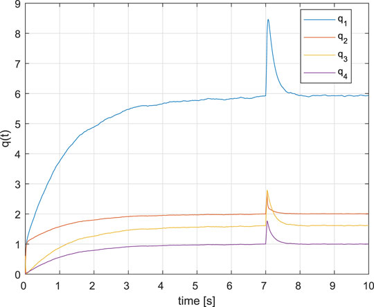
FIGURE 1. The system state variables time response.

FIGURE 2

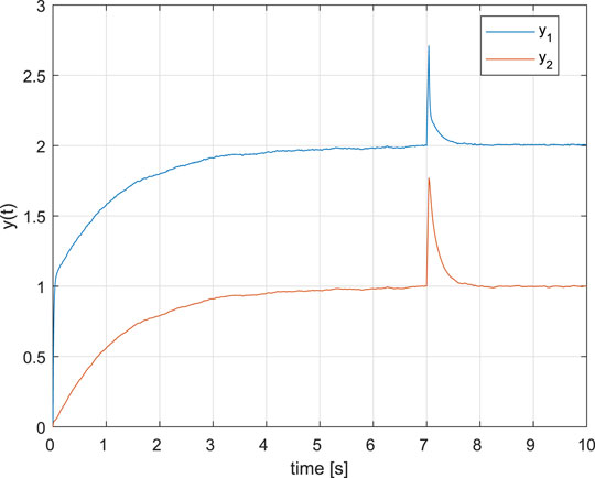
FIGURE 2. The system output variables time response.

Since the dynamics of state observers is projected in the dynamics of observer-based fault residual generators, an algorithm, the discrete version of which is given in Krokavec and Filasová (2012), can be used for detection and localization of actuator faults. To process in the considered task the produced residual signal to an actuator fault detection, the bank of two set of thresholds is applied, where each of them uses one of the actuator fault residual signal model to actuate the decision logic for single actuator fault detection and localization. The result is activation of the VA and the gain matrix M_f, corresponding to the detected fault. Of course, like any fault detection and localization subsystem, this structure also has a finite positive response time.

The main illustrative contribution of this example is the detailed explanation of the VA design steps, based on the system constraint interpretation and a single actuator fault interval limits incorporation in the LMI algorithm, including the implementation algorithm for strictly Metzler continuous-time linear systems.

6 Concluding Remarks

According to the control theory of positive linear continuous-time systems, in the paper is presented one design method which gives desired stability of the faulty system via activation of the linear VA after a single actuator fault occurrence and this method is theoretically substantiated. The main contribution is giving the sets of design conditions for stability of the system in the nominal mode and for stability of faulty system with VAs, guaranteeing positiveness of such solutions.

Outlining specific aspects of construction, the structural flexibility of this multi-constrained problem suggests to treat the FTC design separately, what has a strong practical point of view. Thus, one of the contributions of the presented approach is the separation of the VA synthesis scheme and the static output control design task, respecting the fundamentally different LMI algorithms and preserving the structure of Metzler matrices, when defining the properties of positive continuous-time linear systems.

The major concepts, in the nominal control parameter design and in the VA synthesis, are formulated using the sets of LMIs, to allow the system parameter representation when reflecting the diagonal stabilization principle, strictly limiting the synthesis tasks for positive continuous-time linear systems. The state-feedback principle in VA design guarantees almost-global asymptotic stability of the faulty system after VA activation. The proposed design approaches provide computationally checkable tools, based on representative analysis. The other results (e.g., Shen and Lam (2015); Bhattacharyya and Patra (2018)) had their main limitation in the computability based on linear programming, guaranteeing non-negative parameters in design. The advantage of the proposed method is an equivalently reformulation of this task for strictly Metzler systems in a more explicit form that makes use of strictly LMIs.

The application of the proposed approach requires that a fault detection and isolation subsystem is available. However, it becomes clear that the desired performances depend on the fault isolation time, but a suitable conjunction of the all dynamic components potentially allows good adaptation to the time limit of fault detection.

For future research, generalized algorithms will be studied to incorporate interactions of actuator fault interval representations into design conditions. Metzler-Takagi-Sugeno models will be studied to overcome the problem that the actuator gain loss can take no clear boundaries. It remains also as a future topic to extend the presented results to distributed system fault diagnosis and fault tolerant control. The currently known design techniques do not overcome the obstacles related with uncertain non-Metzler matrices and so suitable similarity transformations the will also be of subject of authors’ future interest to make proposed procedure applicable to a wider class of systems.

Data Availability Statement

The original contributions presented in the study are included in the article/Supplementary Material, further inquiries can be directed to the corresponding author.

Author Contributions

AF elaborated the principles of the nominal closed-loop control law parameter synthesis and implemented their numerical validation, DK addressed the VA design and constraint principle assembling into set of LMIs in design for Metzler continuous-time linear MIMO systems.

Funding

The research covering the work field presented in this paper was founded by VEGA, the Grant Agency of the Ministry of Education and Academy of Science of Slovak Republic, under Grant No. 1/0483/21.

Conflict of Interest

The authors declare that the research was conducted in the absence of any commercial or financial relationships that could be construed as a potential conflict of interest.

Publisher’s Note

All claims expressed in this article are solely those of the authors and do not necessarily represent those of their affiliated organizations, or those of the publisher, the editors, and the reviewers. Any product that may be evaluated in this article, or claim that may be made by its manufacturer, is not guaranteed or endorsed by the publisher.

Acknowledgments

This support is very gratefully acknowledged.

References

Bellman, R. (1970). Introduction to Matrix Analysis. New York: McGraw-Hill.

Google Scholar

Berman, A., and Hershkowitz, D. (1983). Matrix diagonal Stability and its Implications. SIAM. J. Algebraic Discrete Methods 4 (3), 377–382. doi:10.1137/0604038

CrossRef Full Text | Google Scholar

Berman, A., Neumann, M., and Stern, R. (1989). Nonnegative Matrices in Dynamic Systems. New York: John Wiley & Sons.

Google Scholar

Berman, A., and Plemmons, R. J. (1979). Nonnegative Matrices in the Mathematical Sciences. New York: Academic Press.

Google Scholar

Bessa, I., Puig, V., and Palhares, R. M. (2021). Passivation Blocks for Fault Tolerant Control of Nonlinear Systems. Automatica 125, 1–8. doi:10.1016/j.automatica.2020.109450

CrossRef Full Text | Google Scholar

Bhattacharyya, S., and Patra, S. (2018). Static Output-Feedback Stabilization for MIMO LTI Positive Systems Using LMI-Based Iterative Algorithms. IEEE Control. Syst. Lett. 2 (2), 242–247. doi:10.1109/lcsys.2018.2816969

CrossRef Full Text | Google Scholar

Bolajraf, M., Rami, M. A., and Helmke, U. (2011). Robust Positive Interval Observers for Uncertain Positive Systems. IFAC Proc. 44 (1), 14330–14334. doi:10.3182/20110828-6-it-1002.03682

CrossRef Full Text | Google Scholar

Brewer, J. (1978). Kronecker Products and Matrix Calculus in System Theory. IEEE Trans. Circuits Syst. 25 (9), 772–781. doi:10.1109/tcs.1978.1084534

CrossRef Full Text | Google Scholar

Cvetković, A. (2020). Stabilizing the Metzler Matrices with Applications to Dynamical Systems. Calcolo 57. doi:10.1007/s10092-019-0350-3

CrossRef Full Text | Google Scholar

De Leenheer, P., and Aeyels, D. (2001). Stabilization of Positive Linear Systems. Syst. Control. Lett. 44 (4), 259–271. doi:10.1016/s0167-6911(01)00146-3

CrossRef Full Text | Google Scholar

Ding, S. X. (2021). Advanced Methods for Fault Diagnosis and Fault-Tolerant Control. Berlin: Springer.

Google Scholar

Do, M. H., Koenig, D., and Theilliol, D. (2021). Robust Observer‐based Controller for Uncertain‐stochastic Linear Parameter‐varying (LPV) System under Actuator Degradation. Int. J. Robust Nonlinear Control. 31 (2), 662–693. doi:10.1002/rnc.5302

CrossRef Full Text | Google Scholar

Du, D., Xu, S., and Cocquempot, V. (2021). Observer-Based Fault Diagnosis and Fault-Tolerant Control for Switched Systems Singapore. Springer Nature.

Google Scholar

Farina, L., and Rinaldi, S. (2000). Positive Linear Systems. Theory and Applications. New York: John Wiley & Sons.

Google Scholar

Filasová, A., and Krokavec, D. (2012). H∞ Control of Discrete-Time Linear Systems Constrained in State by equality Constraints. Int. J. Appl. Mathematics Computer Sci. 22 (3), 551–560. doi:10.2478/v10006-012-0042-5

CrossRef Full Text | Google Scholar

Gouzé, J. L., Rapaport, A., and Hadj-Sadok, M. Z. (2000). Interval Observers for Uncertain Biological Systems. Ecol. Model. 133 (1), 45–56. doi:10.1016/s0304-3800(00)00279-9

CrossRef Full Text | Google Scholar

Gritli, H., Zemouche, A., and Belghith, S. (2021). On LMI Conditions to Design Robust Static Output Feedback Controller for Continuous-Time Linear Systems Subject to Norm-Bounded Uncertainties. Int. J. Syst. Sci. 52 (1), 12–46. doi:10.1080/00207721.2020.1818145

CrossRef Full Text | Google Scholar

Horn, R. A., and Johnson, C. R. (1995). Matrix Analysis. New York: Cambridge University Press.

Google Scholar

Hu, Q., Li, B., Xiao, B., and Zhang, Y. (2021). Control Allocation for Spacecraft under Actuator Faults Singapore. Springer Nature.

Google Scholar

Huang, S., Tan, K. K., Er, P. V., and Lee, T. H. (2020). Intelligent Fault Diagnosis and Accommodation Control. Boca Raton: CRC Press.

Google Scholar

Krokavec, D., and Filasová, A., (2021a). A Metzler-Lipschitz Structure in Unknown-Input Observer Design, In Proceedings of the 29th Mediterranean Conference on Control and Automation MED 2021, 831–836. doi:10.1109/med51440.2021.9480199

CrossRef Full Text | Google Scholar

Krokavec, D., and Filasová, A., (2020). Control Design for Linear Strictly Metzlerian Descriptor Systems. In Proceedings of the 18th European Control Conference ECC 2020, 2092–2097. doi:10.23919/ecc51009.2020.9143605

CrossRef Full Text | Google Scholar

Krokavec, D., and Filasová, A., (2021b). Control of Discrete-Time State-Multiplicative Systems with Polytopic Region of Uncertainty. In Proceedings of the 23th International Conference Process Control PC 2021, 31–36. doi:10.1109/pc52310.2021.9447505

CrossRef Full Text | Google Scholar

Krokavec, D., and Filasová, A. (2019). H∞ Norm Principle in Residual Filter Design for Discrete-Time Linear Positive Systems. Eur. J. Control. 45, 17–29. doi:10.1016/j.ejcon.2018.10.001

CrossRef Full Text | Google Scholar

Krokavec, D., and Filasová, A. (2018). LMI Based Principles in Strictly Metzlerian Systems Control Design. Math. Probl. Eng. 2018, 1–14. doi:10.1155/2018/9590253

CrossRef Full Text | Google Scholar

Krokavec, D., and Filasová, A. (2012). Novel Fault Detection Criteria Based on Linear Quadratic Control Performances. Int. J. Appl. Mathematics Computer Sci. 22 (4), 929–938. doi:10.2478/v10006-012-0069-7

CrossRef Full Text | Google Scholar

Krokavec, D., Filasová, A., Serbák, V., and Liščinský, P. (2016). “H $$_{\infty }$$ Approach to Virtual Actuators Design,” in Advanced and Intelligent Computations in Diagnosis and Control. Editor Z. Kowalczuk Cham: Springer Nature, 209–222. doi:10.1007/978-3-319-23180-8_15

CrossRef Full Text | Google Scholar

Lan, J., and Patton, R. J. (2021). Robust Integration of Model-Based Fault Estimation and Fault-Tolerant Control. Cham: Springer Natur.

Google Scholar

Mazenc, F., and Bernard, O. (2011). Interval Observers for Linear Time-Invariant Systems with Disturbances. Automatica 47 (1), 140–147. doi:10.1016/j.automatica.2010.10.019

CrossRef Full Text | Google Scholar

Metzler, W. H. (2016). On the Roots of Matrices. Sydney: Wentworth Press.

Google Scholar

Moore, R. E., Kearfott, R. B., and Cloud, M. J. (2009). Introduction to Interval Analysis. Philadelphia: Society for Industrial and Applied Mathematics.

Google Scholar

Nikaido, H. (1968). Convex Structures and Economic Theory. New York: Academic Press.

Google Scholar

Peaucelle, D., Henrion, D., Labit, Y., and Taitz, K. (2002). User’s Guide for SeDuMi Interface 1.04Toulouse. LAAS-CNRS.

Google Scholar

Prempain, E., and Postlethwaite, I. (2007). “Output Feedback H_∞ Loop-Shaping Controller Synthesis,” in Mathematical Methods for Robust and Nonlinear Control. Editors M. C. Turner, and D. G. Bates (Berlin: Springer-Verlag), 175–194.

Google Scholar

Raïssi, T., and Efimov, D. (2018). Some Recent Results on the Design and Implementation of Interval Observers for Uncertain Systems. Automatisierungstechnik 66 (3), 213–224. doi:10.1515/auto-2017-0081

CrossRef Full Text | Google Scholar

Rauh, A., Dehnert, R., Romig, S., Lerch, S., and Tibken, B. (2021). Iterative Solution of Linear Matrix Inequalities for the Combined Control and Observer Design of Systems with Polytopic Parameter Uncertainty and Stochastic Noise. Algorithms 14 (7205), 1–23. doi:10.3390/a14070205

CrossRef Full Text | Google Scholar

Richter, J. H. (2011). Reconfigurable Control of Nonlinear Dynamical Systems. A Fault-Hiding Approach. Berlin: Springer-Verlag. doi:10.1007/978-3-642-17628-9

CrossRef Full Text | Google Scholar

Scherer, C., Gahinet, P., and Chilali, M. (1997). Multiobjective Output-Feedback Control via LMI Optimization. IEEE Trans. Automat. Contr. 42 (7), 896–911. doi:10.1109/9.599969

CrossRef Full Text | Google Scholar

Shen, J. (2017). Analysis and Synthesis of Dynamic Systems with Positive Characteristics(Singapore. Springer Nature).

Google Scholar

Shen, J., and Lam, J. (2015). On Static Output-Feedback Stabilization for Multi-Input Multi-Output Positive Systems. Int. J. Robust. Nonlinear Control. 25 (16), 3154–3162. doi:10.1002/rnc.3256

CrossRef Full Text | Google Scholar

Smith, H. L. (1995). Monotone Dynamical Systems. An Introduction to the Theory of Competitive and Cooperative Systems. Providence: American Mathematical Society). doi:10.1090/surv/041

CrossRef Full Text | Google Scholar

Steffen, T. (2005). Control Reconfiguration of Dynamical Systems. Linear Approaches and Structural Tests. Berlin: Springer-Verlag.

Google Scholar

Tabatabaeipour, S. M., Stoustrup, J., and Bak, T. (2015). Fault-tolerant Control of Discrete-Time LPV Systems Using Virtual Actuators and Sensors. Int. J. Robust Nonlinear Control. 25 (5), 707–734. doi:10.1002/rnc.3194

CrossRef Full Text | Google Scholar

Zhang, M., Shi, P., ShenWu, C. Z. G., and Wu, Z.-G. (2020). Static Output Feedback Control of Switched Nonlinear Systems with Actuator Faults. IEEE Trans. Fuzzy Syst. 28 (8), 1600–1609. doi:10.1109/tfuzz.2019.2917177

CrossRef Full Text | Google Scholar