Control of Jump Markov Uncertain Linear Systems With General Probability Distributions

1 Introduction

For some systems to be controlled, the dynamics can only be represented with inherent uncertainty, stemming not only from disturbance quantities, but also from uncertain operating modes leading to different parameterization or even varying topology. Examples are production lines, in which units may be temporarily unavailable, or cyber-physical systems embedding communication networks, in which link failures lead to reduced transmission rates or varied routing. If the underlying continuous-valued dynamics is linear, jump Markov linear systems (JMLS) are a suitable means for representing the dynamics. In this system class, the transitions between different operating modes with associated linear dynamics are modeled by Markov chains (Costa et al., 2005). If disturbances are present in addition, the dynamics of each mode comprises stochastic variables with appropriate distribution. The control of JMLS has found considerable attention in recent years, e.g. with respect to determining state feedback control laws for infinite and finite quadratic cost functions (Do Val and Basar, 1997; Park et al., 1997).

Many research groups have focused on schemes of model-predictive control (MPC) for JMLS, motivated by the fact that MPC enables one to include constraints (Maciejowski, 2002). Since the states and inputs of almost all real-world systems have to be kept in feasible or safe ranges, this aspect is a crucial one. The first contributions to constrained control of JMLS date back to the work (Costa and Filho, 1996; Costa et al., 1999), in which state feedback control laws have been determined. Additionally, their control designs consider uncertainties in the initial state and in the transition matrix of the Markov chain. An approach for unconstrained JMLS with additive stationary disturbances based on MPC was proposed in (Vargas et al., 2004), embedding a procedure to determine a set of state feedback controllers. In designing such controllers for bounded additive disturbances, formulations using semi-definite program are well-known (Park et al., 2001; Park and Kwon, 2002; Vargas et al., 2005). For constrained JMLS, an MPC scheme was presented in (Cai and Liu, 2007), in which embedded feedback controllers are synthesized based on linear matrix inequalities, too. Subsequent work improved this approach in (Liu, 2009; Lu et al., 2013; Cheng and Liu, 2015) by using dual-mode predictive control policies, periodic control laws, and multi-step state feedback control laws. In (Yin et al., 2013; Yin et al., 2014), MPC approaches have been presented which ensure robust stability in case of uncertain JMLS.

The mentioned MPC approaches for JMLS are all based on the principle of strict satisfaction of the specified constraints. However, in the case of modeling uncertainties in terms of stochastic variables with unbounded supporting domain, the satisfaction of constraints with high confidence only is a reasonable alternative, leading to a form of soft constraints. For such a probabilistic perspective on constraint satisfaction, which is also adopted in this paper, two approaches are used in literature: In the first one, only the expected values of the random variables are constrained in strict form, and then are referred to expectation constraints. In (Vargas et al., 2006), the first and second moments of the state and input have been considered in this form. In (Tonne et al., 2015), only the first moment was strictly constrained, but the computational complexity has been reduced significantly for higher-dimensional JMLS. In the second approach, the constraints are formulated such that the distribution of the stochastic variables has to satisfy the constraints with a high confidence, then termed chance constraints. Some papers following this principle use particle filter control (Blackmore et al., 2007; Blackmore et al., 2010; Farina et al., 2016; Margellos, 2016), in which a finite set of samples is used to approximate the probability distributions of the JMLS. Typically, these approaches are formulated in form of mixed-integer linear programming problems. While these approaches can handle arbitrary distributions, the computational complexity rises exponentially for increasing the dimension of the spaces of the JMLS or for large prediction horizons. Following a different concept, the work in (Chitraganti et al., 2014) transforms the stochastic problem into a deterministic one (Chitraganti et al., 2014), but the method is restricted to Gaussian distributions of the stochastic variables. The same applies to the approach in (Asselborn and Stursberg, 2015; Asselborn and Stursberg, 2016), which uses probabilistic reachable sets to solve optimization problems with chance constraints, and the work does not use a prediction scheme. The authors of (Lu et al., 2019) have proposed a stochastic MPC approach for uncertain JMLS using affine control laws, but this scheme is restricted to bounded distributions.

Apart from the last-mentioned paper, all previous ones are tailored to Gaussian distributions. In contrast, the paper on hand aims at proposing a control approach by which JMLS with general (bounded or unbounded) distributions are transferred into a target set while chance constraints are satisfied and the computational effort is relatively low. The key step is an analytic approximation of the distribution to reformulate the stochastic control problem into a deterministic one. A method for computing bounds for the covariance matrix is proposed, which enables to compute probabilistic reachable sets (PRS) for the underlying dynamics. The determination of PRS for jump Markov systems has already been considered in (LygerosCassandras, 2007; Abate et al., 2008; Kamgarpour et al., 2013), but these approaches cannot handle arbitrary probability distributions. Here, we use a tightened version of these sets in order to achieve the satisfaction of chance constraint for the states. Furthermore, a scheme of stochastic MPC, which builds on over-approximated probabilistic reachable sets (PRS) for the given arbitrary probability distributions, is proposed in order to realize the transfer of the JMLS into a target set for arbitrary sequences of the discrete state. The paper is organized as follows: Section 2 clarifies some notation used throughout the paper, and introduces the considered system class as well as the control problem. Section 3 describes the procedure for designing the control law, the handling of the construction and approximation of the probabilistic constraints, the determination of the prediction equations, and the predictive control. A numerical example for illustration is in Section 4, before Section 5 concludes the paper.

2 Problem Statement

2.1 Notation

Within this paper, weighted 2-norms are written as $\Vert x{\Vert }_Q^2=x^{T}Qx$, and Q > 0 refers to a positive definite matrix. Let ${\mathbb{S}}^n$ be the set of all symmetric matrices of dimension n.

The standard Kronecker product is denoted by ⊗, and the Minkowski difference by ⊖. The operator vec(M) returns a vector which stacks all elements of the matrix M column-wise.

A distribution $v\sim {\mathcal{G}}_v$ is represented by its expected value q_v as well as its covariance matrix Q_v.

An ellipsoidal set ɛ(q, Q) is parametrized by a center point $q\in {\mathbb{R}}^n$, and a symmetric positive shape matrix $Q\in {\mathbb{S}}^n$:

$\epsilon \left(q,Q\right)=\left\{x\in {\mathbb{R}}^n|{\left(x-q\right)}^T{Q}^{-1}\left(x-q\right)\le 1\right\}.$

If an ellipsoidal set is transformed by an affine function f(x) = Mx + b with $M\in {\mathbb{R}}^{n\times n}$ and $b\in {\mathbb{R}}^n$, the result is again an ellipsoidal set:

$M\cdot \epsilon \left(q,Q\right)+b=\epsilon \left(Mq+b,MQ{M}^T\right).$

2.2 The Control Task

Consider the following type of jump Markov linear and time-invariant system (JMLS) with continuous state $x_k\in {\mathbb{R}}^n$, continuous input $u_k\in {\mathbb{R}}^m$, and disturbance $w_k\in {\mathbb{R}}^n$:

$\begin{array}{ll}\hfill x_{k+1}=& A_{{\theta }_k}{x}_k+B_{{\theta }_k}{u}_k+G_{{\theta }_k}{w}_k,\hfill \\ \hfill \mathcal{M}=& \left(\mathrm{\Theta },P_{\mathcal{M}},{\mu }_0\right),\hfill \\ \hfill x_0& \sim {\mathcal{G}}_x,w_k\sim {\mathcal{G}}_w.\hfill \end{array}(1)$

In here, the initial continuous state x₀ as well as the disturbance w_k as stochastic variables are selected from arbitrarily selected distributions ${\mathcal{G}}_x$ and ${\mathcal{G}}_w$. The expected values q₀ and q_w of these variables as well as covariance matrices Q₀ and Q_w are assumed, however, to be known. Let θ_k ∈ Θ denote a discrete state of the Markov chain $\mathcal{M}$, and θ_k selects the system matrices from the sets A = {A_i | i ∈ Θ}, B = {B_i | i ∈ Θ}, and G = {G_i | i ∈ Θ}. The probability distribution of θ_k is denoted by μ_k with μ_i,k =  Pr(θ_k = i). The conditional transition probabilities are defined as p_i,m≔  Pr(θ_k+1 = i | θ_k = m) for i, m ∈ Θ, and by collecting all of these probabilities, the transition matrix $P_{\mathcal{M}}={[p_{i,m}]}_{i,m\in \mathrm{\Theta }}$ is formed.

Assumption 1. The system state x_k, the Markov state θ_k, as well as the probability distribution μ_k are measurable. Furthermore, the distributions of x₀ and w_k are independent.

The measurability assumption of the Markov state and its probability distribution is quite common for JMLS. If the Markov state is used to model whether a process is in a nominal or a failure state, and if a suitable failure detection mechanism exists for the process, this assumption is certainly justified. Note that only the Markov state in the current time step k is assumed to be measurable, while the next transitions is unknown. For a system of type (1), let a terminal set $\mathcal{T}\subset \mathcal{X}$ with $0\in \mathcal{T}$ and an initial state x₀ be given, where the latter is sampled from the distribution ${\mathcal{G}}_x$.

Furthermore, let admissible state and input sets be defined by:

$\mathcal{X}=\left\{x\in {\mathbb{R}}^n|R_{x}x\le b_x\right\},(2)$

$\mathcal{U}=\left\{u\in {\mathbb{R}}^m|R_{u}u\le b_u\right\}(3)$

as polytopes, which are parameterized by $R_x\in {\mathbb{R}}^{n_x\times n}$, $b_x\in {\mathbb{R}}^{n_x}$ and $R_u\in {\mathbb{R}}^{n_u\times m}$, $b_u\in {\mathbb{R}}^{n_u}$ respectively.

Then, the control problem investigated in this paper is to find a control strategy ϕ_u = {u₀, u₁, …, u_N−1}, $N\in \mathbb{N}$ leading to a continuous state sequence ϕ_x = {x₀, x₁, …, x_N} which satisfies, irrespective of the uncertain discrete state sequence ϕ_θ = {θ₀, θ₁, …, θ_N}, that:

• ϕ_u stabilizes the JMLS with confidence δ,

• ϕ_x and ϕ_u fulfill the chance constraints:

$\mathit{Pr}\left(x_k\in \mathcal{X}\right)\ge {\delta }_x,(4)$

$\mathit{Pr}\left(u_k\in \mathcal{U}\right)\ge {\delta }_u(5)$

in any time step k and for any disturbances w_k,

• and for which a finite $N\in \mathbb{N}$ exists such that $\mathit{Pr}(x_N\in \mathcal{T})\ge {\delta }_x$.

3 Probabilistic Control of Jump Markov Affine Systems

In order to solve the stated control problem, this paper proposes a new method which combines concepts of stochastic model predictive control (SMPC), the conservative approximation of the distributions ${\mathcal{G}}_x$ and ${\mathcal{G}}_w$ and the computation of stochastic reachable set of the JMLS. The approach also includes a scheme to modify the chance constraints tailored to the approximated distribution, and the use of embedded feedback controllers to take care of the disturbances and to shape the state distribution along the system evolution.

An underlying principle is to separate the evolution of the continuous state into a part referring to the expected state and a part encoding the deviation from the latter, as also followed in some approaches of tube-based MPC (Fleming et al., 2015). This principle allows for a control strategy, in which the expected state is steered towards the target set by a solving a deterministic optimization problem within the MPC part, as was proposed in (Tonne et al., 2015). The fact that repeated optimization on rolling horizons is used rather than the offline solution of one open-loop optimal control problem not only tailors the scheme to online solution, but also reduces the computational effort due to the possibility of employing rather short horizons. For the deviation part of the dynamics, a new scheme based on probabilistic reachable sets is established, which are computed and used for constraint tightening of the MPC formulation to satisfy the chance constraints (Eqs 4, 5). Since these sets depend on the covariances of the continuous system states and thus, on future discrete states of the JMLS, a boundary of the covariances for arbitrary sequences of the Markov state can be established. One of the main contributions of this paper is that a control strategy is derived which stabilizes the uncertain JMLS into the target with a specified and high probability.

3.1 Structure of the Control Strategy

To design a control strategy for the given problem, the probabilistic continuous system state x_k as well as the disturbance w_k are split into an expected and an error part:

$x_k=q_k+e_k,q_k≔\mathbb{E}\left[x_k\right],(6)$

$w_k=q_w+e_{w,k},q_w≔\mathbb{E}\left[w_k\right].(7)$

Similar to methods of MPC employing reachability tubes, see e.g., (Fleming et al., 2015), a local affine control law of the form

$u_k=v_k-K_i\left(x_k-q_k\right),(8)$

is defined, in which v_k is the expected value of u_k. The state feedback matrix K_i is determined off-line, such that A_cl,i = A_i − B_iK_i for i ∈ Θ is stable. Note that stability here refers only to A_cl,i, not to that the complete switching dynamics. The stability of the JMLS will be taken care of later in this section. The feedback matrix K_i of the control law ensures that the error part e_k is kept in a neighborhood of q_k. By applying the control law (8) to the dynamics (1), the following difference equations for the expected value q_k and error e_k of x_k are obtained:

$q_{k+1}=A_{{\theta }_k}{q}_k+B_{{\theta }_k}{v}_k+G_{{\theta }_k}{q}_w,(9)$

$e_{k+1}=\underset{=A_{cl,{\theta }_k}}{\underbrace{\left(A_{{\theta }_k}-B_{{\theta }_k}{K}_{\theta }\right)}}{e}_k+G_{{\theta }_k}{e}_{w,k}.(10)$

The stochastic term e_w,k of the uncertainty is considered in Eq. 10, while Eq. 9 considers only the deterministic part (expected value) q_w. Since the error part encodes the covariance of x_k around the expected value q_k, the following difference equation for the covariance matrix Q_k results from using linear transformation of the covariance matrices:

$Q_{k+1}=A_{cl,{\theta }_k}{Q}_k{A}_{cl,{\theta }_k}^T+G_{{\theta }_k}{Q}_w{G}_{{\theta }_k}^T.(11)$

As already mentioned, an approach of SMPC is chosen in the upcoming parts of the paper to determine a sequence of expected inputs v_k+j|k, such that the expected value of x_k will be transferred and stabilized into the target set. SMPC has the crucial advantage (compared to optimal control), that the sequence of input signals are computed on-line based on the current discrete state which can be measured, see Asm. 1. Thus, the probabilistic reachable sets can be computed with higher accuracy. Since Eq. 9 is only stochastic with respect to the Markov state θ_k, the SMPC scheme can be formulated as a deterministic predictive control scheme with respect to the expected values of x_k. This scheme predicts the future expected continuous states over a finite horizon using the affine dynamics Eq. 9. To ensure that a certain share of all possible x_k (according to the underlying distributions) satisfies the constraints, the feasible set of states and inputs is reduced. This step of constraint tightening is described in detail in Section 3.4.

3.2 Construction of PRS Using the Chebyshev Inequality

In order to satisfy the chance constraints (4) and (5), probabilistic reachable sets for the error part of the continuous states are computed and used for tightening the original constraints. This allows one to use the reformulated constraints in a deterministic version of an optimization problem (with the MPC scheme) with respect to the continuous state of the JMLS. Probabilistic reachable sets are first defined as follows:

Def. 1. A stochastic reachable set contains all error parts which are reachable according to Eq. 10 from an initial set ${\mathcal{R}}_0$ with a probability of at least δ_x, given the disturbances $w_k\sim {\mathcal{G}}_w$:

$e_0\in {\mathcal{R}}_0\Rightarrow \mathit{Pr}\left(e_k\in {\mathcal{R}}_k\right)\ge {\delta }_x,k\in \left\{\mathrm{0,1},\dots ,N\right\}.$

In the general case, the computation of the true PRS may turn out to be difficult and can result in non-convex sets. If so, the true PRS can be be over-approximated by convex sets as described in the following: as a main contribution of this paper, it is proposed to use the Chebychev inequality (Marshall and Olkin, 1960) to conservatively bound the true PRS. The n-dimensional Chebyshev inequality for random variables provides a lower bound on the probability that an ellipsoidal set contains a realization of the stochastic variable. Thus, the inequality can be used to approximate the true reachable sets by ellipsoids in case that the expected value as well as the covariance matrix of the random variable is known.

Theorem 3.1. Let X be a random variable with finite expected value $q=\mathbb{E}[X]$ and covariance matrix Q = Cov(X) > 0. Then

$\mathit{Pr}\left({\left(X-q\right)}^T{Q}^{-1}\left(X-q\right)\le \delta \right)\ge 1-\frac{n}{\delta },$

for all δ > 0.

PROOF. (Ogasawara, 2019). Consider the transformed new random variable Z:

$Z={\left(X-q\right)}^T{Q}^{-1}\left(X-q\right).$

Since Q > 0, the random variable Z can be decomposed as follows:

$Z=Y^{T}Y,\text{where}Y=Q^{-\frac{1}{2}}\left(X-q\right)$

The random variable Y satisfies

$\mathbb{E}\left[Y\right]=\mathbb{E}\left[Q^{-\frac{1}{2}}\left(X-q\right)\right]=Q^{-\frac{1}{2}}\left(\mathbb{E}\left[X\right]-q\right)=0,$

and

$\text{Cov}\left(Y\right)=\text{Cov}\left(Q^{-\frac{1}{2}}\left(X-q\right)\right)=Q^{-\frac{1}{2}}\text{Cov}\left(X\right)Q^{-\frac{1}{2}}=I.$

Therefore,

$\mathbb{E}\left[Z\right]=\mathbb{E}\left[Y^{T}Y\right]=\mathbb{E}\left[\sum _{i=1}^n{Y}_i^2\right]=\sum _{i=1}^n\mathbb{E}\left[Y_i^2\right]=\sum _{i=1}^n\text{Var}\left(Y_i\right)=n.$

Finally, by using the Markov’s inequality,

$\mathit{Pr}\left({\left(X-q\right)}^T{Q}^{-1}\left(X-q\right)\le \delta \right)=\mathit{Pr}\left(Z\le \delta \right)\ge 1-\frac{\mathbb{E}\left[Z\right]}{\delta }=1-\frac{n}{\delta }$

holds for all δ > 0.

Now, the Chebyshev inequality is used to formulate a bound on the probability that the error part of the continuous state x_k of the JMLS at time k is contained in an ellipsoid around the origin:

$\mathit{Pr}\left(\underset{=e_k\in \epsilon \left(0,Q_k^{\delta }\right)}{\underbrace{e_k^T{Q}_k^{-1}{e}_k\le \delta }}\right)\ge \underset{={\delta }_x}{\underbrace{1-\frac{n}{\delta }}}.(12)$

In here, the matrix $Q_k^{\delta }=n/(1-{\delta }_x)\cdot Q_k$ is a scaled shape matrix of the over-approximating ellipsoid which contains the realizations of e_k at least with probability δ_x. While this approximation may introduce conservatism, the important point is that this inequality applies to arbitrary distributions. For computation of the ellipsoidal sets, the ellipsoidal calculus can be used, see (Kurzhanskii and Vàlyi, 1997). With $Q_k^{\delta }$, the over-approximating PRS can now be expressed by:

${\mathcal{R}}_k=\epsilon \left(0,Q_k^{\delta }\right).$

Nevertheless, this leads to time-varying constraints which depend on the discrete state of the JMLS. To reduce the computational complexity, and thus the computation time, a possible alternative is to use a more conservative approximation of the constraints, such that they remain time-invariant and independent of θ_k, as described in the following.

3.3 Bounding the State Covariance Matrix

For time-invariant constraints being independent of the discrete state of the JMLS, the shape matrices $Q_k^{\delta }$, k ∈ {1, …, N} can be over-approximated by a static matrix $Q_{\infty }^{\delta }$, such that:

${\mathcal{R}}_k\epsilon \left(0,Q_k^{\delta }\right)\subseteq \epsilon \left(0,Q_{\infty }^{\delta }\right)=:{\mathcal{R}}_{\infty },\forall k\in \left\{1,\dots ,N\right\}(13)$

holds for all states θ_k ∈ Θ. Note that $Q_{\infty }^{\delta }$ is equal to the solution of a Lyapunov equation, if there is only one mode. Before detailing the method, the following definitions are required:

Def. 2. For any symmetric matrix $S\in {\mathbb{S}}^n$, let an operator svec be defined as:

$\begin{array}{ll}\hfill \text{svec}\left(S\right)≔& \left[s_{11},\sqrt{2}{s}_{21}\dots ,\sqrt{2}{s}_{n1},s_{22},\sqrt{2}{s}_{32},\dots ,\right.\hfill \\ \hfill & {\left.\dots ,\sqrt{2}{s}_{n2},\dots ,s_{nn}\right]}^T.\hfill \end{array}$

i.e., the elements of S are stacked columnwise, and the off-diagonal elements are multiplied by $\sqrt{2}$.

Def. 3. The symmetric Kronecker product of two matrices $D,M\in {\mathbb{R}}^{n\times n}$ is defined by:

$D{\otimes }_{s}M≔T\left(D\otimes M\right)T^T,$

where $T\in {\mathbb{R}}^{\frac{n}{2}(n+1)\times n}$ is an orthogonal matrix with:

$T\cdot \text{vec}\left(S\right)=\text{svec}\left(S\right),T^T\cdot \text{svec}\left(S\right)=\text{vec}\left(S\right).$

By using the definitions above, the covariance difference Eq. 11 turns into a pseudo-affine system:

$\text{svec}\left(Q_{k+1}\right)=\underset{=:{\mathrm{\Phi }}_i}{\underbrace{\left(A_{cl,i}{\otimes }_s{A}_{cl,i}\right)}}\cdot \underset{=:{\phi }_k}{\underbrace{\text{svec}\left(Q_k\right)}}+\underset{=:{\phi }_{w,i}}{\underbrace{\text{svec}\left(G_i{Q}_w{G}_i^T\right)}},(14)$

where φ_k is the pseudo state, and again i ∈ Θ. Note that the next state φ_k+1 = svec(Q_k+1) depends also on the Markov state. Furthermore, let ${\bar{\phi }}_i$ be the steady state of system (14). It can be shown that if A_cl,i is stable, then Φ_i is also stable.

Now a quadratic Lyapunov function $\tilde{V}(\phi )$ is introduced, which is centered in φ_c and which is parametrized by a shape matrix $\tilde{P}={\tilde{P}}^T>0$:

$\tilde{V}\left(\phi \right)={\left(\phi -{\phi }_c\right)}^T\tilde{P}\left(\phi -{\phi }_c\right).$

The center point φ_c of the Lyapunov function is chosen as the mean value of the steady states for the different Markov states. Next, the smallest common invariant set is determined for the pseudo system (14). The common Lyapunov stability condition is given by $\tilde{V}({\phi }_k)-\tilde{V}({\phi }_{k+1})\ge 0$. However, since the JMLS may transition between the Markov states and every i ∈ Θ leads to a different steady state, it cannot always be guaranteed that the value of $\tilde{V}(\phi )$ decreases. In case a descent is locally not possible, the absolute value of $\tilde{V}(\phi )$ is bounded by the following relaxed condition:

$\text{If}\tilde{V}\left({\phi }_{k+1}\right)-\tilde{V}\left({\phi }_k\right)\ge 0,\text{then}\tilde{V}\left({\phi }_{k+1}\right)\le 1.(15)$

By applying the S-procedure to Eq. 15, a corresponding LMI can be obtained for λ > 0:

$\left[\begin{array}{cc}\hfill \left(1+\mathrm{\lambda }\right){\mathrm{\Phi }}_i^T\tilde{P}{\mathrm{\Phi }}_i-\mathrm{\lambda }\tilde{P}\hfill & \hfill \left(1+\mathrm{\lambda }\right){\left({\phi }_{w,i}-{\phi }_c\right)}^T\tilde{P}{\mathrm{\Phi }}_i\hfill \\ \hfill \left(1+\mathrm{\lambda }\right){\mathrm{\Phi }}_i^T\tilde{P}\left({\phi }_{w,i}-{\phi }_c\right)\hfill & \hfill \left(1+\mathrm{\lambda }\right){\left({\phi }_{w,i}-{\phi }_c\right)}^T\tilde{P}\left({\phi }_{w,i}-{\phi }_c\right)-1\hfill \end{array}\right]\le 0.(16)$

The minimum positive definite matrix $\tilde{P}$ is determined such that the set with $\tilde{V}(\phi )\le 1$ contains all steady states of Eq. 14:

$\underset{\tilde{P}}{\min }\text{trace}\left(\tilde{P}\right)(17)$

$\text{s.t.:}(16),{\bar{\phi }}_i\in \epsilon \left({\phi }_c,\tilde{P}\right)\forall i\in \mathrm{\Theta },(18)$

where ${\bar{\phi }}_i$ is the steady state of Eq. 14. If there exists a positive definite matrix $\tilde{P}$ which satisfies (18), then the set ${(\phi -{\phi }_c)}^T\tilde{P}(\phi -{\phi }_c)\le 1$ is an invariant set for the sequence of covariance matrices $Q_k^{\delta }$, k ∈ {1, …, N}. By back-transformation of the solution $\tilde{P}$ and by applying the inverse Kronecker product operator, an upper bound $Q_{\infty }^{\delta }$ of the covariance matrix $Q_k^{\delta }$ for arbitrary sequences of discrete states of the JMLS can be determined.

Theorem 3.2. Let the optimization problem (17)-(18) have a feasible solution. The back transformation of the solution is an over-approximation of all covariance matrices, i.e.

$\underset{k\to \infty }{\lim }\epsilon \left(0,Q_k^{\delta }\right)\subseteq \epsilon \left(0,Q_{\infty }^{\delta }\right)\forall {\theta }_k\in \mathrm{\Theta }.(19)$

PROOF. (Sketch) The transformation of Eqs 11–14 by using Kronecker algebra does not modify the solution for a specific i ∈ Θ (Schäcke, 2004). Consider now arbitrary sequences of i, the set $\mathrm{\Omega }≔\{\phi |\tilde{V}(\phi )\le 1\}$ is invariant as long as the implication Eq. 15 holds, what is ensured by the matrix inequality Eq. 16. When applying back-transformation to the solution, the resulting covariance matrix is an upper bound of $Q_k^{\delta }$, since the back-transformation does again not modify the solution (as the forward transformation).

Note that solving the optimization problem Eqs 17, 18 and thus, the computation of the PRS for the error part e_k of the state x_k can be computationally demanding for larger-scale Markov systems. But this optimization problem has to be solved only once and is carried out offline before starting the online optimization (to be described in the following). The offline computation is possible, since ${\mathcal{R}}_{\infty }=\epsilon (0,Q_{\infty }^{\delta })$ is valid independently of a particular mode and time. In the next subsection, the upper bound $Q_{\infty }^{\delta }$ is used to compute substitute constraints for the optimization in the MPC scheme.

3.4 Computation of the Tightening Constraints and MPC Formulation

In this section, a method to compute the tightened constraints in a stochastic manner for arbitrary distributions is presented. Tightening the constraints plays a crucial role if the optimization problem refers to the (conditional) expected values of x_k [and thus u_k according to the control law (Eq, 8)], as in this paper. Since the true values lie around the expected values (depending on the chosen distribution), the original constraints have to be tightened to ensure satisfaction of the chance constraints Eqs 4, 5. Since the tightening is obtained as the Minkowski difference of $\mathcal{X}$ (or $\mathcal{U}$ respectively) and the PRS, the computation of the PRS is necessary. The tightened constraints are obtained by:

$\mathcal{Q}=\mathcal{X}\ominus {\mathcal{R}}_{\infty }=\mathcal{X}\ominus \epsilon \left(0,Q_{\infty }^{\delta }\right),(20)$

$\mathcal{V}=\mathcal{U}\ominus K_i{\mathcal{R}}_{\infty }=\mathcal{U}\ominus \epsilon \left(0,K_i{Q}_k^{\delta }{K}_i^T\right).(21)$

Note that these computations can be carried out offline. Based on the ellipsoidal form of ${\mathcal{R}}_{\infty }$, the chance constraints Eqs 4, 5 can be reformulated into (linear) hard constraints using (Boyd and Vandenberghe, 2009):

$\underset{=:q_k\in \mathcal{Q}}{\underbrace{r_{x,i}\cdot q_k+\Vert Q_{\infty }^{{\delta }^{\frac{1}{2}}}\cdot r_{x,i}{\Vert }_2\le b_{x,i},\forall i\in \left\{1,\dots ,n_x\right\}}},(22)$

where r_x,i the i-th row of R_x, and b_x,i the i-th entry of b_x, defining the polytope $\mathcal{X}$. The relation (22) can be understood as the condition $q_k\in \mathcal{Q}$. The linearity of the inequality constraints Eq. 22 is guaranteed since the reachable sets of the error part e_k are over-approximated by an ellipsoid with a constant shape matrix $Q_{\infty }^{\delta }$.

The computation of the input constraint (5) follows analogously by determination of an over-approximated matrix for $K_i{Q}_k^{\delta }{K}_i^T$. Let $v_k\in \mathcal{V}$ denote the resulting hard constraint for the input v_k.

The following assumption is necessary for ensuring the existence of a feasible solution of the following optimization problem to be carried out online within the MPC scheme.

Assumption 2. After constraint tightening, the resulting sets $\mathcal{Q}$ and $\mathcal{V}$ are non-empty and contain the origin in their interior. In addition, $\mathcal{Q}$ contains the initial expected value q₀.

Note that if the computations according to Eqs 20, 21 lead to empty sets $\mathcal{Q}$ or $\mathcal{V}$, thus contradicting this assumption, the reduction of δ_x may heal this situation. The optimization problem to be solved in any step of the MPC scheme can finally be expressed as follows:

$\underset{{\varphi }_v}{\min }\Vert q_{k+H|k}{\Vert }_P^2+\sum _{j=0}^{H-1}\Vert q_{k+j|k}{\Vert }_Q^2+\Vert v_{k+j|k}{\Vert }_R^2(23)$

$\text{s.t.\hspace{0.17em}for\hspace{0.17em}all\hspace{0.17em}}j\in \left\{\mathrm{0,1},\dots ,H-1\right\}:(24)$

$q_{k+j+1|k}=A_{{\theta }_{k+j|k}}{q}_{k+j|k}+B_{{\theta }_{k+j|k}}{v}_{k+j|k}+G_{{\theta }_{k+j|k}}{q}_w,(25)$

$q_{k+j|k}\in \mathcal{Q},(26)$

$v_{k+j|k}\in \mathcal{V},(27)$

$q_{k+H|k}\in \mathcal{S}\cdot {\alpha }^{k+H|k},(28)$

with the sequence of expected continuous inputs ϕ_v = {v_k|k, …, v_k+H−1|k} and for a quadratic cost function with matrices P, Q, R > 0. Convergence is enforced by a shrinking ellipsoid $\mathcal{S}≔\{x\in {\mathbb{R}}^n|x^{T}x\le q_0^2\}$ with $\alpha \in \left]\mathrm{0,1}\right[$.

Note that throughout the derivation of this problem, no specific assumptions for the distributions of x₀ and w_k were required. Previous contributions in this field consider bounded distributions or assume that there are normally distributed.

Generally, the constraints Eq. 25 have to be fulfilled for every possible discrete state since the future states are not deterministically known. For JMLS with high-dimensional continuous spaces or many discrete states, as well as instances of the MPC problem with large horizons H, the computational complexity of solving Eq. 23 can be significant. To improve the solution performance, the following section proposes the modification of not only predicting the expected values of x_k and u_k, but also those of the discrete states.

3.5 Prediction Equations for the Expected Discrete State

The solution of the optimization problem Eqs 23–28 requires to determine the predictions q_k+j|k. The recursive procedure proposed in (Tonne et al., 2015) can be used also for Eqs 23–28 in order to determine the predictions with relatively computational effort.

Let the conditional expected value of x_k+j|k under the condition of a discrete predecessor state i be defined as:

${\bar{q}}_{i,k+j|k}≔\mathbb{E}\left[x_{k+j|k}|{\theta }_{k+j-1}=i\right].(29)$

The predicted conditional expected value of the continuous state over all discrete states can then be expressed as:

${\bar{q}}_{k+j|k}=\sum _{i=1}^{|\mathrm{\Theta }|}{\bar{q}}_{i,k+j|k}.(30)$

Due to the Markov property of $\mathcal{M}$, the probability distribution μ can be predicted to ${\mu }_{k+j|k}=P_{\mathcal{M}}^j\cdot {\mu }_k$. In order to formulate the prediction equations depending on q_k, v_k+l|l and q_w, the recursive matrices ${\tilde{A}}_{k+j|k}$, ${\tilde{B}}_{k+j|k}$, and ${\tilde{G}}_{k+j|k}$ can be defined according to (Tonne et al., 2015):

$\begin{array}{ll}\hfill {\tilde{A}}_{i,k+j+1|k}& =A_i\sum _{m=1}^{|\mathrm{\Theta }|}{p}_{i,m}{\tilde{A}}_{m,k+j|k},{\tilde{A}}_{i,k+1|k}={\mu }_{i,k}{A}_i,\hfill \\ \hfill {\tilde{B}}_{i,k+j+1|k}^{\left(l\right)}& =A_i\sum _{m=1}^{|\mathrm{\Theta }|}{p}_{i,m}{\tilde{B}}_{m,k+j|k}^{\left(l\right)},{\tilde{B}}_{i,k+1|k}^{\left(j-1\right)}={\mu }_{i,k+j-1|k}{B}_i,\hfill \\ \hfill {\tilde{G}}_{i,k+j+1|k}^{\left(l\right)}& =A_i\sum _{m=1}^{|\mathrm{\Theta }|}{p}_{i,m}{\tilde{G}}_{m,k+j|k}^{\left(l\right)},{\tilde{G}}_{i,k+1|k}^{\left(j-1\right)}={\mu }_{i,k+j-1|k}{G}_i.\hfill \end{array}$

With these matrices, the prediction Eq. 29 is rewritten to:

${\bar{q}}_{i,k+j|k}={\tilde{A}}_{i,k+j|k}{q}_k+\sum _{l=0}^{j-1}\left({\tilde{B}}_{i,k+j|k}^{\left(l\right)}{v}_{k+l|k}+{\tilde{G}}_{i,k+j|k}^{\left(l\right)}{q}_w\right).$

Using Eq. 30, the conditional expected value ${\bar{q}}_{k+j|k}$ results in:

${\bar{q}}_{k+j|k}=\sum _{i=1}^{|\mathrm{\Theta }|}\left({\tilde{A}}_{i,k+j|k}{q}_k+\sum _{l=0}^{j-1}\left({\tilde{B}}_{i,k+j|k}^{\left(l\right)}{v}_{k+l|k}+{\tilde{G}}_{i,k+j|k}^{\left(l\right)}{q}_w.\right)\right)(31)$

leading to the following form of the optimization problem Eqs 23–28:

$\underset{{\varphi }_v}{\min }\Vert {\bar{q}}_{k+H|k}{\Vert }_P^2+\sum _{j=0}^{H-1}\Vert {\bar{q}}_{k+j|k}{\Vert }_Q^2+\Vert v_{k+j|k}{\Vert }_R^2(32)$

$\text{s.t.}:(31),(33)$

${\bar{q}}_{k+j|k}\in \mathcal{Q},(34)$

$v_{k+j|k}\in \mathcal{V},(35)$

$q_{k+H|k}\in \mathcal{S}\cdot {\alpha }^{k+H|k}.(36)$

Since the Markov state θ_k is measurable, the prediction ${\bar{q}}_{k+1}$ for the first step is deterministic. Thus, the constraints for the first prediction are considered to be satisfied strictly (while the subsequent prediction steps consider the constraints in stochastic form). Due to the repeated optimization in each time step k, these constraints are satisfied in every time instant k, i.e. q_k will be kept within the state constraints if the problem has a solution in each time step.

Theorem 3.3. For the optimization problem Eqs 32–36, consider the case that a feasible solution exists in every time step k. In addition, assume that Q, R, P > 0 and that the problem Eqs 17, 18 has a feasible solution as well. The state of the closed-loop system then converges to the origin with at least a probability of δ_x, i.e.:

$\mathit{Pr}\left(\underset{k\to \infty }{\lim }{x}_k=0\right)\ge {\delta }_x,(37)$

and $\mathit{Pr}({\lim }_{k\to \infty }{x}_k\in \mathcal{T})\ge {\delta }_x$.

PROOF. From Theorem 3.1, the resulting over-approximated sets contain the error parts e_k of x_k with at least a probability of δ_x, independently of the chosen probability distribution, i.e., $\mathit{Pr}(e_k\in \epsilon (0,Q_k^{\delta }))\ge {\delta }_x$. Furthermore, from it follows from Theorem 3.2 that the probabilistic reachable sets of the error e_k are independent of the discrete state and of time:

$\mathit{Pr}\left(e_k\in \epsilon \left(0,Q_{\infty }^{\delta }\right)\right)\ge \mathit{Pr}\left(e_k\in \epsilon \left(0,Q_k^{\delta }\right)\right)\ge {\delta }_x.(38)$

When using constraint tightening based on $\epsilon (0,Q_{\infty }^{\delta })$ and under the Assumption 2, it is sufficient to consider the expected value of x_k: By the last constraint (36), the convergence of the expected value is enforced with increasing k, i.e.

$\underset{k\to \infty }{\lim }{q}_k=0.(39)$

In addition, since the discrete state is measurable (Assumption 1), the constraints of the prediction are always strictly enforced. Finally, by combining (38) and (39), it follows that Pr( lim_k→∞x_k = 0) ≥ δ_x, implying also $\mathit{Pr}({\lim }_{k\to \infty }{x}_k\in \mathcal{T})\ge {\delta }_x$ due to $0\in \mathcal{T}$. □

4 Numerical Example

In order to illustrate the principle of the proposed method, numerical examples are provided in this section. First consider the following small system with n = 2 and |Θ| = 4:

$A_1=\left[\begin{array}{cc}\hfill 1\hfill & \hfill 0.1\hfill \\ \hfill -0.2\hfill & \hfill 0.9\hfill \end{array}\right],B_1=\left[\begin{array}{cc}\hfill -1\hfill & \hfill 0\hfill \\ \hfill 0.5\hfill & \hfill 1\hfill \end{array}\right],G_1=\left[\begin{array}{cc}\hfill 1.3\hfill & \hfill 0\hfill \\ \hfill 0\hfill & \hfill 1\hfill \end{array}\right],$

$A_2=\left[\begin{array}{cc}\hfill -0.9\hfill & \hfill -0.1\hfill \\ \hfill 0\hfill & \hfill 1.1\hfill \end{array}\right],B_2=\left[\begin{array}{cc}\hfill 1\hfill & \hfill 0.5\hfill \\ \hfill 0\hfill & \hfill 2\hfill \end{array}\right],G_2=\left[\begin{array}{cc}\hfill 0.7\hfill & \hfill -0.4\hfill \\ \hfill 0\hfill & \hfill 1.1\hfill \end{array}\right],$

$A_3=\left[\begin{array}{cc}\hfill 0.8\hfill & \hfill 0\hfill \\ \hfill 0.05\hfill & \hfill 0.9\hfill \end{array}\right],B_3=\left[\begin{array}{cc}\hfill 0.5\hfill & \hfill 0.2\hfill \\ \hfill 0\hfill & \hfill 1\hfill \end{array}\right],G_3=\left[\begin{array}{cc}\hfill 0.8\hfill & \hfill 0\hfill \\ \hfill 0\hfill & \hfill 0.7\hfill \end{array}\right],$

$A_4=\left[\begin{array}{cc}\hfill 0.8\hfill & \hfill 0\hfill \\ \hfill -0.2\hfill & \hfill 0.9\hfill \end{array}\right],B_4=\left[\begin{array}{cc}\hfill -1\hfill & \hfill 1\hfill \\ \hfill 0.5\hfill & \hfill 0.8\hfill \end{array}\right],G_4=\left[\begin{array}{cc}\hfill 0.8\hfill & \hfill -0.2\hfill \\ \hfill 0.5\hfill & \hfill 0.3\hfill \end{array}\right].$

The state region (2) is parameterized by:

$\begin{array}{l}\hfill R_x={\left[\begin{array}{ccccccccc}\hfill -4\hfill & \hfill -1\hfill & \hfill -2\hfill & \hfill 0\hfill & \hfill 1\hfill & \hfill -5\hfill & \hfill 4\hfill & \hfill 0\hfill & \hfill 2\hfill \\ \hfill -1\hfill & \hfill 0\hfill & \hfill -1\hfill & \hfill 1\hfill & \hfill 0\hfill & \hfill -1\hfill & \hfill 1\hfill & \hfill -1\hfill & \hfill -1\hfill \end{array}\right]}^T,\\ \hfill b_x={\left[\begin{array}{ccccccccc}\hfill 15\hfill & \hfill 11.5\hfill & \hfill 10\hfill & \hfill 60\hfill & \hfill 3\hfill & \hfill 25\hfill & \hfill 48\hfill & \hfill 7\hfill & \hfill 10\hfill \end{array}\right]}^T,\end{array}$

the input constraints chosen to:

$-3\le u_i\le 3,i\in \left\{\mathrm{1,2}\right\}$

and the chance constraints selected as:

$\mathit{Pr}\left(x_k\in \mathcal{X}\right)=\mathit{Pr}\left(u_k\in \mathcal{U}\right)=0.85.$

The initial distribution of the Markov state is specified by:

${\mu }_0=\left[\begin{array}{cccc}\hfill 1\hfill & \hfill 0\hfill & \hfill 0\hfill & \hfill 0\hfill \end{array}\right],$

and the transition matrix $P_{\mathcal{M}}$ by:

$P_{\mathcal{M}}=\left[\begin{array}{cccc}\hfill 0.25\hfill & \hfill 0.25\hfill & \hfill 0.25\hfill & \hfill 0.25\hfill \\ \hfill 0.25\hfill & \hfill 0.25\hfill & \hfill 0.25\hfill & \hfill 0.25\hfill \\ \hfill 0.25\hfill & \hfill 0.25\hfill & \hfill 0.25\hfill & \hfill 0.25\hfill \\ \hfill 0.25\hfill & \hfill 0.25\hfill & \hfill 0.25\hfill & \hfill 0.25\hfill \end{array}\right]$

The matrices parameterizing the cost function (23) are selected to Q = diag(100, 1), and R = 20 ⋅ I. The feedback matrices K_i are determined as the solution of the Riccati equation, and the prediction horizon is set to H = 20. To get a challenging example regarding the stochastic parts, x₀ is sampled from a bimodal distribution, obtained from a weighted superposition of two normal distributions parametrized by q_0,1 = [−7,50]^T, q_0,2 = [−7.5,47]^T, weighted by π₁ = π₂ = 0.5, and with the following covariance matrices:

$Q_{\mathrm{0,1}}=\left[\begin{array}{cc}\hfill 0.1\hfill & \hfill 0\hfill \\ \hfill 0\hfill & \hfill 0.1\hfill \end{array}\right],Q_{\mathrm{0,2}}=\left[\begin{array}{cc}\hfill 0.2\hfill & \hfill 0.1\hfill \\ \hfill 0.1\hfill & \hfill 0.2\hfill \end{array}\right].$

In addition, the disturbances are chosen uniformly distributed:

$w_k\sim U\left(\left[\begin{array}{cc}\hfill -\sqrt{0.03},\hfill & \hfill \sqrt{0.03}\hfill \\ \hfill -\sqrt{0.03},\hfill & \hfill \sqrt{0.03}\hfill \end{array}\right]\right).$

In the first step, the (off-line) optimization Eqs 17, 18 is carried out to determine an upper bound of the covariance matrix of the state. Figure 1 shows the ellipse corresponding to the bounded over-approximated covariance matrix $Q_{\infty }^{\delta }$ (red) for the given example. The blue ellipses are generated with a randomly chosen sequence of the discrete state. The red ellipse, however, is an over-approximation of for any possible sequence of θ_k, i.e., the blue ellipses are guaranteed to stay inside the red one.

FIGURE 1

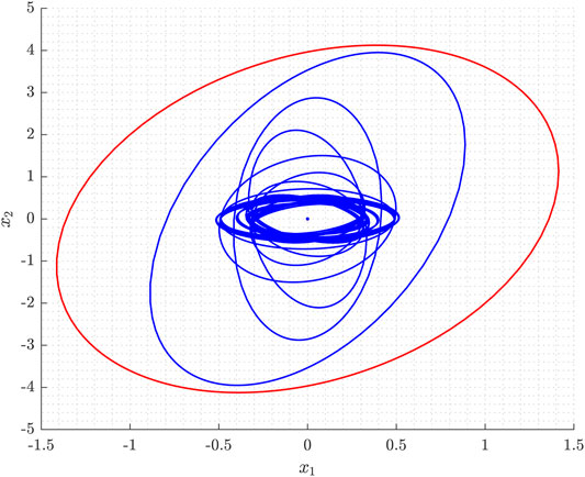
FIGURE 1. Over-approximation of the ellipses corresponding to shape matrices for an arbitrary sequence of discrete states.

Figure 2 illustrates the result of applying the SMPC scheme in the sense of a Markov simulation: The optimization problem Eqs 32–36 is solved repeatedly for sampled realizations of the stochastic variables of the given example. The average computation time for one iteration is about 17.4 ms, i.e. fast enough for online computation. The confidence ellipsoids (blue ellipses) are transferred into the terminal region (green ellipse) over time. For this example, the PRS is guaranteed to contain at least δ_x = 85% of the realizations, but it can be seen that almost every sample (indicated by black stars) lies inside the corresponding PRS. This behavior confirms the conservativeness of the approximation by using the Chebyshev inequality.

FIGURE 2

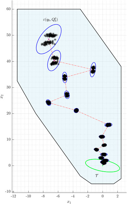
FIGURE 2. Example for n =2: The blue ellipses mark the over-approximated probabilistic reachable sets, the dashed red line indicates the sequence of the expected states, and the green ellipse refers to the target set. The black stars are sampled from a bimodal distribution.

To also demonstrate the applicability of the proposed approach to a JMLS with higher-dimensional continuous state space and more discrete states, next an example with n_z = 8, n = 10, n_u = 6, and a prediction horizon of H = 15 is considered. The matrices A_i, B_i, and G_i were determined randomly. For the initial condition, μ₀ = [1,0,…,0]^T is used, and as in the previous example, x₀ is sampled from a bimodal distribution, obtained from a weighted superposition of two normal distributions parametrized by $q_{\mathrm{0,1}}=19.5\cdot {\underline{1}}^{10,\times ,1}$, $q_{\mathrm{0,2}}=20.5\cdot {\underline{1}}^{10,\times ,1}$, weighted by π₁ = π₂ = 0.5. The corresponding covariance matrices are chosen randomly under the condition that they are symmetric and positive definite. In addition, as in the previous example, the disturbances are chosen uniformly distributed.

The component-wise input and state chance constraints are selected to Pr(|u_i,k| ≤ 5) ≥ 80% and Pr(|x_i,k| ≤ 25) ≥ 80%, and all components of the transition matrix are chosen to p_i,m = 0.125. The average computational time for the determination of the inputs in each time step k is about 124 ms. The results are shown for the different components of x_k over time in Figure 3. The different colors represent these components, for any of which 10 samples are taken. The dashed lines represent the state chance constraints. It is to observe that the presented approach stabilizes any state of this high-dimensional JMLS, while satisfying the chance constraints. The sampled states are far away from the chance constraints, though these are chosen to only δ_x = 80%. As in the first example, this behavior confirms the conservativeness of the Chebyshev approximation. Furthermore, the computational time is low even for larger JMLS, thus enabling the online execution for many real-world systems.

FIGURE 3

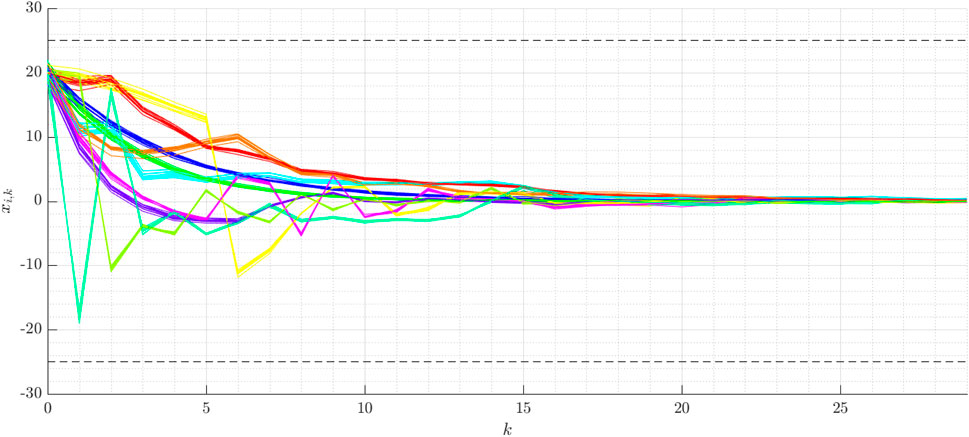
FIGURE 3. Example for the high dimensional JMLS: The different colors represent the components of x_k over the time k.

5 Conclusion

The paper has proposed a method to synthesize a stabilizing control strategy for JMLS with uncertainties, which are modeled as random variables with arbitrarily chosen distributions. The approach can cope with chance constraints for the input and the state. The control strategy is obtained by determining stabilizing feedback control matrices as well as a feasible input sequence by using an MPC-like approach for the conditional expected values. The novel contribution of this paper is to combine the principles of optimization-based controller synthesis and probabilistic reachability for JMLS with arbitrary disturbances, modeled as random variables. Additionally, a method to compute the bounded state covariance matrix for the same system class was derived. In computing the PRS, the use of confidence ellipsoidal sets was motivated by Chebychev estimation. The advantage is, that the PRS of the error part can be computed off-line and together with the tailored formulation of the prediction equations for the expected continuous states, the on-line computational effort of the scheme is relatively low, even for high dimensional Markov systems.

Possible extensions of the proposed technique include the formulation of additional constraints to ensure recursive feasibility, as well as further means to reduce the computational complexity. In addition, in order to avoid the measurability assumptions for the Markov state and the continuous states, the extension of the scheme to state observers may constitute a promising investigation.

Data Availability Statement

The original contributions presented in the study are included in the article/Supplementary Material, further inquiries can be directed to the corresponding author.

Author Contributions

All authors listed have made a substantial, direct, and intellectual contribution to the work and approved it for publication.

Conflict of Interest

The authors declare that the research was conducted in the absence of any commercial or financial relationships that could be construed as a potential conflict of interest.

Publisher’s Note

All claims expressed in this article are solely those of the authors and do not necessarily represent those of their affiliated organizations, or those of the publisher, the editors and the reviewers. Any product that may be evaluated in this article, or claim that may be made by its manufacturer, is not guaranteed or endorsed by the publisher.

Supplementary Material

The Supplementary Material for this article can be found online at: https://www.frontiersin.org/articles/10.3389/fcteg.2022.806543/full#supplementary-material

References

Abate, A., Prandini, M., Lygeros, J., and Sastry, S. (2008). Probabilistic Reachability and Safety for Controlled Discrete Time Stochastic Hybrid Systems. Automatica 44 (11), 2724–2734. doi:10.1016/j.automatica.2008.03.027

CrossRef Full Text | Google Scholar

Asselborn, L., and Stursberg, O. (2016). “Probabilistic Control of Switched Linear Systems with Chance Constraints,” in Europ. Contr. Conf. (ECC), 2041–2047. doi:10.1109/ecc.2016.7810592

CrossRef Full Text | Google Scholar

Asselborn, L., and Stursberg, O. (2015). Probabilistic Control of Uncertain Linear Systems Using Stochastic Reachability. IFAC-PapersOnLine 48, 167–173. doi:10.1016/j.ifacol.2015.09.452

CrossRef Full Text | Google Scholar

Blackmore, L., Bektassov, A., Ono, M., and Williams, B. C. (2007). Robust, Optimal Predictive Control of Jump Markov Linear Systems Using Particles. 05, 4416, 104–117.

Google Scholar

Blackmore, L., Ono, M., Bektassov, A., and Williams, B. C. (2010). A Probabilistic Particle-Control Approximation of Chance-Constrained Stochastic Predictive Control. IEEE Trans. Robot. 26 (3), 502–517. doi:10.1109/tro.2010.2044948

CrossRef Full Text | Google Scholar

Boyd, S., and Vandenberghe, L. (2009). Convex Optimization. New York: Cambridge University Press.

Google Scholar

Cai, Y., and Liu, F. (2007). Constrained One-step Predictive Control of Discrete Time Markovian Jump Linear Systems. Syst. Eng. Elect. 06, 950–954.

Google Scholar

Cheng, J., and Liu, F. (2015). Feedback Predictive Control Based on Periodic Invariant Set for Markov Jump Systems. Circuits Syst. Signal. Process. 34 (8), 2681–2693. doi:10.1007/s00034-014-9936-9

CrossRef Full Text | Google Scholar

Chitraganti, S., Aberkane, S., Aubrun, C., Valencia-Palomo, G., and Dragan, V. (2014). On Control of Discrete-Time State-dependent Jump Linear Systems with Probabilistic Constraints: A Receding Horizon Approach. Syst. Control. Lett. 74, 81–89. doi:10.1016/j.sysconle.2014.10.008

CrossRef Full Text | Google Scholar

Costa, O., Fragoso, M., and Marques, R. (2005). Discrete-Time Markov Jump Linear Systems.

Google Scholar

Costa, O. L. V., Assumpção Filho, E. O., Boukas, E. K., and Marques, R. P. (1999). Constrained Quadratic State Feedback Control of Discrete-Time Markovian Jump Linear Systems. Automatica 35 (4), 617–626. doi:10.1016/s0005-1098(98)00202-7

CrossRef Full Text | Google Scholar

Costa, O. L. V., and Filho, E. O. A. (1996). Discrete-Time Constrained Quadratic Control of Markovian Jump Linear Systems. Proc. 35th IEEE Conf. Decis. Control. 22, 1763–1764.

Google Scholar

Do Val, J. B. R., and Basar, T. (1997). Receding Horizon Control of Markov Jump Linear Systems. Proc. 1997 Am. Control. Conf 55, 3195–3199. doi:10.1109/acc.1997.612049

CrossRef Full Text | Google Scholar

Farina, M., Giulioni, L., and Scattolini, R. (2016). Stochastic Linear Model Predictive Control with Chance Constraints - A Review. J. Process Control. 44, 53–67. doi:10.1016/j.jprocont.2016.03.005

CrossRef Full Text | Google Scholar

Fleming, J., Kouvaritakis, B., and Cannon, M. (2015). Robust Tube MPC for Linear Systems with Multiplicative Uncertainty. IEEE Trans. Automat. Contr. 60 (4), 1087–1092. doi:10.1109/tac.2014.2336358

CrossRef Full Text | Google Scholar

Kamgarpour, M., Summers, S., and Lygeros, J. (2013). “Control Design for Specifications on Stochastic Hybrid Systems,” in Proc. Int. Conf. on Hybrid Systems: Comp. and Contr (ACM), 303–312. doi:10.1145/2461328.2461374

CrossRef Full Text | Google Scholar

Kurzhanskii, A. B., and Vàlyi, I. (1997). Ellipsoidal Calculus for Estimation and Control. Systems and Control : Foundations and Applications. Boston, MA: Birkhäuser.

Google Scholar

Liu, F. (2009). Constrained Predictive Control of Markov Jump Linear Systems Based on Terminal Invariant Sets. Acta Automatica Sinica 34, 496–499. 04. doi:10.3724/sp.j.1004.2008.00496

CrossRef Full Text | Google Scholar

Lu, J., Li, D., and Xi, Y. (2013). Constrained Model Predictive Control Synthesis for Uncertain Discrete‐time Markovian Jump Linear Systems. IET Control. Theor. Appl. 7 (5), 707–719. March. doi:10.1049/iet-cta.2012.0884

CrossRef Full Text | Google Scholar

Lu, J., Xi, Y., and Li, D. (2019). Stochastic Model Predictive Control for Probabilistically Constrained Markovian Jump Linear Systems with Additive Disturbance. Int. J. Robust Nonlinear Control. 29 (15), 5002–5016. doi:10.1002/rnc.3971

CrossRef Full Text | Google Scholar

LygerosCassandras, J. C. G. (2007). Stochastic Hybrid Systems. Taylor & Francis Group/CRC Press. Jan.

Google Scholar

Maciejowski, J. M. (2002). Predictive Control with Constraints. Edinburgh: Prentice-Hall.

Google Scholar

Margellos, K. (2016). “Constrained Optimal Control of Stochastic Switched Affine Systems Using Randomization,” in European Control Conf., 2559–2554. doi:10.1109/ecc.2016.7810675

CrossRef Full Text | Google Scholar

Marshall, A. W., and Olkin, I. (1960). Multivariate Chebyshev Inequalities. Ann. Math. Statist. 31 (4), 1001–1014. doi:10.1214/aoms/1177705673

CrossRef Full Text | Google Scholar

Ogasawara, H. (2019). The Multivariate Markov and Multiple Chebyshev Inequalities. Commun. Stat. - Theor. Methods 49, 441–453. doi:10.1080/03610926.2018.1543772

CrossRef Full Text | Google Scholar

Park, B.-G., Kwon, W. H., and Lee, J.-W. (2001). Robust Receding Horizon Control of Discrete-Time Markovian Jump Uncertain Systems. IEICE Trans. Fundamentals Electronics, Commun. Comp. Sci. 09, 2272–2279.

Google Scholar

Park, B.-G., and Kwon, W. H. (2002). Robust One-step Receding Horizon Control of Discrete-Time Markovian Jump Uncertain Systems. Automatica 38 (7), 1229–1235. doi:10.1016/s0005-1098(02)00017-1

CrossRef Full Text | Google Scholar

Park, B.-G., Lee, J. W., and Kwon, W. H. (1997). Receding Horizon Control for Linear Discrete Systems with Jump Parameters. 36th IEEE Conf. Decis. Control. 44, 3956–3957.

Google Scholar

Schäcke, K. (2004). On the Kronecker Product.

Google Scholar

Tonne, J., Jilg, M., and Stursberg, O. (2015). “Constrained Model Predictive Control of High Dimensional Jump Markov Linear Systems,” in 2015 American Control Conference (ACC), 2993–2998. doi:10.1109/acc.2015.7171190

CrossRef Full Text | Google Scholar

Vargas, A. N., do Val, J. B. R., and Costa, E. F. (2004). Receding Horizon Control of Markov Jump Linear Systems Subject to Noise and Unobserved State Chain. 43rd IEEE Conf. Decis. Control. 44, 4381–4386. doi:10.1109/cdc.2004.1429440

CrossRef Full Text | Google Scholar

Vargas, A. N., do Val, J., and Costa, E. (2005). Receding Horizon Control of Markov Jump Linear Systems Subject to Noise and Unobserved State Chain. 4, 4381–4386.

Google Scholar

Vargas, A. N., Furloni, W., and do Val, J. B. R. (2006). “Constrained Model Predictive Control of Jump Linear Systems with Noise and Non-observed Markov State,” in 2006 American Control Conference, 6. doi:10.1109/acc.2006.1655477

CrossRef Full Text | Google Scholar

Yin, Y., Liu, Y., and Karimi, H. R. (2014). A Simplified Predictive Control of Constrained Markov Jump System with Mixed Uncertainties. Abstract Appl. Anal. 2014, 1–7. Special Issue:. doi:10.1155/2014/475808

CrossRef Full Text | Google Scholar

Yin, Y., Shi, Y., and Liu, F. (2013). Constrained Model Predictive Control on Convex Polyhedron Stochastic Linear Parameter Varying Systems. Int. J. Innovative Comput. Inf. Control. 9 (10), 4193–4204.

Google Scholar