 Tim Kaiser1
 Björn Butter2Samuel Arzt3
 Björn Pannicke2,4
 Julia Reichenberger2,4Simon Ginzinger3
 Jens Blechert2,4*
- 1Clinical Psychology and Psychotherapy, Department of Psychology, University of Greifswald, Greifswald, Germany
- 2Eating Behavior Laboratory, Department of Psychology, Paris-Lodron-University of Salzburg, Salzburg, Austria
- 3MultiMediaTechnology, University of Applied Sciences Salzburg, Salzburg, Austria
- 4Department of Psychology, Centre for Cognitive Neuroscience, Paris-Lodron-University of Salzburg, Salzburg, Austria
Food craving (FC) peaks are highly context-dependent and variable. Accurate prediction of FC might help preventing disadvantageous eating behavior. Here, we examine whether data from 2 weeks of ecological momentary assessment (EMA) questionnaires on stress and emotions (active EMA, aEMA) alongside temporal features and smartphone sensor data (passive EMA, pEMA) are able to predict FCs ~2.5 h into the future in N = 46 individuals. A logistic prediction approach with feature dimension reduction via Best Item Scale that is Cross-Validated, Weighted, Informative and Transparent (BISCWIT) was performed. While overall prediction accuracy was acceptable, passive sensing data alone was equally predictive to psychometric data. The frequency of which single predictors were considered for a model was rather balanced, indicating that aEMA and pEMA models were fully idiosyncratic.
Introduction
Although actual food intake is highly context dependent, for example, on social circumstances, food availability, and meal planning/dieting, food craving (FC) is an internal state that can vary partially independent from actual food intake or hunger (1). FC is defined as an intense desire or urge to consume specific foods (1, 2) that can lead to a loss of control over overeating given fitting circumstances. The high clinical relevance of FCs comes from their central role in binge eating in eating disorders (3). FCs are also related to overeating in obesity (4) and often underlie diet breaches in weight loss dieting (5, 6). FCs are highly contextualized behaviors, meaning that they are triggered in certain situations more so than in others. Thus, FC might be a valuable target for intervention and is the central dependent variable in the present report.
With ecological momentary assessment (EMA), internal states and external contexts that are associated with individual triggers of FCs can be detected (2). EMA is described as the repeated measurement of real-time data in natural environments of individuals (7) and thus can yield intensive longitudinal data with high temporal resolution within the individual. Some further aspects of EMA sampling are also substantial for detecting triggers of FCs: (1) psychometric items can be formalized concerning the present state and context of an individual at the moment of entry, which minimizes retrospective recall bias (8). (2) Repeated measurements of real-time states in real-world environments can record person-specific dynamics (i.e., internal and external states) over time. (3) Besides actively self-reported data (active aEMA, aEMA), EMA designs have the potential to passively collect data (passive EMA, pEMA), such as exact timestamps of data entries or mobile phone sensor data. From timestamps, a multitude of temporal components can be derived, such as intraday rhythms or cycles and global trends across the sampling period (9). In addition, with mobile phone sensors, a wide variety of parameters can be captured, such as app usage, accelerometer, Global Positioning System (GPS) data, screen time, noise, light sensors, etc. These data may not only function as single predictors on their own (10) but can also be aggregated to clusters, representing “virtual situations” that contain information about the environment of participants (11).
Grown from the tradition of ecological momentary interventions, so-called just-in-time adaptive interventions (JITAIs) have recently gained support (12). Such JITAIs can be adapted to specific needs, both in terms of timing and content. Thus, they are provided in situations when individuals need tailored support (13). Moreover, JITAIs are characterized by a data-driven approach, making use of both aEMA and pEMA data types, to allow real-time and context-sensitive interventions (14). Since FCs are sensitive to both, dynamic internal processes and environmental factors and since JITAIs have the potential to capture, combine and react to both, a JITAI approach for FCs seems reasonable. Before implementing a JITAI approach, however, it has to be tested whether future FCs are accurately predictable.
The precision of predicting future FCs may crucially depend on the number and nature of utilized predictors. Further, which type of data is utilized for prediction models has a direct impact on the participant issues, such as burden and compliance. Thus, the present work highlights the distinction between aEMA and pEMA data. We define aEMA as data where the active engagement of a participant is required to answer prompted questionnaires (prompts). aEMA data provide insights into dynamic idiographic subjective-experiential processes that could contain so-called tailoring variables for JITAIs. pEMA is defined as data that contain both temporal facets and mobile phone sensor data, since this can be tracked in the background with a much higher temporal resolution than aEMA data and require minimal participant involvement in the sampling process. Importantly, pEMA data can determine the exact time of events and can capture some aspects of the external context of participants. By combining aEMA and pEMA data, a comprehensive picture of internal and external states emerges, which we refer to as full EMA (fEMA).
The combination of machine learning methods and psychological models allow for the prediction of problematic behavior on a person-specific level. Such behavioral predictions constitute a promising approach for clinical prevention, treatment, and aftercare. Bae et al. (10) were able to differentiate high-risk drinking windows from low-risk windows with an accuracy of 90.9% with solely temporal and mobile phone sensor data as predictors. The results of this and the work of Fisher and Bosley (9) make clear, that cyclic components play a crucial role in modeling idiographic behaviors and states. The classification of low-risk vs. high-risk states from Bae et al. (10) was attained 30 min after drinking onset, thus leaving some time for setting an intervention before drinking gets worse. However, a classification at, or even before the onset of a problematic behavior would be clearly preferable for various other behaviors, where the behavior itself is rather short-lived and preventive measures need to be taken. A so-called time-lagged prediction was implemented by Fisher and Soyster (15) to predict the presence or absence of smoking events in the near future. Such time-lagged models could be the basis of reliable and effective JITAIs, since they allow setting preventive measures for certain risk states.
The current study employed time-lagged predictions of FCs to evaluate the potential feasibility of a future JITAI approach. To do so, we need to estimate the accuracy with which future FC states can be predicted, given a reasonably sized training dataset. Technically, we predicted classes of future FCs in the binary absence (low FC) vs. presence (high FC) separated by an individual threshold because JITAIs need a “decision point” in terminology suggested by Nahum-Shani et al. (14). Conceptually “high FC” would indicate the need for a momentary intervention such as a tip. Additionally, we were interested in contrasting the predictive performance of three distinct predictor ensembles: aEMA (with 18 predictors), pEMA (with 19 predictors), and fEMA (containing all 37 predictors). For model building, we performed Best Item Scale that is Cross-Validated, Weighted, Informative and Transparent [BISCWIT; (16)], since this method allows a minimalized reduction of the predictor space, which prevents overfitting the training data. We expected above-chance prediction of FC classes, though not at the prediction accuracy obtained in alcohol or smoking research as the contextual factors of FCs are potentially more complex and—because FC was measured as a subjective state and is not a directly observable behavior—subject so potentially high measurement error. Lastly, since BISCWIT exerts feature selection, which includes only a subset of available predictors to the model, we were interested in the frequency of selected predictors, reflecting the overall importance of single predictors.
Materials and Methods
Participants
The time series data of participants were drawn from an EMA study on eating behaviors, stress, and emotions. The study was registered at the German register of clinical trials (DRKS ID: DRKS00017493). Participants were included in the study if they were motivated to pursue a conscious diet (N = 184). Participants were randomized to an intervention group receiving daily tips on eating behavior and a control group from which the present sample was drawn (N = 83) based on the use of an android device that provided an adequate amount of sensor data throughout the study to perform clustering procedures. Subjects with an insufficient completion rate of EMA surveys (<50%) were excluded from the study. The resulting sample size was N = 48. Two participants were excluded due to zero variance of reported FCs, leaving a total sample size of N = 46. Across the sampling period of 14 days, retained participants missed on average 14.7 (SD = 11.6) or 17.5% of all 84 prompts (i.e., prompted questionnaires). Participants (82% female) had a mean age of 22.35 years (SD = 2.67) and a mean body mass index (BMI) of 23.22 (SD = 3.02).
Procedure
The study and all procedures were approved by the ethics committee of the University of Salzburg, Austria, and all participants provided informed consent after receiving information on the purpose of the study in oral and written modality prior to data collection.
Active EMA Data Collection
The EMA data collection was carried out using the SmartEater app, which was designed in collaboration with the department of MultiMedia Technology of the University of Applied Sciences Salzburg, Austria. Participants were prompted six times (9 am, 11:30 am, 2 pm, 4:30 pm, 7 pm, and 9:30 pm) each day across 14 days with signals being separated by semi-random time intervals of 150 (±15) min. Thus, a maximum of 84 data points was available for each participant. Participants could respond to the signal up to 60 min after signal onset and rated items either on a horizontal visual analog slider (VAS) from 0 (not at all) to 100 (very much) or with Yes/No statements. For the VAS items, only the extreme values (0 and 100) were labeled. In sum, 18 variables were collected as aEMA: 10 affect-related items orientated on the Positive and Negative Affect Schedule (PANAS) scales (17), three stress and coping-related items based on the Perceived Stress Scale [PSS; (18); German version by (19)], and five food and craving-related items. FCs were measured using the item “How strong is your urge for specific, palatable foods in this moment?” The items were extracted from literature on EMA studies on emotions and eating behavior (20). They were chosen based on comprehensibility, face validity, and a low answering threshold, so that emotions with low intensity are captured as well. Full lists containing all items are provided in Supplemental Materials.
Passive EMA Data Collection and Preparation
The pEMA data consisted of temporal variables and aggregated smartphone sensor data. Temporal components comprised linear, quadratic, and cubic trends computed both for the whole 14 day sampling periods and within days and sinusoidal and cosinoidal ultradian and circadian cycles (9). Additionally, binary time of day variables (e.g., morning, midday, etc.) were derived from prompt numbering. Sensor data included movement data from accelerometer sensors, ambient light recorded by the light sensor of the phone, and ambient noise recorded by the microphone of the phone. Additionally, app usage, push notification, text message, phone call occurrence, and screen time were saved on the device and included in the sensor dataset. The aggregation of mobile phone sensor data into distinct “virtual situations” is described below.
Sensor Aggregation and Clustering
The SmartEater application collected data from a variety of sensors, including accelerometer, audio volume, screen on/off time, and notifications from other applications. In order to find reoccurring patterns in the collected data, the raw sensor values were first aggregated at regular time intervals, which matched the interval of the daily questionnaires presented to users. Before the data of a 1-h interval was aggregated, four sub-intervals of 15 min each were aggregated. Continuous data, such as the accelerometer, audio volume, or screen on/off time, were aggregated in the form of weighted averages, whereas discrete data, such as notifications, were counted. The resulting 4 × 4-dimensional feature space was then reduced to two dimensions using t-distributed stochastic neighbor embedding [t-SNE; (21)], and clusters in the reduced data space were then automatically detected using the spectral clustering (22) with a fixed k-value of 3 [see (23)].
In summary, aEMA data contained 18 variables, pEMA data contained 19 variables (16 temporal and three cluster variables), and fEMA combining both predictor ensembles consisted of 37 variables.
Data Preprocessing
Preprocessing with R version 3.6.1 (24) in R Studio (25) involved missing data imputation for aEMA data using a Kalman filter (26), linear interpolation for respective time differences, z-transformation of predictors, and lagging the FC variable backward for one measurement entry. Thus, for vital time-lagged models, predictors were not associated with the concurrent FC, but with the FC one signal ahead. FCs were dichotomized into classes of high vs. low FC based on the individual mean of the training data. By defining the threshold of dichotomization individually, person-specific response tendencies are taken into account (27).
Idiographic Models Utilizing BISCWIT
The Best Items Scale that is Cross-validated, Unit-weighted, Informative and Transparent [BISCUIT; (28)] is a simple correlation-based machine learning technique. Pairwise correlations between a set of predictors and one or more criterion variables are calculated. The correlations are cross-validated, and predictors with the highest average correlation are retained. Retained predictors are unit-weighted and combined to a sum score. A modification of BISCUIT is BISCWIT. Here, the items are weighted by their correlation with the criterion instead of unit-weighted. Such simple alternatives to more sophisticated machine learning approaches often perform comparable to and sometimes even better, especially when sample sizes and effects are small while measurement error is high (16, 29–31). In this study, BISCWIT was used instead of BISCUIT because correlation-weighted models were more extensively studied and showed more favorable performance in more recent simulation studies (32). Models were computed using the bestScales function, again with 10-fold cross-validation, and correlation-weighted scale scores were obtained by scoreWtd from the psych package (28). The minimum number of selected variables was set to 1, and the maximum number was set to the total number of predictors available for each model.
For statistical models to predict future values of a time series, it is important that they be fit to time-ordered data sets. In this context, the predictive value of statistical models is derived from their accuracy in predicting previously unknown data. Models were thus fit to training data sets that were constructed by taking the first 75% of time series data (i.e., maximum 63 signals, representing 10.5 days). The remaining 25% of time series data (i.e., maximum 21 signals, representing 3.5 days) was used as test data sets. Models were established for (1) aEMA, (2) pEMA, and (3) fEMA data, predicting binary classes of FC. To maximize the reproducibility of our analyses, we set a seed at the beginning of the analysis script. Note that due to the cross-validation approach of BISCWIT, results of single models may vary.
Evaluation of Model Performance
To assess the accuracy of built classifiers, the area under the receiver operating characteristic curve (ROC curve or AUC) was calculated, representing a well-established measure derived from sensitivity and specificity scores across possible cutoff thresholds. Yet, certain aspects of the AUC score can be misleading, such as the unit weighting of omission and commission errors and the evaluation of test performance in extreme ROC regions (33). Thus, we also provide the Brier score, representing the accuracy of probabilistic predictions. While a value of 0.5 was considered as a reference for the AUC, a baseline model for the Brier score constantly predicted the class with the highest occurrence in the training data. A perfect prediction accuracy would result in an AUC value of 1 and a Brier score of 0.
Results
Food Craving
Across the 2-week sampling period, the 46 participants exhibited numeric FCs with a mean of 23.08 (SD = 26.98) ranging from 0 to 100. Individual thresholds (i.e., FC mean of individual subjects), ranging from 5.05 to 58.23 across the sample, were calculated from training data of a participant and were used to categorize both training and test data. FC values above the mean were classified as “high” FC, and values below the mean as “low” FC. Dichotomization based on the mean was chosen because we expected few high-FC states in this non-clinical sample. Other methods of dichotomization (e.g., one SD above the mean) would probably have resulted in too low frequency of these states, making it difficult or even impossible to train a predictive model. Figure 1 depicts the range of frequency of FC means in the sample.
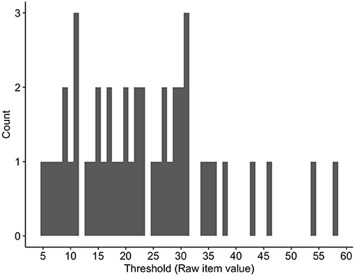
Figure 1. Distribution of individual food craving (FC) thresholds for the whole sample.
Time-Lagged Prediction of Binary Food Craving Classes
For each of the 46 participants, BISCWIT models predicted FC classes ~2.5 h into the future by separately utilizing the three distinct predictor ensembles (aEMA, pEMA, and fEMA). For each participant, the AUC and the Brier score were calculated as measures of classification accuracy. Considering the AUC measure, models outperformed the baseline model with aEMA data in 41 cases (i.e., 89%), with pEMA data in 40 cases (i.e., 87%), and with fEMA data in 39 cases (i.e., 85%). The Brier score yielded comparably lower results: the baseline model was outperformed by aEMA data in 32 cases (i.e., 70%), by pEMA data in 21 cases (i.e., 46%), and by fEMA data in 32 cases (i.e., 70%).
To assess the overall prediction accuracy, Table 1 shows the mean prediction accuracy for each predictor ensemble across all 46 participants.

Table 1. Accuracy of predictor ensembles in predicting food craving classes.
Furthermore, within-subject variability was found regarding which predictor ensemble classifies best. Consequently, variability of which predictor type is preferred for classification is also found at an aggregated level, across all participants. Figure 2 depicts this variability showing exemplary results from five participants. This illustrates the highly idiosyncratic nature of FC prediction.
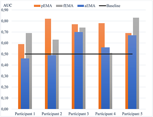
Figure 2. Exemplary AUC scores for aEMA, pEMA and fEMA data obtained from 5 participants.
Feature Selection
The BISCWIT employs feature selection by selecting the best predictors based on cross-validated raw correlations. Tables S2–S4 show how often the included variables were selected as predictors for each model across all participants. For all models, each variable was selected within a range of 2 to 31 times. Within each predictor ensemble, none of the variables was overrepresented. Table 2 shows the average number of predictors that were considered for each model.
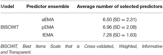
Table 2. The average number of selected predictors for BISCWIT models across 46 participants.
Discussion
Although FCs play a key role in enhancing problematic eating behaviors (4), the present study is the first to establish idiographic time-lagged models to test whether their prediction into the future is feasible and acceptably accurate for a JITAI application. To remedy that, time series data of 46 healthy participants motivated for weight loss were drawn from an EMA study on eating behaviors, stress, and emotions. For each participant, three prediction models were established, utilizing either aEMA, pEMA, or fEMA data for the prediction of FC classes. Importantly, all models were time-lagged, meaning that each prediction referred to the upcoming signal (roughly 150 min into the future). Furthermore, models were built on training data, and out-of-sample generalizability was assessed on test data. It was hypothesized that FC states of upcoming signals can accurately be predicted, and that predictor ensembles differ in precision. Due to the fully individualized FC prediction method, we cannot provide a mechanistic or theoretical explanation for the observed relationship between certain sensor clusters and FC. This is in line with the highly individual pattern of craving states. According to conditioning accounts (34), FC occurs in situations that were paired with palatable food intake in the past. Situational influences on FCs are highly idiosyncratic. It was not the intention of this study to derive a generalizable pattern of craving predictors but to depart from this in building individualized machine learning models that allow the prediction of individual FC patterns.
Prediction Accuracy of Predictor Ensembles (aEMA, pEMA, and fEMA)
The pragmatic goal of contrasting distinct predictor ensembles was to show how accurate pEMA data, which require minimal sampling effort, can predict FCs compared to aEMA/fEMA, which requires substantially more sampling effort, especially for longer sampling periods and higher sampling frequencies. On average, all models outperformed the baseline models; however, neither aEMA, pEMA, nor fEMA models differed in their precision. This finding implies that on average pEMA data perform comparably to fEMA; therefore, aEMA adds no additional precision for predicting FCs. For studies that solely aim for precision accuracy, aEMA could be left out, which lowers participant burden and thus may increase compliance. This result also corresponds with existing findings that FC is associated with both, internal psychological states (aEMA) and certain contextual factors and follows temporal patterns (pEMA) (2). On an idiographic level, however, we saw that it can make crucial differences regarding which ensemble (e.g., aEMA or pEMA) is used for FC prediction (as indicated by Figure 2). This represents an unexpected variability regarding which ensemble is preferred within each participant. Further research could detect differences between certain population groups for whom aEMA and for whom pEMA predicts FCs best. For example, personality traits could moderate the extent to which FCs are triggered by internal processes vs. external contexts. Note that also in other research areas such as substance use, differences regarding the prediction performance of aEMA and pEMA are to date unexplored. In this study, aEMA data included mainly affect- and stress-related items. Future studies could further improve the precision of aEMA data by examining a broader set of predictors, validating and expanding them by involving stakeholders (35). Similarly, the set of pEMA predictors could be expanded by including a wider variety of sensor data, possibly adding physiological measures like heart rate or skin conductance response. By using techniques like the Lombard–Scargle periodogram, more individualized cyclic temporal predictors could be extracted directly from psychometric time series.
Prediction Accuracy and Feature Selection of BISCWIT
The BISCWIT originates from nomothetic personality research and is used, to the best knowledge of authors, for the first time for idiographic prediction models. BISCWIT was chosen, since some models had a statistically questionable feature-to-observation ratio (e.g., 37 predictors with 50 observations), which required a dimensionality reduction of the feature space. BISCWIT aggregated the cross-validated best predictors of FC into a single scale, leaving a maximally parsimonious model with a single predictor. Since BISCWIT exerts feature selection, we investigated the variables selected by the models as contributing non-redundant information to the prediction. The fact that the frequency at which each variable was considered for a model seemed evenly distributed (see Tables S2–S5) suggests that each participant has its own unique set of variables predicting FC. Therefore, it was not possible to identify key predictors among all 37 available variables. Scientifically, this is noteworthy: it actually suggests that there is no generalizable pattern in variable importance, but prediction models are fully idiosyncratic. The constellation of variables being important for craving prediction of participant 1 allows no extrapolation to the potential constellation in participant 2. It is also noteworthy that the presence or absence of a specific virtual cluster from mobile phone sensor data did also contribute to predicting FCs. Thus, high-dimensional mobile phone sensor data can be aggregated to meaningful, virtual clusters that are associated with internal subjective states and behaviors (11, 23). This comes with the clear advantage of gathering predictive variables in the background, without increasing participant burden. Additionally, it is worth mentioning that global trend variables were frequently considered as predictors, which indicates non-stationarity in some time series data and could reflect one reason why estimates for out-of-sample data were rather imprecise (9).
Note that further prediction algorithms than BISCWIT were also performed in this study (Elastic Net Regression and Support Vector Machines). Since their results did not surpass BISCWITs precision (see Tables S4, S5), the focus remained on the simplest algorithm.
Practical Implications and Limitations of the Study
Although models for some participants exhibited almost perfect classification scores (AUC scores of 0.8–1.0), the overall above chance information within predictions remains low relative to other behaviors and maybe too low for a real-world JITAI application. This lack of prediction accuracy may be the result of the following two considerations: (a) the interval of 2.5 h between questionnaire prompts could be too wide to allow models detecting temporal lagged relationships between predictors at t1 and FCs at t2 and (b) this study predicted an internal state measured by a single item, which may lead to an unwanted signal-to-noise ratio. As a consequence, more accurate predictions could be obtained by considering multiple aspects of FC instead of one single item. Further research is needed to determine individually and a priori which type of data might produce the highest prediction accuracy and for whom a time-lagged prediction in general works. Similar to the prediction of mood profiles (9), FC profiles could be generated by employing established instruments such as the Food Craving Questionnaire (36) or predicting a score calculated from such questionnaires. Also, a sampling period exceeding 14 days would provide more within-person data for prediction algorithms to make better estimates of future FCs, but would, of course, increase burden.
The present study separated classes of FCs using the individual mean, which accounts for personalization and individual differences in response behavior. However, and since we analyzed healthy participants, we cannot claim that such a threshold can differentiate between the absence and presence of a clinical risk state as, for example, uncontrolled binge eating. The definition of a threshold that indicates the need for a personalized intervention has to be empirically validated, especially for clinical participants. The results of this work suggest, that no predictor ensemble outperforms the other in overall prediction accuracy of FC. As a consequence, researchers may decide whether aEMA or pEMA data should be sampled depending on whether participant burden should be minimized or on other technical requirements and data processing steps. Pragmatically, the present results suggest that pEMA would be sufficient for acceptable predictions in just about half of the participants.
Conclusion
Results of the present work demonstrate that a time-lagged prediction of FC classes, in general, is feasible. We found that aEMA does not provide any additional accuracy over pEMA data and that simple models such as BISCWIT can be considered for high-dimensional data. A challenge for future research would be combining individual prediction models with theory based, between person predictors such as age, gender, BMI, or trait-level emotional eating scores or FC as done in multilevel-based prediction models (20, 37).
Data Availability Statement
The raw data supporting the conclusions of this article will be made available by the authors, without undue reservation.
Ethics Statement
The studies involving human participants were reviewed and approved by Ethics Committee of the University of Salzburg. The patients/participants provided their written informed consent to participate in this study.
Author Contributions
TK and BB analyzed and interpreted the data and wrote the manuscript. SA analyzed and interpreted the data. BP and JR designed the study and collected the data. SG supervised the study. JB designed and supervised the study and wrote the manuscript. All authors contributed to the article and approved the submitted version.
Funding
This work was supported in whole, or in part, by the Austrian Science Fund (FWF)[KLI 762.B]. In addition, funding was received from the European Research Council (ERC) under the European Union's Horizon 2020 research and innovation program (ERC-PoC-2018 825403 SmartEater).
Conflict of Interest
The authors declare that the research was conducted in the absence of any commercial or financial relationships that could be construed as a potential conflict of interest.
Publisher's Note
All claims expressed in this article are solely those of the authors and do not necessarily represent those of their affiliated organizations, or those of the publisher, the editors and the reviewers. Any product that may be evaluated in this article, or claim that may be made by its manufacturer, is not guaranteed or endorsed by the publisher.
Supplementary Material
The Supplementary Material for this article can be found online at: https://www.frontiersin.org/articles/10.3389/fdgth.2021.694233/full#supplementary-material
References
1. Weingarten HP, Elston D. Food cravings in a college population. Appetite. (1991) 17:167–75. doi: 10.1016/0195-6663(91)90019-O
2. Reichenberger J, Richard A, Smyth JM, Fischer D, Pollatos O, Blechert J. It's craving time: time of day effects on momentary hunger and food craving in daily life. Nutrition. (2018) 55–56:15–20. doi: 10.1016/j.nut.2018.03.048
3. Moreno S, Warren CS, Rodríguez S, Fernández MC, Cepeda-Benito A. Food cravings discriminate between anorexia and bulimia nervosa. Implications for “success” versus “failure” in dietary restriction. Appetite. (2009) 52:588–94. doi: 10.1016/j.appet.2009.01.011
4. Verzijl CL, Ahlich E, Schlauch RC, Rancourt D. The role of craving in emotional and uncontrolled eating. Appetite. (2018) 123:146–51. doi: 10.1016/j.appet.2017.12.014
5. Meule A, Küppers C, Harms L, Friederich, H.-C., Schmidt U, et al. Food cue-induced craving in individuals with bulimia nervosa and binge-eating disorder. PLoS ONE. (2018) 13:e0204151. doi: 10.1371/journal.pone.0204151
6. Fedoroff I, Polivy J, Peter Herman C. The specificity of restrained versus unrestrained eaters' responses to food cues: general desire to eat, or craving for the cued food? Appetite. (2003) 41:7–13. doi: 10.1016/S0195-6663(03)00026-6
7. Shiffman S. Conceptualizing analyses of ecological momentary assessment data. Nicotine Tobacco Res. (2014) 16(Suppl. 2):S76–87. doi: 10.1093/ntr/ntt195
8. Engel SG, Crosby RD, Thomas G, Bond D, Lavender JM, Mason, et al. Ecological momentary assessment in eating disorder and obesity research: a review of the recent literature. Curr Psychiatry Rep. (2016) 18:1–9. doi: 10.1007/s11920-016-0672-7
9. Fisher AJ, Bosley HG. Identifying the presence and timing of discrete mood states prior to therapy. Behav Res Ther. (2020) 128:103596. doi: 10.1016/j.brat.2020.103596
10. Bae S, Chung T, Ferreira D, Dey AK, Suffoletto B. Mobile phone sensors and supervised machine learning to identify alcohol use events in young adults: implications for just-in-time adaptive interventions. Addict Behav. (2018) 83:42–47. doi: 10.1016/j.addbeh.2017.11.039
11. Beierle F, Tran VT, Allemand M, Neff P, Schlee W, Probst T, et al. Context data categories and privacy model for mobile data collection apps. Procedia Comput Sci. (2018) 134:18–25. doi: 10.1016/j.procs.2018.07.139
12. Wang L, Miller LC. Just-in-the-Moment Adaptive Interventions (JITAI): a meta-analytical review. Health Commun. (2019) 35:1531–44. doi: 10.1080/10410236.2019.1652388
13. Nahum-Shani I, Hekler EB, Spruijt-Metz D. Building health behavior models to guide the development of just-in-time adaptive interventions: a pragmatic framework. Health Psychol. (2015) 34:1209–19. doi: 10.1037/hea0000306
14. Nahum-Shani I, Smith SN, Spring BJ, Collins LM, Witkiewitz K, Tewari A, et al. Just-in-Time Adaptive Interventions (JITAIs) in mobile health: key components and design principles for ongoing health behavior support. Ann Behav Med. (2018) 52:446–62. doi: 10.1007/s12160-016-9830-8
15. Fisher AJ, Soyster PD. Generating accurate personalized predictions of future behavior: a smoking exemplar. (2019). doi: 10.31234/osf.io/e24v6
16. Elleman LG, McDougald SK, Condon DM, Revelle W. That takes the BISCUIT. Eur J Psychol Assess. (2020) 36:948–58. doi: 10.1027/1015-5759/a000590
17. Watson D, Clark LA. Development and validation of brief measures of positive and negative affect: the PANAS scales. J Pers Soc Psychol. (1988) 54:1063–70. doi: 10.1037/0022-3514.54.6.1063
18. Cohen S, Kamarck T, Mermelstein R. A global measure of perceived stress. J Health Soc Behav. (1983) 24:385–396. Available online at: https://doi.org/10/d2wgms
19. Büssing A, Günther A, Baumann K, Frick E, Jacobs C. Spiritual dryness as a measure of a specific spiritual crisis in catholic priests: associations with symptoms of burnout and distress. Evid Based Complement Alternat Med. (2013) e246797. doi: 10.1155/2013/246797
20. Reichenberger J, Kuppens P, Liedlgruber M, Wilhelm FH, Tiefengrabner M, Ginzinger S, et al. No haste, more taste: an EMA study of the effects of stress, negative and positive emotions on eating behavior. Biol Psychol. (2018) 131:54–62. doi: 10.1016/j.biopsycho.2016.09.002
22. von Luxburg U. A tutorial on spectral clustering. Stat Comput. (2007) 17:395–416. doi: 10.1007/s11222-007-9033-z
23. Arzt S, Ginzinger S. Fine-grained daily routine detection from smartphone usage and sensor data (2021).
24. R Core Team. R: A Language and Environment for Statistical Computing. R Foundation for Statistical Computing (2020). Available online at: https://www.R-project.org/
25. RStudio Team. RStudio: Integrated Development for R. Boston, MA: MARStudio, Inc. (2015). Available online at: http://www.rstudio.com/
27. Batchelor JH, Miao C. Extreme response style: a meta-analysis. J Organ Psychol. (2016) 16:51–62.
28. Revelle W. psych: Procedures for Personality and Psychological Research. Evanston, IL: Northwestern University (2021). Available online at: https://CRAN.R-project.org/package=psych Version = 2.1.6.
29. Dana J, Dawes RM. The superiority of simple alternatives to regression for social science predictions. J Educ Behav Stat. (2004) 29:317–31. doi: 10.3102/10769986029003317
30. Dawes RM. The robust beauty of improper linear models in decision making. Am Psychol. (1979) 34:571–82. doi: 10.1037/0003-066X.34.7.571
32. Waller NG, Jones JA. Correlation weights in multiple regression. Psychometrika. (2010) 75:58–69. doi: 10.1007/s11336-009-9127-y
33. Lobo JM, Jiménez-Valverde A, Real R. AUC: a misleading measure of the performance of predictive distribution models. Glob Ecol Biogeogr. (2008) 17:145–51. doi: 10.1111/j.1466-8238.2007.00358.x
34. Martin CK, McClernon FJ, Chellino A, Correa JB. Food cravings: A central construct in food intake behavior, weight loss, and the neurobiology of appetitive behavior. In: Preedy VR, Watson RR, Martin CR editors, Handbook of Behavior, Food and Nutrition. Springer (2011) 741–755.
35. Soyster PD, Fisher AJ. Involving stakeholders in the design of ecological momentary assessment research: an example from smoking cessation. PLoS ONE. (2019) 14:e0217150. doi: 10.1371/journal.pone.0217150
36. Nijs IMT, Franken IHA, Muris P. The modified trait and state food-cravings questionnaires: development and validation of a general index of food craving. Appetite. (2007) 49:38–46. doi: 10.1016/j.appet.2006.11.001
37. Reichenberger J, Pannicke B, Arend, A.-K., Petrowski K, Blechert J. Does stress eat away at you or make you eat? Ema measures of stress predict day to day food craving and perceived food intake as a function of trait stress-eating. Psychol Health. (2020) 36:129–47. doi: 10.1080/08870446.2020.1781122
Keywords: food cravings, time-lagged, idiographic models, BISCWIT, ecological momentary assessment, passive sensing, mobile health, eating behavior
Citation: Kaiser T, Butter B, Arzt S, Pannicke B, Reichenberger J, Ginzinger S and Blechert J (2021) Time-Lagged Prediction of Food Craving With Qualitative Distinct Predictor Types: An Application of BISCWIT. Front. Digit. Health 3:694233. doi: 10.3389/fdgth.2021.694233
Received: 12 April 2021; Accepted: 17 August 2021;
Published: 20 September 2021.
Edited by:
Matthew Crowson, Massachusetts Eye & Ear Infirmary and Harvard Medical School, United StatesReviewed by:
Laura Maria König, University of Bayreuth, GermanyJinhyuk Kim, The Pennsylvania State University (PSU), United States
Copyright © 2021 Kaiser, Butter, Arzt, Pannicke, Reichenberger, Ginzinger and Blechert. This is an open-access article distributed under the terms of the Creative Commons Attribution License (CC BY). The use, distribution or reproduction in other forums is permitted, provided the original author(s) and the copyright owner(s) are credited and that the original publication in this journal is cited, in accordance with accepted academic practice. No use, distribution or reproduction is permitted which does not comply with these terms.
*Correspondence: Jens Blechert, jens.blechert@sbg.ac.at