Was Thebes Necessary? Contingency in Spatial Modeling

1. Introduction

Data are never perfect. However, when they are good, as is often the case in the physical sciences, there are various programmes for tackling data deficiency (e.g., Kennedy and O’Hagan, 2001; Babtie et al., 2014). In social science, and in archeology in particular, data are often too poor for these approaches to be applicable as they stand. The information we have is incomplete and fragmentary, biased by what has survived and by what has been investigated and what has been made publicly available. We have to supplement the data that we possess with informed guesswork of various levels of detail and reliability. In the light of this, to make the best use of our limited knowledge or, complementarily, the best use of our ignorance a good starting point is to adopt the fall-back position of answering the question “All other things being equal, I would expect … to have happened?”

This is where modeling can add to the debate. How to make the best use of our ignorance is an old problem and we shall not attempt to document its history much beyond the observation that economists, who popularized the approach in the 20th century, refer to it [see (Keynes, 1921), chapter 4] as Laplace’s “Principle of Indifference,” although Laplace himself termed it the “Principle of Insufficient Reason” (Laplace, 1825). However named, the basic idea (which precedes Laplace) is simple in principle and is exactly how a wise card player would have played at the gambling tables of the ancient regime. List all the “worlds” (in this case, hands of cards), which are compatible with your knowledge/ignorance. Each world is equally likely (or information is being withheld), and the most typical of these is the way in which the system is most likely to behave. In the language of Bayesian statistics (Laplace’s analysis rather subsumed the ideas of Bayes, but it is Bayes whose name is invoked by statisticians), we have assumed a flat Bayesian prior. Necessarily our conclusions will have a large degree of uncertainty about them, and our main aim in this article is to attempt to show how this uncertainty can be estimated.

There is a basic issue here that sets us, as archeologists, apart from historians, particularly where data are poor. This is that modeling of the type that we are discussing applies only to generic societal behavior, behavior that arises when “history is idling.” While it is easy to discount the historical staples of major social unrest, famine, and disease, it is less easy to estimate those aspects of local alliances that lead to one decision rather than another. That is, in the context of the above, we are less interested in an enraged gambler overthrowing the table than in the presence of organized card sharps. To take the example of this paper that we shall develop at greater length later, the formation of Greek city-states in ninth and eight century BC, we shall see that there is a contingency to the presence of Thebes that does not apply to Athens. Indeed, it is hard to get Thebes to appear as a major site. We would see this as a consequence of social forces (not necessarily dramatic) that modeling of this type, based on the broad statistical inference, cannot accommodate. Although to a historian the absence of Thebes in its historical position is nonsense, a Bayesian is happy with a local proxy, which differs in detail and position from the original, provided something sensible is said about Athens, Korinth, and other important sites.

Jaynes (1957, 1973) reformulated the Bayes/Laplace approach as the Principle of Maximum Ignorance (or Principle of Epistemic Modesty), and this is the view closest to the methods we will use in this work, in that it can be reformulated as the Principle of Maximum Entropy. Here, we are thinking of entropy in the context of information theory, in which it is simply related to the number of questions with which we need to interrogate the system to have complete knowledge of it. Maximum entropy states are, roughly speaking, the ones that have the largest number of ways of creating a result with the specified macroscopic observables (our limited knowledge), and this fits in with Bayes/Laplace. As always, there are certain caveats that we shall not address and leave to the interested reader (Neapolitan and Jiang, 2014).

Our focus here is on models for networks of exchange in the protohistoric past where the primary information contained in the model is spatial. Our worlds are patterns of exchange, and a typical use of such models is to see to what extent spatial features alone can account for these. The entropy maximizing that we shall discuss here is only one of several approaches that have evolved in part from urban planning, migration/commuting, and economics, for all of which exchange is a key component. We have delineated some of the alternative lines of approach elsewhere (Evans et al., 2012) and will not pursue them further.

To examine the issues with quantifying levels of expectation with their concomitant uncertainty and ambiguity, we will build on a classic study using entropic methods demonstrated by Rihll and Wilson (1987, 1991). They examined how spatial models, based on models for siting retail outlets (Huff, 1964; Lakshmanan and Hansen, 1965; Harris and Wilson, 1978), can be used to study the rise of city-states in central mainland Greece around the eighth century BC. Specifically, the question is to understand to what extent spatial features can explain why certain settlements out of the many in the region came to dominate it. The success of the model led to its adoption for understanding city-state formation in other times and other places: second millennium BC Crete (Bevan and Wilson, 2013), Middle Bronze Age and Iron Age NE Syria (Davies et al., 2014), early second millennium BC Central Anatolia (Palmisano and Altaweel, 2015), and late first millennium Latenian urbanization (Filet, 2017).

Our aim is, using the data of Rihll and Wilson as the example, to show how to improve the treatment of uncertainty in such spatial modeling. This lies behind the title of this article. We shall show that some sites, like Athens, are likely to be significant despite our poor knowledge, whereas some, like Thebes, are much more contingent on information that we do not possess. Unlike Athens, its historical importance is likely a consequence of social forces that models like ours cannot accommodate. We had suggested this previously (Rivers and Evans, 2014), and this current article provides an extensive development and analysis of this earlier proposition. However, our focus in this article is less on the archeology of Late Geometric/Early Archaic Greece (Coldstream, 2003) and more on the nature of uncertainty in such approaches. As such it is equally applicable to the other case studies, and some preliminary work on Latenian urbanization is under way.

As we have said, these studies of urbanization are framed in the language of exchange networks. In the first instance, “exchange” means the physical transportation of things and people, with secondary meanings in terms of power and culture that these things and people embody, the details of which we know very imperfectly. Uncertainty comes in many forms, but, roughly, it can be divided into uncertainty in “physical” parameters and uncertainty in “calibration” (Kennedy and O’Hagan, 2001). For the former, a major source of uncertainty lies in our imperfect knowledge of site locations. In this regard, we take the sites of the Rihll and Wilson model as given. Even then, further uncertainty lies in the nature of the paths taken (we are thinking here of land-based and riverine travel), e.g., to what extent do existing roads and waterways determine long-distance exchange? We consider the effect of adopting different definitions. A third problem arises in estimating the effort/cost/time involved in the transportation along these routes. These, in addition to the ambiguity in the site carrying capacities or resource bases, constitute the major uncertainties in the physical parameters of the model. As for calibration, there is the question of how to characterize the ease of exchange for different “costs” or distances. This is encoded in the so-called deterrence function, a calibration function, with its own calibration parameters, which imposes cost penalties on long-distance single transactions. We consider the effect of different choices of this deterrence function. In fact, what began our analysis of this data set (Rivers and Evans, 2014) was our inability to replicate the results of Rihll and Wilson when using a different choice of deterrence function from them.

Superficially, our conclusions concerning significant sites seem very plausible just on geometric grounds from the distribution of sites. This leads us to question whether we needed the apparatus of entropy and Bayesian analysis. Could we have reached good enough conclusions with a ruler and compass? To test such a null approach, we compare the results of this model to the results obtained using more traditional data clustering methods, which rely on geography alone. We find that the answer is no. As a part of this programme, we produce an open source list of site locations and distances used, which allows future researchers to test their ideas on this data set.

There is the caveat that even seemingly epistemic approaches like this can have a manifestly ontic realization in terms of sites as actors in their evolution. For example, Wilson (2008) rephrases the model in terms of dynamical Lokta–Volterra (predator–prey) equations, and Altaweel (2015) has re-examined Syrian city-state formation from an agent-based approach. Such approaches provide useful complementary perspectives.

2. Data

2.1. Sites

The primary data we use is that of Rihll and Wilson (1991) (pp. 68–71), namely the choice and location of sites. The sites chosen come from a region roughly 130 km across from the Greek mainland as shown in Figure 1. The sites used constitute 109 population centers of the Late Geometric period, the ninth and eight century BC, as specified in Figure 1 of the study by Rihll and Wilson (1987) and shown here in Figure 2. We assign the same index to each site as in the study by Rihll and Wilson (1987), and this index will be given in the text along with the site name. A full list of site names and indices is given in the Table A1 in Appendix or see Evans (2016a) for full details.

FIGURE 1

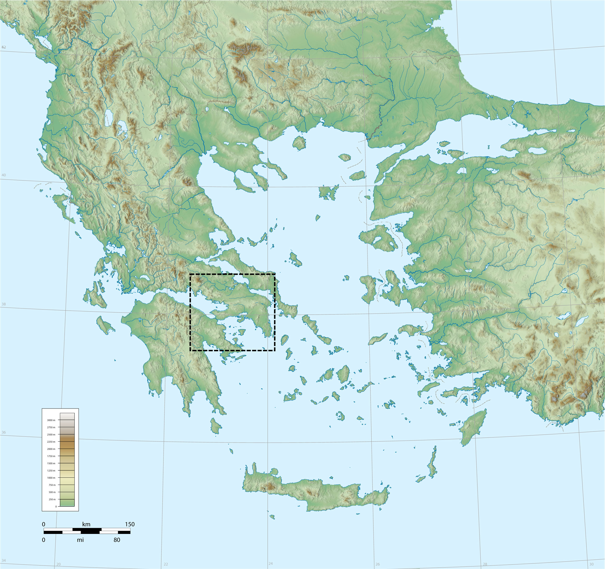
Figure 1. Mainland Greece and the Aegean. The box shows the region containing the 109 sites of Rihll and Wilson [Figure 1 of Rihll and Wilson (1987)], which are used in the analysis here, see Figure 2. Map from Wikipedia Commons.

FIGURE 2

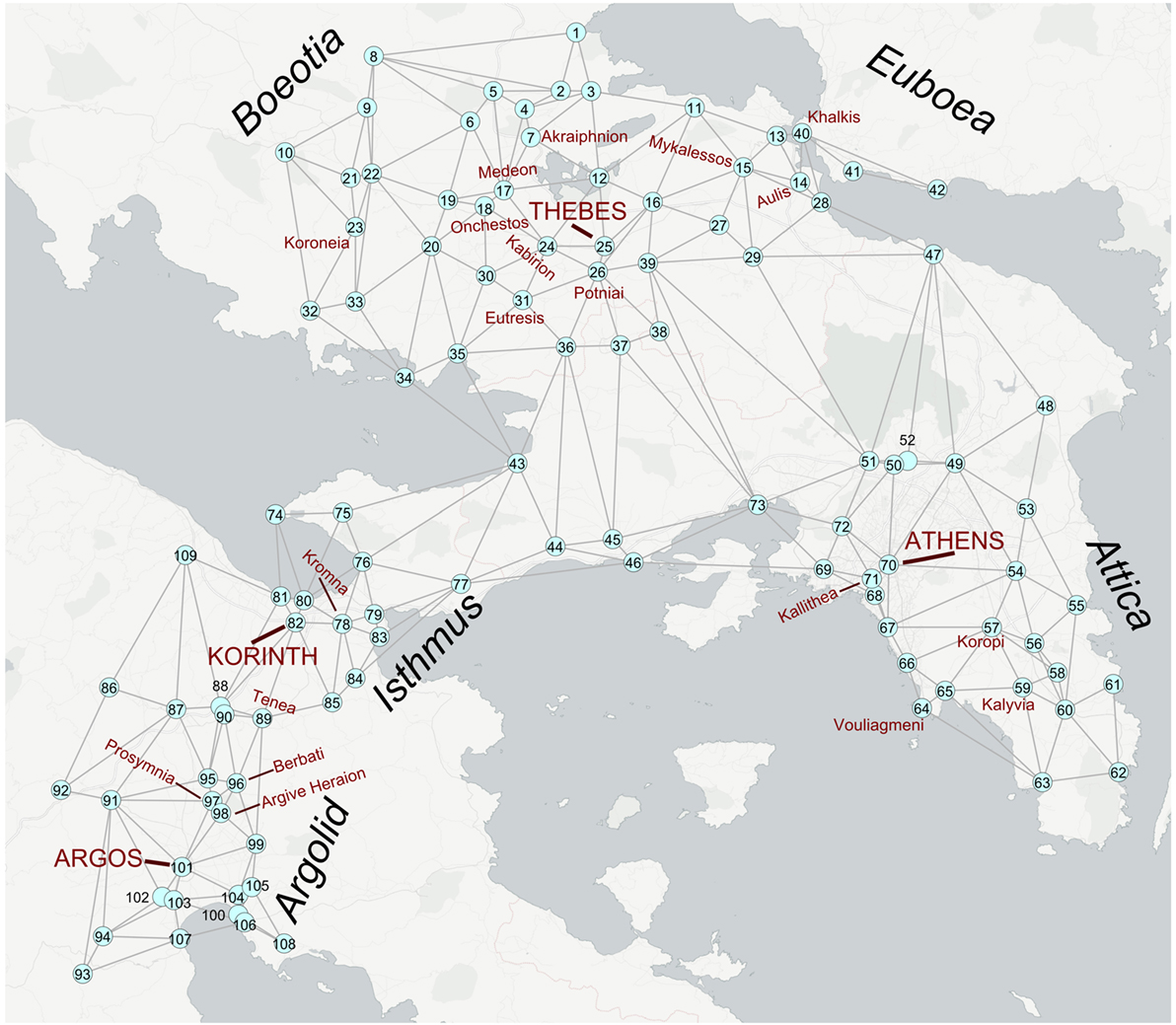
Figure 2. The approximate locations of the 109 sites used as the starting point for this study, derived from Figure 1 of Rihll and Wilson (1987). The index of each site is the same as in the study by Rihll and Wilson (1987) and is indicated by the number on the associated site. These indices are used in the text, usually in parentheses after the site name. The index of site numbers and the precise locations used in this study are given in full in Table A1 in Appendix along with this map using site names not site indices (Figure A1 in Appendix). Note that site 64, Vouliagmeni, was not labeled in the original figure; see Evans (2016a) for more details. The “normal” distance set are the direct straight line distances between these sites. The edges are a subset of those given by Delaunay Triangulation and are used to calculate a second set of distances (denoted DTMedit). Each edge is linked to the straight distance between the end points. The distance between other pairs of points is found by taking the length of the shortest path along the edges where the path distance is the sum of the distances associated with the edges traversed in the path. The full data set and further details are given in the study by Evans (2016a).

Some of the hypotheses behind the choices of sites are outlined in the study by Rihll and Wilson (1987), e.g., using the existence of a temple or the size of a site as a marker of importance. Relying on such expert judgment is inevitable, but this approach immediately provides a largely unquantifiable source of uncertainty. Inevitably, some sites will be missing from the current archeological record, a gap that is difficult to fill without modeling. One systematic approach to such missing sites is to take a subset of existing sites and a knowledge of the geography. Extra sites are then added using some stochastic model, and results are then produced for this mixture of real and artificial sites. Repeating this many times for many possible missing site configurations will allow us to see whether we can draw any general conclusions about our system independent of our uncertainty about sites; Bevan and Wilson (2013) or Paliou and Bevan (2016) provide examples of this procedure. Another approach to the uncertainty around our selection of sites could be to try different random subsets of known sites. Again repeating measurements several times will allow us to judge how site location uncertainty effects our conclusions, for example, see the study by Davies et al. (2014).

A further judgment comes when we draw the boundary. The 109 sites chosen here lie within about a days walk from one of the four key centers: Argos, Korinth, Thebes, and Athens. This provides one rationale for the boundary of the region considered here. However, there are clearly strong links in this period between the sites in this study and the wider Greek world (Coldstream, 2003): Thessaly, Sparta and the rest of the Peloponnese, the Aegean islands, colonies founded in Sicily, and elsewhere. Commerce provided vital links with Italy and the Eastern Mediterranean for key ores if nothing else (Coldstream, 2003). In principle, we could look to include more and more sites in our study.

However, in this work, we will not try to address such uncertainties in the choice of sites, and we will take the set of 109 sites in Figure 2 as given. See the study by Evans (2016a) for these data and further information on our implementation of this information.

Some models can accommodate some sense of the size of the site. However, Rihll and Wilson judge that this information is very uncertain in this period, and it is more reasonable to assume that all sites were roughly equal in size and importance at the start of the period [see Rihll and Wilson (1991) (pp. 69–70)]. This reflects an entropy viewpoint that this is the least-biased assumption to make when there is no other information available.

There is one obvious feature about the spatial arrangement of these 109 sites. There is a natural and obvious division into three regions: Boeotia, Attica, and the Isthmus-Argolid region. We will comment further on the properties of the spatial arrangement of these 109 sites below, see Section 2.3.

2.2. Distances

The only other explicit information used here, and in the original papers, is the distance between every pair of sites [see Rihll and Wilson (1991), pp. 63–65]. There are many different ways to assess the effective separation of two sites: effort, time of travel, financial costs, distance of the actual route followed, etc. For our context, only the distance of the actual route followed can be measured with any accuracy using modern GIS methods, but lack of knowledge about the details of exchange and the way landscapes were actually used still leaves unquantifiable uncertainties. Again the best response is to make few assumptions, so in the first instance, like Rihll and Wilson, we use a straight line distance between sites. In fact the choice of significant sites may well contain some implicit information about the landscape, e.g., an area of difficult terrain is likely to have fewer settlements. We will try to judge the effect of the uncertainty of distance as a part of our study, one aspect where we extend the original work of Rivers and Evans (2014).

One complication when comparing our results to the original studies is that the distances used in the latter are not provided. To obtain a comparable set of distances, we have digitized Figure 1 of Rihll and Wilson (1987); our coordinates for the sites are given in the Table A1 in Appendix. The distance between sites is then the length of a straight line between these sites in these coordinates. This comprises what we will call our “normal” distance data set. These distance data are given in the study by Evans (2016a), and the process is discussed there in more detail. The scale is that roughly six of our units are equivalent to 1 km. If we look at the nearest neighbor to each site, we find that the closest pair are 8 U apart (Nauplia—106, Pronaia—100, and south east of Argos—101), and the furthest distance between nearest neighbors is 75 U (between Sikyon—109 and Akraia—74 on the coast north of Korinth—82). These minimum distances have a first quartile of 20.0, a median of 28 (such as Kopai—5 and Olmous—6 in northern Boeotia), and a third quartile of 39.0. The mean is 30.9 U implying a short distance scale of around 5 km.

Perhaps the most obvious problem with these data is that the shortest path between many pairs of points includes paths that are over the sea. Traveling on water in the ancient world was, where it was available, the most effective method of long-distance communication, both in terms of speed and in terms of bulk. However, land-borne and waterborne transports have different advantages and disadvantages meaning that we cannot simply mix these two modes of travel. This issue largely affects long-range links across our region. We shall see later that the bulk of the results seem to be sensitive to smaller scales, say 30 km or less (the maximum walking distance in 1 day). We might reasonably hope that sea travel is likely to have little impact on our results and have used this to produce a second set of separations based purely on routes that (largely) avoid the open sea.

From the above, we see sites are so close that a determined individual could visit several sites in a day, most likely making use of an existing system of tracks/roads, which we assume occur between nearest neighbors. Thus, if going from site A to site C takes us near an intermediate site B, the traveler is more likely to go from A to C via B than strike off a direct route to save a short distance. Given the uncertainty in assigning useful distances between these ancient sites, we judge that any differences in the distances used here compared to the original studies should be no more significant than many of the other sources of uncertainty. To test this, we applied Delaunay Triangulation to the same 109 sites so as to produce a set of non-intersecting edges between “nearest neighbor” sites. Again, for sites around the edge of the region, this produces several long-distance links, which cut across the sea. We choose which links to remove using our judgment, ending with a set of largely land-based links. The distance for every remaining link was exactly as before, with a typical separation between nearest neighbors of around 5–10 km. We then found the distance between each pair of sites by assuming that the path between sites will always be along the links between nearest neighbors, using the path with the shortest total path length. This Delaunay Triangulated-derived distance set (labeled “DTMedit” in figures) is shown in Figure 2.

In practice, this means that sites that are not nearest neighbors are actually slightly further apart than in our normal data set. Again this process is not precise, but the differences between the set of Delaunay Triangulation-derived distances and our normal distance set (direct paths) can serve as a proxy for the sort of errors we might expect in our estimations of effective distance between sites. The differences between our two different sets of distances and the Rihll and Wilson direct path distances will serve as a test of the robustness of results against uncertainty in travel.

2.3. Regional Structure of the Data

It is worth looking at our distance sets for obvious features. By using hierarchical agglomerative clustering [for example, see Manning et al. (2008)], a standard method to cluster the data, we find that there are only really three main scales in either distance data set. The typical intersite separation marks the onset of clustering, the overall size of the data set (around 130 km) marks the end. In between, there is only one characteristic scale in the dendrogram of Figure 3 (see also Figure A2 in Appendix). This is a region of three clusters, which reflect the regions delineated by clear gaps in the map of sites, as seen in Figure 2. They correspond to Boeotia in the north (containing Thebes—25), Attica in the east (containing Athens—70), and the Isthmus/Argive region in the south west (containing Korinth—82 and Argos—101). While the two distance data sets produce different dendrograms in detail, the large-scale picture is broadly similar for both.

FIGURE 3

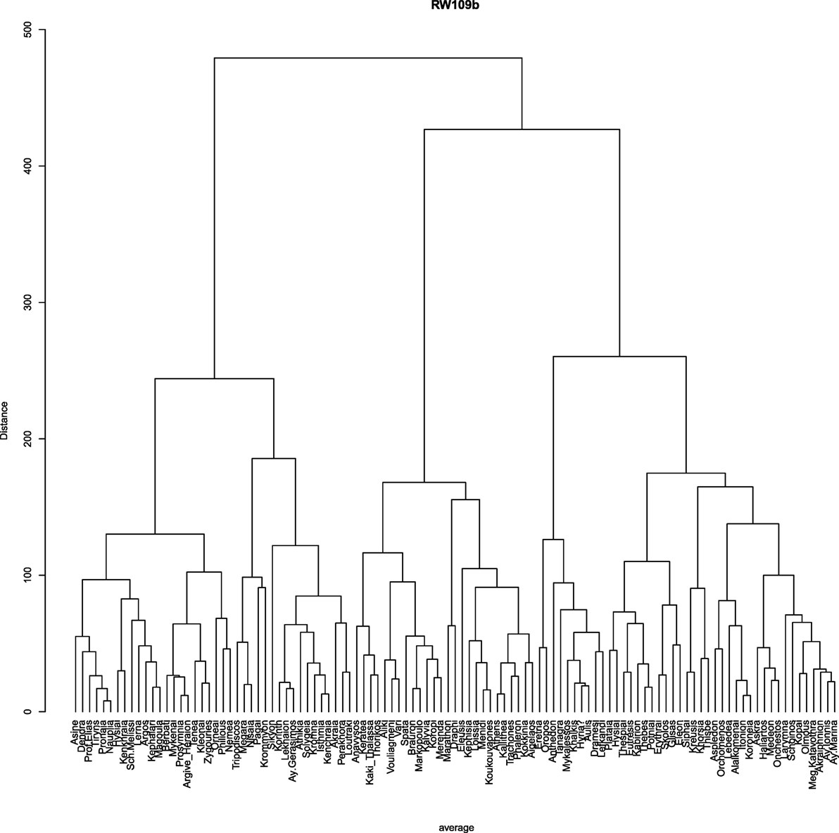
Figure 3. Hierarchical agglomerative clustering for the normal distance set using the average criterion for agglomeration.

3. The Rihll and Wilson Model

The model used by Rihll and Wilson (1987, 1991) and later authors (Wilson and Dearden, 2011; Bevan and Wilson, 2013; Rivers and Evans, 2014) to describe urbanization and state formation in historical contexts was originally devised to study the emergence of dominant retail centers (Huff, 1964; Lakshmanan and Hansen, 1965; Harris and Wilson, 1978). The model differs from several other well-known spatial models, such as Gravity Models, in that it is a “zone-of-control” model in the terminology of Evans et al. (2012). That is the model produces a structure of dominant sites, called “terminal sites,” surrounded by a cluster of smaller nearby satellite sites, see Figures 10 and 11.

In all that follows, we consider a network of N sites labeled i = 1, 2, …, N. As mentioned in Section 2.1, we take the sites to be equal, differing only in terms of their locations relative to one another. The output of the model will be a set of “flows” F_ij, each of which describes a flow from site i to a distinct site j, separated by an appropriately defined distance d_ij. In many spatial models, this flow F_ij represents the transmission of goods, people, influence, ideas, etc. from site i to site j. Here, however, we will use it to represent the “pulling power or attractiveness” (Rihll and Wilson, 1987, p. 8) of site i to site j. This is, of course, very abstract and unquantifiable, but in most ancient contexts, it is nearly always impossible to quantify exchanges of any type between sites, even where they are physical goods, so this is not a particular weakness of this study.

3.1. Construction of the Rihll and Wilson Model

In Appendix, we outline the derivation of the model through the maximum entropy approach of Wilson (1967). The key assumption is that if all other things are equal, then every possible exchange counted by the flows is equally likely. Of course in reality, there are strong constraints. We impose these here in three steps, producing first the simple gravity model, then the output constrained gravity model, and finally, the Rihll and Wilson model. We shall avoid algebra as much as possible here and refer the reader to Appendix, where it is given in a greater detail.

3.1.1. The Simple Gravity Model

Exchange between sites i and j requires some effort, and we imagine that this can be roughly quantified as a “cost” c_ij. For instance, the effort to maintain a link between two sites will generally increase with separation d_ij, so we might choose to capture this with the simple choice that our costs are equal to the distances, c_ij = d_ij. Our single constraint is that the total cost/effort that can be expended on exchange is capped. This is natural given that any society has limited resources. Making the best use of this knowledge (maximizing the entropy of the exchange flows subject to this constraint) gives the most likely distribution as

$F_{\mathit{ij}}=\mathit{Af}\left(d_{\mathit{ij}}/D\right),i\ne j.$ (1)

Here, the constant A is determined by the total cost we allow, but it can be fixed more easily by specifying the total amount of exchange, $F_{\text{total}}={\sum }_{i,j}{F}_{\mathit{ij}}$. The function f (x) is known as the deterrence function, and it expresses the effect of the costs incurred on a trip from i to j in terms of the distance. The likelihood of a single exchange occurring over distance d_ij is proportional to f (d_ij/D). The new parameter D is a calibration scale for the effect of distances on travel. Often f (x) is chosen such that f (0) = 1. The appropriate form for the deterrence function is rarely known, so another source of uncertainty comes from its choice. Note that we have swapped our lack of knowledge about the costs c_ij for the lack of knowledge about the function of distance f. Distances are more accessible quantities than costs, and we have some knowledge, or at least intuition, about the effect of distance on exchange. For instance, we imagine that the deterrence function should always decrease as distance gets larger, and indeed all our examples have this simple feature. Part of our study is to see how resilient the results from our modeling are to different choices.

A common form for the deterrence function corresponds to the simplest choice that costs are proportional to distances. This leads to the simple exponential form (labeled EXP in figures):

$f\left(d_{\mathit{ij}}/D\right)=\text{exp}\left(-d_{\mathit{ij}}/D\right).$ (2)

This is also the form used in the study by Rihll and Wilson (1987, 1991).

In general, the deterrence function can depend on additional calibration parameters that alter its shape, as we see in the second form shown in Figure 4. This ariadne deterrence function [or ariadne edge potential, labeled AEP in figures, and as used in the studies by Evans et al. (2006, 2012) and Knappett et al. (2008, 2011)] takes the form

$f\left(d_{\mathit{ij}}/D\right)={\left(1+{\left(d_{\mathit{ij}}/D\right)}^{\mathrm{\alpha }}\right)}^{-\mathrm{\gamma }}.$ (3)

FIGURE 4

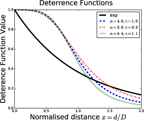
Figure 4. The exponential deterrence function (exp, solid line) of (2) and the ariadne deterrence function of [equation (3)] (dashed lines) in terms of x = d/D, the distance d scaled by the distance parameter D. The ariadne deterrence functions [equation (3)] shown for three of the nine parameter value combinations (α, γ) used in this work.

When compared to the exponential form [equation (2)], what we term the ariadne form [equation (3)] has low penalties for short-distance exchange but with a sharper change around distance scale D to a region where long-distance exchange is heavily penalized. For instance, we imagine that if D represents the typical distance traveled in a day overland in this region for our era, then it seems reasonable to impose a sharper difference between 1- and 2-day travel. This seems to us to be more appropriate for the case in hand, but translating qualitative expert judgments about the costs of exchange into a specific form for the deterrence function in our model is clearly another source of uncertainty. We can change of deterrence functions to try and evaluate how important this source of uncertainty is, and that is why we use two forms, the exponential form [equation (2)] and the ariadne form [equation (3)].

However, while the ariadne form [equation (3)] has the calibration distance scale D as one parameter, this form also has two further parameters, α and γ, which alter the shape of the function rather than the scale of the function. We will work with α = 3.6, 4.0, and 4.4 and while we will use γ values of 0.9, 1.0, and 1.1. We choose these particular shape parameter values because they represent a 10% variation around the standard choice made in our earlier work (Evans et al., 2006, 2012; Knappett et al., 2008, 2011). This ensures that the shape of these deterrence functions remains similar to our standard choice, little penalty for short-range exchange and heavy penalty for long-range exchange, but this allows us to probe uncertainty in the details of this particular modeling choice. We limit ourselves to just nine slightly different forms, so we can get a feel for the effect of this source of uncertainty in the deterrence function while keeping our study relatively simple. A full study of these additional parameters, and indeed of other deterrence function forms, is an avenue for future work, but even adding just two more parameters makes interpretation of outputs much harder.

3.1.2. The Output Constrained Gravity Model

The Simple Gravity model as given above can also be derived from a manifestly ontic, agent-based approach (Jensen-Butler, 1972). However, the Simple Gravity model is deficient in many ways.

One clear limitation is that there is no particular limit on the level of exchange emerging from each site in the Simple Gravity model; only the total amount of exchange is limited. By way of comparison, we note that some of the earliest and most successful examples of spatial modeling in archeology have employed Proximal Point analysis (for example, Terrell, 1977; Broodbank, 2000). Proximal Point analysis posits that each site only has interactions/exchanges with a fixed number of their closest sites, i.e., outflows are constrained. This has parallels in the idea that individuals only have the capacity to really interact with a limited number of other individuals (Dunbar, 1992).

Adding to the Simple Gravity model, the constraint that individual site outflows are fixed to be a given value O_i produces the Output Constrained Gravity model where the most likely exchange flows are found to be

$F_{\mathit{ij}}=A_i{O}_{i}f\left(d_{\mathit{ij}}/D\right),A_i^{-1}={\displaystyle \sum _j}f\left(d_{\mathit{ij}}/D\right),i\ne j.$ (4)

The normalization factors A_i ensure that the output from each site is indeed O_i, that is, $O_i={\sum }_j{F}_{\mathit{ij}}$.

3.1.3. The Rihll and Wilson Model

Unless we extend these models to accommodate strongly unequal site sizes initially, they have no mechanism for generating a handful of dominant sites as outputs, as identified in the archeological record. The presence of dominant sites requires the inclusion of non-linear behavior in the model constraints. Drawing on earlier work modeling retail outlets (Huff, 1964; Lakshmanan and Hansen, 1965; Harris and Wilson, 1978), Rihll and Wilson do this by constraining the entropy of the site inflows $I_j={\sum }_i{F}_{\mathit{ij}}$ although the motivation for this is best provided post hoc from the form of the final model. In the absence of this input entropy constraint, inflows over similar distance scales tend not to have wide variation as seen in either of the two previous models. The effect of this input entropy constraint is to give non-linear feedback so that sites that develop an advantage build on that advantage to become even more important, suggestive of the synoikism and urbanization that is expected to lie behind the appearance of regionally dominant sites. It is the inflow I_j outputs determined by the model that are used by Rihll and Wilson to assign an importance or “attractiveness” to a site.¹

The result (see Section B2 in Appendix) is that the flow F_ij from site i to site j (i ≠ j) now takes the form²

$F_{\mathit{ij}}=A_i{O}_i{I}_j^{\mathrm{\beta }}f\left(d_{\mathit{ij}}/D\right),A_i^{-1}={\displaystyle \sum _k}{I}_k^{\mathrm{\beta }}f\left(d_{\mathit{ij}}/D\right),i\ne j.$ (5)

As before, the normalization factors A_i ensure that the output from each site is indeed O_i. We stress that the total flows into each site j, the I_j, are not parameters of the theory but are all specified by the solution. The cost of each exchange is encoded in the deterrence function, f (d_ij/D), as before. Again, the model demands that the outputs are fixed. Given our limited information, we are unable to specify the outflows on a site-by-site basis, and we follow our usual response to a lack of information and take the outflows to be equal. Rihll and Wilson also set the output from each site to be equal as they suggest that it is most reasonable to assume that all sites were roughly equal in size and importance at the start of the period (see Rihll and Wilson, 1991, pp. 69–70).

The feature that distinguishes this model from other gravity models is the factor of $I_j^{\mathrm{\beta }}$ in equation (5). The $I_j^{\mathrm{\beta }}$ leads to solutions where for most sites I_j is zero or close to zero, so that all the available flow is input to a few sites, the “terminal sites,” which have significant input flows. These terminal sites send their output flows to a variety of other terminal sites. Roughly speaking, if the deterrence function becomes negligible for sites separated by distance scale D or more, then a site T with a large input flow (or attractiveness) I_T will suppress the attractiveness of sites within a radius of D or so through the normalization factor A_i. Basically a first guess is that in this model [equation (5)], the system will split up into patches of radius D, each with one dominant site. Indeed this is the typical pattern of solutions to the Rihll and Wilson model; a series of stars where all the flow leaving most sites is directed to just one site in their neighborhood, as can be seen in Figures 10 and 11.

3.2. Terminal Sites

The difference from gravity models with input and output constraints [for instance, see Evans et al. (2012)] is that outflows O_i are still input parameters of the theory, but now the inflows I_j are outputs determined by the model. These are used by Rihll and Wilson to assign an importance or “attractiveness” to a site.

To identify the most important sites, Rihll and Wilson use a particular implementation of a scheme of Nystuen and Dacey (1961), and we will follow suit. We define a terminal site to be a site where the total flow into that site is bigger than the largest flow out of that terminal site along any one edge. That is a terminal site T satisfies

$I_T={\displaystyle \sum _i}{F}_{\mathit{iT}}>F_{\mathit{Tj}}\forall j\ne T.$ (6)

Rihll and Wilson then compare the terminal sites found from the results of the model with the archeological record. In fact the nature of the output of the model, one dominated by obvious star like formations, which naturally define “zones of control,” means that we can pick these terminal sites out by eye from visualizations of the complete flow matrix in most cases, as in Figures 10 and 11.

4. Results

4.1. Assessing the Results

The basic idea in the original studies is to find the sites that emerge from the initial equal-sized settlements to dominate a region, based purely on the relative geographical positions.

In this context, there are certainly four cities that dominate the history of subsequent periods in this region: Thebes (25), Athens (70), Korinth (82), and Argos³ (101). We will use these four well-known sites as our key measure of the effectiveness of our various modeling attempts. Of course other sites play important roles; Rihll and Wilson provide commentaries on several other sites, both important and less so [throughout Rihll and Wilson (1987) and Rihll and Wilson (1991), but see p. 71 of the latter in particular]. Undoubtedly scholarship about the settlements in this region at this time will have moved on, but our focus is on the methodology and the role of uncertainty in modeling, so we are content to remain with a data set that captures the broad picture. It also enables us to build directly on the specific results present in the original articles.

Rihll and Wilson looked at several parameter values in their 1987 and 1991 papers for the exponential deterrence function of equation (2). Outcomes are determined by two parameters: the distance scale D of the deterrence function and the “attractiveness” exponent β. Their results for these four significant sites, as derived from their figures, are shown in Table 1. Thebes (25) and Athens (70) were always identified as terminal sites. Korinth (82) is identified in four of these figures, but sometimes the terminal site was not Korinth (82) itself but a close neighbor. There was also always a terminal at Argos (101) or a close neighbor.

TABLE 1

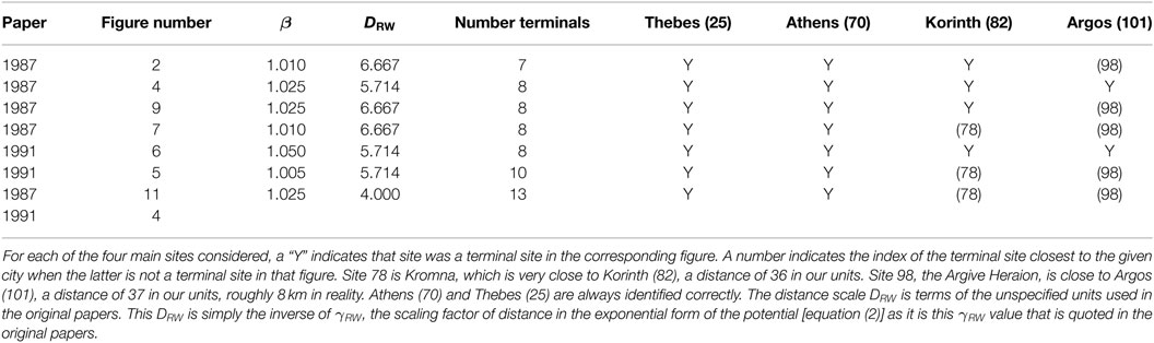
Table 1. The list of results for the seven different parameter values shown in the two Rihll and Wilson papers from 1987 and 1991.

In terms of robustness, Rihll and Wilson look at a range of parameter values, producing between eight and thirteen terminal in the Figures 4–6 of the study by Rihll and Wilson (1991). The key results are given in Table 1. We repeat this in the first stage of our study by looking at how sensitive our results are to changes in the calibration parameters D and β for a given deterrence function. In Figure 5, we show the sensitivity of the terminal number to the distance D and β parameter values, for the standard exponential deterrence function and for the normal (direct) distance set. This is broadly similar to Figure 6 of the study by Rihll and Wilson (1987). Essentially the only solutions that are relatively stable are those with three terminals. This is clear from the dendrograms of Figure 3 [see also equation (A7) in Appendix], where as the distance scale is raised, clusters start to form at around the minimum separation scale and then grow without any characteristics scale until they reach three clusters. There is then a long range of the distance scale where the dendrograms are stable with three clusters. Normally when clustering data, such a large region of stability is taken to indicate that this is a “good” clustering, and the user is confident that these clusters represent a significant feature in the data. Here, this stability with three clusters reflects the only clear spatial feature of our sites, the geographical gap that separates them into the three regions of Boeotia, Attica, and Isthmus/Argolid.

FIGURE 5

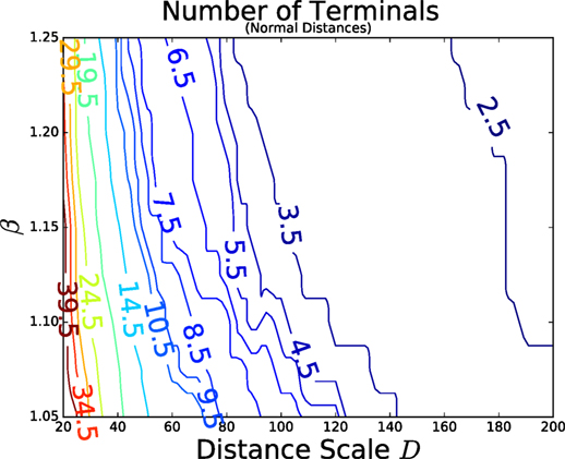
Figure 5. The number of terminal sites as the distance scale D and the non-linearity parameter β are varied. The contours are placed at half integer values as the actual terminal numbers are integers. For exponential potential [equation (2)] and normal distance set.

4.2. Fixed β

Both here and in the original articles, changing the non-linearity parameter β in the range 1.05–1.25 does not seem to change the qualitative nature of the results for choices of D; the pattern of terminals is qualitatively the same. So we will fix β, and then look at the remaining uncertainty in further detail. We chose to fix β = 1.05 as a typical value from the earlier studies. Initially we adopt the normal distance data set and the exponential deterrence function of equation (2) corresponding to the case where cost equals distance. The sensitivity to distance scale can be seen clearly for this fixed beta value in Figures 6 and 7.

FIGURE 6

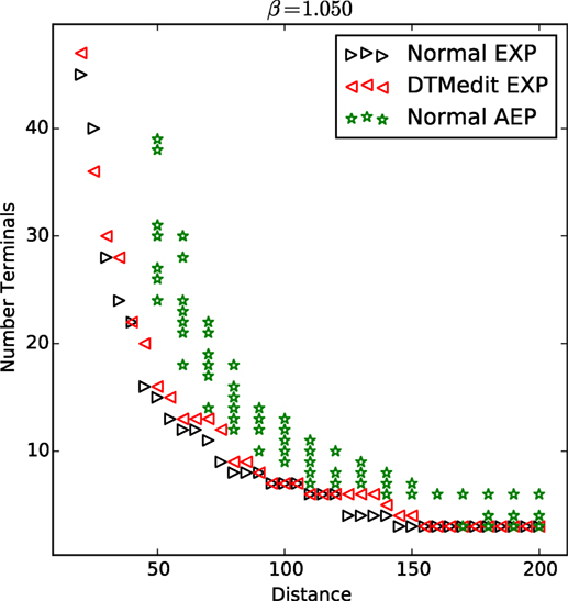
Figure 6. The number of terminal sites for various parameter values. The black triangles pointing right are for the normal distance set, while the red left pointing triangles are for the Delaunay Triangulation-derived distances, both using the exponential deterrence function. The green stars represent the normal distance used with the ariadne style deterrence function [equation (3)] using all nine possible combinations of α = 3.6, 4.0, or 4.4 along with γ = 0.9, 1.0, or 1.1. These are all for β = 1.05.

FIGURE 7

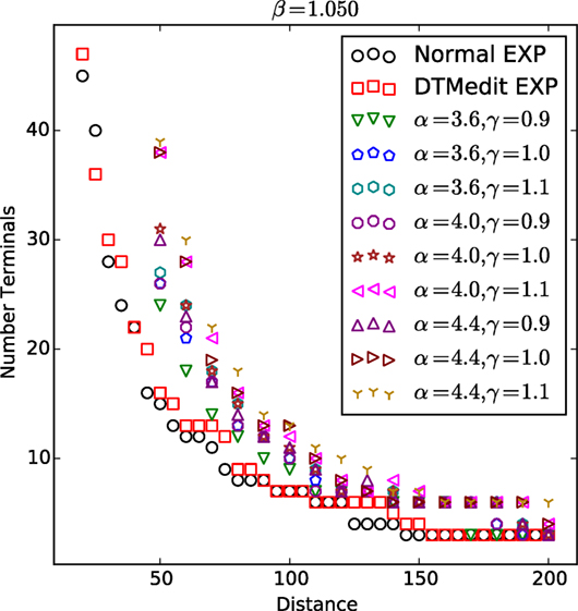
Figure 7. The number of terminal sites for various parameters. The black circles are for the normal distance set, while the red squares are for the Delaunay Triangulation-derived distances, both using the exponential deterrence function. These are generally below the other points, which are for the normal distance sets used with the ariadne style deterrence function (3) using all nine possible combinations of α = 3.6, 4.0, or 4.4 along with γ = 0.9, 1.0, or 1.1 as indicated by the legend. These are all for β = 1.05.

We have also repeated the analysis for our Delaunay Triangulation-based distances. The change of the distances from normal to Delaunay Triangulation-derived values has only a small effect. Generally, the latter reproduce the same number of terminals at a slightly higher distance scale. This is to be expected as the distances between any two points in the Delaunay-derived distances are always equal to or greater than the same points in the normal distance set. The main feature is that both these two cases using the exponential deterrence function show the instability in solutions with respect to small changes in the parameters as seen from the contour plots in Figure 5. So solutions with a given number of terminals T, when T is bigger than three, are only produced for very limited ranges of D, typically less 10 or less, roughly the nearest neighbor site separation.

As a separate exercise, Figures 6 and 7 illustrate the effects of changing the deterrence function to the ariadne form [equation (3)] with the values of its two further calibration parameters α and γ varied by 20%. We see the same instability as seen in the contour plots in terms of small changes in parameter D until we get to large distance scales with six or less terminal sites in their solution. Again the most stable solution has three terminals. The most interesting effect is that when we compare the solutions with the same number of T terminals and the same normal distance set, we see that changing the shape of the potential changes the value of the distance scale D.

This leads to an important conclusion. We should not try to compare two different theories at the same distance scale directly, even though in some qualitative way, they correspond to the mode of transport. The relationship between a parameter of a theory, here D, and the actual physical properties it corresponds to, perhaps the typical physical separation of our terminals, is highly non-trivial and depends on the details of the theory. This is a simple example of what is called “renormalization” in physics. What we must do is to pick a physical property, say the number of terminals, and then find the values of a theoretical parameter such as D where different models give similar physical results. Here, the exponential potential distances scales can be as little as half the ariadne deterrence function distance scales for results with the same number of terminals.

So for the next stage of investigation, we fix β and find solutions with a specified number T of terminal sites.

4.3. Eight Terminals

We choose to focus on model outputs with β = 1.05 and eight terminals, to see to what extent we can replicate Rihll and Wilson and how to take the analysis further. These are typical values considered in the original paper (Rihll and Wilson, 1991), with Figure 6 satisfying the criteria exactly. To do this, we start with our best representation of the distances between sites as outlines in Section 2.1. We set β = 1.05 and, initially, adopt the same exponential form for the deterrence function as shown in equation (2). We have to find our own distance scale D as the units used in the original papers are unknown. To do this, we scan through all possible value for D, other parameters fixed as described, looking for solutions with 8 terminals. We also repeated this exercise for the distances derived from our modified Delaunay Triangulation. The results are shown in Figure 8.

FIGURE 8

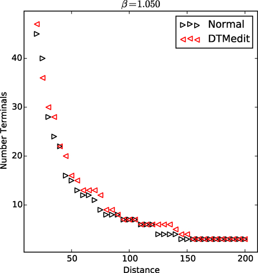
Figure 8. The number of terminal sites found using exponential deterrent function with β = 1.05. For normal (direct) distances and for distances based on modified Delaunay Triangulation (DTMedit).

We found three distinct solutions with eight terminals at D = 80, 85, and 90 for our normal distance matrix and only one at D = 90 for our modified Delaunay Triangulation (DTMedit) distance set. The precise sites are shown in Tables 2 and 3.

TABLE 2

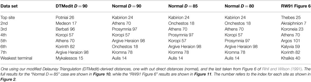
Table 2. The eight terminal sites found for β = 1.05 using an exponential deterrence function, ordered by the strength of the terminal flow.

TABLE 3

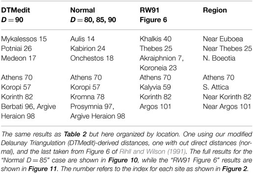
Table 3. The eight terminal sites found for β = 1.05 using an exponential deterrence function.

The results show a lot of consistency with variations on the scale of about 10 km. That is, all our examples give Athens (70) as one of the dominant sites, as Rihll and Wilson also found. There is also at least one terminal site close to Argos (101) and another close to Korinth (82), but often it is one of their close neighbors and not the sites that became dominant in later times. However, this is on a relatively small scale of roughly the average site separation, under 10 km. This “error” is emphasized by the fact none of our results here gives historic Thebes (25) as the dominant site, but rather we find one of its close neighbors. Looking at Table 2, we see the order of the sites, as defined by the terminal flow [see equation (A11) in Section B1 of Appendix], moves around between the different solutions on top of the actual again emphasizing the level of robustness of the results.

Perhaps more interestingly, Table 3 shows a clear difference between the three distance sets, the original (unknown) Rihll and Wilson distances, our normal direct distances, and the modified Delaunay Triangulation (DTMedit)-derived distances. Apart from Athens (70), the dominant site in each region is different in at least two and mostly in all three cases. So we see that different choices of distance measures do have an effect. On the other hand, the changes are small, on this nearest neighbor scale of a few kilometers. Uncertainty on this scale is to be expected given the uncertainty of other aspects of the modeling. It is almost certainly also no worse than the uncertainty coming from our lack of detailed knowledge of the actual terrain (geographical, political, and social) of the period.

4.4. Three Terminals

The clustering suggests that three terminal solutions are the only ones, which are in a noticeably stable region of parameter space. We are not suggesting that, in this period, there were only three significant sites. Our purpose is to understand the nature of the modeling process better when there is less ambiguity. The three sites found for the exponential deterrence function and the two different distance sets are given in Table 4. As might be expected given the noticeable gap visible to the eye in the map of sites in Figure 2, there is one site for each of the three clear regions: Boeotia, Attica, and Isthmus/Argolid.

TABLE 4

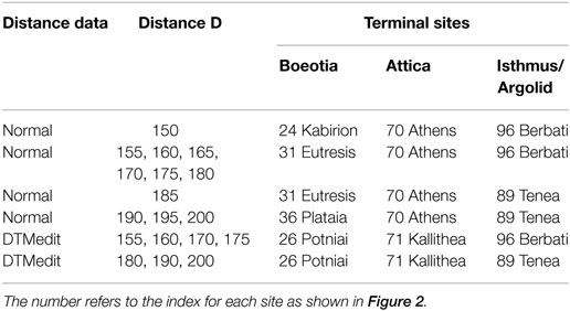
Table 4. The three terminal sites for normal and Delaunay Triangulation distance data with the exponential deterrence function when solutions have exactly three terminals.

For Boeotia, yet again Thebes (25) itself is never a terminal, but the terminal site picked is always close to Thebes (25). Unlike the results for eight terminals, this site is no longer always a nearest neighbor, e.g., Plataia (36) is about 13 km south of Thebes (25).

For Attica, we find that the Delaunay Triangulation distance data no longer pick Athens (70) but instead pick an extremely close neighbor of Athens (70). The difference between the two data sets reflects the fact that they differ only on longer distance scales. With three terminals, each site is the center of attraction for about a third of the sites spread over a much larger distance, so the differences between the two distance sets will be more important when we have fewer terminals.

The most interesting case is the terminal in the Isthmus/Argolid region, either Berbati (96) or Tenea (89) being chosen. These sites are somewhere in between the two neighborhoods, that close to Argos (101) and the second around Korinth (82), which provided Ishmus/Argolid region terminal sites when there were eight terminals in total. What this result suggests is that to a first approximation, the Rihll and Wilson model splits the space into roughly equal area patches and with one terminal per region, the terminal lying close to the geometric center of its region.

This has implications for our more general analysis, which we now test.

4.5. The Cluster-and-Center Method

The typical type of network produced by the Rihll and Wilson model is shown in Figure 11. It shows a set of connected stars, zones of influence, where the terminal sites are each the center of one star, while remaining other sites only have one strong connection to a nearby terminal site. This effectively defines a clustering of the sites⁴ where each cluster contains one terminal site along with all the sites with a strong connection to the terminal site of the cluster. Looking at the solutions, it appears that the terminals are often close to the geometric center of the clusters. This is not surprising as the site closest to the center is likely to minimize the sum over deterrence function terms in the denominator of equation (5), which would allow a larger I_i value in the solutions, and large I_j values characterize the terminal sites.

This leads us to the conjecture that the Rihll and Wilson model is clustering close sites and then giving the most central node as the terminal node. One way to test this is to attempt a different approach to finding the key sites, which we will refer to as a “cluster-and-center” method. This is a null phenomenological approach, relying on geographic data alone, without the trappings of entropy and Bayesian analysis. First, we use a standard data clustering method, one which takes distances between data points (here the sites) as their input. The only parameter of the method is the number of clusters to be considered. Once we obtain our clusters of sites, we then find the most central site by looking for the site, which is closest to the point with coordinates given by the mean (or the median) of the coordinates of all the sites in the cluster.

In Table A2 in Appendix, we show the results for eight clusters, so that we can compare them with the eight terminal results discussed above. We used k-means clustering and five variations of hierarchical agglomerative clustering (HAC) [for example, see Manning et al. (2008), for both methods]. The implementation of k-means clustering that we use is stochastic so we are just showing one possible result here.

For three of the four flagship sites, we are using to test results; this approach gives reasonable results, except when using the method labeled “HAC single.” The “single” version of hierarchical agglomerative clustering is well known to be an extreme version and is often not appropriate. It is clearly an outlier here, and we will ignore it from now on.⁵ For the remaining five methods shown in Table A2 in Appendix, Argos (101) is always picked as a center. Korinth (82) is only picked out only once, and either Lekhaion (80, 3 km north of Korinth) or Kromna (78, 6 km East of Korinth) are chosen instead. However, these are close neighbors of Korinth (82), and so we are finding the methods choose the same type of 10 km wide region as we did with the Rihll and Wilson model. Athens (70) is picked out most often in the northern Attica region (six times from the ten reasonable methods) with Koropi (57, 12 km north of Athens) or Menidi (50, 15 km south east of Athens) picked otherwise. However, neither of these alternative sites is particularly close to Athens (70), lying outside the range of results we found with the Rihll and Wilson model.

The big difference comes in the Boeotian region. Thebes (25) is never picked out. Further, the two close neighbors in the typical small region picked out in our analysis using the Rihll and Wilson model, Potniai (26, 3 km south of Thebes) and Kabirion (24, 7 km west of Thebes), are only picked out in only four of the ten reasonable results.

Overall, while there is some correlation between the Rihll and Wilson model and the cluster-and-Center method outlined in this section, it is not an overwhelmingly strong or clear relationship. We need more than geography to understand why some sites develop to become so important at the expense of their neighbors. The entropic/Bayesian approach of Rihll and Wilson provides a useful next step to our understanding of state formation.

5. Conclusion

In our earlier paper (Rivers and Evans, 2014), we speculated on the contingent nature of Thebes in the Rihll and Wilson model, taking their results for granted. In this article, we have shown that Thebes (or, indeed, any site) can only be understood in the much larger context of uncertainty in spatial network modeling and how this is reflected in model outcomes, a context which has implications for all entropic attempts to understand urbanization and city-state development.

We have highlighted several sources of uncertainty: site choice, distances, model choice, parameter choice. In this article, we have looked at the effect on outcomes of some (but not all) of these sources of uncertainty. We have tried two ways to calculate distances, our normal and Delaunay Triangulation-derived distances. By comparing with the results of the study by Rihll and Wilson (1987, 1991), we have effectively a third set of distances—those used by Rihll and Wilson. We have tried also two major ways to encode the costs of distance in the models: an exponential deterrence function [equation (2)] and the ariadne deterrence function [equation (3)].

An important requirement of this work is that to evaluate uncertainties we must make fair comparisons between results from different variations of the same model or even completely different models. The key problem is that we do not know what parameter values to use in different models to make this fair comparison. Even when a parameter is apparently linked to a physically measurable scale, such as our distance scale parameter D, the relationship between model value and actual measurable physical quantity is complicated. Should we relate the distance scale D directly to the typical daily walking distance, or should that be 1.5D or 0.9D? Whatever this relationship is, it will change with different model parameter values and indeed when using different models. This is the key principle of “renormalization,” which we must never assume that a model parameter is simply related to a physical quantity. The answer we suggest is to compare results from different models only when they are giving the same output by some suitable measure.

In terms of the data used in this article, we have arrived at similar conclusions to the original authors, although we put these within larger but quantified margins of uncertainty. Our results show that there are regions about 10 km across, which have distinct geographical advantages for encouraging urbanization and which can help explain the different roles of sites in later periods. We do not predict that Thebes, and to a lesser extent Athens, are always going to be these sites, unlike the original papers, but we do agree that sites in their close neighborhood are continually shown to have this advantage. Thebes is not necessary, but something like it was always likely.

Of course similar links have been made between geographical locations and the role of sites in history: Delos in the case of Davis (1982) and Knossos in the case of Knappett et al. (2008). However, in the latter case, the modeling also suggested that a pair of candidates, Knossos and Malia, had these spatial advantages, again compatible with the uncertainties in modeling.

In terms of the method of Rihll and Wilson itself, our work has highlighted that, qualitatively at least, it seems to divide up the sites into regions of roughly equal size, each with a terminal site. To test the hypothesis that the terminals are close to the geometric centers of these zones, we have compared this “zone-of-control” spatial ordering against a null “cluster-and-center” method, which is based on generic clustering methods using geographical data alone. Specifically, it takes any clustering method to create the clusters and then finds their geometric centers to locate the dominant site for each cluster. This enables us to come up put “error bars” on our results, estimates of the range of reasonable results as illustrated in Figure 9.

FIGURE 9

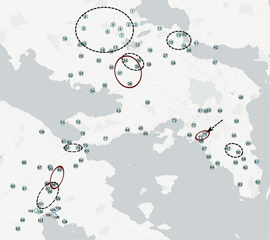
Figure 9. Ranges of uncertainty for the terminal sites. The black dashed ellipses and the arrow indicate the range of possible locations for the eight terminal solutions of Section 4.3. The red solid ellipses show where we find terminal sites when there are only three in total in any one solution as discussed in Section 4.4.

FIGURE 10

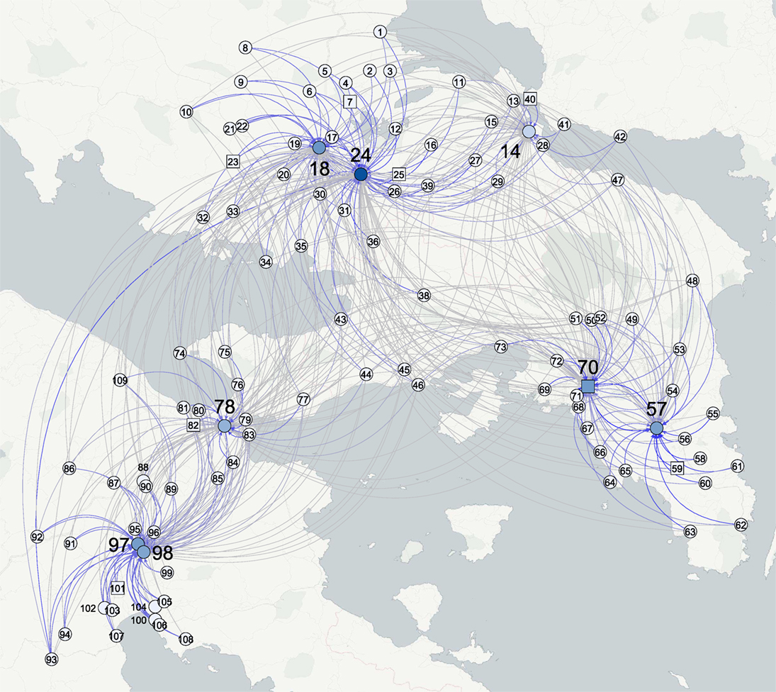
Figure 10. A solution for the Rihll and Wilson model (5) with an exponential deterrent function, D = 85, β = 1.05 using normal (direct) distances. The darker the color of an edge, the large the flow along that edge. The larger and darker the symbol used for each site, the larger the flow into that site. This produces eight terminal sites: 14 Aulis, 18 Onchestros, 24 Kabirion, 57 Koropi, 70 Athens, 78 Kromna, 97 Prosymnia, and 98 Argive Heraion. The square sites are the eight terminal sites shown in Figure 6 of Rihll and Wilson (1991): 7 Akraiphnion, 23 Koroneia, 40 Khalkis, 25 Thebes, 59 Kalyvia, 70 Athens, 82 Korinth, and 101 Argos.

FIGURE 11

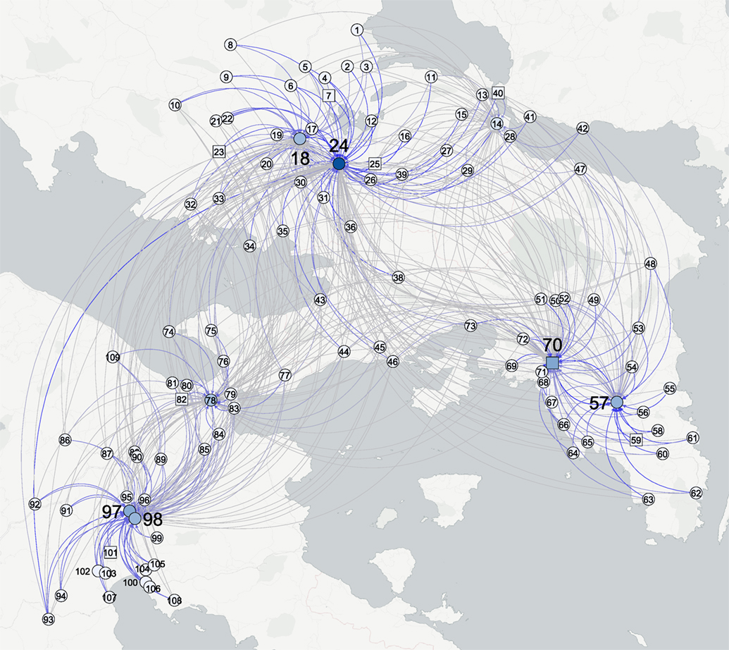
Figure 11. A solution for the Rihll and Wilson model (5) with an exponential deterrent function, D = 90, β = 1.05 using normal (direct) distances. The darker the color of an edge, the large the flow along that edge.

For the clustering methods we tried here, we found there is some correlation between the Rihll and Wilson model and the cluster-and-Center method. However, it is not an overwhelmingly strong or clear relationship. It seems that we need more than geography alone, a need arguably satisfied in part by entropic/Bayesian analysis. It could be argued that the popular and generic data clustering methods we used here, k-means and hierarchical agglomerative clustering, are more effective on higher dimensional data than our two-dimensional world surface. However, even if it had been in better agreement with our outputs, which we do not think is likely, part of the rationale for using the Rihll and Wilson model is the interpretation it brings. The Rihll and Wilson model comes with a powerful epistemic interpretation in terms of the entropy of microstates and a natural interpretation in terms of flows, inputs, outputs, and costs. We learn from the nature of the calibration. A regular data clustering method such as k-means brings no intrinsic interpretation to the table, and it merely hopes to provide reasonable clusterings in a calibration-free way.

The archeological context has been the Argos–Korinth– Athens–Thebes region of Greece in the Late Geometric era. This context was chosen so that we can illustrate general methodological principles with a practical archeological example, with the added benefit that it allows us to make direct contact with the classic work of Rihll and Wilson (1987, 1991). The last decade has seen a rise in the use of such modeling techniques on settlement patterns in a wide range of times and other places: Crete in the second millennium BC (Bevan and Wilson, 2013) or the Middle Bronze Age (Evans et al., 2006; Knappett et al., 2008, 2011; Paliou and Bevan, 2016), Iron Age NE Syria (Davies et al., 2014), early second millennium BC Central Anatolia (Palmisano and Altaweel, 2015), late first Millennium Latenian urbanization (Filet, 2017), early Japan (Mizoguchi, 2009), the Maya lowlands (Ducke and Kroefges, 2008), to give just a few examples. Similar methods can be used when modeling of other types of spatial organization, such as lithic assemblages (Wilson, 2007) to name just one. The range of applications of such modeling now appearing suggests that this approach is mature enough that we should look to include uncertainty as an intrinsic part of such work. Our view echoes that of other authors who tackle other aspects of the uncertainty problem (e.g., Bevan and Wilson, 2013; Davies et al., 2014; Paliou and Bevan, 2016). Using these emerging approaches to account for uncertainty will only enhance the contribution modeling can make to our overall picture of the past.

Author Contributions

This paper is based on a talk given by RR at EAA, Glasgow 2015 and by TE at Univ. Konstanz 20th September 2016 (Evans, 2016b). TE wrote the computer codes and prepared the data and maintains a freely available archive of the data, see Evans (2016a). Both TE and RR contributed to all other aspects of the work.

Conflict of Interest Statement

The authors declare that the research was conducted in the absence of any commercial or financial relationships that could be construed as a potential conflict of interest.

Acknowledgments

RR thanks the organizers of the session at EAA Glasgow where this work was presented. RR and TE also thank Ulrik Brandes and the Konstanz group for discussions during the workshop on Archaeological Network Reconstruction.

Footnotes

1. ^In a second self-consistent version, Rihll and Wilson set the outputs equal to the inputs in a self-consistent manner O_i = I_i, so the number of arrivals is the number of departures. The model parameters then include an initial value for I_i for each site. We will not consider this self-consistent variant further.
2. ^Note that it is standard to ignore the internal flows, the entries F_ii. Equivalently we choose f, so that f(d_ii/D) = f(0)=0.
3. ^To this list Rihll and Wilson add a fifth site, Khalkis (40) (see Rihll and Wilson, 1991, p. 71), which is about 30 km north east of Thebes at the narrowest point between the mainland and the large island of Euboea. Khalkis was significant enough to found several other Greek cities.
4. ^This is called a community of sites in network science, and, more formally, this is a partition of the set of sites.
5. ^Further discussion and more detailed results supporting this are given in the Appendix, Section C.

References

Alonso, W. (1978). “A theory of movements,” In Human Settlement Systems: International Perspectives on Structure, Change and Public Policy, Edited by N. M. Hansen, 197–211. Cambridge, MA: Ballinger.

Google Scholar

Altaweel, M. (2015). Settlement dynamics and hierarchy from agent decision-making: a method derived from entropy maximization. Journal of Archaeological Method and Theory 22: 1122–50. doi:10.1007/s10816-014-9219-6

CrossRef Full Text | Google Scholar

Babtie, A.C., Kirk, P., and Stumpf, M.P. (2014). Topological sensitivity analysis for systems biology. Proceedings of the National Academy of Sciences of the United States of America 111: 18507–12. doi:10.1073/pnas.1414026112

PubMed Abstract | CrossRef Full Text | Google Scholar

Bevan, A., and Wilson, A. (2013). Models of settlement hierarchy based on partial evidence. Journal of Archaeological Science 40: 2415–27. doi:10.1016/j.jas.2012.12.025

CrossRef Full Text | Google Scholar

Broodbank, C. (2000). An Island Archaeology of the Early Cyclades. Cambridge: Cambridge University Press.

Google Scholar

Coldstream, J.N. (2003). Geometric Greece: 900-700 BC. London: Routledge.

Google Scholar

Davies, T., Fry, H., Wilson, A., Palmisano, A., Altaweel, M., and Radner, K. (2014). Application of an entropy maximizing and dynamics model for understanding settlement structure: the Khabur Triangle in the Middle Bronze and Iron Ages. Journal of Archaeological Science 43: 141–54. doi:10.1016/j.jas.2013.12.014

CrossRef Full Text | Google Scholar

Davis, J. (1982). Thoughts on prehistoric and archaic Delos. Temple University Aegean Symposium 7: 23–23.

Google Scholar

Ducke, B., and Kroefges, P.C. (2008). From points to areas: constructing territories from archaeological site patterns using an enhanced xtent model. In Layers of Perception. Proceedings of the 35th International Conference on Computer Applications and Quantitative Methods in Archaeology (CAA), Berlin, April 2–6, 2007, Kolloquien zur Vor- und Frühgeschichte, Vol. 10, Edited by A. Posluschny, K. Lambers, and I. Herzog, 245–251. Bonn: Dr. Rudolf Habelt GmbH.

Google Scholar

Dunbar, R. (1992). Neocortex size as a constraint on group size in primates. Journal of Human Evolution 22: 469–93. doi:10.1016/0047-2484(92)90081-J

CrossRef Full Text | Google Scholar

Evans, T., Knappett, C., and Rivers, R. (2006). Physical and relational networks in the Aegean Bronze Age. In Proceedings of the European Conference on Complex Systems, Edited by J. Jost, F. Reed-Tsochas, and P. Schuster, 81. ECCS. doi:10.6084/m9.figshare.750447

CrossRef Full Text | Google Scholar

Evans, T., Rivers, R., and Knappett, C. (2012). Interactions in space for archaeological models. Advances in Complex Systems 15: 1150009. doi:10.1142/S021952591100327X

CrossRef Full Text | Google Scholar

Evans, T.S. (2016a). Locations of 109 Archaic Greek Settlements Used in Rihll and Wilson 1987. Springer/Nature. doi:10.6084/m9.figshare.868961

CrossRef Full Text | Google Scholar

Evans, T.S. (2016b). Uncertainty and Spatial Models: The Effects of Space on Network Analysis. figshare. doi:10.6084/m9.figshare.3840249.v1

CrossRef Full Text | Google Scholar

Filet, C. (2017). An attempt to estimate the impact of the spread of economic flows on latenian urbanisation. Frontiers in Digital Humanities 3: 10. doi:10.3389/fdigh.2016.00010

CrossRef Full Text | Google Scholar

Harris, B., and Wilson, A. (1978). Equilibrium values and dynamics of attractiveness terms in production-constrained spatial-interaction models. Environment and Planning A 10: 371–88. doi:10.1068/a100371

CrossRef Full Text | Google Scholar

Huff, D.L. (1964). Defining and estimating a trading area. Journal of Marketing 28: 34–8. doi:10.2307/1249154

CrossRef Full Text | Google Scholar

Jaynes, E.T. (1957). Information theory and statistical mechanics. Physical Review 106: 620. doi:10.1103/PhysRev.106.620

CrossRef Full Text | Google Scholar

Jaynes, E.T. (1973). The well-posed problem. Foundations of Physics 3: 477–92. doi:10.1007/BF00709116

CrossRef Full Text | Google Scholar

Jensen-Butler, C. (1972). Gravity models as planning tools: a review of theoretical and operational problems. Geografiska Annaler Series B Human Geography 54: 68–78. doi:10.2307/490586

CrossRef Full Text | Google Scholar

Kennedy, M., and O’Hagan, A. (2001). Bayesian calibration of computer models. Journal of the Royal Statistical Society Series B (Statistical Methodology) 63: 425–64. doi:10.1111/1467-9868.00294

CrossRef Full Text | Google Scholar

Keynes, J.M. (1921). A Treatise on Probability. London: MacMillan.

Google Scholar

Knappett, C., Evans, T., and Rivers, R. (2008). Modelling maritime interaction in the Aegean Bronze Age. Antiquity 82: 1009–24. doi:10.1017/S0003598X0009774X

CrossRef Full Text | Google Scholar

Knappett, C., Evans, T., and Rivers, R. (2011). The Theran eruption and Minoan palatial collapse: new interpretations gained from modelling the maritime network. Antiquity 85: 1008–23. doi:10.1017/S0003598X00068459

CrossRef Full Text | Google Scholar

Lakshmanan, J., and Hansen, W.G. (1965). A retail market potential model. Journal of the American Institute of Planners 31: 134–43. doi:10.1080/01944366508978155

CrossRef Full Text | Google Scholar

Laplace, P.-S. (1825). Essai philosophique sur les probabilités. Paris: Bachelier.

Google Scholar

Manning, C.D., Raghavan, P., and Schütze, H. (2008). Introduction to Information Retrieval. Cambridge: Cambridge University Press.

Google Scholar

Mizoguchi, K. (2009). Nodes and edges: a network approach to hierarchisation and state formation in Japan. Journal of Anthropological Archaeology 28: 14–26. doi:10.1016/j.jaa.2008.12.001

CrossRef Full Text | Google Scholar

Neapolitan, R.E., and Jiang, X. (2014). A note of caution on maximizing entropy. Entropy 16: 4004–14. doi:10.3390/e16074004

CrossRef Full Text | Google Scholar

Nystuen, J.D., and Dacey, M.F. (1961). A graph theory interpretation of nodal regions. Papers of the Regional Science Association 7: 29–42. doi:10.1007/bf01969070

CrossRef Full Text | Google Scholar

Paliou, E., and Bevan, A. (2016). Evolving settlement patterns, spatial interaction and the socio-political organisation of late prepalatial south-central crete. Journal of Anthropological Archaeology 42: 184–97. doi:10.1016/j.jaa.2016.04.006

CrossRef Full Text | Google Scholar

Palmisano, A., and Altaweel, M. (2015). “Simulating past human landscapes: models of settlement hierarchy in Central Anatolia during the Old Assyrian Colony period,” In Proceedings of the 1st Kültepe International Meeting, Kültepe, September 19–23, 2013. Studies Dedicated to Kutlu Emre. Kültepe International Meetings 1 (SUBART 35), Edited by F. Kulakoğlu and C. Michél, 131–146. Brepols: Turnhout.

Google Scholar

Rihll, T., and Wilson, A. (1991). Modelling settlement structures in ancient Greece: new approaches to the polis. In City and Country in the Ancient World, Vol. 3, Edited by J. Rich and A. Wallace-Hadrill, 58–95. London: Routledge.

Google Scholar

Rihll, T.E., and Wilson, A.G. (1987). Spatial interaction and structural models in historical analysis: some possibilities and an example. Histoire & Mesure 2: 5–32. doi:10.3406/hism.1987.1300

CrossRef Full Text | Google Scholar

Rivers, R., and Evans, T. (2014). New approaches to Archaic Greek settlement structure. Les Nouvelles de l’archéologie 135: 21–7. doi:10.4000/nda.2316

CrossRef Full Text | Google Scholar

Terrell, J. (1977). Human biogeography in the Solomon Islands. Fieldiana Anthropology 68: 1.

Google Scholar

Wilson, A. (1967). Statistical theory of spatial distribution models. Transport Research 1: 253. doi:10.1016/0041-1647(67)90035-4

CrossRef Full Text | Google Scholar

Wilson, A. (2008). Boltzmann, Lotka and Volterra and spatial structural evolution: an integrated methodology for some dynamical systems. Journal of the Royal Society Interface 5: 865–71. doi:10.1098/rsif.2007.1288

PubMed Abstract | CrossRef Full Text | Google Scholar

Wilson, A., and Dearden, J. (2011). Phase transitions and path dependence in urban evolution. Journal of Geographical Systems 13: 1–16. doi:10.1007/s10109-010-0134-4

CrossRef Full Text | Google Scholar

Wilson, L. (2007). Understanding prehistoric lithic raw material selection: application of a gravity model. Journal of Archaeological Method and Theory 14: 388–411. doi:10.1007/s10816-007-9042-4

CrossRef Full Text | Google Scholar

Appendix

A. Index of Sites

A list of sites giving their index and name is in Table A1 in Appendix. The positions are found from the locations of a digitized version of Figure 1 in the study by Rihll and Wilson (1987) with site coordinates given in our units. For instance, in our “normal” distance set, which uses the direct distance between sites, we have that site 1, Laryma, and site 109, Sikyon are separated by a distance is $\sqrt{{\left(469.5-190.5\right)}^2+{\left(169.1-536.2\right)}^2}\approx 461\text{\hspace{0.17em}U}$. The actual straight line distance is about 82 km, and so the distance scale used in this paper is roughly 6 U for 1 km.

TABLE A1

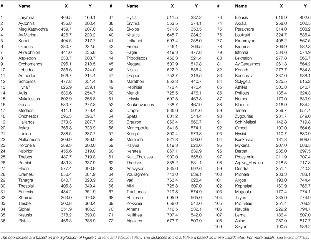
Table A1. Index of 109 sites used here.

B. Technical Details of the Rihll and Wilson Gravity Model

The model used in the work of Rihll and Wilson (1987, 1991) was originally devised to determine the best position of retail centers (Huff, 1964; Lakshmanan and Hansen, 1965; Harris and Wilson, 1978) [see p. 11 of Rihll and Wilson (1987) for further citations].

Consider a network of N sites labeled i = 1, 2, …, N. The model produces the link strengths F_ij, which describe the flows from sites i to sites j. As a result, the total outflow from the site i is $O_i={\sum }_j{F}_{\mathit{ij}}$ and the total incoming flow to site j ps $I_j={\sum }_k{F}_{\mathit{kj}}$. Here, we will outline the derivation of the model using an entropy viewpoint pioneered by Wilson in the context of generic spatial modeling (Wilson, 1967). The key assumption is that if all other things are equal, then every possible exchange counted by the flows is equally likely. Put another way, if there is no other information about these exchanges, then the best we can do is to assume all exchanges are equally likely. The maximum entropy framework provides a rigorous mathematical basis for this simple idea.

Of course in reality, there are strong constraints and different models add in different types of extra information in an attempt to provide a more realistic description of the individual exchanges. Equivalently, they can be understood as the most likely configurations of a microcanonical ensemble subject to these same constraints.

For the shopping model (Huff, 1964; Lakshmanan and Hansen, 1965; Harris and Wilson, 1978) used by Rihll and Wilson, the flows defined by the model maximize the entropy S, more conveniently understood as minimizing the Hamiltonian H = − S, where, after some rewriting (Harris and Wilson, 1978), Equations (30)–(33).

$\begin{array}{l}H={\displaystyle \sum _{i,j}}{F}_{\mathit{ij}}\left(\text{ln}\left(F_{\mathit{ij}}\right)-1\right)-{\displaystyle \sum _i}{\mathrm{\alpha }}_i\left[O_i-{\displaystyle \sum _j}{F}_{\mathit{ij}}\right]\\ -\mathrm{\beta }\left[C-{\displaystyle \sum _{i,j}}\left(F_{\mathit{ij}}{c}_{\mathit{ij}}\right)\right]+\mathrm{\beta }\left[X-{\displaystyle \sum _j}{I}_j\left(\text{ln\hspace{0.17em}}{I}_j-1\right)\right].\end{array}$ (A1)

The solutions are the most likely pattern for exchanges given the constraints [given in the square brackets in equation (A1)] imposed in the model. For simplicity, we are assuming that every site i has the same number of potential origins or destinations for a trip. The first term reflects the assumption that the probability that an exchange occurs on any given edge is independent of the edge if all other things are equal. The second term, with coefficient α imposes a constraint that the total output of site i, the total flow leaving site i, is equal to a parameter O_i, which we must specify. The third term supposes that the cost of each exchange from i to j is c_ij and that we demand that the total cost is C, another parameter we must satisfy. This “cost” is not necessarily in terms of money. Rather it is generally expressed in terms of some characteristic fixed by the geography of the site, typically some measure of the distance between two sites. All of the first three terms are frequently seen in this type of entropy approach. It is the last term, which is distinctive and is a key feature of the model of Rihll and Wilson. It involves the total incoming flow, $I_j={\sum }_k{F}_{\mathit{kj}}$, but it is not a simple constraint on the total input to each site.

Rather, it is a constraint on the entropy of site outflows that, in the absence of this (and other constraints), would be uniform. To understand what type of effect this last term is giving, and indeed to get a better understanding of what all the terms lead to, it is easier to quote the solution for the pattern of flows, which maximizes the entropy, which can be expressed in a simple algebraic form as

$F_{\mathit{ij}}=A_i{O}_i{I}_j^{\mathrm{\beta }}{f}_{\mathit{ij}},A_i^{-1}={\displaystyle \sum _k}{I}_k^{\mathrm{\beta }}{f}_{\mathit{ik}}{I}_j={\displaystyle \sum _i}{f}_{\mathit{ij}}.$ (A2)

The parameters α_i have been fixed by the requirement that the outputs for each site are fixed to be are O_i from, which the normalization factors A_i are determined in terms of other quantities in the theory. The total cost C and the cost of each exchange c_ij are equivalent to specifying what is known as the deterrence function f_ij,

$f_{\mathit{ij}}=\text{exp}\left(-c_{\mathit{ij}}/D\right),$ (A3)

where D is a distance scale against which “costs” are measured. More generally, we write

$f_{\mathit{ij}}=f\left(d_{\mathit{ij}}/D\right),$ (A4)

where f (x) relates costs to the separation variables d_ij between sites i and j. For instance, if the costs are just the distances, c_ij = d_ij, then we arrive at a simple exponential form

$f_{\mathit{ij}}=\text{exp}\left(-d_{\mathit{ij}}/D\right).$ (A5)

We stress that the outflows O_i are input parameters for the Rihll and Wilson model [equation (A2)], whereas the inflows $I_j={\sum }_i{F}_{\mathit{ij}}$ are to be determined from equation (A2) as outputs from the model. The inflows are interpreted as the attractiveness or importance of a site and as used to determine the dominant city-state sites.

In this case, varying site size can be accommodated. The obvious extension to include site size [that has its counterpart in the work of Alonso (1978)] is to take

$\begin{array}{l}H={\displaystyle \sum _{\left(i,j\right)}}{F}_{\mathit{ij}}\left[\text{ln}\left(\frac{F_{\mathit{ij}}}{S_i{S}_j}\right)\right]-{\displaystyle \sum _i}{\mathrm{\alpha }}_i\left[O_i-{\displaystyle \sum _j}{F}_{\mathit{ij}}\right]\hfill \\ -\mathrm{\beta }\left[C-{\displaystyle \sum _{i,j}}\left(F_{\mathit{ij}}{c}_{\mathit{ij}}\right)\right]-\mathrm{\beta }\left[X-{\displaystyle \sum _j}{I}_j\left(\text{ln}\left(\frac{I_j}{S_j}\right)-1\right)\right].\hfill \end{array}$ (A6)

Extremal solutions now take the form

$F_{\mathit{ij}}=S_i{S}_j^{1-\mathrm{\beta }}{e}^{-{\mathrm{\alpha }}_i}{I}_j^{\mathrm{\beta }}{f}_{\mathit{ij}}.$ (A7)

Consistency then requires that

$F_{\mathit{ij}}=A_i{O}_i{S}_i^{1-\mathrm{\beta }}{I}_j^{\mathrm{\beta }}{f}_{\mathit{ij}},A_i^{-1}={\displaystyle \sum _k}{S}_j^{1-\mathrm{\beta }}{I}_k^{\mathrm{\beta }}{f}_{\mathit{ik}}.$ (A8)

We said that, in the absence of further evidence, we had taken all the S_i to be identical. We note that explicit dependence on site size is very weak, going as $S_i^{1-\mathrm{\beta }}$, where 1 − β ≈ 0.05, with negligible effect. However, there is implicit dependence in the way the given outputs depend on site size (e.g., O_i ∝ S_i).

B.1. Non-Linearity in the Rihll and Wilson Model

The factor of $I_j^{\mathrm{\beta }}$ in the Rihll and Wilson model is the key difference from most other gravity models. This term introduces non-linear feedback based on the inputs through the self-consistent normalization factors.

To understand how this works, we will consider a simple way to find the solution to equation (A2) for a given set of parameters. The idea is that if we are given a set of input flows at some time t, say I_j(t), then we specify the next round of values at iteration number (t + 1), I_j(t + 1). To show this iterative process, we first rewrite the solution [equation (A2)] in terms of just the total inputs I_j for each site along with the other fixed parameters as [see Equation 23 of Rihll and Wilson (1987) and appendix of Rihll and Wilson (1991)]

$I_j=\left({\displaystyle \sum _i}\frac{O_i{f}_{\mathit{ij}}}{{\sum }_k{I}_k^{\mathrm{\beta }}{f}_{\mathit{ik}}}\right)I_j^{\mathrm{\beta }}.$ (A9)

Note that this solution shows explicitly that the model can be derived from the N different I_j values alone. This is a non-linear equation, which can be solved using standard methods.

In practice, in this article, we used a simple approach where at each step of the numerical process we have our current best guess for the input values I_j(t). The next set of values, I_j(t + 1), is then defined to be

$I_j\left(t+1\right)=\left({\displaystyle \sum _i}\frac{O_i{f}_{\mathit{ij}}}{{\sum }_k{I}_k^{\mathrm{\beta }}{f}_{\mathit{ik}}}\right)I_j^{\mathrm{\beta }}\left(t\right).$ (A10)

We start the process using the site output values as initial values I(t = 0) = O_i. We iterate many times until the changes in the I_j(t) values are small, as defined by us. For more details on the convergence and uniqueness of this approach, see Harris and Wilson (1978).

This iterative form [equation (A10)] is also useful as it helps us understand the role of the distinctive non-linear factors $I_j^{\mathrm{\beta }}$ found in the Rihll and Wilson model. If one site, say T, has a large input flow, so $I_T\left(t\right)\gg I_j\left(t\right)$ (j ≠ T), it is very “attractive” in the language of Rihll and Wilson. The normalization factor, the denominator in equation (A10), will then be dominated by the one large factor of I_T(t). This will pull down all values of I_j (t + 1) except for I_T(t + 1), which is the only one boosted by a large factor in the numerator, the (I_T(t))^β. This creates a feedback loop as at each stage the I_T entry gets larger and the others smaller, reinforcing the process. The feedback is enhanced the larger β is. The logical end is to have most I_j becoming zero, so that all the input goes to one site, I_T.

In practice, the solutions are a little more complicated. If we assume that the deterrence function becomes negligible for sites much more than distance scale D apart, then a site with a growing attractiveness I_T will only suppress the attractiveness of sites within a radius of D or so. Basically we should expect to see the system split up into patches of radius D, each with one dominant site. This is roughly what is normally seen. We have a pattern of stars where all the flow from most sites, O_i, is directed to just one site, the terminal site in their neighborhood. The formal definition of a terminal site used by Rihll and Wilson is a particular implementation of a scheme of the study by Nystuen and Dacey (1961), and we will follow suit. We define terminal sites $T\in \mathcal{T}\subset \mathcal{V}$ to be sites, where the total flow into a site is greater than the largest single flow out of that site along any edge

$T\in \mathcal{T}\text{iff}{I}_T>F_{\mathit{Tj}}\forall j.$ (A11)

So for a terminal site, more flow comes in than leaves the site along any one edge. In practice, for many of the parameter values found here, we found that terminal sites were the only ones with any significant flows into their sites so the in-strength, I_i, is usually sufficient to detect these important sites.

C. Cluster-and-Center Methods and Results

The Cluster-and-Center algorithm first takes the distances between the sites and uses these to produce a partition of the sites using a standard data clustering method. Let us suppose that these clusters are $\left\{{\mathcal{P}}_c\right\}$ where every site in is one and only one cluster, i.e., ${\bigcup }_c{\mathcal{P}}_c=\mathcal{V}$, and ${\mathcal{P}}_c\cap {\mathcal{P}}_d=\varnothing$ if c ≠ d. We then define the center of each cluster c to be at (x_c, y_c). We will define the center in two ways, using the mean

$x_c=\frac{1}{\left|{\mathcal{P}}_c\right|}{\displaystyle \sum _{i\in {\mathcal{P}}_c}}{x}_i,y_c=\frac{1}{\left|{\mathcal{P}}_c\right|}{\displaystyle \sum _{i\in {\mathcal{P}}_c}}{y}_i,$ (A12)

or the median of the coordinates (x_i, y_i) of sites i in the cluster c, $i\in {\mathcal{P}}_c$. Finally, we define the central site to be the site closest to the central point.

The six clustering methods we have used are k-means and five variations of hierarchical agglomerative clustering (HAC); for example, see Manning et al. (2008) for both methods. Hierarchical agglomerative clustering methods work by starting with each site in a group by itself. A distance scale 𝒟 is slowly increased, and two groups are joined together as soon as the distance between these two groups equals the scale 𝒟. The different types of hierarchical agglomerative clustering differ in the way they define the distance between two groups of sites. For instance, the single (or minimum) hierarchical agglomerative clustering method joins two groups if just one pair of sites, one from each group, is separated by 𝒟, while the complete (or maximum) method only joins groups when all pairs of sites (one from each group) are separated by at least 𝒟. The average hierarchical agglomerative clustering method joins two groups together if the dendrogram scale 𝒟 is equal to the average distance between all possible pairs of sites, one site from each of the two groups.

These central sites of the cluster-and-center algorithm can then be compared to terminal sites [equation (A11)] defined in the Rihll and Wilson model. More generally, the partitions $\left\{{\mathcal{P}}_c\right\}$ of the cluster-and-center algorithm can be compared to clusters {C_c} formed in the Rihll and Wilson model, which we define as follows. Let $T\in \mathcal{T}$ be a terminal site as defined by equation (A11). Then we define a cluster 𝒞_T for each terminal site T, where

$u\in {\mathcal{C}}_T\text{iff}{F}_{\mathit{uT}}=\text{max}\left(F_{\mathit{uv}}\forall v\in \mathcal{V}\right).$ (A13)

Provided the largest flow leaving a non-terminal site is unique for each site, then this defines a partition, that is each site is in one and only one cluster, i.e., ${\bigcup }_{T\in \mathcal{T}}{\mathcal{C}}_T=\mathcal{V}$, and ${\mathcal{C}}_S\cap {\mathcal{C}}_T=$ if S ≠ T.

In Table A2 in Appendix, we show the results of several attempts to cluster the data using standard methods followed by finding the geometric center of each cluster. We note that the clusters are much more uneven in size for the hierarchical agglomerative clustering methods with the single method being particularly poor. That is one reason we do not consider it seriously in the discussions in the main text, but in any case, this single method is known to produce long thin clusters that do not seem appropriate for this context.

TABLE A2

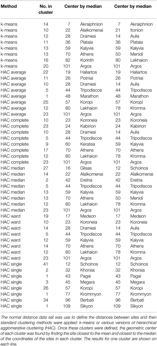
Table A2. Results of partitioning the data into eight clusters and then finding the geometric center.

FIGURE A1

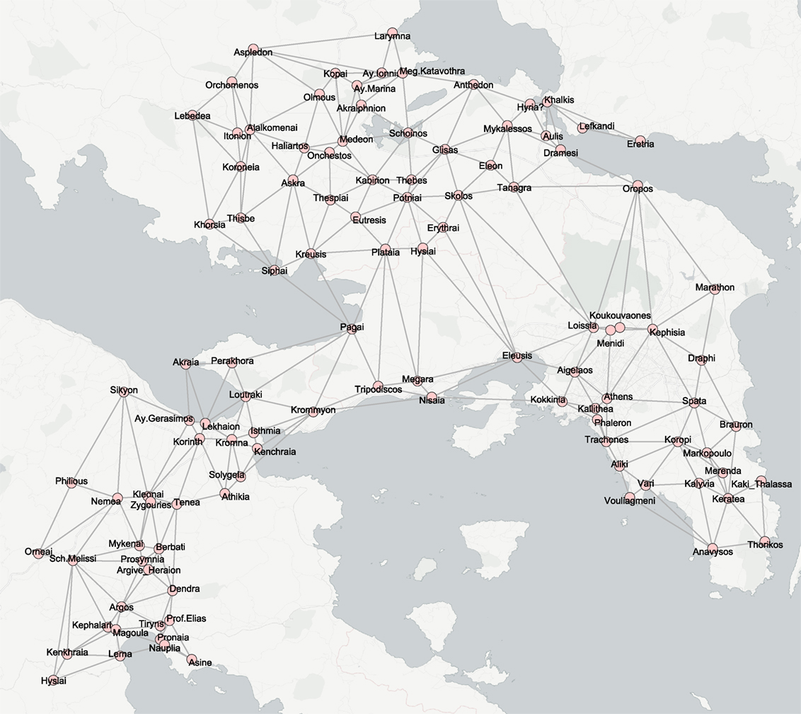
Figure A1. The approximate locations of the 109 sites used as the starting point for this study, derived from Figure 1 of Rihll and Wilson (1987). The index of site numbers is given in Table A1 in Appendix. Note that site 64, Vouliagmeni, was not labeled in the original figure, see Evans (2016a) for more details. The edges are those used to derive the second set of distances (denoted DTMedit) and are a subset of the edges of a Delaunay Triangulation.

FIGURE A2

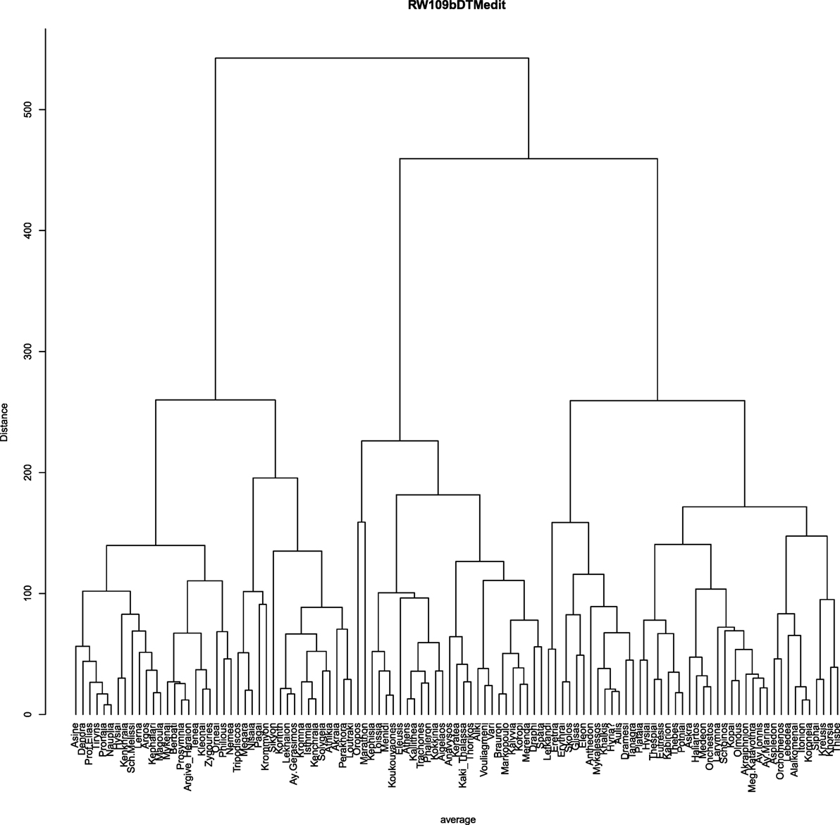
Figure A2. Hierarchical agglomerative clustering for distances based on the edited Delaunay Triangulation network (DTMedit) using average criterion for agglomeration.