Estimating Spring Terminus Submarine Melt Rates at a Greenlandic Tidewater Glacier Using Satellite Imagery

Introduction

Acceleration of marine-terminating glaciers in Greenland in recent decades has significantly increased the contribution of the ice sheet to sea level (Enderlin et al., 2014). Many of these glaciers are in contact with relatively warm ocean water (Holland et al., 2008; Straneo et al., 2012; Carr et al., 2013; Motyka et al., 2013), and submarine melting at the ice-ocean interface has been proposed as a potential trigger of glacier calving, retreat and acceleration (Nick et al., 2009; O'Leary and Christoffersen, 2013; Luckman et al., 2015). The spatial distribution of submarine melting along an ice front can impact grounding line stability and influence ice front shape by undercutting, overcutting, and creating embayments (Straneo et al., 2012; Carroll et al., 2015; Fried et al., 2015). These changes in ice front shape likely affect calving processes and can create locations along the ice front where calving preferentially occurs (Chauché et al., 2014; Luckman et al., 2015). The dynamic coupling between glacier margins and upstream ice enables oceanic forcing of tidewater glaciers to promote widespread thinning, increased glacier retreat, calving and velocity, and consequent mass loss (e.g., Joughin et al., 2004; van den Broeke et al., 2009; Vieli and Nick, 2011; Carr et al., 2013; Goelzer et al., 2013; Sundal et al., 2013; Straneo and Cenedese, 2015).

Despite their potential importance for ice dynamics, submarine melt rates (SMRs) are poorly constrained, because collecting in situ measurements near actively-calving glacier termini is both difficult and dangerous (e.g., Mortensen et al., 2011, 2013; Lea et al., 2014). Numerous studies have instead used hydrographic profiles from glacial fjords to estimate the net heat flux available for melting ice, resulting in SMRs up to 16.8 ± 1.3 m d⁻¹ in Alaska (Motyka et al., 2003, 2013) and ranging from 0.7 ± 0.2 to 10.1 m d⁻¹ in Greenland (Rignot et al., 2010; Sutherland and Straneo, 2012; Inall et al., 2014). Other studies have used general circulation models or plume theory to estimate SMR (e.g., Jenkins, 2011; Christoffersen et al., 2012; Sciascia et al., 2013; Xu et al., 2013; Slater et al., 2015), resulting in melt rates ranging from 0.12 to 3.6 m d⁻¹ in Greenland. However, most measurements used to estimate SMR from heat flux methods or to constrain model parameters are taken far from the grounding line (15–80 km away) (e.g., Johnson et al., 2011; Christoffersen et al., 2012; Sutherland and Straneo, 2012; Inall et al., 2014), and are therefore integrating all the processes that will affect the heat flux between the measurement site and the terminus, including heat lost to the melting of icebergs, sea ice, and mélange at considerable distances from the grounding line. SMRs estimated from fjord heat flux are also uncertain due to the temporal variability in fjord circulation, so that it is not clear how representative an estimate is of the longer term mean (Jackson and Straneo, 2016).

Alternative approaches to estimating glacier submarine melt rate utilize remotely sensed observations. Several studies have quantified SMR by accounting for ice flux divergence and surface mass balance of floating ice shelves and tongues (e.g., Rignot and Jacobs, 2002; Depoorter et al., 2013; Enderlin and Howat, 2013; Rignot et al., 2013; Gourmelen et al., 2017). This approach has generated SMRs up to 0.11 m d⁻¹ beneath ice shelves in Antarctica (Rignot and Jacobs, 2002) and ranging from 0.03 ± 0.02 to 2.9 ± 0.65 m d⁻¹ beneath floating glacier tongues in Greenland (Enderlin and Howat, 2013). Enderlin and Hamilton (2014) also used remotely sensed observations to estimate submarine melt, using changes in iceberg freeboard derived from high-resolution digital elevation models (DEMs) to estimate iceberg volume loss, which was then used to estimate area-averaged iceberg SMRs. During the summers of 2011 and 2013, estimated iceberg SMR was 0.39 ± 0.17 m d⁻¹ in Sermilik Fjord, east Greenland. Here we also employ a remote sensing approach, using satellite radar data to estimate near-terminus SMR from spatial and temporal changes in seasonal ice tongue freeboard adjacent to a large tidewater glacier in southwest Greenland.

Study Area

Located at the head of Kangersuneq Fjord (KF), Kangiata Nunaata Sermia (KNS), the largest tidewater glacier in southwest Greenland, drains ~2% of the ice sheet (Sole et al., 2011; Figure 1). The ice front is ~4.5 km wide with a maximum grounding line depth of ~250 m below sea level (Mortensen et al., 2013). KNS has retreated at least 22 km from its Little Ice Age maximum extent, following increased air and sea surface temperatures (Lea et al., 2014). For the past 15 years, with the exception of 2011 and 2015, a thick seasonal ice tongue contiguous with the glacier forms by mid-winter and advances down-fjord prior to rapid break-up in late-spring (Motyka et al., 2017; Figure 2). The floating ice tongue flows directly across the glacier grounding line (e.g., with no gap or calving processes occurring between the grounded and floating ice) with near spatially consistent velocity (see Supplementary Figures 1, 2). On average, the ice tongue has a length between 2 and 3 km, and decreases in freeboard with distance from the grounding line (Figure 2). The fjord waters adjacent to the front of the ice tongue are typically packed with dense ice mélange (i.e., mixture of sea ice, bergy bits, and icebergs) during the winter and spring months before breaking up in late spring.

FIGURE 1

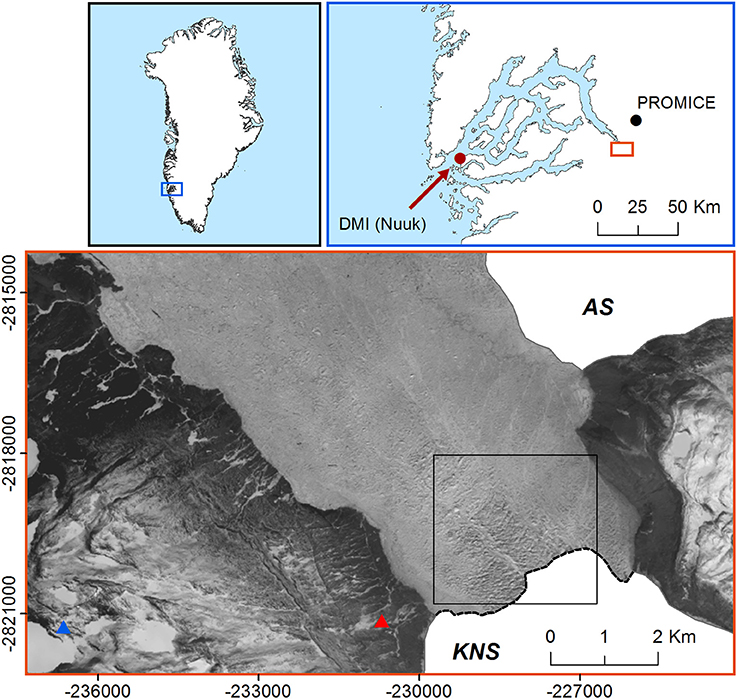
Figure 1. Map of study area, including Kangiata Nunaata Sermia (KNS) and Akullersuup Sermia (AS) glaciers and ice tongue and mélange, from Landsat 8 satellite image acquired for May 1, 2013 (bottom panel).The red and blue triangles indicate the locations of the University of Alaska Fairbanks (2013) and our (2009) time lapse cameras, respectively, and the black box indicates the extent of Figures 4A,B. The red and black dots in the fjord scale locator map (top right panel) indicate the locations of the Danish Meteorological Institute (DMI) and GEUS PROMICE weather stations, respectively.

FIGURE 2

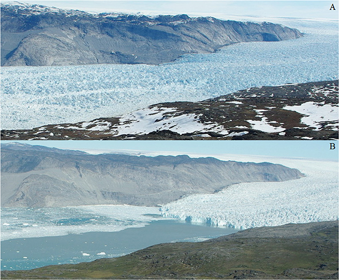
Figure 2. Example photographs from our 2009 time lapse camera (see Figure 1 for location) demonstrating (A) the intact ice tongue on 25 May 2009 and (B) the glacier terminus on 19 July 2009, post-ice tongue disintegration.

Mortensen et al. (2011, 2013) performed detailed analyses on the characteristics of the waters and heat sources entering KF and reaching to within ~4 km of the KNS terminus. Classical two-layered buoyancy-driven circulation operates in the fjord primarily during the spring and summer, where circulation is driven by subglacial meltwater plumes (Figure 3). Subglacial discharge exits the glacier at the grounding line, rises buoyantly along the ice front due to its lower density relative to the ambient fjord water, and flows down-fjord once neutral buoyancy is reached (Motyka et al., 2003; Jenkins, 2011; Cowton et al., 2015). In fjords with shallow glacier grounding line depths (<500 m) like KNS, summer discharge meltwater plumes often reach neutral buoyancy and horizontally enter the fjord within the upper 100 m of the water column (Carroll et al., 2016). The outflow forced by the subglacial discharge establishes an estuarine circulation cell, drawing in coastal waters from the shelf, which flow in a layer beneath the fresher outflow (Motyka et al., 2003; Mortensen et al., 2011). This warm coastal water is then entrained into the subglacial discharge plume, and melts the ice front and underside of the ice tongue as it rises.

FIGURE 3

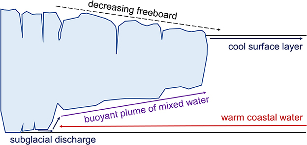
Figure 3. Schematic of intact ice tongue showing buoyancy-driven circulation in the fjord, as well as the characteristic decrease in ice tongue freeboard (and thus thickness) away from the ice front.

Data and Methodology

DEM and Ice Velocity Data Generation

We used TanDEM-X and TerraSAR-X imagery from 2013 to estimate ice tongue freeboard and velocity, respectively. TerraSAR-X has a repeat period of 11 days and both satellites have spatial resolution on the order of a meter (Krieger et al., 2007; Eineder et al., 2011), thereby providing excellent temporal and spatial resolution for observing changes in ice tongue velocity and freeboard. The radar platforms enabled us to use imagery acquired in non-daylight hours and cloudy conditions, in contrast to optical platforms. Time lapse camera imagery near the terminus of KNS (Figure 1) every 4 h from January to June 2013 (courtesy of M. Truffer and M. Fahnestock, University of Alaska Fairbanks) was used to visually confirm the formation, presence, and break-up of the ice tongue.

We derived two 2.5 m resolution DEMs dated 17 March and 27 May 2013 from conventional SAR interferometric processing of bi-static TanDEM-X imagery (Dehecq et al., 2016). GIMPDEM (Howat et al., 2014) was used as a reference during the unwrapping stage to minimize unwrapping errors. The DEMs produced must be correctly aligned, both horizontally and vertically, using known stable areas (e.g., bedrock outcrops) that are not covered by ice or snow. To perform this calibration, we used ICESat elevation data over non-ice terrain as defined by the GIMP land classification mask (Howat et al., 2014). A horizontal shift (3.9 and 3.3 m in the x and y directions, respectively) between the TanDEM-X derived DEMs and ICESat over non-ice covered terrain was calculated by fitting a sinusoidal relationship between elevation differences and terrain aspect (Nuth and Kääb, 2011). A vertical shift with a linear dependence on location (tilt) was estimated for each DEM using a least-squares regression:

$\begin{array}{ll}dh(X,Y)=a_0+a_{1}X+a_{2}Y& (1)\end{array}$

where dh are elevation differences in stable areas, X and Y the easting and northing and a_i the parameters to be estimated. This shift was then subtracted at each pixel. For this step, which is more sensitive to outliers, all points with a slope higher than 40° were excluded. The DEMs were then converted from ellipsoid to elevation above the EIGEN-EC4 geoid.

Due to the limited coverage of the ICESat lines over non-ice terrain (see Supplementary Figure 3), an additional tilt in the DEMs was identified and subsequently corrected for using Operation IceBridge (OIB) Airborne Topographic Mapper (ATM) L1B Elevation and Return Strength data (Krabill, 2016). OIB ATM elevation points were acquired for three springs when the seasonal ice tongue was present in the fjord (08 April 2011, 25 April 2012, and 15 April 2014). TanDEM-X elevations from 17 March 2013 were extracted for spatially corresponding 2011 OIB ATM points and the difference taken over open water where the OIB data had a slope of near-zero (20 to 25 km from the ice front). The slope of the difference was taken as the trend (or tilt; ~0.45 m height per km distance along-fjord) in the TanDEM-X elevations and was removed, effectively de-trending the dataset (see Supplemental Figure 4). The same correction was applied to elevations from the 27 March 2013 DEM, as the tilt was the same as that for the 17 March.

Three 20 m resolution ice tongue velocity maps were created based on conventional feature tracking applied to TerraSAR-X imagery (Tedstone et al., 2014) for the following 2013 image pairs: 12–23 February, 8–19 April, and 30 April to 11 May. Ice velocity on 17 March (Supplemental Figure 1A), the date of our first DEM, was estimated assuming a linear trend in velocity between the velocity maps from 12–23 February to 8–19 April, and ranges from 28.5 to 30.5 m d⁻¹ over the ice tongue. The last available velocity map was from 30 April to 11 May (Supplemental Figure 1B), and throughout the paper, we use this velocity epoch to correspond with our second DEM, acquired on 27 May. Ice tongue velocities in May range from 20.5 to 23.5 m d⁻¹.

Ice Flowline Construction

We constructed flowlines along the ice tongue using our ice velocity results to track flow direction. Ten points near the glacier grounding line were chosen from both the eastern and western side of the ice tongue, with ~25 m between points in the across-flow direction (Figure 4). To accommodate temporal changes in ice velocity, two separate sets of flowlines were created, one for March and one for May, using our velocity maps from 17 March and 30 April to 11 May, respectively. Velocity vectors were extracted for each initial point, enabling the extraction of flow direction, which was then taken at points every 50 m moving down-fjord until the end of the ice tongue. The points were then connected, creating flowlines of ice moving down-fjord away from the grounding line (Figure 4). Distance from the grounding line was averaged for each set of flowlines (i.e., eastern and western), using the end of spring terminus position (Figure 1) digitized from a Landsat 8 image from 10 June 2013.

FIGURE 4

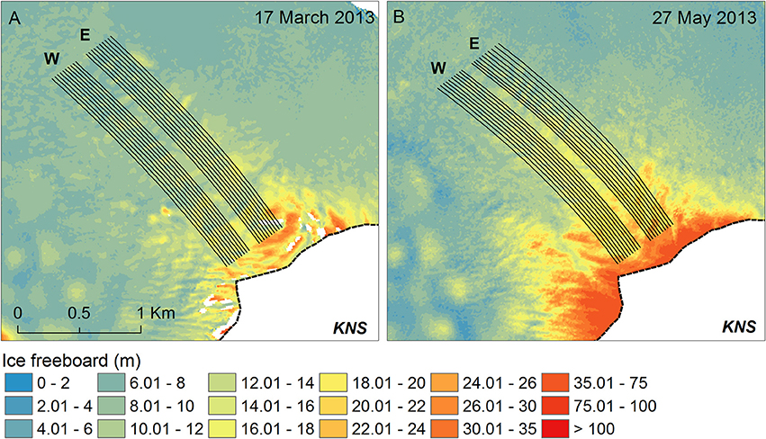
Figure 4. Eastern (E) and western (W) ice flowlines, overlain on TanDEM-X ice tongue freeboard from (A) 17 March 2013 and (B) 27 May 2013. Refer to Figure 1 for location.

Estimating Ice Tongue Surface Melt Rates

Observed reduction in ice tongue freeboard as it is advected into the fjord can be attributed to changes in surface mass balance, longitudinal and lateral spreading, and submarine melting. To assess the potential contribution from surface mass balance, surface melt was estimated using a simple positive degree day (PDD) model (Hock, 2003) with a degree day factor for snow (ddfs) of 4.5 mm d⁻¹ °C⁻¹, as used by Slater et al. (2017) for KNS. Air temperature (°C) data were acquired from the nearby Geological Survey of Denmark and Greenland (GEUS) PROMICE weather station (NUK_L, 550 m a.s.l., 64°28′55.2″ N, 49°31′50.88″ W, ~21 km from KNS) (Ahlstrom et al., 2008; Figure 1), using a lapse rate of 0.5°C per 100 m to adjust the temperatures to sea level (Slater et al., 2017). Precipitation data were acquired from the Danish Meteorological Institute (DMI) weather station in Nuuk (NUUK 4250, 80 m a.s.l., 64°10′0.12″ N, 51°45′0″ W, ~105 km from KNS) (Cappelen, 2016; Figure 1).

Estimating Submarine Melt Rate (SMR)

SMR for all ice flowlines were estimated for both steady and non-steady state scenarios. A steady state scenario assumes ice thickness at a fixed location does not change in time, whereas a non-steady state scenario allows for changes in ice thickness at a fixed location (e.g., thinning due to high submarine melting exceeding the delivery of ice across the grounding line or changes in the thickness of ice being advected across the grounding line). As estimating a non-steady state scenario requires at least two elevation estimates, a steady state (i.e., ∂H/∂t = 0) is often assumed due to lack of data (e.g., Jenkins and Doake, 1991; Smith, 1996; Johnson et al., 2011). The two scenarios are presented here for comparison purposes, in part to test the validity of our method for years with only one DEM, when determining SMR by assuming a steady state scenario would be the only option. For a steady state scenario (SS), elevation values along each ice flowline were extracted from both the 17 March and 27 May 2013 DEMs. To reduce the impact of short-length scale elevation changes, including crevasses, in the fractured tongue (see Figure 2) on our melt rate estimates, flowline elevations were smoothed using a two-sided moving average with a 625 m window (see Figures 5A, 6A). Elevation data were then converted to ice thickness using ocean water (1,027 kg m⁻³; Ribergaard, 2013) and ice (900 kg m⁻³ following Enderlin and Hamilton, 2014) densities, assuming the ice is floating in hydrostatic equilibrium; an assumption supported by both the best available bathymetry (Mortensen et al., 2013; Motyka et al., 2017) and the observation of the rapid and total disintegration of the ice tongue within just a 4-h time window on 15 June 2013.

FIGURE 5

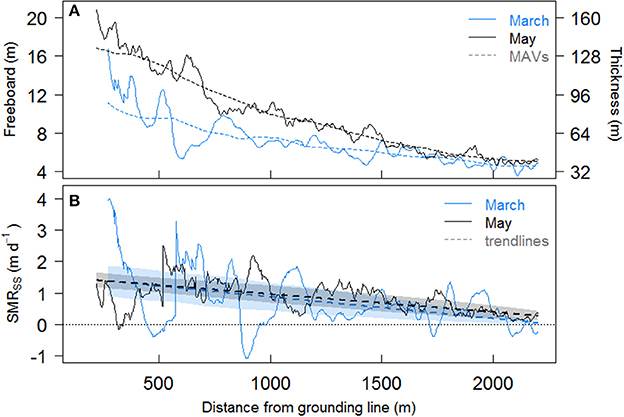
Figure 5. (A) Ice freeboard and thickness (m) on 17 March and 27 May 2013 with distance from KNS terminus for the eastern flowlines, where solid lines are means from 10 flowlines (Figure 4) and dashed lines are moving averages (MAVs) of the mean; (B) Steady state estimated submarine melt rate (SMR_SS) for eastern flowlines, with dashed trendlines and shaded error ranges.

FIGURE 6

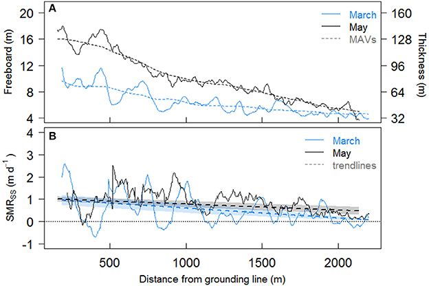
Figure 6. (A) Ice freeboard and thickness (m) on 17 March and 27 May 2013 with distance from KNS terminus for the western flowlines, where solid lines are means from 10 flowlines (Figure 4) and dashed lines are moving averages (MAVs) of the mean; (B) Steady state estimated submarine melt rate (SMR_SS) for western flowlines, with dashed trendlines and shaded error ranges.

SMR_SS were calculated for both March and May, accounting for thinning due to stretching in both the flow direction (second term on right-hand side of Equation 2) and perpendicular to flow (third term on right-hand side of Equation 2):

$\begin{array}{ll}SM{R}_{SS}=-v_x\frac{\partial H}{\partial x}-H\frac{\partial v_x}{\partial x}-H\frac{\partial v_y}{\partial y}& (2)\end{array}$

where H is the ice thickness (m), v_x and v_y are the ice velocity (m d⁻¹) in the along- and across-flowline direction, and x and y represent distance in the along- and across-flowline direction.

Note that a term representing across-flow thinning, ${-v}_y\frac{\partial H}{\partial y}$, does not contribute because, by definition of a flowline, v_y = 0 on the flowline. The final term in Equation (2) does however make a small contribution due to the convergence or divergence of different flowlines. Derivatives in Equation (2) are evaluated using conventional finite differences with a spacing Δx = 50 m and Δy = 25 m.

For a non-steady state scenario (NSS), a linear trend of thickness change between 17 March and 27 May 2013 was assumed at each point on the flowlines and accounted for by subtracting a daily rate of change (m d⁻¹) from the estimated SMR_SS (Rignot et al., 2013):

$\begin{array}{ll}SM{R}_{NSS}=SM{R}_{SS}-\frac{\Delta H_{NSS}}{\Delta t}& (3)\end{array}$

where ΔH_NSS (m) is the difference in ice thickness between the two dates and Δt (d) is the time between the two dates.

Melt rates were then averaged to produce a mean SMR_SS and SMR_NSS for the western and eastern flowlines. To capture the general trend in melt rates, lines of best fit were applied to both steady and non-steady state estimates.

Error Analysis

Potential errors were traced throughout the analysis and standard error propagation methods were used to calculate the effect of errors in both elevation and ice velocity on estimated SMR. Errors in elevation values are from three primary sources: (1) DEM construction (including correction using ICESat), (2) correcting TanDEM-X elevations using OIB ATM data, and (3) smoothing the elevations for melt rate calculations. Error resulting from DEM construction is ±2 m, a general error for the TanDEM-X derived DEMs over areas with a slope <12° (Rizzoli et al., 2012), which is likely an overestimate over the relatively low-sloped ice tongue (<0.15°). As our calculations utilize the elevation gradient and not the absolute elevation, we instead account for a gradient error of ±0.35 m over the nearly 2 km ice tongue. This gradient error was estimated over 2 km segments (the same length over which SMRs were estimated) of a section of very thin ice mélange where successive OIB ATM flights show near-constant slope. The gradient error was estimated as the largest difference in slope between the corrected TanDEM-X elevation flowlines and the OIB ATM lines. Fitting the TanDEM-X elevations to the OIB ATM elevations results in a root mean square error of ±0.38 m, and smoothing the flowlines results in maximum mean squared errors of ±0.86 and ±0.47 m for the eastern and western flowlines, respectively. The maximum total error for any one point in elevation along the eastern and western flowlines is ±1.4 and ±0.64 m, respectively.

Following Paul et al. (2015), error in ice velocity was estimated as ±0.09 m d⁻¹, resulting from the feature tracking process applied to stable areas of the ice tongue, where crevassing is easily trackable and ice deformation is low. Errors in velocity at locations within 150 m of the original position of the previous end of summer vertical ice-front (which likely corresponds to the grounding line) and at the edge of the ice tongue are not considered, as we did not use any velocities from these regions in our SMR estimations.

While the error estimates cited alongside our SMRs account for errors in the DEMs and ice velocity maps, there are several additional sources of error that, although difficult to quantify, must be considered. The assumption of both steady and non-state state scenarios for ice tongue thickness likely introduces error in our SMR estimates. We know the ice tongue is not in steady state between March and May 2013, as the glacier is slower and the ice is thicker in May than in March for any given point. Since we have only two DEMs, we can only assume a linear thickening trend over the time period (see Equation 3). Any deviation from this trend would affect our melt rate estimates. For example, if the ice tongue was thickest in April, this would imply the ice tongue was thinning between April and May, increasing NSS melt rates estimated using Equation 3. Thus, if the tongue was thickest in April, our May melt rate estimates would be an underestimate; however without additional DEMs we cannot address this possibility.

Another potential source of error derives from smoothing the ice freeboard near the glacier grounding line, where pre-smoothed freeboard values decrease sharply, as compared with smoothed values (see Figures 5A, 6A). While smoothing out fracturing associated with large crevasses on the ice tongue helps to reduce noise in the SMR estimates, the resultant reduction in freeboard gradient significantly lowers our SMRs near the grounding line, which should therefore be considered minimum estimates of melt rate in this location.

Results

SMR Estimates in Kangersuneq Fjord

The reduction in smoothed ice freeboard (and thus thickness) with distance down-fjord from the grounded KNS terminus in the March DEM (Figures 5A, 6A for eastern and western flowlines, respectively), combined with the interpolated ice velocities, results in SMR_SS for the eastern and western flowline sets of up to 1.4 ± 0.5 m d⁻¹ (mean = 0.7 ± 0.4 m d⁻¹) and 1.0 ± 0.2 m d⁻¹ (mean = 0.5 ± 0.2 m d⁻¹), respectively (see lines of fit in Figures 5B, 6B). Due to thickening of the ice via advection, estimated SMR_NSS for each set of flowlines (not shown) are less than those estimated for the steady state scenario, with mean decreases in melt rate of 15 and 28% for the eastern and western flowlines, respectively. For all flowlines, melt rates broadly decrease with distance from the KNS grounding line and moving from east to west across the ice tongue.

SMR_SS estimated in May are similar to those in March, with eastern and western flowline SMRs of up to 1.4 ± 0.2 m d⁻¹ (mean = 0.8 ± 0.3 m d⁻¹) and 1.0 ± 0.1 m d⁻¹ (mean = 0.7 ± 0.3 m d⁻¹), respectively (see lines of fit in Figures 5B, 6B). Estimated SMR_NSS for each set of flowlines are again less than those estimated for the steady state scenario, decreasing by 3 and 10% for eastern and western flowlines, respectively. SMRs in May show the same spatial variability as seen in March.

While the heavily crevassed nature of the ice tongue itself is not unphysical, it leads to unphysical noise in our melt rate estimates. For example, the rapid decrease in thickness between two adjacent points over a crevasse (one on the ice tongue surface and one at the bottom of the crevasse) is interpreted as thinning using our method, and thus the estimated SMR would be erroneously high (e.g., the peak in March SMR ~570 m from the grounding line, Figure 5B). In contrast, the rapid increase in thickness between a point at the bottom of the same crevasse and ice tongue surface on the other side is interpreted as thickening of the ice, resulting in a negative melt rate (e.g., negative March SMRs, Figure 5B). To exclude these anomalous melt rates, we use the lines of best fit as seen in Figures 5B, 6B to interpret the broader trends in estimated SMR. As they are the same order of magnitude as the non-steady state scenario, we use our steady state scenario melt rates in our subsequent analyses, which allows for comparison to melt rates estimated in years when only one DEM is available (i.e., assumed steady state). In addition, we note again that our melt rates near the grounding line should be considered minimum estimates, as the smoothing of crevasses greatly reduces freeboard gradient here.

Surface Melt Estimates over the Ice Tongue

For the study period, between 17 March and 27 May 2013, total surface snow melt over the ice tongue was 0.48 m water equivalent and total precipitation as snow was 0.23 m. We expect precipitation to be less over the ice tongue than that recorded in Nuuk, given the low elevation of the ice tongue and the rain shadow effect of the coastal mountains. A previous study estimated spring average precipitation decreases between coastal and inland weather stations in western Greenland between ~0.5 and 0.8 mm per km inland (Abermann et al., 2017). Therefore, if anything, by using the estimates of precipitation from Nuuk we overestimate spring snowfall. Regardless, the estimates of precipitation are still orders of magnitude lower (in terms of water equivalent and impact therefore on freeboard) than our estimated SMRs. The resultant mean surface melt rate, 0.004 m d⁻¹, taken over the 71 days of the study period, is approximately two orders of magnitude less than the rate of change in ice thickness over the same time period, and thus considered negligible. As the PDD sum for 2013 during our study period (16.3°C day) is ~75% lower than the mean for the last decade (mean from 17 March to 27 May for 2008 to 2016 of 69.4°C day), 2013 should be considered a low spring surface melt and runoff year.

Discussion

Spatial Variability in SMR

Submarine melt rates show along-fjord variability, generally decreasing with distance down-fjord from the KNS grounding line. This variability is likely driven by both the velocity and temperature of subglacial meltwater plumes, with SMR scaling with velocity and ambient fjord temperature (e.g., Holland and Jenkins, 1999; Jenkins, 2011). Mortensen et al. (2013) investigated winter circulation and water properties in 2009 in KF, finding a cool surface layer (ranging from −1.4 to 1.0°C at 0 and 40 m depth, respectively) overlaying a warmer intermediate-depth layer (increasing from 1.3 to 1.8°C at 50 to 90 m depth), below which temperature was relatively constant (1.8°C) with depth. Motyka et al. (2017) investigated summer fjord water properties in 2011, ~22 km from the KNS ice front, again finding a cool surface layer (ranging from 0 to 1.0°C at 0 and 40 m depth, respectively) overlaying an even warmer intermediate layer (increasing from 2.0 to 2.5°C at 50 to 150 m depth). Therefore, the ambient fjord water entrained by any subglacial plumes will be cooler with increasing distance from the grounding line, as the thinning ice tongue, and shallower draft, will be submerged in shallower, colder surface water. Plume velocity also decreases with distance from the ice front as the plume loses buoyancy (Jenkins, 2011). For these reasons, and as expected, our estimated SMRs approach 0 m d⁻¹ down-fjord of the grounding line. The presence of thick sea ice down-fjord of the end of the ice tongue supports this expectation, suggesting the surface waters are very cold, resulting in little or no submarine melting (or else there would be no sea ice). This result is dissimilar to summer melt rates derived from icebergs found tens of kilometers from glacier grounding lines in other Greenlandic fjords (Enderlin and Hamilton, 2014), which we would expect to be higher, due to deeper iceberg keel depths (as compared to the shallow ice tongue depth) and stronger buoyancy-driven circulation from higher subglacial discharge in the summer (Sciascia et al., 2013).

SMRs also show across-fjord variability, with higher melt rates in the eastern section of the main ice tongue, compared to the western part. Across-fjord variability may be driven by water temperature, both in the ambient water column and thus the plume, and by the strength (i.e., velocity) of any buoyant runoff plume present. The eastern part of the ice tongue had the highest March surface elevation, and thus the greatest thickness and deepest keel depth (Figure 5A). Reaching over 80 m beneath the fjord surface near the grounding line, ice along the eastern flowlines is exposed to relatively warm, intermediate-depth waters, which promote more rapid submarine melting (Enderlin and Hamilton, 2014; Enderlin et al., 2016). In comparison, ice in the western part of the tongue has a keel depth near the ice front of <70 m, which could explain, in part, the lower SMR in this area of the fjord, as the shallower ice keel is exposed to slightly cooler waters than the eastern part of the tongue.

Across-fjord variability in SMR may also reflect the strength and location of any subglacial meltwater plumes emerging at the glacier grounding line. Uniform across-fjord ice tongue SMR would be expected, if keel depths are constant, where spatially well-distributed meltwaters emerge at the grounding line (Slater et al., 2015). Conversely, spatially-focused, high SMRs near the ice front may indicate a locally dominant subglacial meltwater channel, which in this case could be emerging preferentially under the eastern part of the ice tongue. Slater et al. (2017) inferred KNS subglacial runoff distribution using plume observations from summer 2009 time lapse imagery, suggesting that runoff likely exits under the grounding line via spatially distributed channels, with sporadic focusing resulting in visible surface plumes. During the mid- to late melt season, plumes typically reach the surface to the west of the grounding line center, with infrequently visible plumes emerging on the eastern side of fjord (Slater et al., 2017). However, as the presence of the ice tongue and surrounding thick ice mélange prevents the expression of plumes on the surface, it is difficult to interpret subglacial meltwater distribution during the winter and spring months.

In addition, rotational circulation in the fjord should be considered, which could impact the across-fjord distribution of surface meltwater and water entering the fjord at depth (Cottier et al., 2010; Straneo and Cenedese, 2015), and thus the heat available for melting ice. Using data from Mortensen et al. (2013), we assume a 30 m thick fresh surface layer of sea ice/ice tongue/glacier meltwater overlaying transitional layers of ice melt and fjord source water, which gives an internal Rossby radius of ~6 km. As the fjord width varies between 4 and 6 km, rotational effects are unlikely to have a primary role in controlling fjord circulation. However, they may have a secondary effect, focusing the flow of water toward and away from the glacier terminus to the right hand side in the direction of flow (e.g., Cottier et al., 2010; Sutherland et al., 2014).

Temporal Variability in SMR

Estimated mean SMRs do not show significant temporal variability, potentially due to the fact that all melt rates are estimated in the spring, prior to the on-set of substantial surface melt. While estimated monthly total surface snow melt from degree day modeling was higher in May (0.26 m) than in March (0.11 m), we do not expect or see significant differences in SMRs given how small these early spring surface melt rates are. However, increased surface melt later in the melt season and the associated enhanced subglacial meltwater plumes, combined with increased intermediate depth water temperatures (Mortensen et al., 2013; Motyka et al., 2017) would be expected to amplify local SMR considerably compared to winter melting (Jackson and Straneo, 2016). Such estimates would however not be possible using our method as the ice tongue breaks up in early June each year, and is thus absent during the summer and autumn months.

Seasonal stratification and water temperature at depth are highly dependent on the mode of circulation in KF (Mortensen et al., 2011). In the spring, when we estimate SMR, circulation is mainly driven by dense coastal inflows and tidal mixing, which act to cool and slightly freshen waters at intermediate depths. The presence of subglacial meltwater plumes sourced from frictional basal meltwater emerging at the glacier grounding line (Christoffersen et al., 2012) likely also play a role in controlling fjord circulation and submarine melting in the winter and early spring. In the summer, however, tidal mixing and subglacially-driven circulation, via surface-derived meltwater plumes, are dominant and act to freshen and significantly warm the upper intermediate water layer (Mortensen et al., 2013). Temperature differences of nearly 2°C were seen at intermediate depths (between 120 and 150 m) between April and September 2010 (Motyka et al., 2017), an increase which would have a significant impact on the melting of submerged ice.

In order to investigate the potential role that basal frictional meltwater could play in driving plumes in winter, we estimate basal meltwater flux for the area of KNS between the grounding line and ~11 km up-ice from the grounding line. As basal drag is unknown for KNS, we assume drag is of a similar magnitude to that estimated for Jakobshavn Isbræ, ~200 kPa (Iken et al., 1993; Funk et al., 1994), as used for Kangerdlugssuaq Glacier by Christoffersen et al. (2012). Using our TerraSAR-X derived velocities for March and May for the lower 11 km of the glacier, an ice density of 900 kg m⁻³, and a latent heat of fusion of 334 kJ kg⁻¹, basal meltwater flux was estimated as 3.2 m³ s⁻¹, for both March and May. Although producing weak plumes, subglacial discharge of this magnitude can generate point source SMRs of between 2 and 4 m d⁻¹ (Slater et al., 2015). Due to their lower velocity, weak plumes, such as those expected via basal frictional melting, reach neutral buoyancy before reaching the fjord surface (Christoffersen et al., 2012; Slater et al., 2015; Carroll et al., 2016). However, close to the glacier grounding line, where ice tongue keel depth is greatest, weaker plumes will likely still reach and melt the base of the ice tongue. In comparison, higher subglacial discharge (between 50 and 100 m³ s⁻¹), as might be expected later in the melt season, can result in point source SMRs up to 7 m d⁻¹ (Slater et al., 2015). These stronger plumes may reach the fjord surface before reaching neutral buoyancy, thus allowing for melting of the full ice front depth (Slater et al., 2015).

Comparison with Previous SMR Estimates from Greenland

Submarine melt rates estimated in this study are greater than, but of the same order of magnitude, as those estimated for icebergs during summer in Sermilik Fjord, southeast Greenland. Using repeat high-resolution satellite imagery, Enderlin and Hamilton (2014) estimated SMRs of 0.39 ± 0.17 m d⁻¹ for icebergs located up to 60 km from the terminus of Helheim Glacier between August 2011 and July 2013. Using our lines of best fit, our estimated SMRs (up to 1.4 m d⁻¹) are more than double those of Enderlin and Hamilton (2014). Given the close proximity to the grounding line, our estimated SMRs may reflect the influence of melting by plumes enhanced by emerging subglacial meltwater sourced from frictional basal melt (e.g., Christoffersen et al., 2012); such plumes will clearly have a diminished influence 60 km from the ice front, where plume velocity has decreased. Estimated SMRs for icebergs stuck in ice mélange in Sermilik and Ilulissat fjords range from 0.1 to 0.8 m d⁻¹, and increase with iceberg draft and submerged ice area (Enderlin et al., 2016). These melt rates are more similar to ours near KNS, due both to the relatively similar distance from the grounding line to the icebergs (from 0 to 20 km away) and our estimates (150 to 2,400 m away), as well as the comparable summer intermediate ambient water temperatures in Ilulissat (up to 2.2°C) (Mernild et al., 2015), Sermilik (up to 2°C) (Straneo et al., 2010, 2011), and Kangersuneq (up to 2.5°C) fjords.

Estimated SMRs for the KNS ice tongue in spring 2013 are one to two orders of magnitude larger than SMRs estimated between 2000 and 2010 for the floating tongue at Petermann Glacier (0.07 ± 0.035 m d⁻¹) (Johnson et al., 2011; Enderlin and Howat, 2013). The difference in melt rate magnitude in this case is likely due to both the difference in ambient ocean temperatures at ice keel depth between the two fjords as well as meltwater plume dynamics. The ambient water temperatures in northwest Greenland are much lower at keel depth than those in southwest Greenland, peaking at 0.2°C at nearly 500 m depth in Peterman Fjord (Johnson et al., 2011), where keel depths in the first few km of the fjord reach ~480 m (Wilson et al., 2017). In contrast, ambient water temperatures at keel depth for KNS (~80 m near the grounding line) fall between 1.3 and 2.0°C, depending on the season (Mortensen et al., 2013; Motyka et al., 2017). Plume dynamics may also fundamentally differ, with the weak melt-driven convective plumes beneath Petermann (which has a ~70 km long permanent ice tongue) more akin to those at large Antarctic ice shelves, and strong subglacial discharge-driven plumes beneath the short ice tongue at KNS giving rise to convection-driven melt as observed at tidewater glaciers in mid-summer (Jenkins, 2011). In addition, the difference in velocity between KNS and Petermann glaciers may play a secondary role in controlling estimated SMRs. The average winter velocity for KNS is ~8 km a⁻¹, eight times that of Petermann Glacier (Johnson et al., 2011). A faster-flowing, warm based glacier will create more basal friction and thus more basal melt (e.g., Holland et al., 2008; Christoffersen et al., 2012), producing more vigorous subglacial meltwater plumes and inducing higher SMRs even in winter (Carroll et al., 2015; Cowton et al., 2015; Slater et al., 2015).

Utilizing summer hydrographic observations between ~35 and 88 km from the Kangerdlugssuaq Glacier terminus, Inall et al. (2014) estimated heat delivery to the calving front equivalent to 10 m d⁻¹ of ice melt. Motyka et al. (2017) used parameters derived from models and hydrographic measurements 12 km from the KNS ice front to estimate a near-terminus late-summer SMR of ~3–7 m d⁻¹. Our empirically-derived SMRs are nearly an order of magnitude lower than those estimated by Inall et al. (2014) and the upper range estimates of Motyka et al. (2017), despite similar ambient fjord water temperatures (up to 2.25°C at depth for Kangerdlugssuaq Fjord; Inall et al., 2014). It is unlikely that hydrographic estimates taken more than 30 km from the terminus realistically represent the heat energy used for melting the ice front, as a large portion of this energy might be lost to melting of any ice mélange and icebergs in the fjord before reaching the glacier (Enderlin et al., 2016). In fjords like Helheim, where icebergs are large enough to cover the full fjord depth (Enderlin and Hamilton, 2014), deep water could also be cooled by the melting of icebergs at depth. Heat transport to the ice front can also be reduced through vertical mixing of the water column via wind-driven internal seiches (e.g., Arneborg and Liljebladh, 2001; Cottier et al., 2010) or by the convective overturning of water due to the release of brine from sea ice formation (Cottier et al., 2010). In addition, the presence of shallow sills in the fjord alter the fjord circulation and may prevent deeper, warm water from reaching the ice front (e.g., Mortensen et al., 2011, 2013). This suggests that terminus melt rates derived from distal along-fjord heat flux values may be too high unless the heat lost to mid-fjord melting, vertical mixing, and fjord bathymetry are considered.

Freshwater Flux from Submarine Melting of the Ice Tongue

Given the potential importance of meltwater generation to fjord water properties and nutrient productivity (Meire et al., 2017), we here estimate the spring freshwater flux from submarine melting of the ice tongue. Using grounded terminus width (~4,500 m), depth (~250 m), and average velocity from March to May 2013 (~6.9 km a⁻¹), spring ice flux across the KNS grounding line was estimated to be 246 m³ s⁻¹. Assuming a simplified rectangular submarine configuration of the ice tongue with a width of ~1,800 m and a length of ~2,500 m, total basal submerged area is ~4.5 km². Using spatially averaged SMR_SS from our western and eastern fjord flowlines, meltwater flux derived from the ice tongue ranges from 26 to 36 m³ s⁻¹ (11 to 15% of spring grounding line ice flux) in March, and from 36 to 42 m³ s⁻¹ in May (15 to 17% of spring grounding line ice flux). This partitioning of freshwater flux entering the fjord is comparable to that estimated by Xu et al. (2013) for Store Glacier in western Greenland, where submarine melting accounted for 20% of August 2010 glacier influx. In contrast, our flux partitioning is much lower than that estimated by Motyka et al. (2003, 2013) for LeConte Glacier in Alaska, where submarine melting accounts for 50–67% of summer frontal ablation. Differences in flux partitioning are likely due to seasonality and fjord temperatures, and to terminus geometry (Truffer and Motyka, 2016).

While ice tongue melt only accounts for ~11–17% of the overall spring grounding line flux, it provides a significant amount of freshwater to the fjord in spring months, when surface runoff is largely absent. As such, the associated inputs of freshwater into the fjord at different depths from submarine melting may have a major impact on fjord water stratification, circulation and associated productivity (e.g., Motyka et al., 2013; Sciascia et al., 2013; Sutherland et al., 2014; Meire et al., 2017).

Potential Applications

We have derived SMRs using changes in the freeboard of a seasonally floating ice tongue as it advances down-fjord during the spring, building upon earlier work using freeboard and ice flux divergence to estimate SMRs of floating ice tongues in Greenland (e.g., Motyka et al., 2011; Enderlin and Howat, 2013). This technique has considerable potential to further our understanding of ice-ocean interactions and submarine melting in glacial fjords. Using both satellite and time-lapse imagery, seasonal differences in SMR could be evaluated by estimating melting throughout the year, as long as an ice tongue is present in winter and spring, and icebergs are present in summer and autumn sufficiently close to the ice front (following methods of Enderlin and Hamilton, 2014). In addition, analysis of seasonally floating ice tongues presents the opportunity to derive SMR estimates much nearer to glacier calving fronts (when compared with estimates using hydrographic profiles), in the precise location where the key processes controlling calving dynamics and retreat are not well resolved. We anticipate that our estimates of SMR, and others derived using this methodology, will be used to tune fjord circulation and plume models, which in turn will soon be used to force ice sheet models predicting the future of the Greenland Ice Sheet and its contribution to sea level rise.

Our submarine melt rate estimates are derived from an ice tongue that is already floating, thus they do not affect the annual mass balance of the grounded portion of KNS. Nevertheless, the submarine melting of the ice tongue may affect its ability to buttress the winter ice flux and discharge across the grounding line (e.g., Motyka et al., 2011; Krug et al., 2015), with potential negative consequences for annual mass balance. If SMRs increase in the future as is expected under climate projections, the residence time of seasonal ice tongues like that at KNS will decrease, effectively extending the length of the calving season and allowing for greater mass loss from the grounded portion of the ice sheet. In addition, quantifying ice tongue melt rates can tell us a lot about calving front melt processes. For example, the spatial distribution of ice front SMRs (for which our ice tongue SMRs are a proxy) can influence the morphology of the calving front through spatially heterogeneous undercutting, with potential implications for calving frequency and style (Straneo et al., 2012; Chauché et al., 2014; Carroll et al., 2015; Slater et al., 2017), and ultimately glacier retreat, velocity and ice flux. A better understanding of spatial variations in submarine melting of the ice front may lead to the development of a relationship between melt distribution and calving, which is poorly understood but likely of critical importance for controlling tidewater glacier dynamics.

Conclusions

Improved estimates of SMR are essential to gain a better understanding of the processes controlling ice dynamics at tidewater glacier termini, and in particular, the potential relationship between submarine melt and tidewater glacier acceleration and retreat. Using high-resolution TerraSAR-X and TanDEM-X satellite imagery, we have estimated SMRs of a seasonal floating ice tongue adjacent to the grounding line of KNS. Changes in freeboard of the ice tongue, both with distance from the grounding line and across the fjord, have been used to estimate spatial variations in melt rate.

Our estimates of spring steady state SMR near the grounding line of KNS reach 1.4 ± 0.5 m d⁻¹, and decrease with distance down-fjord from the glacier grounding line, with mean rates up to 0.8 ± 0.3 and 0.7 ± 0.3 m d⁻¹ for the eastern and western parts of the ice tongue, respectively. There is also considerable across-fjord variability in SMR which may be driven by variation in the ice tongue draft and the temperature stratification in the fjord, but may also reflect the strength of any subglacial meltwater plumes present. The submarine meltwater flux derived from the ice tongue ranges from 26 to 42 m³ s⁻¹, which accounts for between 11 and 17% of the grounding line ice flux into the fjord in the spring months, prior to the onset of ice sheet surface melt. Our results demonstrate that using high resolution satellite imagery to analyze changes in freeboard at floating seasonal ice tongues has considerable potential to reveal in detail the temporal and spatial variations in SMR at tidewater glacier termini.

Author Contributions

AM performed all of the analysis and led the writing of the manuscript. NG produced the DEMs and ice velocities. All authors contributed ideas and methodological developments, and provided editorial input on the manuscript.

Funding

AM is supported by a Principal's Career Development PhD Scholarship from the University of Edinburgh. We acknowledge NERC grants NE/K015249/1 (to PN) and NE/K014609/1 (to AS), and a NERC PhD studentship (to DS). We also acknowledge DLR projects XTI_GLAC0296 and LAN1534 (to NG). The research leading to these results has also received funding from the Scottish Alliance for Geoscience, Environment and Society's Small Grant Scheme (to AM).

Conflict of Interest Statement

The authors declare that the research was conducted in the absence of any commercial or financial relationships that could be construed as a potential conflict of interest.

Acknowledgments

We acknowledge M. Truffer and M. Fahnestock of the University of Alaska, Fairbanks for the use of time lapse camera imagery, which was acquired under the US NSF grant PLR-0909552. Data from the Programme for Monitoring of the Greenland Ice Sheet (PROMICE) were provided by the Geological Survey of Denmark and Greenland (GEUS) at http://www.promice.dk and data from the Danish Meteorological Institute (DMI) are available at http://www.dmi.dk.

Supplementary Material

The Supplementary Material for this article can be found online at: https://www.frontiersin.org/articles/10.3389/feart.2017.00107/full#supplementary-material

References

Abermann, J., van As, D., Wacker, S., and Langley, K. (2017). Mountain glacier vs ice sheet in greenland–learning from a new monitoring site in west greenland. Geophys. Res. Abstr. 19, EGU2017–9445.

Google Scholar

Ahlstrom, A. P., Gravesen, P., Andersen, S. B., van As, D., Citterio, M., Fausto, R. S., et al. (2008). A new programme for monitoring the mass loss of the Greenland ice sheet. Geol. Surv. Denmark Greenl. Bull. 15, 61–64.

Google Scholar

Arneborg, L., and Liljebladh, B. (2001). The internal seiches in gullmar fjord. part I: dynamics. J. Phys. Oceanogr. 31, 2549–2566. doi: 10.1175/1520-0485(2001)031<2549:TISIGF>2.0.CO;2

CrossRef Full Text | Google Scholar

Cappelen, J. (ed.). (2016). Greenland–DMI Historical Climate Data Collection 1784-2016. DMI Report 17-04, Copenhagen, Available online at: www.dmi.dk/laer-om/generelt/dmi-publikationer/2013.

Carr, J. R., Stokes, C. R., and Vieli, A. (2013). Recent progress in understanding marine-terminating arctic outlet glacier response to climatic and oceanic forcing: twenty years of rapid change. Prog. Phys. Geog. 37, 436–467. doi: 10.1177/0309133313483163

CrossRef Full Text | Google Scholar

Carroll, D., Sutherland, D. A., Hudson, B., Moon, T., Catania, G. A., Shroyer, E. L., et al. (2016). The impact of glacier geometry on meltwater plume structure and submarine melt in Greenland fjords. Geophys. Res. Lett. 43, 9739–9748. doi: 10.1002/2016GL070170

CrossRef Full Text | Google Scholar

Carroll, D., Sutherland, D. A., Shroyer, E. L., Nash, J. D., Catania, G. A., and Stearns, L. A. (2015). Modeling turbulent subglacial meltwater plumes: implications for fjord-scale buoyancy-driven circulation. J. Phys. Oceanogr. 45, 2169–2185. doi: 10.1175/JPO-D-15-0033.1

CrossRef Full Text | Google Scholar

Chauché, N., Hubbard, A., Gascard, J. C., Box, J. E., Bates, R., Koppes, M., et al. (2014). Ice-ocean interaction and calving front morphology at two west Greenland tidewater outlet glaciers. Cryosphere 8, 1457–1468. doi: 10.5194/tc-8-1457-2014

CrossRef Full Text | Google Scholar

Christoffersen, P., O'Leary, M., van Angelen, J. H., and van den Broeke, M. (2012). Partitioning effects from ocean and atmosphere on the calving stability of Kangerdlugssuaq Glacier, East Greenland. Ann. Glaciol. 53, 249–256. doi: 10.3189/2012AoG60A087

CrossRef Full Text | Google Scholar

Cottier, F. R., Nilsen, F., Skogseth, R., Tverberg, V., Skarðhamar, J., and Svendsen, H. (2010). Arctic fjords: a review of the oceanographic environment and dominant physical processes. Geol. Soc. Lond. Spec. Publ. 334, 35–50. doi: 10.1144/SP344.4

CrossRef Full Text | Google Scholar

Cowton, T. R., Slater, D. A., Sole, A., Goldberg, D. N., and Nienow, P. W. (2015). Modelling the impact of glacial runoff on fjord circulation and submarine melt rate using a new subgrid-scale parameterization for glacial plumes. J. Geophys. Res. Oceans 120, 796–812. doi: 10.1002/2014JC010324

CrossRef Full Text | Google Scholar

Dehecq, A., Millan, R., Berthier, E., Gourmelen, N., Trouvé, E., and Vionnet, V. (2016). Elevation changes inferred from TanDEM-X data over the mont-blanc area: impact of the X-band interferometric bias. IEEE 9, 3870–3882. doi: 10.1109/JSTARS.2016.2581482

CrossRef Full Text | Google Scholar

Depoorter, M. A., Bamber, J. L., Griggs, J. A., Lenaerts, J. T., Ligtenberg, S. R., van den Broeke, M. R., et al. (2013). Calving fluxes and basal melt rates of Antarctic ice shelves. Nature 502, 89–92. doi: 10.1038/nature12567

PubMed Abstract | CrossRef Full Text | Google Scholar

Eineder, M., Minet, C., Steigenberger, P., Cong, X., and Fritz, T. (2011). Imaging geodesy–toward centimeter-level ranging accuracy with TerraSAR-X. IEEE Trans. Geosci. Remote 49, 661–671. doi: 10.1109/TGRS.2010.2060264

CrossRef Full Text | Google Scholar

Enderlin, E. M., and Hamilton, G. S. (2014). Estimates of iceberg submarine melting from high-resolution digital elevation models: application to Sermilik Fjord, East Greenland. J. Glaciol. 60, 1084–1092. doi: 10.3189/2014JoG14J085

CrossRef Full Text | Google Scholar

Enderlin, E. M., Hamiton, G. S., Straneo, F., and Sutherland, D. A. (2016). Iceberg meltwater fluxes dominate the freshwater budget in Greenland's iceberg-congested glacial fjords. Geophys. Res. Lett. 43, 11287–11294. doi: 10.1002/2016GL070718

CrossRef Full Text | Google Scholar

Enderlin, E. M., and Howat, I. M. (2013). Submarine melt rate estimates for floating termini of Greenland outlet glaciers (2000-2010). J. Glaciol. 59, 67–75. doi: 10.3189/2013JoG12J049

CrossRef Full Text | Google Scholar

Enderlin, E. M., Howat, I. M., Jeong, S., Noh, M., van Angelen, J. H., and van den Broeke, M. R. (2014). An improved mass budget for the Greenland ice sheet. Geophys. Res. Lett. 41, 866–872. doi: 10.1002/2013GL059010

CrossRef Full Text | Google Scholar

Fried, M. J., Catania, G. A., Bartholomaus, T. C., Duncan, D., Davis, M., Stearns, L. A., et al. (2015). Distributed subglacial discharge drives significant submarine melt at a Greenlandic tidewater glacier. Geophys. Res. Lett. 42, 9328–9336. doi: 10.1002/2015GL065806

CrossRef Full Text | Google Scholar

Funk, M., Echelmeyer, K., and Iken, A. (1994). Mechanisms of fast flow in Jakobshavns Isbræ, West Greenland: part, II. Modeling of englacial temperatures. J. Glaciol. 40, 569–585. doi: 10.1017/S0022143000012466

CrossRef Full Text | Google Scholar

Goelzer, H., Huybrechts, P., Furst, J. J., Nick, F. M., Andersen, M. L., Edwards, T. L., et al. (2013). Sensitivity of Greenland ice sheet projections to model formulations. J. Glaciol. 59, 733–749. doi: 10.3189/2013JoG12J182

CrossRef Full Text | Google Scholar

Gourmelen, N., Goldberg, D., Snow, K., Henley, S., Bingham, R., Kimura, S., et al. (2017). Channelized melting drives thinning under a rapidly melting Antarctic ice shelf. Geophys. Res. Lett. 44, 9796–9804. doi: 10.1002/2017GL074929

CrossRef Full Text | Google Scholar

Hock, R. (2003). Temperature index melt modelling in mountain areas. J. Hydro. 282, 104–115. doi: 10.1016/S0022-1694(03)00257-9

CrossRef Full Text | Google Scholar

Holland, D. M., and Jenkins, A. (1999). Modeling thermodynamic ice-ocean interactions at the base of an ice shelf. J. Phys. Oceanogr. 29, 1787–1800. doi: 10.1175/1520-0485(1999)029<1787:MTIOIA>2.0.CO;2

CrossRef Full Text | Google Scholar

Holland, D. M., Thomas, R. H., de Young, B., Ribergaard, M. H., and Lyberth, B. (2008). Acceleration of Jakobshavn Isbrae triggered by warm subsurface ocean waters. Nat. Geosci. 1, 659–664. doi: 10.1038/ngeo316

CrossRef Full Text | Google Scholar

Howat, I. M., Negrete, A., and Smith, B. E. (2014). The Greenland Ice Mapping Project (GIMP) land classification and surface elevation datasets. Cryosphere 8, 1509–1518. doi: 10.5194/tc-8-1509-2014

CrossRef Full Text | Google Scholar

Iken, A., Echelmeyer, K., Harrison, W., and Funk, M. (1993). Mechanisms of fast flow in Jakobshavns Isbræ, West Greenland: part, I. measurements of temperature and water level in deep boreholes. J. Glaciol. 39, 15–25. doi: 10.1017/S0022143000015689

CrossRef Full Text | Google Scholar

Inall, M., Murray, T., Cottier, F., Scharrer, K., Boyd, T., Heywood, K., et al. (2014). Oceanic heat delivery via Kangerdlugssuaq Fjord to the south-east Greeland ice sheet. J. Geophys. Res. Oceans 119, 631–645. doi: 10.1002/2013JC009295

CrossRef Full Text | Google Scholar

Jackson, R., and Straneo, F. (2016). Heat, salt, and freshwater budgets for a Glacial Fjord in Greenland. J. Phys. Oceanogr. 46, 2735–2768. doi: 10.1175/JPO-D-15-0134.1

CrossRef Full Text | Google Scholar

Jenkins, A. (2011). Convection-Driven melting near the grounding lines of ice shelves and tidewater glaciers. J. Phys. Oceanogr. 41, 2279–2294. doi: 10.1175/JPO-D-11-03.1

CrossRef Full Text | Google Scholar

Jenkins, A., and Doake, C. S. M. (1991). Ice-ocean interaction on Ronne Ice Shelf, Antarctica. J. Geophys. Res. 96, 791–813. doi: 10.1029/90JC01952

CrossRef Full Text | Google Scholar

Johnson, H., Munchow, A., Falkner, K., and Melling, H. (2011). Ocean circulation and properties in Petermann Fjord, Greenland. J. Geophys. Res. 116:C01003. doi: 10.1029/2010JC006519

CrossRef Full Text | Google Scholar

Joughin, I., Abdalati, W., and Fahnestock, M. (2004). Large fluctuations in speed on Greenland's Jakobshavn Isbrae Glacier. Nature 432, 608–610. doi: 10.1038/nature03130

PubMed Abstract | CrossRef Full Text | Google Scholar

Krabill, W. B. (2016). Ice Bridge ATM L1B Elevation and Return Strength. Boulder, CO: NASA DAAC at the National Snow and Ice Data Center.

Krieger, G., Moreira, A., Fiedler, H., Hajnsek, I., Werner, M., Younis, M., et al. (2007). TanDEM-X: a satellite formation for high-resolution SAR interferometry. IEEE Trans. Geosci. Remote 45, 3317–3341. doi: 10.1109/TGRS.2007.900693

CrossRef Full Text | Google Scholar

Krug, J., Durand, G., Gagliardini, O., and Weiss, J. (2015). Modelling the impact of submarine frontal melting and ice mélange on glacier dynamics. Cryosphere 9, 989–1003. doi: 10.5194/tc-9-989-2015

CrossRef Full Text | Google Scholar

Lea, J. M., Mair, D. W. F., Nick, F. M., Rea, B. R., Weidick, A., Kjær, K. H., et al. (2014). Terminus-driven retreat of a major southwest Greenland tidewater glacier during the early 19th century: insights for glacier reconstructions and numerical modelling. J. Glaciol. 60, 333–344. doi: 10.3189/2014JoG13J163

CrossRef Full Text | Google Scholar

Luckman, A., Benn, D. I., Cottier, F., Bevan, S., Nilsen, F., and Inall, M. (2015). Calving rates at tidewater glaciers vary strongly with ocean temperature. Nat. Commun. 6:8566. doi: 10.1038/ncomms9566

PubMed Abstract | CrossRef Full Text | Google Scholar

Meire, L., Mortensen, J., Meire, P., Jull-Pedersen, T., Sejr, M. K., Rysgaard, S., et al. (2017). Marine-terminating glaciers sustain high productivity in Greenland fjords. Glob. Change. Biol. 23, 5344-5357. doi: 10.1111/gcb.13801

PubMed Abstract | CrossRef Full Text | Google Scholar

Mernild, S. H., Holland, D. M., Holland, D., Rosing-Asvid, A., Yde, J. C., Liston, G. E., et al. (2015). Freshwater flux and spatiotemporal simulated runoff variability into Ilulissat Icefjord, West Greenland, linked to salinity and temperature observations near tidewater glacier margins obtained using instrumented ringed seals. J. Phys. Ocean. 45, 1426–1445. doi: 10.1175/JPO-D-14-0217.1

CrossRef Full Text | Google Scholar

Mortensen, J., Bendtsen, J., Motyka, R. J., Lennert, K., Truffer, M., Fahnestock, M., et al. (2013). On the seasonal freshwater stratification in the proximity of fast-flowing tidewater outlet glaciers in a sub-Arctic sill fjord. J. Geophys. Res. Oceans 118, 1382–1395. doi: 10.1002/jgrc.20134

CrossRef Full Text | Google Scholar

Mortensen, J., Lennert, K., Bendtsen, J., and Rysgaard, S. (2011). Heat sources for glacial melt in a sub-Arctic fjord (Godthåbsfjord) in contact with the Greenland Ice Sheet. J. Geophys. Res. 116:C01013. doi: 10.1029/2010JC006528

CrossRef Full Text | Google Scholar

Motyka, R., Hunter, L., Echelmeyer, K., and Connor, C. (2003). Submarine melting at the terminus of a temperate tidewater glacier, Le Conte Glacier, Alaska. Ann. Glaciol. 36, 57–65. doi: 10.3189/172756403781816374

CrossRef Full Text | Google Scholar

Motyka, R. J., Cassotto, R., Truffer, M., Kjeldsen, K. K., Van As, D., Korsgaard, N. J., et al. (2017). Asynchronous behavior of outlet glaciers feeding Godthåbsfjord (Nuup Kangerlua) and the triggering of Narsap Sermia's retreat in SW Greenland. J. Glaciol. 63, 288–308. doi: 10.1017/jog.2016.138

CrossRef Full Text | Google Scholar

Motyka, R. J., Dryer, W. P., Amundson, J., Truffer, M., and Fahnestock, M. (2013). Rapid submarine melting driven by subglacial discharge, LeConte Glacier, Alaska. Geophys. Res. Lett. 40, 5153–5158. doi: 10.1002/grl.51011

CrossRef Full Text | Google Scholar

Motyka, R., Truffer, M., Fahnestock, M., Mortensen, J., Rysgaard, S., and Howat, I. (2011). Submarine melting of the 1985 Jakobshavn Isbræ floating tongue and the triggering of the current retreat. J. Geophys. Res. 116:F01007. doi: 10.1029/2009JF001632

CrossRef Full Text | Google Scholar

Nick, F. M., Vieli, A., Howat, L. M., and Joughin, I. (2009). Large-scale changes in Greenland outlet glacier dynamics triggered at the terminus. Nat. Geosci. 2, 110–114. doi: 10.1038/ngeo394

CrossRef Full Text | Google Scholar

Nuth, C., and Kääb, A. (2011). Co-registration and bias corrections of satellite elevation data sets for quantifying glacier thickness change. Cryosphere 5, 271–290. doi: 10.5194/tc-5-271-2011

CrossRef Full Text | Google Scholar

O'Leary, M., and Christoffersen, P. (2013). Calving on tidewater glaciers amplified by submarine frontal melting. Cryosphere 7, 119–128. doi: 10.5194/tc-7-119-2013

CrossRef Full Text | Google Scholar

Paul, F., Bolch, T., Kääb, A., Nagler, T., Nuth, C., Scharrer, K., et al. (2015). The glacier climate change initiative: methods for creating glacier area, elevation change and velocity products. Remote Sens. Environ. 162, 408–426. doi: 10.1016/j.rse.2013.07.043

CrossRef Full Text | Google Scholar

Ribergaard, M. H. (2013). Oceanographic Investigations off West Greenland 2012. NAFO Scientific Council Documents, 13/003.

Rignot, E., and Jacobs, S. (2002). Rapid bottom melting widespread near Antarctic Ice Sheet grounding lines. Science 296, 2020–2023. doi: 10.1126/science.1070942

PubMed Abstract | CrossRef Full Text | Google Scholar

Rignot, E., Jacobs, S., Mouginot, J., and Scheuchl, B. (2013). Ice-Shelf melting around Antarctica. Science 341, 266–270. doi: 10.1126/science.1235798

PubMed Abstract | CrossRef Full Text | Google Scholar

Rignot, E., Koppes, M., and Velicogna, I. (2010). Rapid submarine melting of the calving faces of west Greenland glaciers. Nat. Geosci. 3, 187–191. doi: 10.1038/ngeo765

CrossRef Full Text | Google Scholar

Rizzoli, P., Bräutigam, B., Kraus, T., Martone, M., and Krieger, G. (2012). Relative height error analysis of TanDEM-X elevation data. ISPRS J. Photogramm. 73, 30–38. doi: 10.1016/j.isprsjprs.2012.06.004

CrossRef Full Text | Google Scholar

Sciascia, R., Straneo, F., Cenedese, C., and Heimbach, P. (2013). Seasonal variability of submarine melt rate and circulation in an East Greenland fjord. J. Geophys. Res. Oceans 118, 2492–2506. doi: 10.1002/jgrc.20142

CrossRef Full Text | Google Scholar

Slater, D. A., Nienow, P. W., Cowton, T. R., Goldberg, D. N., and Sole, A. J. (2015). Effect of near-terminus subglacial hydrology on tidewater glacier submarine melt rates. Geophys. Res. Lett. 4, 2861–2868. doi: 10.1002/2014GL062494

CrossRef Full Text | Google Scholar

Slater, D. A., Nienow, P. W., Sole, A. J., Cowton, T. R., Mottram, R., Langen, P., et al. (2017). Spatially distributed runoff at the grounding line of a large Greenlandic tidewater glacier inferred from plume modelling. J. Glaciol. 63, 309-323. doi: 10.1017/jog.2016.139

CrossRef Full Text | Google Scholar

Smith, A. M. (1996). Ice shelf basal melting at the grounding line, measured from seismic observations. J. Geophys. Res. 101, 22749–22755. doi: 10.1029/96JC02173

CrossRef Full Text | Google Scholar

Sole, A. J., Mair, D. W. F., Nienow, P. W., Bartholonew, I. D., King, M. A., Burke, M. J., et al. (2011). Seasonal speedup of a Greenland marine-terminating outlet glacier forced by surface melt-induced changes in subglacial hydrology. J. Geophys. Res. 116:F03014. doi: 10.1029/2010JF001948

CrossRef Full Text | Google Scholar

Straneo, F., and Cenedese, C. (2015). The dynamics of Greenland's glacial fjords and their role in climate. Ann. Rev. Mar. Sci. 7, 89–112. doi: 10.1146/annurev-marine-010213-135133

PubMed Abstract | CrossRef Full Text | Google Scholar

Straneo, F., Curry, R. G., Sutherland, D. A., Hamilton, G. S., Cenedese, C., Våge, K., et al. (2011). Impact of fjord dynamics and glacial runoff on the circulation near Helheim Glacier. Nat. Geosci. 4, 322–327. doi: 10.1038/ngeo1109

CrossRef Full Text | Google Scholar

Straneo, F., Hamilton, G. S., Sutherland, D. A., Stearns, L. A., Davidson, F., Hammill, M. O., et al. (2010). Rapid circulation of warm subtropical waters in a major glacial fjord in East Greenland. Nat. Geosci. 3, 182–186. doi: 10.1038/ngeo764

CrossRef Full Text | Google Scholar

Straneo, F., Sergienko, O., Heimbach, P., Bitz, C., Bromwich, D., and Catania, G. (2012). Understanding the Dynamic Response of Greenland's Marine Terminating Glaciers to Oceanic and Atmospheric Forcing: A White Paper by the U.S. CLIVER Working Group on Greenland Ice Sheet-Ocean Interactions (GRISO). U.S. CLIVAR Project Office, Washington, DC.

Sundal, A., Shepherd, A., Van Den Broeke, J., Gourmelen, N., and Park, J. (2013). Controls on short-term variations in Greenland glacier dynamics, J. Glaciol. 59, 883–892. doi: 10.3189/2013JoG13J019

CrossRef Full Text | Google Scholar

Sutherland, D. A., and Straneo, F. (2012). Estimating ocean heat transports and submarine melt rates in Sermilik Fjord, Greenland, using lowered acoustic Doppler current profiler (LADCP) velocity profiles. Ann. Glaciol. 53, 50–58. doi: 10.3189/2012AoG60A050

CrossRef Full Text | Google Scholar

Sutherland, D. A., Straneo, F., and Pickart, R. S. (2014). Characteristics and dynamics of two major Greenland glacial fjords. J. Geophys. Res. Oceans 119, 3767–3791. doi: 10.1002/2013JC009786

CrossRef Full Text | Google Scholar

Tedstone, A. J., Nienow, P. W., Gourmelen, N., and Sole, A. J. (2014). Greenland ice sheet annual motion insensitive to spatial variations in subglacial hydraulic structure. Geophys. Res. Lett. 41, 8910–8917. doi: 10.1002/2014GL062386

CrossRef Full Text | Google Scholar

Truffer, M., and Motyka, R. J. (2016). Where glaciers meet water: subaqueous melt and its relevance to glaciers in various settings. Rev. Geophys. 54, 220–239. doi: 10.1002/2015RG000494

CrossRef Full Text | Google Scholar

van den Broeke, M. R., Bamber, J., Ettema, J., Rignot, E., Jan van de Berg, W., van Meijgaard, E., et al. (2009). Partitioning recent Greenland mass loss. Science 326, 984–986. doi: 10.1126/science.1178176

PubMed Abstract | CrossRef Full Text | Google Scholar

Vieli, A., and Nick, F. (2011). Understanding and modeling rapid dynamical changes of tidewater outlet glaciers: issues and implications. Surv. Geophys. 32, 437–458. doi: 10.1007/s10712-011-9132-4

CrossRef Full Text | Google Scholar

Wilson, N., Straneo, F., and Heimbach, P. (2017). Satellite-derived submarine melt rates and mass balance (2011–2015) for Greenland's largest remaining ice tongues. Cryosphere 11, 2773–2782. doi: 10.5194/tc-11-2773-2017

CrossRef Full Text | Google Scholar

Xu, Y., Rignot, E., Fenty, I., Menemenlis, D., and Flexas, M. M. (2013). Subaqueous melting of Store Glacier, west Greenland from three-dimensional, high-resolution numerical modeling and ocean observations. Geophys. Res. Lett. 40, 4648–4653. doi: 10.1002/grl.50825

CrossRef Full Text | Google Scholar