Mapping Surface Temperatures on a Debris-Covered Glacier With an Unmanned Aerial Vehicle

1. Introduction

Around 10% of the total glacierized area in High Mountain Asia (Scherler et al., 2011; Gardelle et al., 2013) is covered by a debris layer, but in terms of mass, a substantially larger amount of ice is affected by debris. Especially in regions with many large debris-covered glacier tongues, such as the Karakoram and Himalaya, the proportion of glacier ice mass that is covered by debris in the ablation zone reaches ~40%. Consequently, future changes in water resources for heavily glacierized catchments in the region partly depend on the long-term melt rates of debris-covered glaciers (Kraaijenbrink et al., 2017).

Ice melt rate beneath a layer of supraglacial debris is a function of debris thickness (Østrem, 1959; Mattson et al., 1993; Nicholson and Benn, 2006), with melt enhancement under thin (≲5 cm) debris layers, and melt reduction under thicker layers (≳5 cm). Debris is generally thin at higher elevations and thickens down-glacier due to various processes, e.g., rockfall, (re)surfacing of englacial debris and erosion of lateral moraine material (Evatt et al., 2015). In practice, however, debris thickness and ice melt rates can be quite variable on small scales (Rounce and McKinney, 2014), resulting in heterogeneous thinning and the hummocky surface that is often observed on debris-covered glaciers. Supraglacial ponds and ice cliffs, which are typical surface features for this type of glacier, as well as supra- and englacial drainage also contribute to (spatially variable) surface lowering (Sakai et al., 2000; Immerzeel W. et al., 2014; Buri et al., 2016b; Miles et al., 2016).

Surface temperatures derived from satellite-based thermal infrared (TIR) measurements have been previously used to infer debris thickness by temperature inversion methods (Mihalcea et al., 2008b; Foster et al., 2012; Rounce and McKinney, 2014; Schauwecker et al., 2015; Kraaijenbrink et al., 2017). Higher surface temperatures are assumed to correspond to thicker debris layers, as the insulating effect of the debris shields the debris surface from the cold ice. However, the accuracy of satellite-based surface temperature measurements has not been examined in detail for high-altitude glacierized regions. Furthermore, the use of a single thermal image to constrain debris thicknesses may result in significant errors as surface temperatures can evolve rapidly under changing solar radiation, solar azimuth angle, and weather conditions.

Unmanned aerial vehicles (UAVs) offer the opportunity to measure surfaces of debris-covered glaciers in high spatial and temporal resolution and this has been explored in recent years (e.g., Westoby et al., 2012; Immerzeel W. et al., 2014; Kraaijenbrink P. et al., 2016; Kraaijenbrink P.D.A. et al., 2016). Ground-based thermal infrared mapping of debris-covered glaciers has already been demonstrated (Aubry-Wake et al., 2015, 2017), but the recent advances in UAV-mounted thermal cameras have not yet been explored for this type of glacier.

The primary objectives of this research are to demonstrate UAV thermal mapping techniques on a debris-covered glacier, and to pave the way for applied studies on the surface properties and processes of debris-covered glaciers. We outline a methodology to generate surface temperature maps using optical and thermal imagery, compare UAV measured temperatures against bias-corrected in situ surface temperature measurements, and quantify spatial and temporal variability in observed surface temperatures from both UAV and satellite-based thermal imagery.

2. Study Area

Lirung Glacier (28°14′2′′N, 85°33′43′′E) is an approximately 500 m wide glacier with a debris-covered tongue of 3.000 m in length (Figure 1). The glacier lies in the Langtang Valley, which is part of a glacierized catchment in the Central Himalaya, Nepal. Most of the annual precipitation in the catchment falls during the monsoon from June to September (Immerzeel W.W. et al., 2014; Collier and Immerzeel, 2015). The debris-covered tongue, which ranges in elevation from 4,050 to 4,350 m.a.s.l (meters above sea level), is fully detached from the steep accumulation zone that reaches up to the Langtang Lirung Peak (7,235 m.a.s.l.). The tongue is consequently only fed by avalanching and erratic snowfall. Over the monsoon season of 2013, the tongue experienced an average thinning of about 1.1 m. However, the thinning of the glacier is highly heterogeneous and rates of surface lowering near supraglacial ponds and ice cliffs are up to 10 times higher than the average (Immerzeel W. et al., 2014).

FIGURE 1

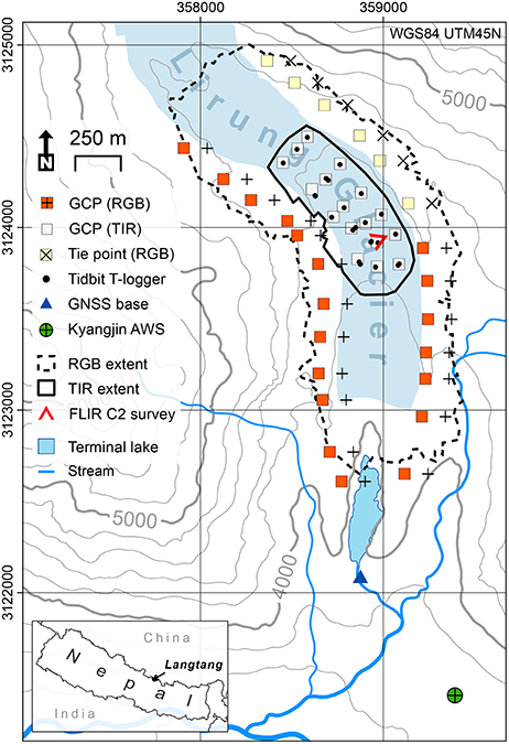
Figure 1. Study area at the debris-covered tongue of Lirung Glacier, Langtang Valley, Nepal. The map shows the locations of all ground control points (GCPs), tie points, Tidbit temperature loggers, the automatic weather station (AWS), and the FLIR C2 survey. The coverage of both the optical (RGB) and thermal infrared (TIR) surveys are also indicated on the map. The inset shows the location of Langtang Valley in Nepal.

3. Data and Methods

3.1. Temperature Measurements

Two main definitions of the temperature of a body can be distinguished (Becker and Li, 1995), which are both measured differently. First, there is the thermodynamic temperature of a body in thermal equilibrium, which can be measured by a thermometer for a given position in space. Second, there is radiometric temperature, which corresponds to the radiance emitted by a surface and is also referred to as skin temperature. It can be measured by a radiometer from a distance given that the emissivity of the body is known. In the case of homogeneous, isothermal bodies, the two temperatures agree. However, the situation is more complex for land surfaces with small-scale roughness and a composition of various materials, such as moist gravel, or sparse grass cover with exposed soil (Minnis and Khaiyer, 2000). This is particularly true under incoming solar radiation during daytime, which heats up the surface (skin) of a body and creates temperature gradients both within the body and at the body-air interface.

A temperature sensor placed on a surface will measure the micro climate surrounding the sensor, whereas a radiometer will measure the temperature emitted by the skin of the body (radiant temperature). Consequently, the two temperature measurements correspond best for shaded surfaces or liquids with a submersed thermometer. Measurements may differ for thermometers placed on sunlit surfaces or within a body with inhomogeneous temperatures (e.g., sand during day time), and for radiometric temperatures if the atmosphere between the radiometer and the radiance-emitting surface has a different temperature than the surface.

3.2. Outline of Methodology

To produce and evaluate the UAV-derived surface temperature maps of the debris-covered Lirung Glacier five main steps were performed:

1. On 30 April 2016, a UAV survey of the glacier was performed in which we collected optical imagery. On 1 May 2016, thermal data was collected on three separate UAV surveys over the course of the morning. The acquired imagery of both sensors were processed into orthomosaics.

2. A correction for emissivity was applied to orthomosaics of radiant temperature to obtain actual skin temperatures of the debris. For this, a spatially distributed emissivity map was produced using object-based image classification of the optical data.

3. UAV-measured skin temperatures were evaluated against (1) in situ temperature measurements taken at the time of the survey using a set of distributed temperature sensors (Tidbit T-loggers), and (2) skin temperatures obtained with a hand-held thermal camera for a single location on the glacier. Biases in the Tidbit T-logger measurements caused by the micro climate from direct shortwave radiation on the sensors were determined in an experimental setup and corrected.

4. The UAV temperature product and emissivity-corrected Landsat 8 data from comparable conditions were compared to determine differences between UAV and satellite approaches for obtaining surface temperature.

5. A statistical analysis was performed to assess the influence of solar insolation and local topography on the warming of the glacier surface, and to determine which part of the variability in the surface warming rate can be explained by other debris properties and surface processes.

In the following sections the details of each step are given. A flowchart that outlines our methodology is provided in Figure 2.

FIGURE 2

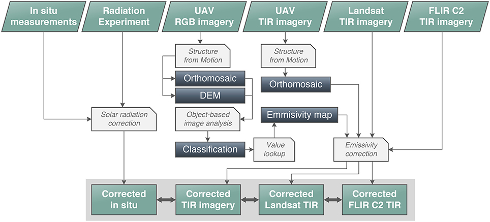
Figure 2. Flowchart that shows the steps used to process the spaceborne, airborne, and ground-based data into corrected output products.

3.3. Meteorology

Meteorological data from the nearby Kyangjin automatic weather station (AWS) located at 3,862 m.a.s.l (Figure 1) shows typical conditions for the time of the year for each of the surveys (Figure 3). Air temperature ranges from close to freezing at night to about 10℃ in the afternoon. After sunrise, temperatures rise very quickly because of the high incoming solar radiation found at this high elevation and sub-tropical latitude. The radiation data shows there were no clouds in the morning and that winds picked up around noon (Figure 3), which are both characteristic for the site. For the entire survey period there was no precipitation observed.

FIGURE 3

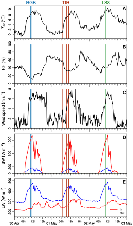
Figure 3. Meteorological data from the Kyangjin automatic weather station (Figure 1) for 30 April–2 May 2016. Panels (A–E) show the air temperature, relative humidity, wind speed, shortwave radiation, and longwave radiation, respectively. The vertical lines indicate the times of the RGB and TIR surveys performed with the UAV, and the time of the Landsat 8 overpass (Table 1).

3.4. UAV Surface Temperature

3.4.1. Optical Survey

On 30 April 2016 an approximately 2 km2 portion of the tongue of Lirung Glacier (Figure 1) was surveyed using a fixed-wing eBee from UAV manufacturer SenseFly. The UAV was launched from a point along the eastern moraine and was set to land in a meadow below. The eBee was equipped with a Sony WX RGB (i.e., red-green-blue) compact camera with an 18.2 megapixel sensor. The camera's shutter was electronically triggered by the UAV autopilot along a predefined flightpath. Zoom, exposure and other camera settings were all controlled by the flight management software provided with the eBee, i.e., eMotion2 (SenseFly, 2017a). Two separate flights during clear skies and light winds were required to cover the entire survey area (Table 1). The UAV was set to adapt its flight altitude to the (general) topography and capture 6 cm resolution imagery, which roughly equates to a flight altitude of 210 m above the surface. Image overlap was set to 60% laterally and 70% longitudinally with respect to the flight direction. A total of 237 RGB images were captured by the camera. Flight paths and image locations of the two flights are provided as Supplementary Data.

TABLE 1

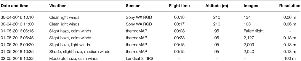
Table 1. Details of the optical and thermal UAV surveys, as well as the Landsat 8 thermal scene.

3.4.2. Thermal Infrared Survey

A ~0.4 km2 portion of the debris-covered tongue of Lirung Glacier (Figure 1) was monitored using the eBee mounted with a thermoMAP thermal infrared camera (SenseFly, 2017b). The uncooled microbolometer sensor of the thermoMAP has a relatively high resolution of 640 × 512 pixels and can measure surface temperatures between −40 and 160℃. Temperature resolution of the sensor is 0.1℃ and it performs automatic temperature calibration in flight based on the sensor's internal temperature. The thermoMAP assumes an emissivity of the surveyed surface of 1, and thus captures images of radiant temperatures only. The peak spectral response of the sensor lies at 10 μm, with a full width half maximum of approximately 5 μm (8.5–13.5 μm) (SenseFly, 2017b). The camera stores its imagery in uncompressed TIFF. We surveyed a considerably smaller area than for the optical flights because the higher energy consumption of the sensor. Moreover, on the contrary to optical UAV surveys, multi-flight surveys of the glacier are infeasible with a thermal camera due to rapidly changing surface temperature conditions between flights. Off- and on-glacier terrain could not be surveyed synchronously because of the low flight altitude that is required for proper functioning of the thermoMAP (<120 m from the surface) and the high lateral moraines of the glacier (up to 100 m).

The UAV was deployed over the survey area four times over the course of the morning on 1 May 2016 (Table 1) to acquire a spatio-temporal signature of the surface temperature. A first flight was performed early morning before sunrise at 6:15, but the UAV lost radio contact and returned without usable imagery. Subsequent successful flights of approximately 15 min each were performed at 6:45, 9:20, and 10:35, which together collected 6,176 highly-overlapping thermal images. These flights will be referred to as Flight 1–3 hereafter. During Flight 1 there was little to no incoming shortwave radiation (Figure 3), and most of the surveyed surface was still in the shade, except for the western moraine. Flight 2 was performed during fully sunlit conditions and an incoming shortwave radiation of approximately 600 W m-2. By Flight 3, air temperatures and incoming shortwave radiation had increased to 8℃ and 900 W m-2, respectively (Figure 3). However, during the third flight there was intermittent blockage of the sun by thin, local clouds. Flight paths and image locations of Flight 1–3 are provided as Supplementary Data.

3.4.3. Ground Control Survey and Processing

The eBee records coordinates for every image it takes using its GPS module with an accuracy of about 5 m. However, to georeference and co-register the high-resolution surveys performed with the UAV, ground control surveys are required. Accurate measurement of the coordinates of markers that will be visible on the captured imagery (e.g., Westoby et al., 2012; Lucieer et al., 2013) yields ground control points (GCPs) that can be utilized in the image processing.

In this study we have deployed two different types of markers near or on Lirung Glacier. Prior to the optical survey on 30 April a total of 20 rectangular pieces red fabric of approximately 1.0 × 1.2 m were distributed over the lateral moraines of Lirung Glacier (Figure 1). The planned ground control survey on the eastern moraine of the glacier was not fully completed due to time constraints imposed by changing weather conditions. For the parts of the moraine where the survey could not be completed six virtual ground control points, or tie points (Figure 1), were determined using georeferenced UAV imagery that was acquired in October 2015, using techniques similar to those described in Immerzeel W. et al. (2014).

For the survey with the thermal camera markers of different material were required, since the striking contrast in visible light between the red fabric and the surrounding terrain is not captured in the thermal infrared part of the spectrum. Markers are required with sufficient contrast in the radiant temperature that is captured by the thermoMAP sensor. The relation between radiant temperature and surface temperature is controlled by emissivity and incoming longwave radiation (Li et al., 2013; Lillesand et al., 2015), and is given by Stefan-Boltzmann's law :

$\begin{array}{rc}{T}_{\mathrm{\text{s}}}=\sqrt[4]{\frac{\sigma T_{\mathrm{\text{rad}}}^4-(1-\epsilon ){\mathrm{\text{LW}}}_{\downarrow }}{\epsilon \sigma }}& (1)\end{array}$

where T_s is surface temperature (K), T_rad the radiant temperature (K), ε the emissivity, σ the Stefan-Boltzmann constant (5.67 × 10-8), and LW_↓ the incoming longwave radiation (W m-2). To obtain clear contrast on thermal imagery, it is therefore possible to use markers with considerably different emissivity than the surrounding natural surfaces on the glacier (~0.87–0.98). This was achieved by using 1.0 × 1.0 m corrugated plastic squares wrapped in aluminium foil. Aluminium has an emissivity of 0.03–0.07 (Lillesand et al., 2015) and will exhibit a low radiant temperature relative to surrounding natural surfaces.

The center position of each marker (latitude, longitude, and elevation) was measured with a Global Navigation Satellite System (GNSS); a base station and a rover that both consist of a Topcon GB1000 antenna with a PG-A1 receiver. The base station was set up at a fixed position near the outlet of the glacier (Figure 1) and was in operation during the entire ground control survey, which was performed on 29 and 30 April 2016. We used the system in post-processed kinematic mode and measured each marker for about 30 s. This particular system has a reported geodetic accuracy of about ~0.2 m in x, y, and z (Wagnon et al., 2013). The measured points were post-processed in Topcon Tools (Topcon Positioning Systems, 2009) and placed accurately in a real-world coordinate system through a precise point positioning procedure (Zumberge et al., 1997) to acquire the final GCP positions.

3.4.4. Optical Imagery Processing

Imagery acquired in the optical UAV survey was processed into image mosaics using the Structure from Motion with Multi-view Stereo (SfM-MVS) algorithm (Triggs et al., 2007; Snavely et al., 2008; Szeliski, 2011; Lucieer et al., 2013; Immerzeel W. et al., 2014; Carrivick et al., 2016) implemented in Agisoft Photoscan Professional 1.2.6 (Agisoft LLC, 2016). In this procedure, feature recognition and matching algorithms (Szeliski, 2011) are applied to the overlapping imagery to generate high-resolution 3D point clouds of the glacier, which are accurately georeferenced using the GCP coordinate information. The 3D-information from the point clouds was used to stitch the imagery and apply orthorectification, i.e., correction of image distortion and parallax caused by topographical variations and varying viewing angles of the UAV, and create an orthomosaic. The SfM-MVS procedure followed here is similar to as described in Kraaijenbrink P.D.A. et al. (2016). The optical orthomosaic was exported at 0.1 m resolution and the point cloud was gridded into a 0.2 m resolution DEM.

The aluminum thermal markers were clearly identifiable both in the thermal imagery (squares consistently below -10 °C) and optical imagery (distinctly bright squares). To improve spatial co-registration of the optical image products with the thermal data, the GCPs designed for the thermal surveys were also used to process the optical imagery. The use of thermal GCPs, which are focused in the thermal survey area, ensures a high horizontal accuracy in the area where it is required.

3.4.5. Thermal Imagery Processing

To process each of the three successful thermal surveys we used Postflight Terra 3D (version 4.0.104), which is SfM-MVS processing software provided by senseFly with the eBee (SenseFly, 2017a). It is a licensed derivative of the commercial SfM-MVS software suite Pix4D Mapper Pro (Pix4D SA, 2017). Although Photoscan is the most commonly used SfM-MVS software in geoscience applications (e.g., Lucieer et al., 2013; Immerzeel W. et al., 2014; Turner et al., 2014; Ryan et al., 2015; Kraaijenbrink P. et al., 2016; Kraaijenbrink P.D.A. et al., 2016; Mallalieu et al., 2017; Ryan et al., 2017; Watson et al., 2017), and it has also been proven to work with thermal imagery (Turner et al., 2014), we chose to use Postflight because of its seamless integration with the thermoMAP camera (SenseFly, 2017a).

For each of the flights, all available images were used as input in a photo alignment procedure in Postflight. This procedure generates an initial point cloud and determines the orientation of the camera for each photo. Equal to SfM-MVS processing of optical imagery, feature recognition algorithms were applied to match similar points on multiple images. Visual pre-selection of images based on quality was not performed because the quality of the raw thermal imagery is difficult to judge and because of the large number of images per flight. To achieve optimal output, we ran the alignment procedure on the full resolution images and used a high image tie point limit. Nevertheless, many of the images were discarded by the software in this first processing step for all three flights, because insufficient tie points were found on certain image pairs. This is most likely due to the relatively low contrast of the thermal imagery for the debris-covered glacier surface. For Flight 1–3 a total of 800, 769, and 759 images (out of 2,127, 2,007, and 2,038) were maintained by Postflight for further processing, respectively.

Georeferencing of the thermal imagery was achieved by matching all available thermal GCPs (Figure 1) visually on all the aligned images they appeared on. The markers were pinpointed visually in Postflight's raycloud editor. The number of images to which a single GCP was matched ranged from 14 to 96. After the GCP matching, a point cloud densification was performed on highest accuracy settings to create a thermal 3D model of the glacier surface. The model was then gridded into an orthomosaic raster with a resolution of 0.3 m.

3.4.6. Image Co-registration

Usage of the thermal GCPs in the SfM-MVS processing of both the optical and thermal UAV imagery provides good geodetic accuracy of the datasets. However, small spatial displacements on the order of a few decimeters between all four orthomosaics remain. To reduce those, the data were shifted horizontally using the mean displacement of the imagery at the thermal markers with the GNSS-measured coordinates, which was determined visually in a geographical information system. This provides a spatial match between the optical and thermal UAV products that is sufficiently accurate for emissivity correction of the thermal data. Implementation of co-registration algorithms for multi-sensor imagery layers (Turner et al., 2014) can potentially provide a better match and improved multi-band image analysis capabilities, but this is beyond the scope of and requirements for this study. The accuracy of the eventual co-registration was determined separately for each pair of orthomosaics from the displacements between the images at the thermal markers, and error statistics were derived from this data.

3.4.7. Object-Based Emissivity Correction

To obtain surface temperature maps from the radiant temperature orthomosaics an emissivity correction must be applied (Li et al., 2013) using Equation (1). The debris-covered surface of Lirung Glacier is spatially heterogeneous and within the thermal survey area there are large boulders, gravel, sand, patches with dry shrubs, supraglacial ponds, and ice cliffs. The geology and consequently the supraglacial debris in this part of the valley largely consists of gneiss and quartzite (Kohn et al., 2005). Since all these surfaces have different emissivities, spatially distributed emissivity data is required to derive an accurate surface temperature. Such data could be acquired using in situ measurements of emissivity, generally performed with the box method (Sobrino and Caselles, 1993) or variants thereof (Rubio et al., 1997). However, such measurements are time and energy consuming, and as a result not feasible during the field campaigns in our remote study area. Therefore, we chose to estimate spatially distributed emissivity through image classification of the optical orthomosaic with object-based image analysis (OBIA) and the use of emissivity values (debris: 0.94, dry vegetation: 0.87, rough ice: 0.97, water: 0.98) reported in literature (Salisbury and D'Aria, 1992; Lillesand et al., 2015).

OBIA is a classification method that is preferred over traditional pixel-based image analysis methods when the objects of interest are multiple pixels in size (Blaschke et al., 2014). The OBIA procedure consists of two main steps. First, imagery is segmented into objects, i.e., groups of pixels that are spectrally homogeneous or that are part of a shape (Trimble, 2017). Second, the generated objects are classified based on specific object features. These can be spectral statistics of the pixels of which the object consists, but also object neighbor relations and object shape (Blaschke et al., 2014).

Our OBIA procedure is performed entirely in eCognition Developer 9.3 (Trimble, 2017). Input for the procedure are the optical orthomosaic and the DEM-derived slope. Both products were resampled to 0.2 m to match resolution. A single segmentation procedure was performed generating a single object level, purely based on the three-band optical orthomosaic. To accurately capture small patches of vegetation, small supraglacial ponds and exposed ice cliffs, the scale of the output objects was chosen to be moderately small with respect to the image resolution, i.e., an eCognition scale parameter setting of 25 (Trimble, 2017). For the actual classification of the objects a two-step approach was implemented. First, we chose to classify water and ice cliff objects visually, since accurate classification of these surface features requires sufficient training data (Kraaijenbrink P.D.A. et al., 2016) and there are only two relatively small ice cliffs with adjacent ponds in the thermal survey area. Second, to distinguish between vegetation and debris a nearest neighbor classifier was implemented in eCognition (Kraaijenbrink P.D.A. et al., 2016; Trimble, 2017). For each class, a training set of 15 samples was selected randomly. The classifier was subsequently applied using the five object characteristics that provided the largest class separability within the training set: blue band mean, red band standard deviation, green band standard deviation, brightness range, and mean slope. By evaluating the classification visually at 100 random points for each class, the classification's producer accuracy, user accuracy and kappa coefficient (Lillesand et al., 2015) were found to be 91.3, 94.0, and 0.85%, respectively.

To correct for emissivity through Equation (1), in situ observations of LW_↓ were used. During the surveys we measured LW_↓ only at the Kyangjin AWS. However, meteorological data from previous years (Steiner et al., 2015; Buri et al., 2016b; Steiner and Pellicciotti, 2016) and from recent field campaigns reveal that it is higher over the debris-covered surface of Lirung Glacier than at Kyangjin AWS due to longwave radiation emitted and reflected by surrounding steep headwalls, lateral moraine slopes, and debris mounds. Comparison of on- and off-glacier LW_↓ data from multiple fields campaigns reveals an approximate additional 20 W m-2, which we used to offset the Kyangjin AWS LW_↓ data.

To estimate the effect of uncertainty in emissivity on the derived surface temperatures we have applied a Monte Carlo sensitivity analysis. An ensemble of 1,000 random emissivity samples per surface type was drawn from a truncated normal distribution (0 ≤ ε ≤ 1) using a different mean and standard deviation for each surface type [debris: 0.94±0.015, dry vegetation: 0.87±0.062, rough ice: 0.97±0.012, water: 0.98±0.005, (mean ± sd)]. These were derived from sets of emissivities for metamorphic rock, vegetation, rough ice and sediment-laden water (Salisbury and D'Aria, 1992). For each ensemble member surface temperatures were calculated for each of the three thermal flights and ensemble statistics were derived.

3.4.8. ThermoMAP Bias Correction

Surface temperatures derived from the thermoMAP sensor have a remaining dark current bias that is due to the internal mechanics and calculations of the camera. The thermal response measured by an uncooled microbolometer sensor, such as from the thermoMAP, must be corrected with the internal sensor temperature (Ribeiro-Gomes et al., 2017), and this is performed automatically in flight. The temperature is estimated at the beginning of each flight leg (for each of the flights n = 24) by measuring the camera's shutter with the sensor, and comparing this with an internal thermometer (SenseFly, 2017b). However, if the internal temperature differs greatly from 20℃ large deviations can start to occur, especially on long flight legs (pers. comm. senseFly representative M. Montevecchio). Such a sensor bias is likely to be the case for our study (relatively short flight legs, but air temperatures of 0–8℃ at Kyangjin AWS). In our case, the potential biasing influence of the atmospheric column between the sensor and the ground on the measured temperature (Li et al., 2013; Torres-Rua, 2017) is likely limited due to the dry conditions, thin air and low flight height.

To remove the sensor bias it is required to know the skin temperature and emissivity of an object that was captured in the imagery at the time of the survey. Due to the lack of dedicated markers in our case, we assume that exposed clean ice is at the melting point of snow and ice (0℃) during Flights 2 and 3, and use the mean difference between the emissivity-corrected surface temperatures of a vertical clean ice band of one of the ice cliffs to calculate the sensor bias. The resulting sensor bias has subsequently been removed from all three thermal orthomosaics to obtain the final thermal imagery product. Note that this approach assumes that the bias is constant over the range of measured temperature values, which is most likely not the case. The required data to estimate the non-linearity of the bias is however unavailable.

3.5. In situ Temperature Measurements

3.5.1. Sensor Placement

A total of 25 HOBO TidbiT v2 temperature loggers with an accuracy of ±0.2 ℃ (hereafter referred to as Tidbits) were distributed on the surface of Lirung Glacier to validate surface temperature estimates from the thermal UAV survey. The sensors were placed in a semi-regular grid (Figure 1) on different surface types (Figure 4). Two Tidbits were submerged 5 cm in the water of a supraglacial pond underneath a float of semi-rigid foam. Most sensors received direct solar radiation for almost the entire day, but three Tidbits were placed into the shade to shield them from solar radiation. All sensors were operational during the aerial surveys and set to record temperature at a 5-min interval.

FIGURE 4

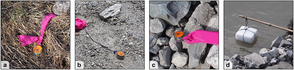
Figure 4. Different types of surfaces on Lirung Glacier the temperature loggers were placed on or in: vegetation (a), fine debris (b), coarse debris (c), and water (d). The pink ribbons were attached to the Tidbits to improve their discoverability.

3.5.2. Correction for Solar Radiation

Tidbit temperatures are overestimated when exposed to direct solar radiation due to the micro climate generated. To correct for this, we ran reference experiments at two AWS sites, one in Kathmandu and one in Langtang Valley. The Tidbit temperature measurements (T_tid) were compared with surface temperature (T_s) as derived from incoming and outgoing longwave radiation (LW_↓ and LW_↑) that was measured with radiometers (Apogee SI-111 and Kipp & Zonen CNR4), and using:

$\begin{array}{rc}{T}_{\mathrm{\text{s}}}=\sqrt[4]{\frac{{\mathrm{\text{LW}}}_{\uparrow }-(1-\epsilon ){\mathrm{\text{LW}}}_{\downarrow }}{\epsilon \sigma }}& (2)\end{array}$

Two types of surfaces were examined below the AWSs. Debris was artificially set up in the experiment that was run in Kathmandu, while naturally occurring dry vegetation was monitored at the Kyangjin AWS in Langtang Valley (Figure 1). The artificial debris layer comprised of a mixture of irregularly shaped concrete blocks, natural rocks and mud, which had a size distribution representative for supraglacial debris and comparable emissivity, as concrete has an emissivity of 0.92–0.94 (Lillesand et al., 2015). For practical reasons, the thickness of the layer was shallower (5–10 cm) than what is usually found on Lirung Glacier, but it was thick enough to completely cover the concrete substrate. For each surface type, ε was first set as the value minimizing the difference between T_s and T_tid (ΔT), using night-time data only. As ΔT increases with incoming shortwave radiation (SW_↓), separate regressions for each surface type were calculated using daytime observations where SW_↓>20 W m⁻²

$\begin{array}{rc}{T}_{\mathrm{\text{cor}}}=T_{\mathrm{\text{tid}}}-a{\mathrm{\text{SW}}}_{\downarrow }& (3)\end{array}$

where T_cor is the corrected Tidbit temperature and a the correction factor (K m2 W-1). It is assumed that with little or no direct shortwave radiation, i.e., at night, T_s and T_tid are equal, and so the regression was forced through the origin. Additionally, since all our thermal UAV flights performed between 6:45 and 10:50, Equation (3) only considers experimental observations collected before noon, which limits the influence of temperature hysteresis caused by Tidbit lag. Correction factors for the most suitable surface type were applied to the in situ temperature measurements for the Lirung thermal surveys. Corrections were not applied to Tidbits that were put in the shade or submerged in water, since these were not subjected to direct shortwave radiation.

SW_↓ varies considerably spatially over the hummocky debris-covered surface of Lirung Glacier because of varying aspects and shading effects that result from the small-scale surface topography. To account for this in the correction, we modeled distributed SW_↓ using the hemispherical viewshed algorithm of Fu and Rich (1999) and a 30 cm resolution resampled DEM derived from the optical UAV data. In the model, we used an effective atmospheric transmissivity of 0.42, which was determined by minimization of modeled and measured SW_↓ at the Kyangjin AWS (Figure 3). Any residual variability captured by the AWS as compared to the idealized modeled SW_↓ was superimposed on the modeled data.

3.6. Ground-Based Thermal Imaging

To compare the UAV surface temperature measurements with independent radiometric measurement, we have used a FLIR C2 (hereafter C2) compact hand-held thermal camera during the UAV flights. The camera has a 80 × 60 pixel uncooled microbolometer TIR sensor and a 640 × 480 pixel optical sensor that take aligned images synchronously. The TIR sensor senses objects of −10 to 150 °C in the in the 7.5–14 μm range, with a thermal sensitivity of 0.1 °C. The accuracy of the sensor is ±2 °C at an outside temperature of 25 °C (FLIR Systems, 2017).

The C2 survey was performed at a single location during the entire survey (Figure 1). The camera was mounted on a monopod that was fixed between debris, facing in west-southwest direction at the largest largest ice cliff within the survey area. In the field of view of the camera most of the ice cliff was visible, as well as parts of the adjacent supraglacial pond and the surrounding debris. The shutter of the C2 was manually triggered at a semi-regular interval of 10 min between 06:40 and 11:09.

Radiometric thermal data and the optical images taken by the camera's sensors were retrieved using FLIR's ResearchIR software. As a result of the relatively unstable monopod setup and the manual triggering of the shutter, the captured imagery for the different time steps was not perfectly coregistered. To coregister the data accurately, manual tie points were identified on the optical imagery in a geographical information system, which were subsequently applied to both the optical and thermal image sets. From the optical imagery, zones of different surface classes were identified visually corresponding to those of the classified UAV data, but with an extra distinction between clean and dirty ice. For each zone an emissivity correction was applied using Equation (1) and the values reported in section 3.4.7. For comparison of the data with UAV-derived T_s, zones that correspond spatially to those defined on the C2 imagery were identified visually on the UAV-derived orthomosaic.

3.7. Landsat 8 Thermal Infrared Comparison

Medium resolution thermal infrared satellite imagery [e.g., Landsat 7 (60 m) (Rounce and McKinney, 2014), ASTER (90 m) (Mihalcea et al., 2008a,b; Foster et al., 2012), and Landsat 8 (100 m) (Kraaijenbrink et al., 2017)] has been previously used to infer debris thickness using temperature inversion methods. To get an impression of the accuracy and spatial detail of such spaceborne thermal infrared imagery for analyses of the debris layer, we compared satellite and UAV-derived surface temperatures.

For the comparison, surface temperatures of Lirung Glacier's debris cover were estimated from Landsat 8 Thermal Infrared Sensor (TIRS) data. We used a Landsat 8 scene (LC81410402016123LGN00) that was acquired on 2 May 2016 at 10:32 local time (Table 1), one day after the thermal UAV survey. Although the original sensor resolution of the TIRS instrument is 100 m, the only data that is made available by the United States Geological Survey comprises thermal imagery that is coregistered, geometrically corrected and resampled using irreversible cubic convolution to match the 30 m resolution of the satellite's optical data (USGS, 2016). Uncertain weather conditions prevented us from performing the UAV and in situ measurements the same day as the Landsat 8 overpass, but atmospheric and meteorological conditions during the morning of both acquisition days were generally comparable (Figure 3). Nevertheless, comparison of absolute temperature values of the two different products is inaccurate because of three reasons: (1) a small amount of cloud cover was present during the final UAV flight, which was not the case at the time of the satellite acquisition; (2) we observed slightly more atmospheric haze on 2 May 2016, but we did not quantify changes in atmospheric transmissivity; (3) Landsat 8 TIRS is affected by stray light, which can result in considerable overestimations of the recorded radiance that are hard to correct (USGS, 2016). Comparison of spatial variability, on the other hand, is still meaningful.

Surface temperatures were determined from the satellite's band 10 by first calculating the top of atmosphere brightness temperature from the Level 1 satellite product using the standard procedure described by USGS (2016). A subsequent correction for emissivity was applied using Equation (1) and the UAV-derived emissivity map, resampled to the satellite product resolution. Comparison with the UAV-derived surface temperatures was performed by evaluating pixel statistics of the UAV thermal data for each Landsat pixel.

3.8. Surface Temperature and Topography

To evaluate the influence of the small scale hummocky topography of Lirung Glacier on debris surface temperatures, we have compared the mean warming rate over the entire morning (K h-1) with the modeled SW_↓ and four DEM derivatives: aspect, slope, flow accumulation and high pass filtered DEM (see next paragraph). For the analysis, we have fitted a random forest regression model with the warming rate as dependent variable and the five topography indicators as independent variables. A random forest is a statistical machine learning algorithm that can fit non-linear relations, is insensitive to overfitting, has no requirements on the statistical distribution of variables, and is largely insensitive to multicollinearity (Breiman, 2001). It is therefore particularly suitable for this analysis. The algorithm can also provide a natural measure of variable importance in model prediction as well as measures of total explained variance (Breiman, 2001; Louppe et al., 2013). These were used to determine to what extent solar insolation in combination with topography is causing temperature change, and how much is unexplained by different processes. The entire analysis was performed only for the actual glacier surface (Figure 6a), and using data resampled to 3 m (n = 33, 999) to reduce the required processing time for the random forest algorithm and to remove noise in both the surface temperature maps and the DEM.

Aspect is closely linked to SW_↓, since the amount of insolation at a point is directly related to the solar azimuth and the local aspect. However, on the contrary to SW_↓ it is not affected by the viewshed at a point. It can easily be calculated from a DEM and does not require data on surrounding topography, and is therefore of interest as a predictor of the warming rate. Slopes (facing toward the sun) are exposed more directly to the sun than flat areas and may be dryer, since water is expected to run off to lower areas. As a result, it could be that areas of relatively high slope have an increased warming rate due to increased radiation, decreased debris heat capacity, and less evaporative cooling. A flow accumulation map, or upstream area map, indicates the size of the catchment upstream of a pixel. The larger the upstream area, the higher the debris moisture content may be due to supraglacial runoff and the lower the warming rate. Note that supraglacial melt water runoff also depends strongly on the configuration of the englacial drainage network. A high-pass filtered DEM, here created for a large circular focal window of 25 m, provides information on relative local elevation. That is, whether a point is relatively high or low in comparision with it's surroundings. Local depressions can be expected to be more humid and cooler, whereas mounds and crests may be dryer and warmer.

4. Results

4.1. Tidbit Correction and Measurements

Radiometer-derived T_s (section 2) and T_tid showed considerable deviations for both reference experiments (Figure 5). Temperature differences between the two methods (ΔT) were as high as 10 ℃ over the course of the morning. The debris experiment performed in Kathmandu revealed a more linear relation between ΔT and SW_↓ than the vegetation experiment performed near the study area at the Kyangjin AWS. There is more hysteresis for the latter, which is most likely caused by evaporation of moisture from the vegetation and the top soil layers. The range of SW_↓ for the two experiments is considerably different because of the difference in altitude (~1,400 and ~4,000 m) and atmospheric pollution at the two reference sites. The regression analysis of ΔT against SW_↓ (section 3) resulted in correction factors a of 13.3 × 10⁻³ and 11.4 × 10⁻³ K m² W⁻¹ for debris and vegetation, respectively.

FIGURE 5

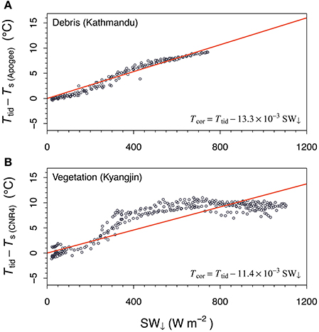
Figure 5. Difference between radiometer-derived and Tidbit-derived surface temperatures versus incoming shortwave radiation for daytime measurements before 12 a.m. The two panels show the biases for an experimental debris layer in Kathmandu (A) and natural vegetation present at below the Kyangjin AWS (B). The red lines show the linear regressions that were used for bias correction of the Tidbits.

The T_cor values for the morning of 1 May 2016 reveal a large range in temperatures between flights and between different surfaces (Table 2). During thermal Flight 1 (06:45), measured in situ temperatures were generally just below freezing point with little variability between different Tidbits. This is similar to air temperature observations at the Kyangjin AWS, which are just above freezing point but measured 250 m lower (Figure 3). As incoming radiation and temperature increase over the course of the morning, T_cor increases considerably with mean values up to 28 ℃ for vegetated surfaces. Water temperatures only changed slightly throughout the morning and shaded tidbits warm considerably slower than those in direct sunlight.

TABLE 2

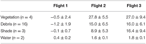
Table 2. Statistics of T_cor at the time of the thermal UAV flights for the four different surface types (mean ± sd).

4.2. Image Registration Accuracy

After SfM-MVS processing of the optical and thermal UAV surveys we co-registered the imagery by applying shift factors (x, y) for the optical survey (0.05, 0.03 m), thermal Flight 1 (0.18, -0.15 m), thermal Flight 2 (0.14, -0.16 m), and thermal Flight 3 (0.13, -0.15 m) to optimally match all orthomosaics with the GNSS-measured thermal GCPs. The root mean square errors (RMSE) at the thermal markers show a considerable improvement after application of the shift (Table 3). Before shifting, the thermal orthomosaics were already reasonably well registered with each other, despite completely independent processing of the three flights in Postflight. The horizontal shift between the optical and thermal orthomosaics may thus be caused largely by differences in processing and optimization algorithms between Photoscan (optical data) and Postflight (thermal data).

TABLE 3

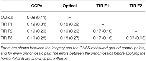
Table 3. Root mean square errors (m) of orthomosaic co-registration at the thermal markers locations (n = 17).

4.3. Image Classification and Emissivity

The result of the object-based image classification is shown in panel C of Figure 6. The most abundant surface type in the study area is debris with 92.3%, followed by vegetation (7.2%), ice cliff (0.3%), and water (0.2%). Vegetation is mainly present on the western lateral moraine, and not so much on the glacier surface itself. Using the classification and emissivity values reported in section 3.4.7, the emissivity map with mean emissivity of 0.93 was derived (Figure 6d).

FIGURE 6

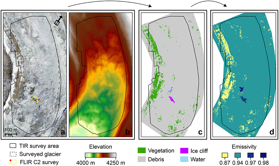
Figure 6. The input data used and the output data created in the emissivity estimation procedure: (a) the orthomosaic and (b) digital elevation model that follow from SfM-MVS processing of the optical UAV data; (c) the object-based image classification; and (d) the final emissivity map used to calculate surface temperatures.

4.4. Thermal Correction and Imagery

The three final thermal orthomosaics that were corrected for emissivity and sensor bias are shown in Figure 7. Due to the non-linear nature of Stefan-Boltzmann's law and the spatial distribution of emissivity, the emissivity correction is both spatially and temporally variable. Mean corrections that were applied to the imagery of Flights 1–3 were in the order of 0.5 ± 1.3℃, 0.8 ± 1.9℃, and 0.7 ± 1.9℃ (mean ± sd), respectively. The magnitude of mean sensor bias was determined to be 7.5℃ (7.6℃ for Flight 2 and 7.4℃ for Flight 3) from the ice cliff surface at melting point. The bias for the same ice cliff pixels for early morning Flight 1 is indeed less, i.e., 4.6℃, indicating that the ice surface was not yet at melting point at that time. For the bias correction the mean bias based on flight 2 and 3 was subtracted for all three flights.

FIGURE 7

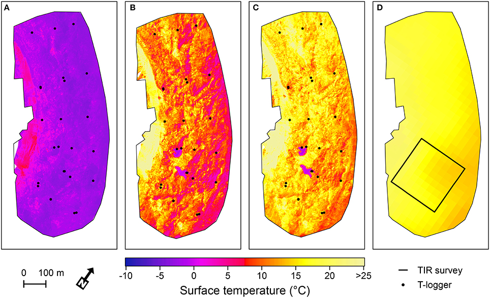
Figure 7. Emissivity and bias-corrected surface temperature orthomosaics of the three UAV flights on 1 May 2016 (A–C; 06:45, 09:20, and 10:35) and the brightness temperature of the Landsat 8 band 10 on 2 May 2016 at 10:32 (D). The black rectangle in (D) indicates the extent of Figure 10.

Similar to the in situ measurements of T_cor, the magnitude of UAV-derived T_s varies greatly over the morning, with temperatures for thermal Flights 1–3 (℃) of −1.4 ± 1.8, 11.0 ± 5.2, and 15.3 ± 4.7 (mean ± sd), 95th percentile ranges of −3.4 to 3.6, 4.0 to 25.7, and 8.6 to 27.5, and maxima of 9.1, 43.0, and 49.7, respectively (Table 4). It is clear that in the early morning the mostly shaded glacier surface has not yet warmed and surface temperatures have low spatial variability. Flight 2 shows a much warmer surface with high spatial variability. On the hummocky debris-covered surface of the glacier there are warm areas that received greater insolation, e.g., crests and slopes that face toward the azimuth of the rising sun, and colder parts in local depressions and north-facing slopes (Figure 7B). The last flight, with the debris exposed to greater and more evenly spatially distributed insolation under higher solar elevation angles, has overall high values of T_s that are less spatially variable (Figure 7C). For all three flights there is a distinct lateral trend in T_s that is directly related to the duration of insolation, with the western parts of the glacier being exposed by to the sun first. With respect to the different surface classes, debris and vegetation are warmer than ice and water for all three flights, as expected. Remarkably, vegetation is consistently warmer than debris for all flights. This is likely due to its higher abundance on the western moraine slope. Also worth noting is that ice is generally warmer than water, which could be due to the dark debris film on large parts of the ice cliffs.

TABLE 4

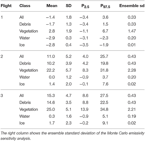
Table 4. Mean, standard deviation, 2.5 and 97.5 percentiles of T_s for the three UAV flights for the survey area and for each class.

The sensitivity of T_s for variations in emissivity of the surface classes is limited (Table 4). The standard deviations of raster average T_s for each Monte Carlo member in the ensemble (n = 1, 000) for F1–F3 are only 0.33, 0.43 and 0.43 ℃, respectively. The uncertainty in the surface temperature for vegetation only is considerably larger, as the emissivity of dry vegetation is more uncertain (section 3.4.7), emissivity is lower, and vegetation has the highest surface temperatures. Ice and water, on the other hand, have relatively certain and high emissivities as well as generally low temperatures, and consequently have low ensemble uncertainty.

4.5. Surface Temperature Comparison

Comparison of surface temperature derived from the Tidbits (T_cor) and from the UAV imagery (T_s) for each of the three thermal surveys and for all Tidbits showed that the recorded temperatures were largely in agreement (Figure 8A). The data scatter mainly around the 1:1 line and are generally the same order of magnitude (r = 0.93). The data of Flight 1 show the best agreement with a mean $T_{\mathrm{\text{cor}}}^{\mathrm{\text{F1}}}$ and $T_{\mathrm{\text{s}}}^{\mathrm{\text{F1}}}$ of −0.9 and −1.6℃, respectively, and a RMSE of 0.9℃. Note that of the three thermal flights, the Tidbit correction that was applied for this flight was minimal because of low SW_↓ in the early morning, and that the applied thermal sensor bias correction was independent of $T_{\mathrm{\text{s}}}^{\mathrm{\text{F1}}}$. The agreement between T_cor and T_s for Flight 2 is less, as there were considerable overestimations of surface temperature by $T_{\mathrm{\text{cor}}}^{\mathrm{\text{F2}}}$ of over 10℃ for some of the Tidbits. The RMSE for this flight was also considerably higher with 7.0℃. The last flight of the morning shows again better agreement with an RMSE of 5.1℃. Tidbits that were put on vegetation still have a considerable bias in this case, but especially those on debris show relatively good agreement with RMSE values of 7.8 and 3.7℃, respectively.

FIGURE 8

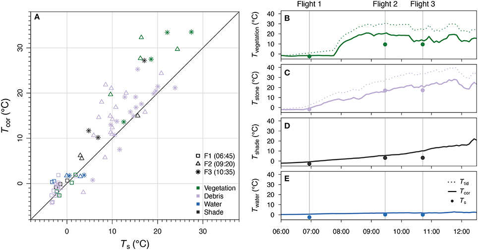
Figure 8. Corrected Tidbit temperature measurements (T_cor) against corrected surface temperatures from the three UAV flights (T_s) (A). Point shape denotes the UAV flight, point color the surface class, and the black line a 1:1 relation. (B–E) Show time series for selected Tidbits of the surface classes vegetation, debris, shade, and water, respectively. For vegetation and debris both the uncorrected (T_tid) and corrected temperatures (T_cor) are plotted. The points on (B–E) indicate T_s at the Tidbit location.

Time series of a selection of the Tidbits (Figures 8B–E) for each surface type that have a good match between T_cor and T_s show the variability in Tidbit temperature over the course of the morning. Tidbits in direct sunlight clearly had fluctuating temperature profiles, while measurements in the shade or in water are relatively stable and smooth over time. The temperature of Tidbits directly exposed to the sun deviate considerably from T_s, but temperature measurements in the shade and in water agree well. Therefore it is likely that the deviations between T_cor and T_s can be largely explained by errors in the Tidbit measurements.

4.6. Ground-Based Thermal Imagery

Time series with statistics for four zones of different surface type (Figure 9a) of the surface temperatures derived from the C2 imagery ($T_{\mathrm{\text{s}}}^{\mathrm{\text{C2}}}$) are shown in Figure 9e. Similar to T_cor and UAV-derived T_s, surface temperatures measured by the C2 are low in early morning at the start of the time series (−7.4 ± 0.7℃) and quickly rise as radiation increases. $T_{\mathrm{\text{s}}}^{\mathrm{\text{C2}}}$ for debris continues to rise steadily until 10:00 when it reaches 19.9 ± 3.7℃, while for ice it stabilizes relatively quickly to a temperature just below 0 °C, i.e., around the melting point of ice. Since the imagery thus has very low sensor bias, no bias correction was required. Only a slight difference between clean and dirty ice patches is present, as after 08:00 dirty ice has a mean temperature that is on average 0.2 °C above that of clean ice. On the C2 imagery, the temperature for the supraglacial pond (5.1 ± 3.8℃) rises to levels considerably above those of the ice, but remain well below that of debris. After 10:00 all zones exhibit a decrease in surface temperature of ~2.5 °C, which coincides with the thin local clouds that were observed during the last flight.

FIGURE 9

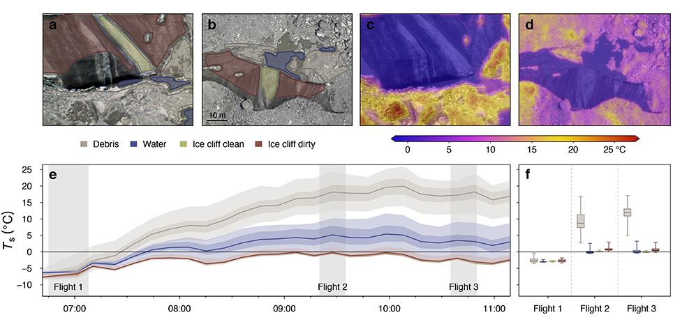
Figure 9. Ground-based FLIR C2 optical (a) and thermal infrared (c) imagery (09:28 example) of a selected ice cliff, supraglacial pond, and the surrounding debris location indicated in Figure 6a. UAV optical (b) and thermal infrared nadir orthomosaics (d) of the same location (Flight 2, 09:20–09:35). Image regions used for comparison of the two datasets are indicated by the polygons (a,b). Time series with region statistics (mean, interquartile range and 95th percentile range) of $T_{\mathrm{\text{s}}}^{\mathrm{\text{C2}}}$ are shown in (e), and boxplots of $T_{\mathrm{\text{s}}}^{\mathrm{\text{F1}}}$, $T_{\mathrm{\text{s}}}^{\mathrm{\text{F2}}}$ and $T_{\mathrm{\text{s}}}^{\mathrm{\text{F3}}}$ for the corresponding regions on the UAV imagery in (f).

Figure 9f shows boxplots of $T_{\mathrm{\text{s}}}^{\mathrm{\text{F1}}}$, $T_{\mathrm{\text{s}}}^{\mathrm{\text{F2}}}$ (Figure 9c) and $T_{\mathrm{\text{s}}}^{\mathrm{\text{F3}}}$ for the zones corresponding to Figures 9a,b. Compared to early morning $T_{\mathrm{\text{s}}}^{\mathrm{\text{C2}}}$, $T_{\mathrm{\text{s}}}^{\mathrm{\text{F1}}}$ appears to be considerably higher with temperatures of −2.7 ± 0.4℃. Note, however, that over the course of Flight 1 $T_{\mathrm{\text{s}}}^{\mathrm{\text{C2}}}$ rapidly changes with a warming of about 5 °C, and that the C2-measured temperature right after the flight at 07:10 is more comparable (−3.5 ± 1.7℃). Contrastingly, temperature is 8 °C lower than $T_{\mathrm{\text{s}}}^{\mathrm{\text{C2}}}$ in the late morning, with a $T_{\mathrm{\text{s}}}^{\mathrm{\text{F3}}}$ of 11.9 ± 1.8 ℃ for debris. Supraglacial pond temperatures measured by the UAV as well as by the Tidbits (Figure 8E) are consistently near freezing and lower than $T_{\mathrm{\text{s}}}^{\mathrm{\text{C2}}}$.

4.7. Landsat vs. UAV

The Landsat 8 (L8) thermal imagery of 2 May 2016 that was processed into a surface temperature map ($T_{\mathrm{\text{s}}}^{\mathrm{\text{L8}}}$) shows that the satellite image failed to capture any substantial spatial variation over the area of interest (Figure 7). The pixel size of 30 m of the Landsat 8 thermal data, which is created by cubic convolution of the 100 m raw product (USGS, 2016), results in substantial smoothing and loss of detail as compared to the data obtained from the UAV. The raw data product is unavailable unfortunately. While $T_{\mathrm{\text{s}}}^{\mathrm{\text{F3}}}$ had a total range of about 50℃, a mean of 15.3 and standard deviation of 4.7, $T_{\mathrm{\text{s}}}^{\mathrm{\text{L8}}}$ only ranges between 18.2 and 27.3 °C, with a mean of 22.0 °C and a standard deviation of 2.1 °C. The overall spatial pattern of $T_{\mathrm{\text{s}}}^{\mathrm{\text{L8}}}$, however, appears to match the pattern of $T_{\mathrm{\text{s}}}^{\mathrm{\text{F3}}}$, with generally higher temperatures on the western side of the glacier.

A more detailed view on both the UAV and Landsat data is presented in Figure 10, where the same spatial subset of 240 × 240 m is shown for both datasets. Here it is further evidenced that the satellite image cannot capture the heterogeneity of T_s over a debris-covered glacier, and that moderate scale features with distinctly low temperatures such as ice cliffs and supraglacial ponds appear to have little to no effect on the temperature recorded by the satellite. Figure 10c shows a scatter plot of $T_{\mathrm{\text{s}}}^{\mathrm{\text{L8}}}$ against $T_{\mathrm{\text{s}}}^{\mathrm{\text{F3}}}$ for each Landsat pixel over thermal survey area. Although there is a significant correlation between the two products (r = 0.79), T_s found by the two different sensors is considerably different, with a mean overestimation of $T_{\mathrm{\text{s}}}^{\mathrm{\text{L8}}}$ of 6.9℃. This may partly be attributed to actual differences in surface temperature between the two days of acquisition, since there were differences in T_air and SW_↓ (Figure 3), and to differences in atmospheric transmissivity. The overestimation of radiance at the sensor caused by stray light is also likely to play a role, as it may result in biases of up to 5 °C for band 10 (USGS, 2016). Standard deviations of $T_{\mathrm{\text{s}}}^{\mathrm{\text{F3}}}$ within each Landsat pixel (Figure 10c) show there is a very large variation in the relatively small 30 m plots of debris-covered glacier surface.

FIGURE 10

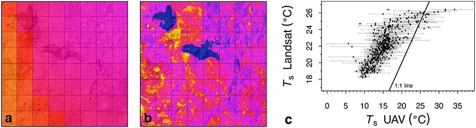
Figure 10. Comparison of a subset (extent denoted in Figure 7d) of T_s derived from Landsat 8 TIRS band 10 (2 May 2016 10:32; a) and from the thermal UAV survey (Flight 3, 1 May 2016 10:35; b). The grid overlay denotes the 30 m grid in which the Landsat data is provided. Panel (c) shows, for the entire extent of the UAV survey, a plot of Landsat pixel values against mean UAV surface temperatures within those pixels. The whiskers denote ±1 sd of the UAV surface temperatures.

4.8. Topography and Surface Temperature

The results of the random forest analysis that was used to evaluate the relation between topography and surface warming rate are presented in Figure 11. Of the five DEM derivatives that were analyzed there were only two that showed a clear relation: asp ect and SW_↓. Pixels with an east-facing aspect (45–135°) warm significantly more (+1.0 K h-1) than west-facing pixels (225–315°) (Figure 11g), a logical result as morning flights are analyzed. North-facing (315–45°) and south-facing (135–225°) pixels do show a difference in warming rate, but only very moderately with 0.1 K h-1. A more distinct effect on surface warming is caused by SW_↓, although the variable also exhibits considerable residual variability (Figure 11k). Linear regression revealed that SW_↓ alone explains 29.4% of the variance in the warming rate. The slope, upstream area and local relative elevation are all shown to have very limited influence on the warming rate (Figure 11l). In total, the combination of all independent variables can account for 38.8% of the variance.

FIGURE 11

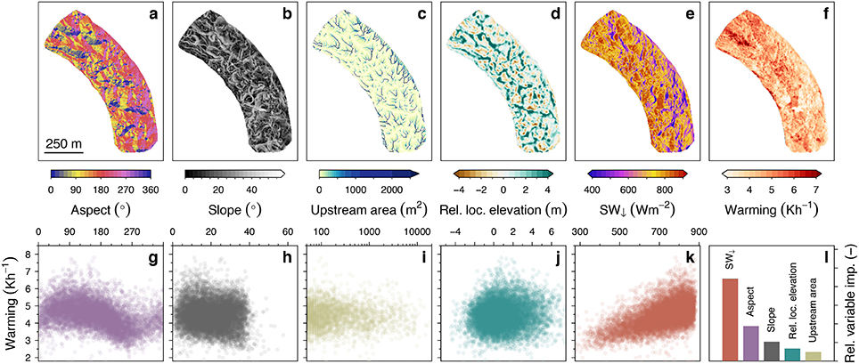
Figure 11. Comparison of the average warming rate (f) over the surveyed glacier surface area (Figure 6a) with five different DEM derivatives: aspect (a,g), slope (b,h), upstream area (c,i), relative local elevation (d,j), and mean incoming shortwave radiation (e,k). The relative importance of each variable as a predictor in a random forest regression is shown in (l).

5. Discussion

5.1. Applications of Thermal UAV Imagery

The methods employed in this study reveal the possibility of capturing spatially distributed T_s on a debris-covered glacier with unprecedented detail using a UAV equipped with a thermal infrared sensor. There are distinct spatial patterns in the output maps of T_s and the temporal variability of temperature is captured well in the three flights that were performed. The spatial variability in temperatures is partly explained by the complex local topography, as sunlit slopes and big boulders will warm more than shaded slopes and local depressions, and by differences in ground cover. The random forest analysis performed in this study shows that, of topography-related variables, incoming shortwave radiation has the largest effect on the warming rate of the glacier surface. In general, however, surface topography is unable to account for the majority of the warming rate signal, as 61.2% of the variance remains unexplained. Consequently, spatial variations in the glacier's surface properties and processes seemingly play a large role in controlling debris surface temperatures. The high-resolution thermal imagery therefore has various potential applications in the research of the debris-covered glaciers.

An obvious application of high-resolution thermal imagery is to inversely estimate debris-cover thickness (Mihalcea et al., 2008b; Foster et al., 2012; Rounce and McKinney, 2014; Schauwecker et al., 2015; Gibson et al., 2017; Kraaijenbrink et al., 2017), since thickness is an important variable in the surface energy balance of debris-covered glaciers (e.g., Nicholson and Benn, 2006, 2013; Collier et al., 2015; Ragettli et al., 2016). As we show in this study, the UAV is able to capture spatial patterns and heterogeneity in T_s (Figures 7, 10). This would allow for detailed estimations of debris thickness, which in turn may lead an improved understanding of small-scale glacio-hydrological surface processes on debris-covered glaciers. The temporal information on T_s provided by the repeat UAV surveys might be particularly valuable. Analysis of spatially variable warming rates of the debris (such as presented in Figure 11), for example, may provide more detail on actual debris thickness than a single image. Performing more flights over the course of the day and increasing the temporal resolution would therefore be worthwhile.

Secondly, surface temperature imagery at such high resolution may reveal important insights in the energy balance of a debris-covered glacier. The energy balance drives the melt of the debris-covered tongues and several studies point toward a yet unexplained faster surface lowering of the tongues of these glaciers than what can be expected based on the melt suppression by thick debris (Kääb et al., 2012; Gardelle et al., 2013; Pellicciotti et al., 2015; Azam et al., 2018). It is unclear whether this behavior can be attributed to turbulent fluxes, supra-glacial features such as cliffs and ponds, a reduced emergence velocity or other processes (Vincent et al., 2016; Azam et al., 2018). Highly detailed information about the surface temperature provides LW_↑, a term often assumed to be spatially constant and only measured point-scale at a weather station (Reid et al., 2012; Steiner and Pellicciotti, 2016). Our results show it is highly variable and will therefore also explain a large part of the variability in net energy available for melt. In addition, the surface temperature controls the sensible heat flux, which plays an important role in the energy balance of debris-covered glaciers and ice cliffs (Steiner et al., 2015; Buri et al., 2016a,b; Steiner and Pellicciotti, 2016). A comparison of thermal imagery collected before and after precipitation events might also help identify the role of moisture in the debris layer and its effect on latent heat fluxes, and lead to an overall improvement in turbulent flux parameterizations (e.g., Radić et al., 2017).

Thirdly, thermal UAV imagery could be applied in understanding the surface and subsurface hydrology. Englacial hydrology likely plays a key role in the drainage and transport of melt water through the glacier to the outlet (Miles et al., 2017), but the drainage paths are complex and difficult to measure. With a combination of thermal imagery, optical imagery, and the high-resolution DEM, it may be possible to infer supraglacial (sub-debris) and englacial drainage patterns.

5.2. Satellite-Based Surface Temperatures

Spaceborne thermal infrared imagery has the advantage that, if atmospheric conditions permit, T_s can be acquired relatively accurately for large spatial extents and remote areas (Li et al., 2013). Currently, this is a limitation of UAVs, since it is infeasible to deploy them over large inaccessible areas on a regular basis. However, in the study of supraglacial debris, the distinct advantages of thermal satellite imagery are largely counteracted by the inability of its moderate resolution to resolve the spatial heterogeneity in T_s found over debris-covered glaciers (Figure 10). Although the imagery can be used for coarse maps of debris thickness (e.g., Mihalcea et al., 2008b; Kraaijenbrink et al., 2017), surface melt varies considerably over smaller spatial scales, as indicated by the hummocky surface of most debris-covered glaciers. The heterogeneity of surface elevation changes (Immerzeel W. et al., 2014) and the thermal UAV data presented in this study further supports a high variability of melt rates and possibly debris thickness. To better understand the local surface energy balance and the processes involved, thermal imagery with a sufficiently high resolution, i.e., a resolution finer than the spatial scale of the melt patterns, is required. An additional advantage of the UAV is the possibility to deploy it synchronously with other in situ measurements to acquire complementary data.

In addition to the limitations imposed by sensor resolution, spaceborne thermal imagery is unable to capture sub-daily temporal variations in surface temperature (with the exception of very coarse-resolution geostationary meteorological satellites). The temporal variation observed in T_s over the three UAV flights, shows us that the use of a single satellite image in the assessment of the debris-layer could be an issue. Surface temperatures on debris-covered glaciers will vary significantly with day of year, time of day, and cloud conditions prior to acquisition, and the variability that occurs on short time scales (Figures 8B–E) will affect satellite-based analyses of the debris layer.

However, further implementation of the method we present in this study in the research of debris-covered glaciers does not only have the potential to improve our knowledge of small scale debris-covered glacier surface processes. Together with more process-oriented studies, more elaborate comparison of satellite and UAV data has the potential to improve the moderate resolution spaceborne thermal products, spatially and temporally. Namely, development of optical- or DEM-based downscaling of spaceborne thermal data using the UAV products could provide a way to upscale our knowledge on small scale surface processes to the glacier or catchment scale, which will enable better assessments of the impacts future changes in debris-covered glacier dynamics may have. Moreover, UAV data could prove valuable in the validation of thermal satellite imagery of debris-covered glaciers.

5.3. Bias Correction and Errors

The presence of the sensor bias of 6.9 °C reveals difficulties in the determination of absolute debris temperatures with the thermoMAP. The sensor bias correction we have applied is based on the assumption that clean ice cliff surfaces will be at melting point and thus 0 °C during Flight 2 and 3. This is a reasonable assumption, but admittedly there are uncertainties regarding its usability. For instance, atmospheric variability, such as air temperature and water vapor content, may affect the bias over time (Torres-Rua, 2017). It was not taken into account because of a lack of accurate data of the atmospheric column over the glacier that is required for such a correction (e.g., Perry and Moran, 1994; Li et al., 2013; Torres-Rua, 2017). The potential effect on the measurements is likely limited, however, due to the relatively shallow column of about 90 m and the generally dry air (Figure 3). The Tidbit measurements and the independently corrected Flight 1 thermal data are in relatively good agreement (Figure 8A), and the FLIR C2 data reveals stabilization of ice cliff temperatures at the melting point (Figure 9). We therefore have confidence that the magnitude of the applied bias correction is correct, but it is impossible to determine this with high accuracy. Future efforts in determining the bias may be improved by deploying additional markers on the glacier with known emissivity and known temperature, measured by a well-calibrated hand-held thermal infrared sensor. Preferably these would be distributed over a range of different surface temperature to evaluate non-linearity of the bias.

5.4. Temperature Measurement Comparisons

The experiments performed to determine Tidbit temperature overestimation under incoming solar radiation revealed a clear and distinct relation of ΔT with SW_↓ for both reference surfaces. Comparison of T_cor with UAV-derived T_s on the other hand, shows deviations between both datasets, especially under higher temperatures (Figure 8A). One of the probable causes is insufficient Tidbit bias correction, indicated by much better performance of Tidbit measurements in the shade and water. Also, the correction of near-surface temperature measurements uses only two correction slopes that will not work equally accurate for all surfaces on which the Tidbits were placed, because of slight variations in surface type, moisture content, shading, and indirect radiation among others.

Probably most important in this case, however, is that the thermodynamic temperature measured by the Tidbits is different from the skin temperature measured radiometrically by the UAV (section 3.1), and a direct comparison of the two temperatures is not entirely fair. The Tidbit measurements are greatly affected by a micro climate that develops within the plastic casing of the Tidbit sensor, which will heat up differently than the skin of the underlying surface that is measured by the UAV. This mismatch is expected to be of different magnitude for different surface types. Ground-based radiometric measurements with a hand-held TIR sensor are better suited to validate the UAV-derived T_s (e.g., Turner et al., 2014). This is not trivial, however, since for proper validation measurements would have to be performed at the time of the survey at multiple locations within a UAV survey area, which is practically infeasible on a debris-covered glacier. Furthermore, such comparisons are also subject to uncertainties (Ribeiro-Gomes et al., 2017), as is also shown by the skin temperatures measurements made using the FLIR C2.

$T_{\mathrm{\text{s}}}^{\mathrm{\text{C2}}}$ is considerably lower than UAV-derived T_s in early morning, which may partly be attributed to the uncertainties in exact timing of the UAV images. That is, the UAV imagery is captured over a ~15 min timespan in which T_s can rapidly change. Unfortunately, the flight pattern of the UAV (Supplementary Data) in combination with the SfM-MVS orthomosaicking makes it impossible to know the exact measurement time of each pixel in our setup. Improving the timing of UAV to ground-based data is advisable. It could possibly be improved by capturing ground-based thermal video instead of images, as this would ease syncing. While lower at the beginning of the survey in early morning, $T_{\mathrm{\text{s}}}^{\mathrm{\text{C2}}}$ for debris is considerably higher than $T_{\mathrm{\text{s}}}^{\mathrm{\text{F2}}}$ and $T_{\mathrm{\text{s}}}^{\mathrm{\text{F3}}}$. This is likely explained by the difference in camera angle, i.e., forward looking (C2) in comparison with nadir (UAV). The C2 imagery was taken in west-southwest direction and consequently the east faces of boulders, which heat up first, were in view. The UAV captures the entire surface including the colder west faces, leading to a lower average T_s. The viewing angle of a thermal camera has a considerable effect on the emissivity of an object. For instance, viewing angles of 70° for water lower the emissivity to about 0.89 (Sobrino and Cuenca, 1999) and thereby increase reflectivity, since these are inversely related. This is likely the cause of the higher temperature readings of the C2 for supraglacial pond class, since the angle between the sensor and the pond normal was very large. Primarily the part of the pond located center right on the image (Figure 9c) has an increased temperature, which could originate from reflected thermal infrared signal of the debris face behind.

6. Conclusions

In this study we present a method to map the surface temperatures of a high-elevation debris-covered glacier using a thermal infrared sensor mounted on a UAV. From our study and method development we draw the following main conclusions:

• Thermal surveys from UAV platforms provide an easy and reasonably quick method to acquire high-resolution and multi-temporal temperature maps of the surface of debris-covered glaciers.

• Obtaining absolute temperatures of the glacier surface using UAV-based thermal imaging is difficult, and it is important to have accurate ground control with reference temperatures and emissivity to improve accuracy of the results.

• The temperature of the debris layer on Lirung Glacier is temporally highly variable, with temperatures ranging from near-freezing to about 50℃ over the course of 4 h. Spatially, surface temperatures are highly heterogeneous.

• Little to none of the spatial variability is captured by Landsat 8 thermal imagery, and satellite revisit times prohibit acquisition of any data on diurnal temperature variations. This raises questions regarding the utility of spaceborne remote sensing for small to moderate scale debris thickness estimations and surface energy balance studies.

• High-resolution, multi-temporal thermal mapping of debris cover has the potential to improve analyses of debris thickness, surface hydrology, and turbulent fluxes, thereby improving the understanding of the surface energy balance of the debris layer and the glacier surface.

Author Contribution

PK, WI, and JMS designed the study. DT and IK performed the in situ surveys. WI, JMS, and PK performed the UAV surveys and JFS lead UAV test flights. ML and JMS designed and performed the temperature experiments and correction scheme. PK processed the UAV data and performed the analyses. PK wrote the manuscript with help of JMS, ML, JFS, DT, IK, and WI.

Conflict of Interest Statement

The authors declare that the research was conducted in the absence of any commercial or financial relationships that could be construed as a potential conflict of interest.

Acknowledgments

This research was enabled by the funds of the Climate-KIC programme from the European Institute of Innovation and Technology (EIT), The UK Department for International Development (grant agreement No. PO40082504), the European Research Council (ERC) under the European Union's Horizon 2020 research and innovation programme (grant agreement No. 676819) and the European Union's Seventh Framework Program (FP/2007-2013, grant agreement no. 320816), and The Netherlands Organization for Scientific Research (NWO) under the Innovational Research Incentives Scheme VIDI (grant agreement 016.181.308). This study was additionally supported by core funds of The International Centre of Integrated Mountain Development (ICIMOD) contributed by the governments of Afghanistan, Australia, Austria, Bangladesh, Bhutan, China, India, Myanmar, Nepal, Norway, Pakistan, Switzerland, and the United Kingdom. The views and interpretations in this publication are those of the authors and they are not necessarily attributable to their organizations. We would like to thank all who supported us during the fieldwork or provided the equipment that was required, with special thanks to Sonam Futi Sherpa for her help with the field measurements. We also thank Kathmandu University, the Department of National Parks and Wildlife Conservation (Nepal), the Civil Aviation Authority of Nepal, and the Nepal Army for facilitation of our UAV research permits. Finally, we thank the three reviewers for their constructive comments on the manuscript.

Supplementary Material

The Supplementary Material for this article can be found online at: https://www.frontiersin.org/articles/10.3389/feart.2018.00064/full#supplementary-material

References

Agisoft LLC (2016). Agisoft PhotoScan User Manual Version 1.2. St. Petersburg: Agisoft LLC.

Aubry-Wake, C., Baraer, M., McKenzie, J. M., Mark, B. G., Wigmore, O., Hellström, R. Å., et al. (2015). Measuring glacier surface temperatures with ground-basedthermal infrared imaging. Geophys. Res. Lett. 42, 8489–8497. doi: 10.1002/2015GL065321

CrossRef Full Text | Google Scholar

Aubry-Wake, C., Zéphir, D., Baraer, M., McKenzie, J. M., and Mark, B. G. (2017). Importance of longwave emissions from adjacent terrain on patterns of tropical glacier melt and recession. J. Glaciol. 64, 1–12. doi: 10.1017/jog.2017.85

CrossRef Full Text | Google Scholar

Azam, M. F., Wagnon, P., Berthier, E., Vincent, C., Fujita, K., and Kargel, J. S. (2018). Review of the status and mass changes of Himalayan-Karakoram glaciers. J. Glaciol. 64, 61–74. doi: 10.1017/jog.2017.86

CrossRef Full Text | Google Scholar

Becker, F., and Li, Z.-L. (1995). Surface temperature and emissivity at various scales: definition, measurement and related problems. Remote Sens. Rev. 12, 225–253. doi: 10.1080/02757259509532286

CrossRef Full Text | Google Scholar

Blaschke, T., Hay, G. J., Kelly, M., Lang, S., Hofmann, P., Addink, E., et al. (2014). Geographic object-based image analysis - towards a new paradigm. ISPRS J. Photogr. Remote Sens. 87, 180–191. doi: 10.1016/j.isprsjprs.2013.09.014

PubMed Abstract | CrossRef Full Text | Google Scholar

Breiman, L. (2001). Random forests. Mach. Learn. 5–32. doi: 10.1023/A:1010933404324

CrossRef Full Text | Google Scholar

Buri, P., Miles, E. S., Steiner, J. F., Immerzeel, W. W., Wagnon, P., and Pellicciotti, F. (2016a). A physically based 3-D model of ice cliff evolution over debris-covered glaciers. J. Geophys. Res. 121, 2471–2493. doi: 10.1002/2016JF004039

CrossRef Full Text | Google Scholar

Buri, P., Pellicciotti, F., Steiner, J. F., Miles, E., and Immerzeel, W. W. (2016b). A grid-based model of backwasting of supraglacial ice cliffs over debris-covered glaciers. Ann. Glaciol. 57, 199–211. doi: 10.3189/2016AoG71A059

CrossRef Full Text | Google Scholar

Carrivick, J. L., Smith, M. W., and Quincey, D. J. (2016). Structure From Motion in the Geosciences. Analytical Methods in Earth and Environmental Science. New York, NY: John Wiley & Sons.

Google Scholar

Collier, E., and Immerzeel, W. W. (2015). High-resolution modeling of atmospheric dynamics in the Nepalese Himalaya. J. Geophys. Res. 120, 1–15. doi: 10.1002/2015JD023266

CrossRef Full Text | Google Scholar

Collier, E., Maussion, F., Nicholson, L. I., Mölg, T., Immerzeel, W. W., and Bush, A. B. G. (2015). Impact of debris cover on glacier ablation and atmosphere-glacier feedbacks in the Karakoram. Cryosphere 9, 1617–1632. doi: 10.5194/tc-9-1617-2015

CrossRef Full Text | Google Scholar

Evatt, G. W., Abrahams, I. D., Heil, M., Mayer, C., Kingslake, J., Mitchell, S. L., et al. (2015). Glacial melt under a porous debris layer. J. Glaciol. 61, 825–836. doi: 10.3189/2015JoG14J235

CrossRef Full Text | Google Scholar

FLIR Systems (2017). User's Manual FLIR Cx Series. Wilsonville, OR: FLIR Systems.

Foster, L. A., Brock, B. W., Cutler, M. E. J., and Diotri, F. (2012). A physically based method for estimating supraglacial debris thickness from thermal band remote-sensing data. J. Glaciol. 58, 677–691. doi: 10.3189/2012JoG11J194

CrossRef Full Text | Google Scholar

Fu, P., and Rich, P. M. (1999). “Design and implementation of the solar analyst: an arcView extension for modeling solar radiation at landscape scales,” 19th Annual ESRI User Conference (San Diego, CA), 1–24.

Gardelle, J., Berthier, E., Arnaud, Y., and Kääb, A. (2013). Region-wide glacier mass balances over the Pamir-Karakoram-Himalaya during 1999-2011. Cryosphere 7, 1263–1286. doi: 10.5194/tc-7-1263-2013

CrossRef Full Text

Gibson, M. J., Glasser, N. F., Quincey, D. J., Mayer, C., Rowan, A. V., and Irvine-Fynn, T. D. (2017). Temporal variations in supraglacial debris distribution on Baltoro Glacier, Karakoram between 2001 and 2012. Geomorphology 295, 572–585. doi: 10.1016/j.geomorph.2017.08.012

CrossRef Full Text | Google Scholar

Immerzeel, W., Kraaijenbrink, P., Shea, J., Shrestha, A., Pellicciotti, F., Bierkens, M., et al. (2014). High-resolution monitoring of Himalayan glacier dynamics using unmanned aerial vehicles. Remote Sens. Environ. 150, 93–103. doi: 10.1016/j.rse.2014.04.025

CrossRef Full Text | Google Scholar

Immerzeel, W. W., Petersen, L., Ragettli, S., and Pellicciotti, F. (2014). The importance of observed gradients of air temperature and precipitation for modeling runoff from a glacierized watershed in the Nepalese Himalayas. Water Resour. Res. 50, 2212–2226. doi: 10.1002/2013WR014506

CrossRef Full Text | Google Scholar

Kääb, A., Berthier, E., Nuth, C., Gardelle, J., and Arnaud, Y. (2012). Contrasting patterns of early twenty-first-century glacier mass change in the Himalayas. Nature 488, 495–498. doi: 10.1038/nature11324

PubMed Abstract | CrossRef Full Text | Google Scholar

Kohn, M. J., Wieland, M. S., Parkinson, C. D., and Upreti, B. N. (2005). Five generations of monazite in Langtang gneisses: implications for chronology of the Himalayan metamorphic core. J. Metamorph. Geol. 23, 399–406. doi: 10.1111/j.1525-1314.2005.00584.x

CrossRef Full Text | Google Scholar

Kraaijenbrink, P., Bierkens, M., Lutz, A. F., and Immerzeel, W. (2017). Impact of a global temperature rise of 1.5 degrees Celsius on Asia's glaciers. Nature 549, 257–260. doi: 10.1038/nature23878

PubMed Abstract | CrossRef Full Text | Google Scholar

Kraaijenbrink, P., Meijer, S. W., Shea, J. M., Pellicciotti, F., Jong, S. M. D. E., and Immerzeel, W. W. (2016). Seasonal surface velocities of a Himalayan glacier derived by automated correlation of unmanned aerial vehicle imagery. Ann. Glaciol. 57, 103–113. doi: 10.3189/2016AoG71A072

CrossRef Full Text | Google Scholar

Kraaijenbrink, P. D. A., Shea, J. M., Pellicciotti, F., De Jong, S. M., and Immerzeel, W. W. (2016). Object-based analysis of unmanned aerial vehicle imagery to map and characterise surface features on a debris-covered glacier. Remote Sens. Environ. 186, 581–595. doi: 10.1016/j.rse.2016.09.013

CrossRef Full Text | Google Scholar

Li, Z. L., Tang, B. H., Wu, H., Ren, H., Yan, G., Wan, Z., et al. (2013). Satellite-derived land surface temperature: current status and perspectives. Remote Sens. Environ. 131, 14–37. doi: 10.1016/j.rse.2012.12.008

CrossRef Full Text | Google Scholar

Lillesand, T., Kiefer, R. W., and Chipman, J. (2015). Remote Sensing and Image Interpretation, 6th Edn. New York, NY: John Wiley & Sons.

Louppe, G., Wehenkel, L., Sutera, A., and Geurts, P. (2013). “Understanding variable importances in forests of randomized trees,” in 26th International Conference on Neural Information Processing Systems (Stateline, NV), 1–9.

Google Scholar

Lucieer, A., Jong, S., and Turner, D. (2013). Mapping landslide displacements using Structure from Motion (SfM) and image correlation of multi-temporal UAV photography. Progr. Phys. Geogr. 38, 97–116. doi: 10.1177/0309133313515293

CrossRef Full Text | Google Scholar

Mallalieu, J., Carrivick, J., Quincey, D., Smith, M., and James, W. (2017). An integrated Structure-from-Motion and time-lapse technique for quantifying ice-margin dynamics. J. Glaciol. 63, 937–949. doi: 10.1017/jog.2017.48

CrossRef Full Text | Google Scholar

Mattson, L. E., Gardner, J. S., and Young, G. J. (1993). “Ablation on debris covered glaciers: an example from the Rakhiot Glacier, Punjab, Himalaya,” in Snow and Glacier Hydrology (Proceedings of the Kathmandu Symposium, November 1992). IAHS Publ. no. 218,1993 (Kathmandu), 289–296.

Google Scholar

Mihalcea, C., Brock, B. W., Diolaiuti, G., D'Agata, C., Citterio, M., Kirkbride, M. P., et al. (2008a). Using ASTER satellite and ground-based surface temperature measurements to derive supraglacial debris cover and thickness patterns on Miage Glacier (Mont Blanc Massif, Italy). Cold Regions Sci. Technol. 52, 341–354. doi: 10.1016/j.coldregions.2007.03.004

CrossRef Full Text | Google Scholar

Mihalcea, C., Mayer, C., Diolaiuti, G., D'Agata, C., Smiraglia, C., Lambrecht, A., et al. (2008b). Spatial distribution of debris thickness and melting from remote-sensing and meteorological data, at debris-covered Baltoro glacier, Karakoram, Pakistan. Ann. Glaciol. 48, 49–57. doi: 10.3189/172756408784700680

CrossRef Full Text | Google Scholar

Miles, E. S., Pellicciotti, F., Willis, I. C., Steiner, J. F., Buri, P., and Arnold, N. S. (2016). Refined energy-balance modelling of a supraglacial pond, Langtang Khola, Nepal. Ann. Glaciol. 57, 29–40. doi: 10.3189/2016AoG71A421

CrossRef Full Text | Google Scholar

Miles, E. S., Steiner, J., Willis, I. C., Buri, P., Immerzeel, W. W., Chesnokova, A., et al. (2017). Pond dynamics and supraglacial-englacial connectivity on debris-covered Lirung Glacier. Front. Earth Sci. 5:69. doi: 10.3389/feart.2017.00069

CrossRef Full Text | Google Scholar

Minnis, P., and Khaiyer, M. M. (2000). Anisotropy of land surface skin temperature derived from satellite data. J. Appl. Meteorol. 39, 1117–1129. doi: 10.1175/1520-0450(2000)039 < 1117:AOLSST>2.0.CO;2

CrossRef Full Text | Google Scholar

Nicholson, L., and Benn, D. I. (2006). Calculating ice melt beneath a debris layer using meteorological data. J. Glaciol. 52, 463–470. doi: 10.3189/172756506781828584

CrossRef Full Text | Google Scholar

Nicholson, L., and Benn, D. I. (2013). Properties of natural supraglacial debris in relation to modelling sub-debris ice ablation. Earth Surf. Process. Landf. 38, 490–501. doi: 10.1002/esp.3299

CrossRef Full Text | Google Scholar

Østrem, G. (1959). Ice melting under a thin layer of moraine, and the existence of ice cores in moraine ridges. Geogr. Ann. 41, 228–230. doi: 10.1080/20014422.1959.11907953

CrossRef Full Text | Google Scholar

Pellicciotti, F., Stephan, C., Miles, E., Immerzeel, W. W., and Bolch, T. (2015). Mass-balance changes of the debris-covered glaciers in the Langtang Himal in Nepal between 1974 and 1999. J. Glaciol. 61, 373–386. doi: 10.3189/2015JoG13J237

CrossRef Full Text | Google Scholar

Perry, E. M., and Moran, M. S. (1994). An evaluation of atmospheric corrections of radiometric surface temperatures for a semiarid rangeland watershed. Water Resour. Res. 30, 1261–1269. doi: 10.1029/93WR03056

CrossRef Full Text | Google Scholar

Pix4D SA (2017). Photogrammetry Software for Professional Drone-Based Mapping, Version 4.0. Lausanne.

Radić, V., Menounos, B., Shea, J., Fitzpatrick, N., Tessema, M. A., and Déry, S. J. (2017). Evaluation of different methods to model near-surface turbulent fluxes for an alpine glacier in the Cariboo Mountains, BC, Canada. Cryosphere 11, 2897–2918. doi: 10.5194/tc-11-2897-2017

CrossRef Full Text | Google Scholar

Ragettli, S., Immerzeel, W. W., and Pellicciotti, F. (2016). Contrasting climate change impact on river flows from high-altitude catchments in the Himalayan and Andes Mountains. Proc. Natl. Acad. Sci. U.S.A. 113, 9222–9227. doi: 10.1073/pnas.1606526113

PubMed Abstract | CrossRef Full Text | Google Scholar

Reid, T. D., Carenzo, M., Pellicciotti, F., and Brock, B. W. (2012). Including debris cover effects in a distributed model of glacier ablation. J. Geophys. Res. 117, 1–15. doi: 10.1029/2012JD017795

CrossRef Full Text | Google Scholar

Ribeiro-Gomes, K., Hernández-López, D., Ortega, J. F., Ballesteros, R., Poblete, T., and Moreno, M. A. (2017). Uncooled thermal camera calibration and optimization of the photogrammetry process for UAV applications in agriculture. Sensors 17, 9–11. doi: 10.3390/s17102173

PubMed Abstract | CrossRef Full Text | Google Scholar

Rounce, D. R., and McKinney, D. C. (2014). Debris thickness of glaciers in the Everest Area (Nepal Himalaya) derived from satellite imagery using a nonlinear energy balance model. Cryosphere 8, 1317–1329. doi: 10.5194/tc-8-1317-2014

CrossRef Full Text | Google Scholar

Rubio, E., Caselles, V., and Badenas, C. (1997). Emissivity measurements of several soils and vegetation types in the 8-14 μm wave band: analysis of two field methods. Remote Sens. Environ. 59, 490–521. doi: 10.1016/S0034-4257(96)00123-X

CrossRef Full Text | Google Scholar

Ryan, J. C., Hubbard, A., Irvine-Fynn, T. D., Doyle, S. H., Cook, J. M., Stibal, M., et al. (2017). How robust are in situ observations for validating satellite-derived albedo over the dark zone of the Greenland Ice Sheet? Geophys. Res. Lett. 44, 6218–6225. doi: 10.1002/2017GL073661

CrossRef Full Text

Ryan, J. C., Hubbard, A. L., Box, J. E., Todd, J., Christoffersen, P., Carr, J. R., et al. (2015). UAV photogrammetry and structure from motion to assess calving dynamics at Store Glacier, a large outlet draining the Greenland ice sheet. Cryosphere 9, 1–11. doi: 10.5194/tc-9-1-2015

CrossRef Full Text | Google Scholar

Sakai, A., Takeuchi, N., Fujita, K., and Nakawo, M. (2000). Role of supraglacial ponds in the ablation process of a debris-covered glacier in the Nepal Himalayas. Debris-covered Glaciers (IAHS Publ. no. 264), 265:119–132.

Google Scholar

Salisbury, J., and D'Aria, D. (1992). Emissivity of terrestrial materials in the 8-14 micrometer atmospheric Window. Remote Sens. Environ. 42, 83–108. doi: 10.1016/0034-4257(92)90092-X

CrossRef Full Text | Google Scholar

Schauwecker, S., Rohrer, M., Huggel, C., Kulkarni, A., Ramanathan, A. L., Salzmann, N., et al. (2015). Remotely sensed debris thickness mapping of Bara Shigri Glacier, Indian Himalaya. J. Glaciol. 61, 675–688. doi: 10.3189/2015JoG14J102

CrossRef Full Text | Google Scholar

Scherler, D., Bookhagen, B., and Strecker, M. R. (2011). Spatially variable response of Himalayan glaciers to climate change affected by debris cover. Nat. Geosci. 4, 156–159. doi: 10.1038/ngeo1068

CrossRef Full Text | Google Scholar

SenseFly (2017a). Homepage of SenseFly. Available online at: https://www.sensefly.com/home.html (Accessed November 2, 2017)

SenseFly (2017b). Sensefly Drone Accessories. Available online at: https://www.sensefly.com/drones/accessories.html (Accessed November 2, 2017)

Snavely, N., Seitz, S. M., and Szeliski, R. (2008). Modeling the world from Internet photo collections. Int. J. Comput. Vis. 80, 189–210. doi: 10.1007/s11263-007-0107-3

CrossRef Full Text | Google Scholar

Sobrino, A., and Cuenca, J. (1999). Angular variation of thermal infrared emissivity for some natural surfaces from experimental measurements. Appl. Opt. 38, 3931–3936. doi: 10.1364/AO.38.003931

PubMed Abstract | CrossRef Full Text | Google Scholar

Sobrino, J. A., and Caselles, V. (1993). A field method for measuring the thermal infrared emissivity. ISPRS J. Photogr. Remote Sens. 48, 24–31. doi: 10.1016/0924-2716(93)90061-Q

CrossRef Full Text | Google Scholar

Steiner, J. F., and Pellicciotti, F. (2016). Variability of air temperature over a debris-covered glacier in the Nepalese Himalaya. Ann. Glaciol. 57, 295–307. doi: 10.3189/2016AoG71A066

CrossRef Full Text | Google Scholar

Steiner, J. F., Pellicciotti, F., Buri, P., Miles, E. S., Immerzeel, W. W., Reid, T. D., et al. (2015). Modelling ice-cliff backwasting on a debris-covered glacier in the Nepalese Himalaya. J. Glaciol. 61, 889–907. doi: 10.3189/2015JoG14J194

CrossRef Full Text | Google Scholar

Szeliski, R. (2011). Computer Vision: Algorithms and Applications. London: Springer.

Google Scholar

Topcon Positioning Systems (2009). Topcon Tools Post-Processing Software. Livermore, CA.

Torres-Rua, A. (2017). Vicarious calibration of sUAS microbolometer temperature imagery for estimation of radiometric land surface temperature. Sensors 17, 5–9. doi: 10.3390/s17071499

PubMed Abstract | CrossRef Full Text | Google Scholar

Triggs, B., Zisserman, A., and Szeliski, R. (2007). Vision Algorithms: Theory and Practice. Berlin: Springer.

Google Scholar

Trimble (2017). eCognition Developer 9.3.0 User Guide.TrimbleDocumentation, Munich.

Turner, D., Lucieer, A., Malenovský, Z., King, D. H., and Robinson, S. A. (2014). Spatial co-registration of ultra-high resolution visible, multispectral and thermal images acquired with a micro-UAV over antarctic moss beds. Remote Sens. 6, 4003–4024. doi: 10.3390/rs6054003

CrossRef Full Text | Google Scholar

USGS (2016). Landsat 8 Data Users Handbook. United States Geological Survey, 2nd Edn.

Vincent, C., Wagnon, P., Shea, J. M., Immerzeel, W. W., Kraaijenbrink, P. D. A., Shrestha, D., et al. (2016). Reduced melt on debris-covered glaciers: investigations from Changri Nup Glacier, Nepal. Cryosphere 10, 1845–1858. doi: 10.5194/tc-10-1845-2016

CrossRef Full Text | Google Scholar

Wagnon, P., Vincent, C., Arnaud, Y., Berthier, E., Vuillermoz, E., Gruber, S., et al. (2013). Seasonal and annual mass balances of Mera and Pokalde glaciers (Nepal Himalaya) since 2007. Cryosphere 7, 1769–1786. doi: 10.5194/tc-7-1769-2013

CrossRef Full Text | Google Scholar

Watson, C. S., Quincey, D. J., Smith, M., Carrivick, J., Rowan, A. V., and James, M. (2017). Quantifying ice cliff evolution with multi-temporal point clouds on the debris-covered Khumbu Glacier, Nepal. J. Glaciol. 63, 823–837. doi: 10.1017/jog.2017.47

CrossRef Full Text | Google Scholar

Westoby, M. J., Brasington, J., Glasser, N. F., Hambrey, M. J., and Reynolds, J. M. (2012). ‘Structure-from-Motion' photogrammetry: a low-cost, effective tool for geoscience applications. Geomorphology 179, 300–314. doi: 10.1016/j.geomorph.2012.08.021

CrossRef Full Text | Google Scholar

Zumberge, J. F., Heflin, M. B., Jefferson, D. C., Watkins, M. M., and Webb, F. H. (1997). Precise point positioning for the efficient and robust analysis of GPS data from large networks. J. Geophys. Res. 102, 5005–5017. doi: 10.1029/96JB03860

CrossRef Full Text | Google Scholar