Addressing on Abrupt Global Warming, Warming Trend Slowdown and Related Features in Recent Decades

Introduction

The global temperature has risen at an unprecedented pace since 1976/1977 (Hansen et al., 2010; Ipcc, 2013). Coupled modeling community using all forcing could successfully capture that rising trend. Main external forcing used in CMIP (Coupled Model Inter-comparison Project) models are solar, volcano, and longer term linear trend (to represent anthropogenic CO2). Associated with that abrupt hike in temperature, world experienced unusual climate patterns globally (Monsoon globally: Yim et al., 2013) as well as regionally (Indian Summer Monsoon(ISM): Yim et al., 2013; Kumar et al., 1999; Trenberth and Hoar, 1997; Ashok et al., 2001; ENSO: Qiong et al., 2008; Ashok and Yamagata, 2009; Yeh et al., 2009: North Atlantic Oscillation (NAO): Roy, 2016) etc. Existing coupling among known major climate modes also suggested deviations (ISM-ENSO: Kumar et al., 1999; Ashok et al., 2001; NAO-ISM: Chang et al., 2001). As Many physical conditions in the ocean and atmosphere changed abruptly during the year 1976/77, studies (Miller et al., 1994; Meehl and Teng, 2014) indicated it as climatic ‘regime shift’.

Substantial evidence indicates that physical conditions also altered during 1998 around oceans (McPhaden and Zhang, 2004; Vecchi and Soden, 2007) as well as the atmosphere (Minobe, 2000; Bond et al., 2003). Since then, observed temperature trend suggested an insignificant rise (Santer et al., 2017). Unlike earlier period, its temporal variation failed to match with results of CMIP model ensemble and even lied outside of ensemble spread range (Santer et al., 2017). Many studies observed and discussed such unexplained behaviour of recent warming trend slowdown and named the period (since 1998) as ‘global warming Hiatus period’ (Kosaka and Xie, 2013; Meehl and Teng, 2014; Meehl et al., 2014; Karl et al., 2015; Santer et al., 2017). That unusual feature is still a major puzzle and deserves more exploration.

Other climate patterns also changed since 1998. Similar to temperature other features/teleconnections those suggested aberrations during the intervening period of around 1976–1997 are documented here, in a few.

Based on spatial variability of tropical Pacific SST, different forms of ENSO are proposed in recent time, among which Central Pacific (CP) ENSO is an important one (Ashok et al., 2007; Kug et al., 2009). It is mainly dominated by the variability of SST around CP region (Ashok et al., 2007). For CP ENSO, atmospheric forcing plays the dominant role and it has an extratropical connection (Kao and Yu, 2009). Interestingly, CP ENSO became more persistent and frequent since the 1970s (Ashok and Yamagata, 2009; Yeh et al., 2009), though reverted back after late 1990s. Using Niño temperature reconstruction based on oxygen isotopic from 1190 AD to 2007 AD (818 years), Liu et al. (2017) also noted an unprecedented rise in CP ENSO variability during later periods of last century. What caused such difference in behavior of CP ENSO is not yet understood. A recent study pointed toward CP ENSO as one responsible factor for the current warming trend slowdown or warming Hiatus (Kulkarni and Siingh, 2016).

There is also a common changing point for regional monsoon–ENSO relationship around the 1970s with a recovery in the late 1990s. During the intercepting period, the relationship strengthened for the western North Pacific, North American, Northern African, and South American summer monsoons. Interestingly, the teleconnection weakened for the ISM, over the same period (Yim et al., 2013). Hence there is a justification to separate out a period 1976–1998 and the purpose are to segregate the role of natural factors (the sun and volcano) to that from CO2 led linear anthropogenic contributions.

The Sun is the primary source of energy for the climate of the earth. Explosive volcanos are one form of natural calamities that impinge enormous impact on the climate of the earth, those involve troposphere as well as the stratosphere (discussed in details by Robock and Mao, 1992; Robock, 2003). During the intervening period of 1976–1998, two major volcanos erupted during 1982 and 1991. Unlike other previous occasions, those coincidentally matched active years of stronger solar cycles. That period also captured two full solar cycles, (number 21 and 22) starting from one solar minimum (1976) and ending with another minimum (1996). To analyze the combined influence of the sun and volcano (including the phasing) it is justified to consider a period 1976–1996. A study suggested separating the period of those two decades give better insight on understanding some climate features (Roy, 2016) which are also supported by latest studies (Oliva et al., 2017; Polvani et al., 2017). However, it is noteworthy that considering 1976–1998, i.e., adding two additional years does not change our major findings.

The role of explosive volcanos was examined by Emile-Geay et al. (2008) which showed a noticeable influence on the modeled ENSO. Using observational data of longer-term paleoclimate records, studies (Adams et al., 2003; McGregor and Timmermann, 2011) also suggested an increase in the probability of warm events of ENSO and showed nearly twice the probability of an El Niño occurrence in the winter following a volcanic eruption. It is also supported by modeling works (Stenchikov et al., 2009; Ohba et al., 2013). Those also suggested explosive volcanos during El Niño phase contribute to its duration, whereas the same during La Niña shortens the period counteracting to its duration. On the other hand, using simulations from CMIP5, Driscoll et al. (2012) concluded that following eruptions, models fail to capture the Northern Hemispheric dynamical response. Examining reanalysis data of the 20th Century version 2 [20CRv2, Compo et al. (2011)] a significant surface warming over Asia and northern Europe, relating to volcanos, was detected by them.

Based on geographical coverages of tropical Pacific Sea Surface Temperature (SST), various ENSO index time series are formulated, among those, the most widely used one is the Niño 3.4 Index (spatial coverage 5°N-5°S, 170°W-120°W), which roughly covers Central Pacific (CP) region. Analyzing Niño 3.4 temperature, highest ENSO signal was identified during 1982 and that with the longest duration during 1992 (Trenberth and Hoar, 1997). In the observational record, the warming in the tropical Pacific was unprecedented from 1990 to mid-1995 for more than a century (Trenberth and Hoar, 1996). Qiong et al., 2008 noted that last two decades of the 20th century, experienced nearly 50%– 60% increase in the ENSO variability (significant at the 95% confidence level). It is consistent that SST trend along the equator during the latter half of last century suggests a robust El Niño-like signature for all observations even using different sets of data (Liu et al., 2005). There is a good correspondence between temperatures of the troposphere and the ENSO (Sobel et al., 2002), with warm periods coincide with El Niño’s whereas, the cold with La Niña’s. As the water vapor is the most important Green House Gas (GHG) that constitutes 60% of total radiative forcing (Kiehl and Trenberth, 1997), it supports why the ENSO could play an important role in regulating the global temperature.

The aim of this particular study is an attempt to underpin major areas where model ensembles indicate failure since 1998 and disagree with observation. The purpose is to address the puzzle of global warming trend slowdown or Hiatus and an abrupt global warming prior to that. A possible mechanism involving the NAO, explosive volcanos and CP ENSO was proposed. The disruption of ISM-ENSO teleconnection during an intervening period (around 1976–1996) is also addressed from that angle.

Methodology and Data

One method used here is the Multiple Linear Regression (MLR) technique using AR(1) noise model. The MLR technique may be written as:

$\mathit{y}\mathrm{=}\mathrm{\beta }\mathit{X}\mathrm{+}\mathit{u}$

Where ‘X’ is a ‘n x m’ order matrix, those are thought to influence the data and comprises time series of m indices. ‘y’ is a rank n vector that contains the time series of the data. ‘β’ is a rank m vector containing amplitudes of the indices, those we estimate. The noise term is represented by ‘u’, which may arise due to various sources (e g., internal noise, un-modeled variability, all sources of observational error, etc.). Using an autoregressive noise model of order one [AR(1)], autocorrelation in the time series and its effects on the derived coefficients of regression are estimated alongside its significance levels. In this methodology, noise coefficients are estimated simultaneously with the variability components so as the residual matches with a red noise model of order one. Finally, the level of confidence in the value of derived β is estimated for each index, using the Student’s t-test. By this methodology, it is possible to minimize noise being interpreted as a signal. This technique is applied/discussed elaborately by Roy and Haigh (2010); Roy (2014, 2018); Roy and Collins (2015); Roy et al. (2016) and previously used in many other studies [Gray et al. (2013) among others]. In MLR, the dependent variable is Sea Level Pressure (SLP). Various independent factors used are monthly Sun Spot Number (SSN), Stratospheric Aerosol Optical Depth (AOD) (indicative of volcanic eruptions), Niño3.4 (for ENSO) and a long-term linear trend (to represent anthropogenic influence arising from CO2).

Sun spot number is used for solar eleven-year cyclic variability, which is available from http://www.sidc.be/silso/versionarchive (version 1). I also used the new updated version of SSN, version 2, which is available from http://www.sidc.be/silso/versionarchive. As the study focuses on solar cyclic variability, the results are seen very similar to using either of these two versions of SSN. To represent ENSO, Niño 3.4 index is used (Kaplan et al., 1998), available since 1856 and can be found at http://climexp.knmi.nl. In the regression, AOD has been employed for volcanic eruptions and available at http://data.giss.nasa.gov/modelforce/strataer/.

Other techniques used are composites of mean differences. Parameters used are SLP, Surface temperature [Sea Surface Temperature (SST) and mean air temperature] and specific humidity at the surface. Last three parameters are also analyzed for CMIP5 models during Historical and RCP scenarios¹. Details of forcing and model set up are all well documented in Taylor et al. (2012). For the future period, various RCP scenarios are considered. For individual model performances, different CMIP5 models are also examined. Some models only have one ensemble member, and hence for consistency, the first ensemble member from models is included for individual model analyses. SLP data used in the regression are HadSLP2 (Allan and Ansell, 2006) which is updated with a recent version of HadSLP2r_lowvardata and available from http://www.metoffice.gov.uk/hadobs/hadslp2 and http://www.metoffice.gov.uk/hadobs/hadslp2/data/download.html. It also used combined SST/air temperature GISTEMP data,²provided by the NOAA/OAR/ ESRL PSD, Boulder, Colorado, United States, from their Web site at https://www.esrl.noaa.gov/psd/. For ISM, observed rainfall from GPCP, which is available since 1979 is used. It can be downloaded from http://climexp.knmi.nl and also available from NOAA/OAR/ESRL PSD, Boulder, Colorado, United States, web site³. It also used specific humidity from reanalyses product ERA-Interim, which can be downloaded from http://climexp.knmi.nl.

Results

Influence of Explosive Volcanos

The signal of explosive volcanos on SLP using the MLR technique suggests a strongly positive NAO pattern (Figure 1A) for an overall 160 years period (1854–2012). A positive connection between AOD and NAO is clearly noticed even separating out influences of ENSO, a longer-term trend and SSN. It is consistent with earlier findings of Roy (2016) and Gray et al. (2013). Hence during the period (1976–1996), when two major explosive volcanos erupted, it showed a preferential alignment of the NAO phase toward its positive polarity side. However, as the study focuses on natural influence, that includes both the sun and volcano, caution should be taken if the sun indicates reverse behavior for NAO. Hence an anomaly plot of SLP for the period 1976–1996 is presented (Figure 1B) and it again suggests a strong NAO signature. [The sun-NAO also suggests a positive connection during that period was earlier shown by Roy (2016)]. It is well-known the positive phase of the NAO is aligned with cooling around the north Atlantic and its associated implications will be explored in subsequent sections.

FIGURE 1

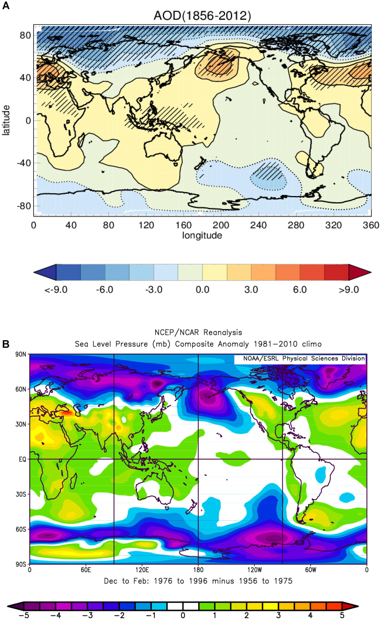
FIGURE 1. (A) The AOD (for volcano) signal (max–min, hPa) using a MLR technique on SLP (DJF) data for the period 1856–2012. Other indices used are ENSO, SSN and a longer term trend. Significant areas (95% significant) using a two-sided Student’s t-test are marked by hatching and negative contours are shown by dotted lines. (B) The result of SLP anomaly (DJF) plot from NCEP data for 1976–1996 with respect to reference level 1956–1975. Plot (B) is generated from the NOAA/ESRL Physical Sciences Division, Boulder Colorado web site at http://www.esrl.noaa.gov/psd/.

Influence of Natural Factors on Regional Temperature

Analysis of Observation

To address further on a mechanism, Figure 2 plotted mean difference of SST during 1976–1996 w.r.t. four other reference periods (of around 20 years each). Recent anomaly period 1999–2017 (Figure 2A) is also considered. Interestingly, in spite of a linear trend in SST, warming around central Pacific is noticed in all cases, even when reference period is recent years (Figure 2A). A consistent pattern is noticed in all four cases: a strong cooling around the north Atlantic (even more than 0.6K for most cases), warming in Aleutian Low (AL) and warming in Niño 3.4 region (of a range 0.4K and more). The cold SST signature around north Atlantic is consistent with positive NAO pattern. This signal also remains similar using the period 1976–1998, which adds two extra years (Supplementary Figure S1). The longer-term global warming signal (linear) is captured in most parts for all four plots with an exception of Niño regions connecting AL and North Atlantic region (it even shows cooling).

FIGURE 2

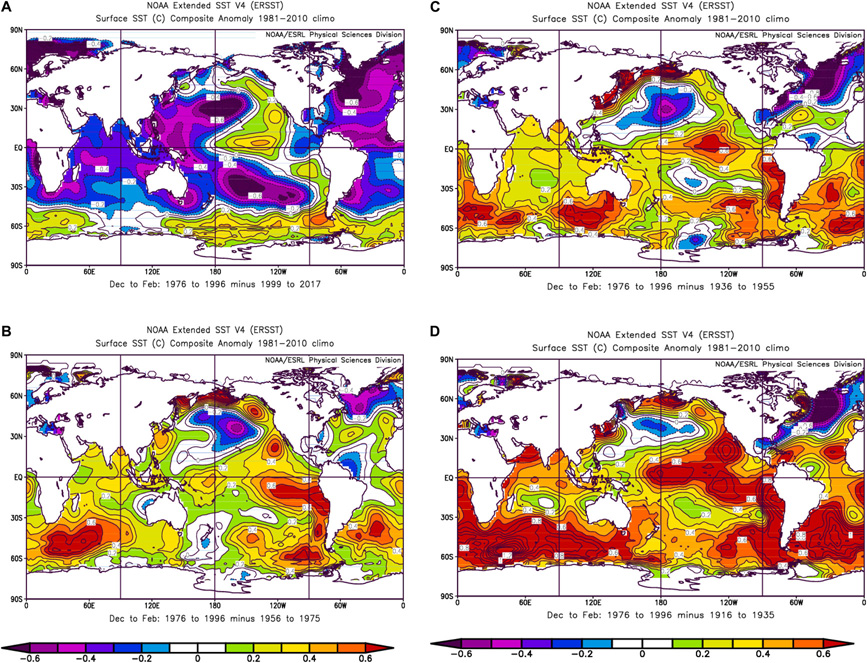
FIGURE 2. SST anomaly (DJF) from NOAA Extended SST V4 (ERSST), for 1976–1996 with respect to different reference levels: (A) 1999–2017, (B) 1956–1975, (C) 1936–1955, and (D) 1916–1935, respectively. Plots are generated from the NOAA/ESRL Physical Sciences Division, Boulder Colorado web site at http://www.esrl.noaa.gov/psd/.

Perturbations around North Atlantic was noted as a precursor of CP ENSO (Ham et al., 2013a,b) and the mechanism involves atmospheric Rossby wave. Positive NAO via triggering Rossby wave around mid-latitudes can influence north Pacific (AL is likely to be modulated) and subsequently has the potential to initiate CP ENSO through the atmospheric and oceanic bridge (for e.g., Equatorial Ocean Advection Theory (Kug et al., 2009) and Extra-tropical Forcing Theory (Yu et al., 2010; Kao and Yu, 2009; Yu and Kim, 2011). Ocean Advection Theory proposes that by the zonal ocean advection, anomalous SST along the equatorial region of Pacific is grown; while the other theory of ‘Extratropical Forcing’ indicates that the excitation is initially originated via a forcing from extra-tropics and later developed by the advection from the tropical Pacific. Our observation supports a chain of hypotheses: positive NAO – incite atmospheric Rossby wave to influence AL- via atmosphere/oceanic bridge trigger CP ENSO (Figures 2A–D). An oceanic/atmospheric pathway connecting AL and Central Pacific is very distinct (for SST) in all four plots. It is thus consistent with the findings of (Ham et al., 2013a,b) and also in favor of Extra-tropical Forcing Theory (Kao and Yu, 2009; Yu et al., 2010; Yu and Kim, 2011) and Equatorial Ocean Advection Theory (Kug et al., 2009) for CP ENSO formation. The Current analysis thus suggests that period 1976–1996 shows some special features, involving the NAO, AL and CP ENSO, which are different to that from a longer-term CO2 led linear trend and needs attention.

Further analysis was carried using surface ‘air temperature’ instead of SST with a new data set GISTEMP1200 (Figures 3A–D). Similar signals around north Atlantic, AL covering up to Niño 3.4 region is clearly distinguished. It strengthens the finding involving natural influences which are distinct to that from CO2 led linear trend. Interestingly, it also identifies a very strong warming around Eurasian snow cover, discrete from a longer-term linear trend. A similar signed warming signal (red) is noticed around the Eurasian sector, in all four plots of Figure 3 (even using anomaly period of recent years in Figure 3A).

FIGURE 3

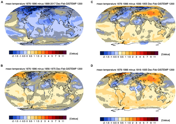
FIGURE 3. Same as Figure 2 (A–D) respectively, but for mean air temperature using observation from GISTEMP 1200. Plots generated using the IPCC’s Climate Change Atlas, climexp.knmi.nl/plot _atlas_form.py. Signal smaller than one standard deviation of natural variability is shown by hatching.

To check the robustness of identified signals on surface air temperature, two different datasets (HadCRUT4.2 and ERA-interim) are also tested (Supplementary Figure S2). It only compared anomaly period 1976–1996 with respect to the recent time (since 1999). It again verified that signals around north Atlantic, AL, CP ENSO and Eurasian snow cover are indeed robust for the period 1976–1996 and different from CO2 led linear anthropogenic influences.

Analysis of CMIP5 Models

To compare with observation, a model ensemble from AR5 CMIP5 subset models are used (Figure 4). Results (1976–1996) using only two different anomaly periods are presented (1999–2017) (Figure 4A) and 1956–1975 (Figure 4B). No specific features around north Atlantic, AL, CP ENSO and Eurasian snow cover are identified. In contrary to observation, Figure 4A is dominated by blue; whereas, Figure 4B by red. Such signal in the model ensemble is nothing but to represent a longer-term linear trend arisen out of CO2 led linear anthropogenic influences. An anomaly period of 1936–1955 is also considered which again suggests red indicating a similar linear trend (Supplementary Figure S3).

FIGURE 4

FIGURE 4. Mean temperature anomaly (Dec-Feb) for 1976–1996 with respect to reference level (A) 1999–2017 and (B) 1956–1975 considering AR5 CMIP5 subset models ensemble. Plots are generated using the IPCC’s Climate Change Atlas, climexp.knmi.nl/plot _atlas _form.py. Signal smaller than one standard deviation of natural variability is shown by hatching.

To test individual model performances, two arbitrary model (IPSL-CM5A-LR and NorESM1-M) results are presented for surface air temperature (Figure 5). Those two model results are presented as those suggest opposite signature around tropical Pacific. As seen, none of the individual two models captures the observed behavior for the period 1976–1996. Niño 3.4 temperature region in IPSL-CM5A-LR is dominated by blue for both the anomaly period (Figures 5A,B), while it is red for the model NorESM1-M (Figures 5C,D). Around a similar period, two models are also suggesting differently. For rest other CMIP5 models, all indicate varied spatial patterns and do not show any consistency among each other, let alone with observations and hence not shown. Some models, however, suggest similar signed signature around tropical Pacific, as observed, but fail to identify opposite signature around North Atlantic (as seen here for NorESM1-M). On the other hand, some models if match around the north Atlantic but disagree in Niño 3.4 region.

FIGURE 5

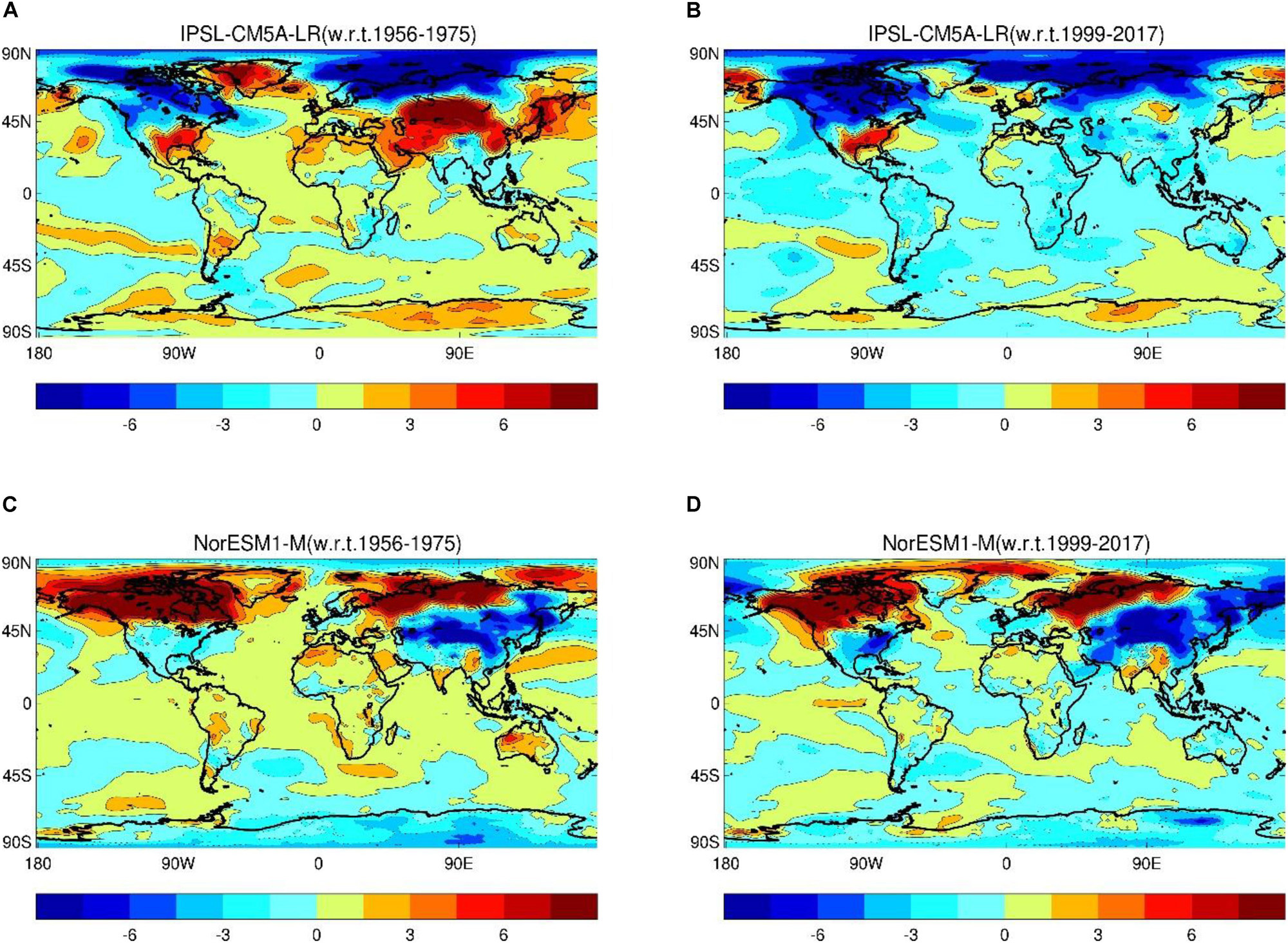
FIGURE 5. Mean surface temperature (DJF): 1976–1996 minus 1956–1975 (Left); 1976–1996 minus 1999–2017 (Right) for two arbitrarily chosen CMIP5 models, IPSL-CM5A-LR (top) and NorESM1-M (bottom).

The similar varied pattern of ISM rainfall is also noted by Roy (2017) that used 23 most commonly used CMIP5 models. That study compared observed decreasing rainfall trend around central north east (CNE) India with CMIP5 model results. To present diverse behavior among models, results were presented starting with positive patterns and ending with the negative pattern, with models without much indications in between. Similar inconsistency in CMIP5 model results with observation was also identified by Turner and Annamalai (2012), where they discussed about the cause of discrepancy and indicated improper modulation of decadal signature in models as one potential factor. Other probable candidates identified for similar disagreement are circulation-based changes (Roxy et al., 2015), aerosol-based changes [Bollasina et al. (2011) and sea-surface temperatures in the Indo-Pacific (Roxy et al., 2015)].

Influence on Humidity

Analyses on specific humidity for the period 1976–1996 is carried w.r.t. an anomaly period (1999–2017) (Figure 6). Note here the reverse color bar. Model ensemble suggests less water vapor throughout (Figure 6A) which is consistent with cooling as noticed in Figure 4A. On the contrary, observation using ERA-Interim shows diverse regional impact (Figure 6B), agreeing with observed surface air temperature anomaly pattern. As expected, more water vapor is accumulated around the central and eastern Pacific. In contrast to model, results from Reanalysis is dominated by blue (and hence more water vapor). If the anomaly period considered is (1956–1975) (Supplementary Figure S4), the model ensemble also conforms to its temperature signature (Figure 4B). Noting the water vapor as the major GHG (Kiehl and Trenberth, 1997), its contribution during later two decades of last century and Hiatus period is clearly established. Also, the GHG effect from water vapor is seen not linear but dominant during period 1976–1996. It explains why temperature trend in model ensemble could deviate to that from observational records during warming Hiatus period. Moreover, it points that it could be the preferential alignment of ENSO positive phase during the period 1976–1996, and associated water vapor feedback that could be a prime factor for an abrupt rise in global temperature.

FIGURE 6

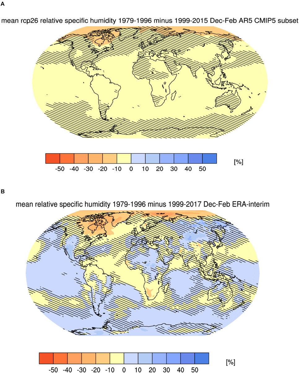
FIGURE 6. Mean specific humidity anomaly (1979–1996 minus 1999–2017) for Dec-Feb from (A) AR5 CMIP5 subset models and (B) ERA-interim data. It started from 1979 instead of 1976 because ERA-interim data are only available since then. Areas with signal smaller than one standard deviation of natural variability is shown by hatching. Plots generated using the IPCC’s Climate Change Atlas; climexp.knmi.nl/plot _atlas_form.py. Note here the reverse color bar.

Results from same two individual CMIP5 models (IPSL-CM5A-LR and NorESM1-M) are also presented (Supplementary Figures S5A,B). An anomaly of specific humidity for period 1976–1996 is calculated w.r.t. 1956–1975. Model IPSL-CM5A-LR suggests less water vapor around Niño3.4 region; whereas, NorESM1-M shows an abundance. However, individual models are in accordance with the humidity-temperature known connection in Niño3.4 region, i.e., rise (fall) in temperature (Figures 5A,C, respectively) will normally be linked with a rise (fall) in humidity (Supplementary Figures S5A,B, respectively). Similar to SST, representation of humidity also fails to indicate consistency among various CMIP5 models, and hence not shown.

Time Series Analyses

In terms of the Sun and volcano, how time series of the observed ENSO and global temperature follow are presented Figure 7. The ENSO, measured by Niño 3.4 is seen in phase with observed global temperature series, with their peaks and troughs matching with each other. The Niño 3.4 suggests more variability during the period 1976–1996 (shown in between dotted lines in Figure 7) as also noted by Qiong et al. (2008). That period is dominated by warm peaks of ENSO; whereas cold peaks are more prominent since 1999.

FIGURE 7

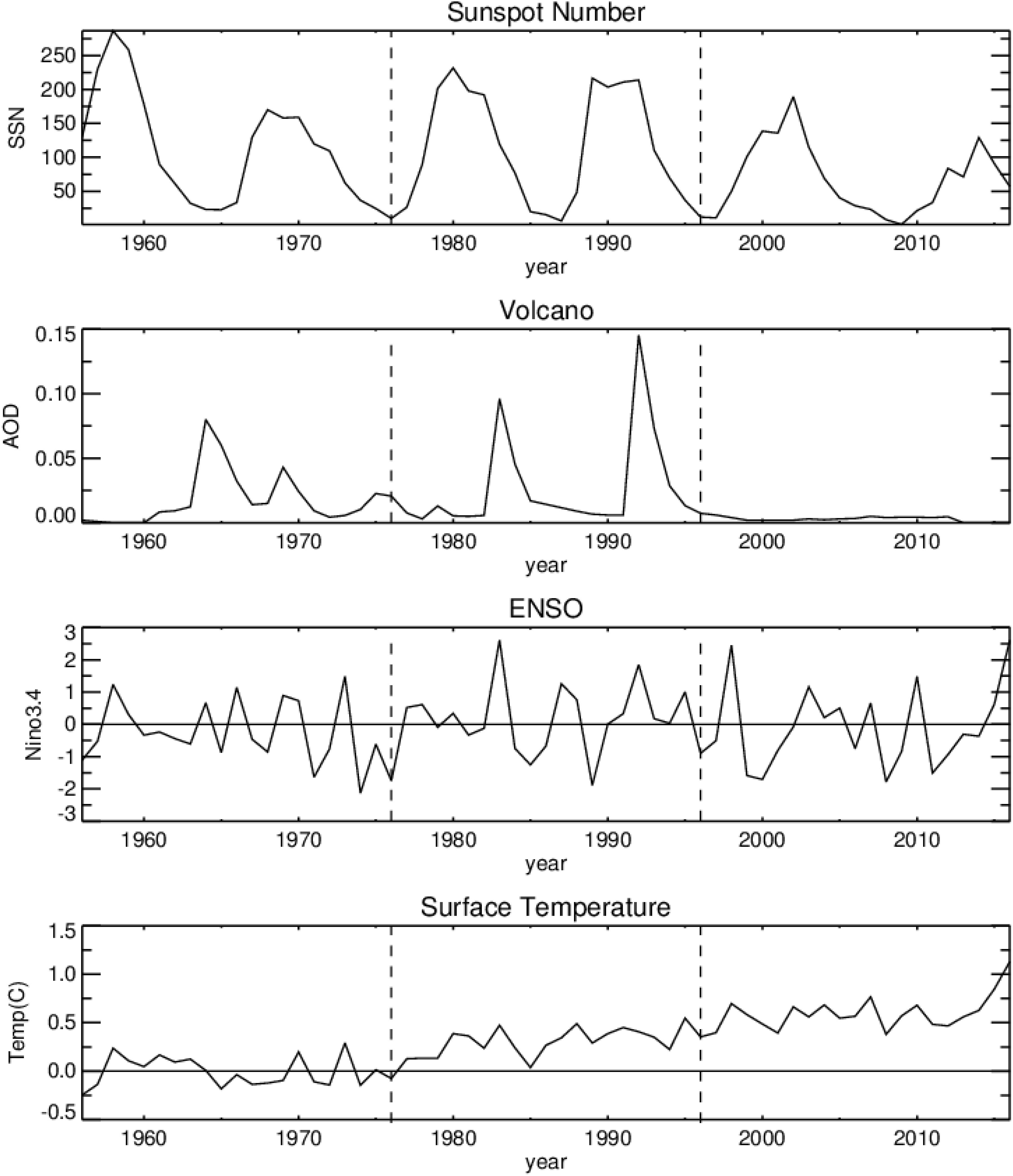
FIGURE 7. Observed time series of various natural factors (solar cycle variability, volcano and ENSO) and global surface temperature. Solar cycle variability is represented by SSN, volcano by AOD and ENSO by Niño3.4 indices. The period 1976–1996, the time of abrupt global warming is marked by dotted lines. The period exceeding the right dotted lines represent the warming slowdown period. The warming in 2016 is distinct and it is seen linked with the strong El Niño of 2016.

Figure 8 presented few time-series from reanalyses and CMIP5 model outputs. It showed global specific humidity observed from reanalyses product ERA-Interim (top panel) and also presented model ensemble behavior for global specific humidity, global temperature and Niño 3.4, respectively. The model ensemble (and also almost all individual models) shows a clear rising trend for all those three parameters in recent period to that from 1976 to 1996. Thus models suggest consistency in terms of global features and follow the known connection between these three parameters. It indicates that rise in Niño 3.4 temperature trend will cause more water vapor content and more rise in global temperature. Interestingly, observation suggests differently. There is no rising trend noticed for either observed ENSO (Figure 7) or global specific humidity (Figure 8, top panel). Global temperature, however, suggests a rise in observation as well as models. The post-volcanic cooling as noted in the model ensemble for temperature, (by two sharp troughs, Figure 8) is however, not identified in observation (Figure 7, bottom panel). In observation, only a sharp trough is noticed at 1985, between two dotted lines, which could be probably due to the strong La Niña of 1985.

FIGURE 8

FIGURE 8. Time series plots (Dec-Feb) of various meteorological parameters from reanalyses product (top plot) and CMIP5 models. Anomaly period considered is 1980–2010. The top plot is for specific humidity from ERA Interim, and the rest three are from AR5 CMIP5 subset models for global specific humidity, global temperature and near-surface temperature in Niño 3.4 region, respectively. For models, one line per model is shown by thin lines, while multi-model mean is marked by a thick line. On the right, the spread associated with various RCP scenarios over 1986–2016 are shown. Horizontal line denotes the median (50%) of the whole dataset, the box extends from 25 to 75% and the whiskers from 5 to 95%. White mark within the plots of model results indicates the start of RCP scenarios. Plots are generated using the IPCC’s Climate Change Atlas; climexp.knmi.nl/plot _atlas_form.py.

To analyze further, I present Table 1 where results of only seven models are presented, starting with two chosen models, IPSL-CM5A-LR and NorESM1-M. The rest almost all models suggest the same and hence not shown. It indicates a decrease in observed Niño 3.4 temperature and a subsequent decrease in global specific humidity in recent period to that from 1976 to 1996. The deviation in the recent period, however, is completely opposite (positive) for all models (last column Table 1). As the ERA-Interim data for relative humidity is present upto 2011, the calculation for Niño 3.4 using observation was carried upto 2011, as well as upto 2016. Even including the strong El Niño of 2016, the negative anomaly during a recent period is still clear. On the other hand, if the analyses for models are restricted upto 2011 instead of 2016, the same consistent pattern is noticed. To highlight further, the difference between results of the model to that from Observation/Reanalysis, I present Figure 9. It considers the value from the last column of Table 1. Models those indicate higher Niño 3.4, also suggest higher specific humidity and vice versa in Figure 9. It clearly identifies the difference between observation and model results, which are completely opposite, and suggests models in general, are overestimating global water vapor contents in recent periods. Such contributions are most likely to add additional warming due to greenhouse gas, and a subsequent rise in global temperature in models.

TABLE 1

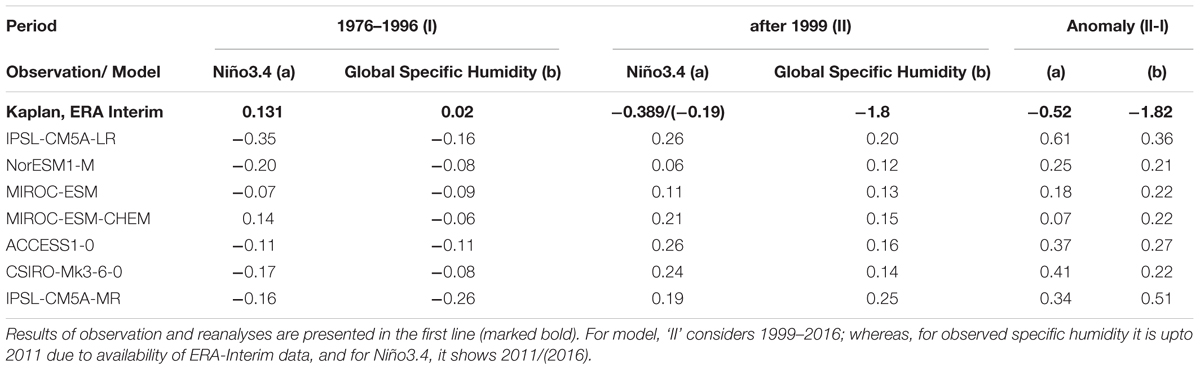
TABLE 1. Variation of Niño 3.4 and Global Specific Humidity (gm/kg) anomaly in abrupt warming period (1976–1996) and warming trend slowdown period.

FIGURE 9

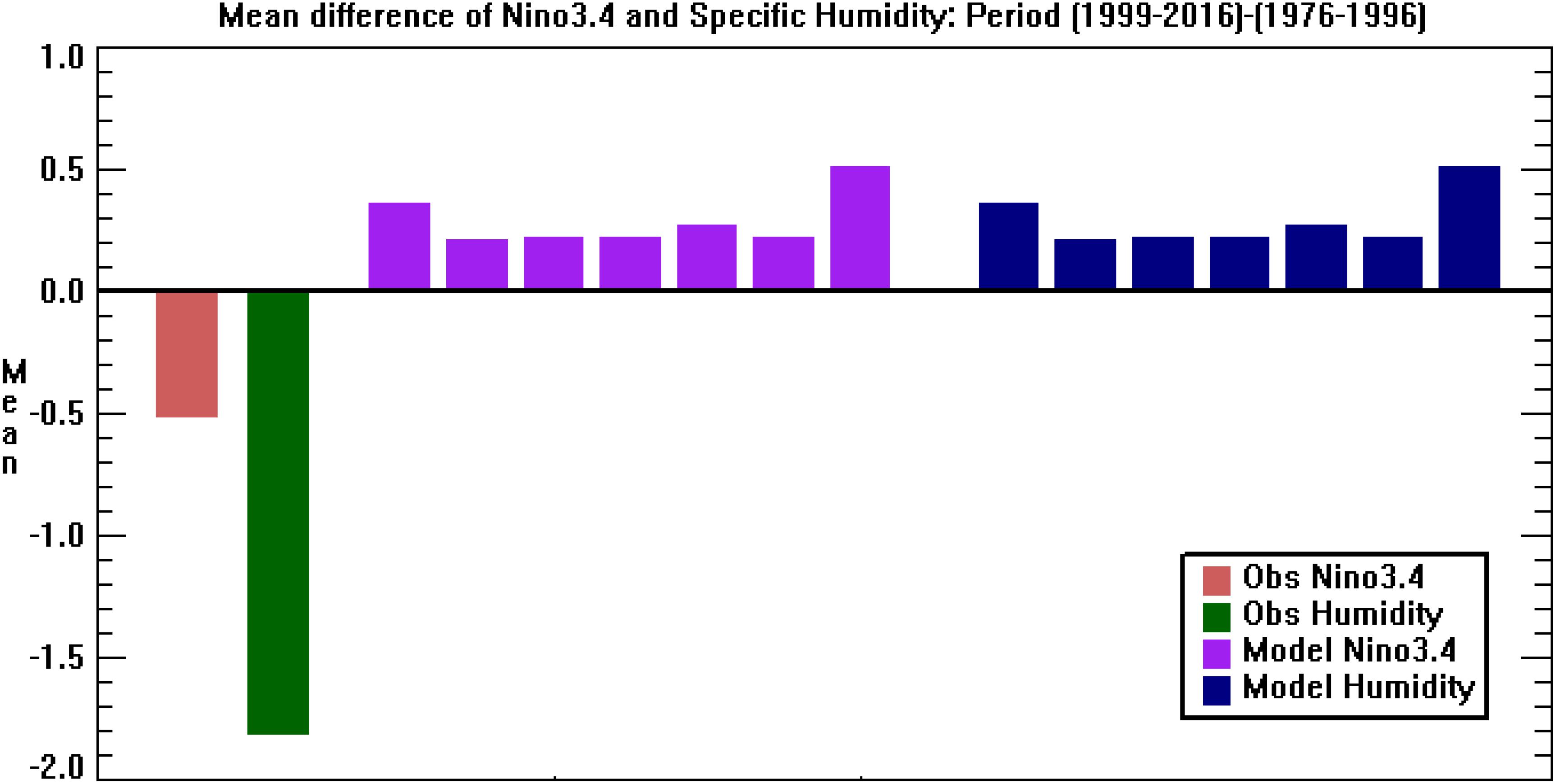
FIGURE 9. Mean difference of Niño3.4 and specific humidity from period after 1999 to that from 1976 to 1996. First two bar plots are for Niño3.4 and specific humidity, respectively, from observed or reanalyses products. Results for seven different models are presented, purple for Niño3.4 and blue for specific humidity. Models shown are IPSL-CM5A-LR, NorESM1-M, MIROC-ESM, MIROC-ESM-CHEM, ACCESS1-0, CSIRO-Mk3-6-0 and IPSL-CM5A-MR, respectively. For rest other models, almost all suggest similarly and hence not shown.

Time series plots of various model Niño 3.4 temperatures are also presented along with the observed Niño 3.4 series (Supplementary Figure S6). It highlights the diverse behavior of ENSO among models, where the model Niño 3.4 peaks and troughs are seen very unlike to match with each other, let alone with the observation. The observed ENSO, (first plot) suggests more bias toward warm ENSO phase and shows a stronger variability during the period 1976–1996 (shown in between two vertical dotted lines) to that from any other intervals. Observed Niño 3.4 also do not suggests any clear rising trend in a recent period, the period after the red dotted line. In contrary to observation, almost all models indicate a rise in Niño 3.4 in recent periods to that from 1976 to 1996 and do not follow observed ENSO behavior, as discussed.

Exploring on the Sun and ENSO Behavior

To examine further, I explore the connection between individual drivers - here the focus is on the Sun and ENSO behavior. The observed results as noted in Roy and Haigh (2012), and Roy (2014) are reproduced updating both the SSN (also used the new SSN data of version 2) and Niño 3.4 data. This is a plot of ENSO (DJF) against SSN and results of observation and those two models (IPS-CM5A-LR and NorESM1-M) are presented (Figure 10). Peak or max year from all solar cycles are marked by red squares. When SSN is high, say, above ∼120 (1.9 standard deviations of SSN is 122), a bias toward a cold event side of the ENSO is noticed in observation. Exceeding that SSN threshold, all 12 solar max or peak years lie on the cold event side. Such feature is not present in models (Figure 10A). During all solar max years, Niño 3.4 values in models also differ to that from observation, as seen by the individual positioning of red squares. In terms of the sun and ENSO behavior, it also confirmed another interesting feature from the study of Roy and Haigh (2012), and Roy (2014). It showed that if we segregate out the period 1957–1997, not only solar max years, but all years above high SSN values (say above ∼120) lie on the cold event side of ENSO (Figure 10B). During period ‘1856–1957 and 1998–2016,’ not a single point lies in the top right quadrant, though points are near equally distributed in all four quadrants in the intervening period of 1957–1997. Chosen models do not comply with such observation. Other models also suggest similarly and hence not shown. As the purpose is to verify those previous results, hence similar intervening time periods as used there are presented. Also, note that the value of SSN threshold (∼120) has changed here due to the use of new version (2) of SSN data.

FIGURE 10

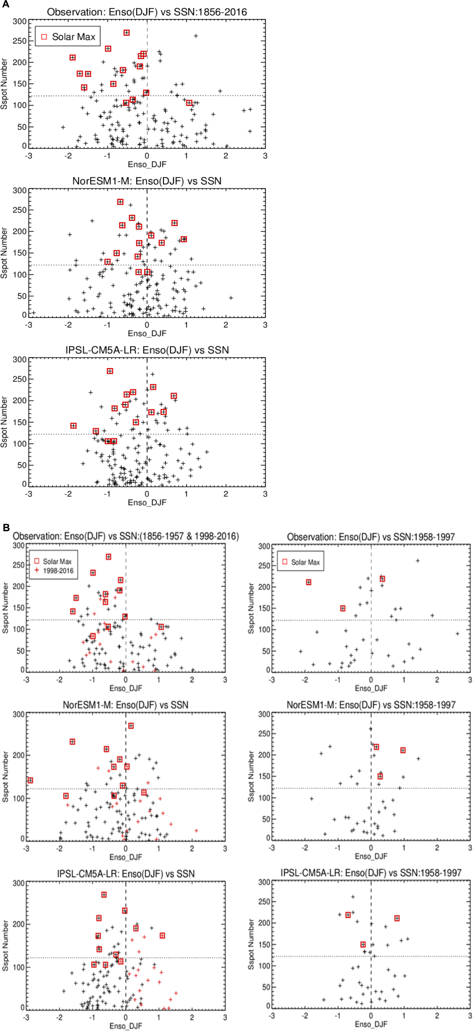
FIGURE 10. Average ENSO (Dec-Jan-Feb) against annual average Sunspot number (SSN). Observed Niño 3.4 index is used in the top row of each plot, while bottom two rows use Niño 3.4 temperature for CMIP5 models NorESM1-M and IPSL-CM5A-LR, respectively. In (A) it considers the whole period of observed record (1856–2016) and in (B) it separates out an intervening period (1958–1997) from the whole set of observation. The right panel in (B) is for period ‘1958–1997’ and the left for ‘1856–1957 and 1998–2016.’

Some Lead-Lag Analyses Involving ISM

Several studies (Liu and Yanai, 2001; Xavier et al., 2007) showed that winter NAO has a strong modulating effect on ISM. The period the relationship between the ISM and ENSO has weakened, the connection between the temperature of West Eurasia and ISM turned stronger (Chang et al., 2001). According to them, as the ENSO ISM teleconnection became weaker, the possibility for the NAO to influence the ISM through the above mechanism has enhanced.

To study the teleconnection between various temperatures related fields and ISM rainfall, some lead-lag analyses are performed (Figure 11). For temperature fields, I consider three different locations: the region of Niño 3.4, a location from the Eurasian sector (40°N to 60°N, 70°E to 100°E) and also a region around the North Atlantic (40°N to 60°N, 50°W to 30W°). From the Eurasian sector and the north Atlantic, I chose an arbitrary location each, which suggested a stronger observed temperature anomaly during 1976–1996. For ISM, the main interest is around regions of the CNE India and its surroundings. This is the location of strengthened ITCZ (Intertropical Convergence Zone) during JJAS, receives intense heating and serves as the meeting point of both the Walker circulation and regional Hadley cell (Gill, 1980; Goswami, 1994). The area covering CNE region received enough interest in latest studies (Bollasina et al., 2011; Roy et al., 2017; Roy, 2017). For the Niño 3.4, in both DJF and JJAS, a significant anti-correlation is noticed in that location, which is stronger when Niño 3.4 for JJAS is considered (first and second row). The connection is seen also strengthened in the recent period. However, when the Eurasian sector is considered, its connection with ISM in CNE region is completely reversed in recent period to that from 1979–1996. Using a temperature of north Atlantic, similar reversal of correlation pattern of ISM is noticed around CNE India, though it is not significant. Due to a closer proximity of Eurasian sector to India, its effect seems stronger than the effect from the north Atlantic. It is very likely that a strong temperature anomaly around the northern part of regional Hadley circulation can modulate the other end of the circulation, which passes through the ITCZ and also covers the CNE region of India.

FIGURE 11

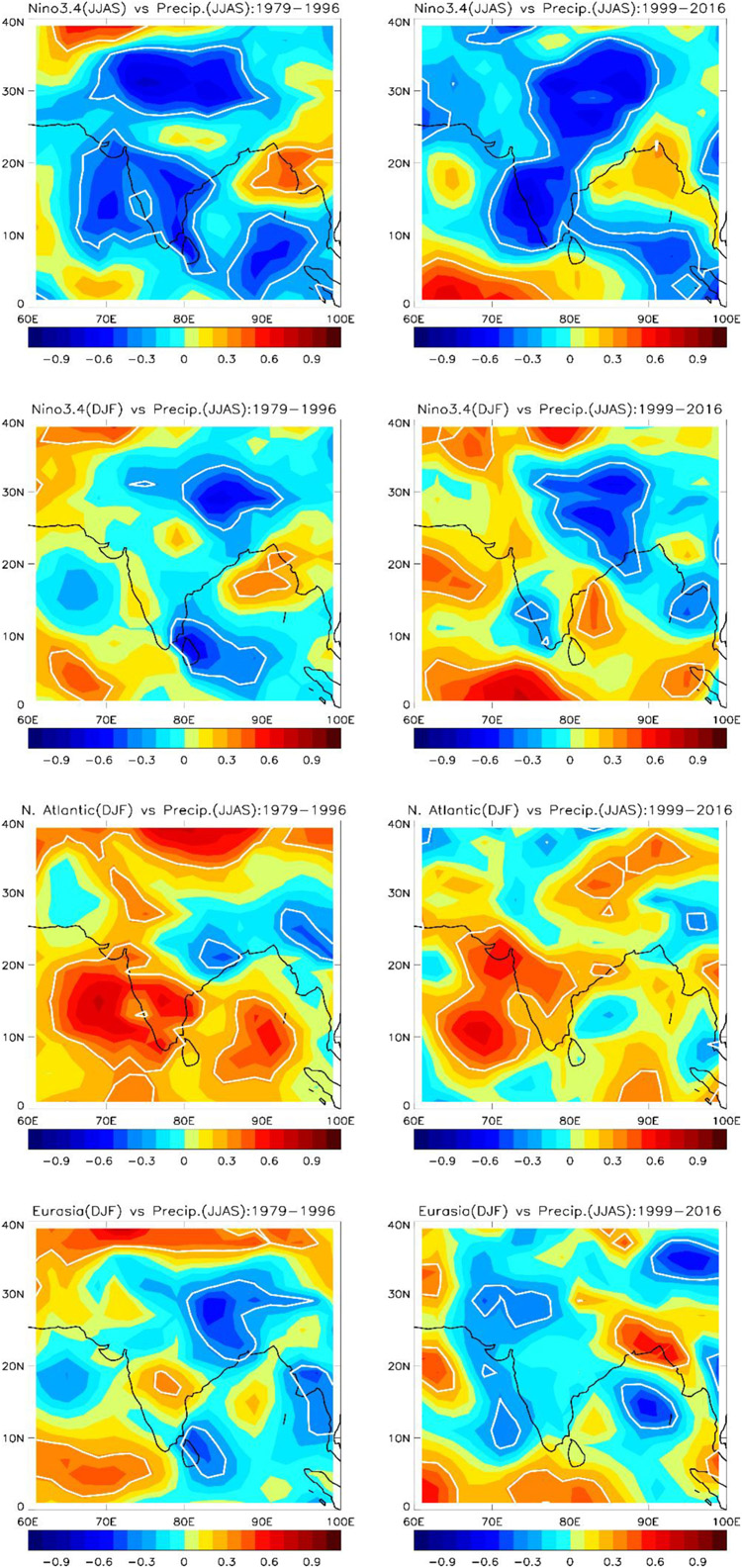
FIGURE 11. Correlation between various temperatures related fields and Indian Summer Monsoon (ISM) rainfall (in JJAS) and some lead-lag analyses. The top two panels use Niño 3.4 temperature and the bottom two for the temperature of North Atlantic and Eurasian sector, respectively. The top panel shows correlation using Niño 3.4 temperature of JJAS, while the bottom three panels consider temperature fields of DJF. Left panel for 1979–1996 and the right for 1999–2016. Significant regions at 95% level, using a student’s t-test are marked by white lines.

Proposing a Mechanism

Figure 12 considers a latitudinal slice 50–70°N and shows that during period (1976–1996) (w.r.t. 1999–2017) for DJF, the observed cooling over the north Atlantic is not only restricted to surface level. The cooling even extends high in the upper troposphere. Consistent to that, geopotential height suggests a strong negative anomaly in the vertical column, exceeding 55 m around upper troposphere. Such anomaly pattern has the potential to modulate mid-latitude planetary scale Rossby waves around the north Atlantic and subsequently can impact AL.

FIGURE 12

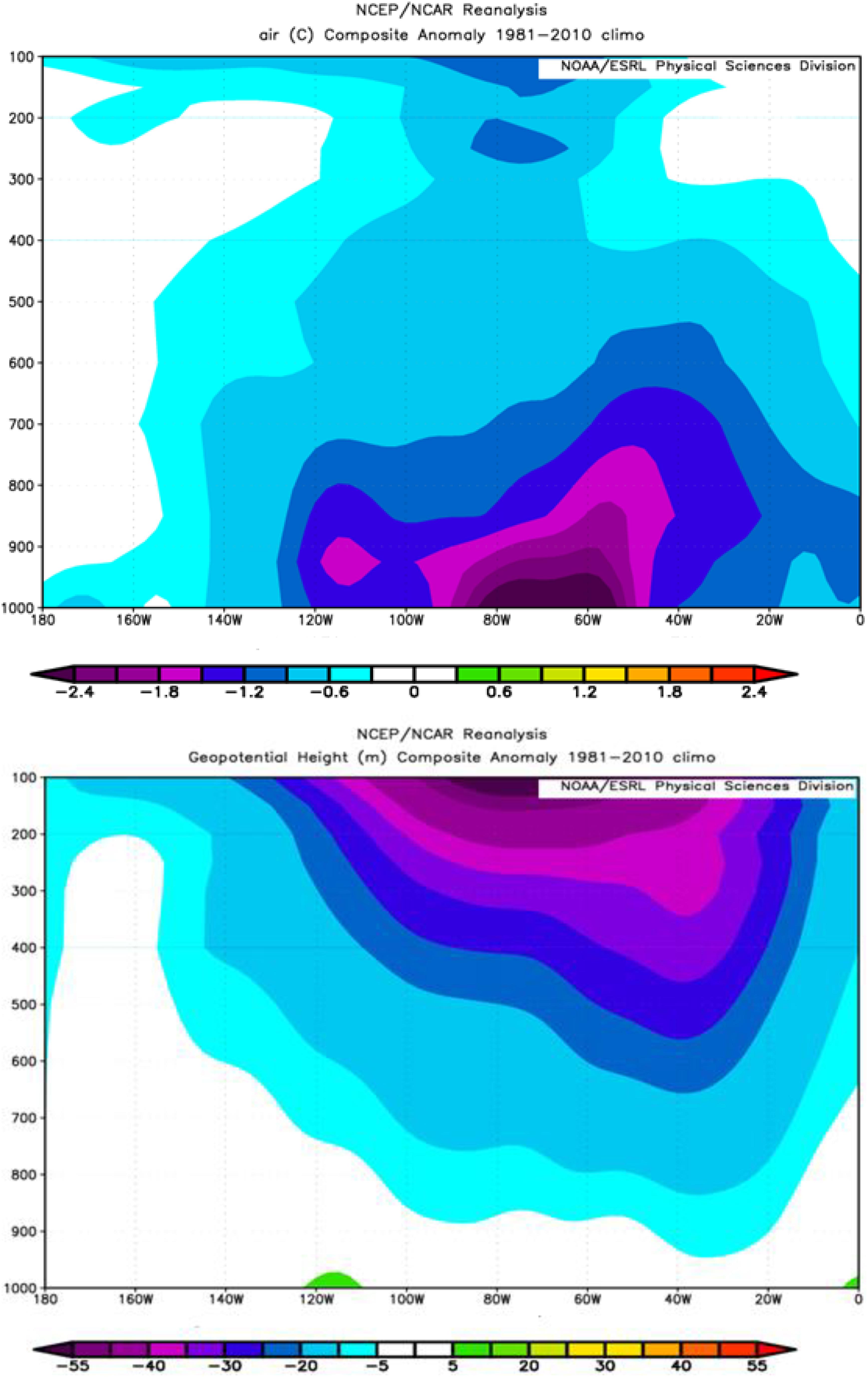
FIGURE 12. Longitude vs. Height anomaly plot for Dec-Feb, (1979–1996 minus 1999–2017) averaging over 50°N to 70°N. Parameter used are air temperature, and geopotential height, respectively, as shown in subtitles. Plots are generated by the NOAA/ESRL Physical Sciences Division, Boulder Colorado from their Web site at: http://www.esrl.noaa.gov/psd/.

A schematic is proposed (Figure 13) to outline hypothesized mechanisms initiated by explosive volcanism during later two decades of last century (1976–1996). Amplifying the effect on positive NAO phase (Figures 1A,B, 12), it influences extra-tropical Atmospheric Rossby waves and via AL and oceanic, atmospheric bridge it has a modulating effect on CP ENSO (Ham et al., 2013a,b). Those pathways are also noted using results from various observational and reanalyses products (Figures 2, 3 and Supplementary Figures S1, S2). CP ENSO became more persistent and frequent since the 1970s (Ashok and Yamagata, 2009; Yeh et al., 2009), though reverted back after late 1990s. Solar decadal variability was also identified around those locations [north Atlantic for NAO: Roy (2016); AL: (Roy and Haigh, 2010, 2012); CP ENSO: Sullivan et al. (2016)]. However, this work points toward the role of explosive volcanos (Figure 1A) during the active solar phase and studies the combined influence of natural forcing (Figures 1A,B). Interestingly, during those decades there was an enhancement of CP El Niño variability even when data from last eight centuries were considered (Liu et al., 2017).

FIGURE 13

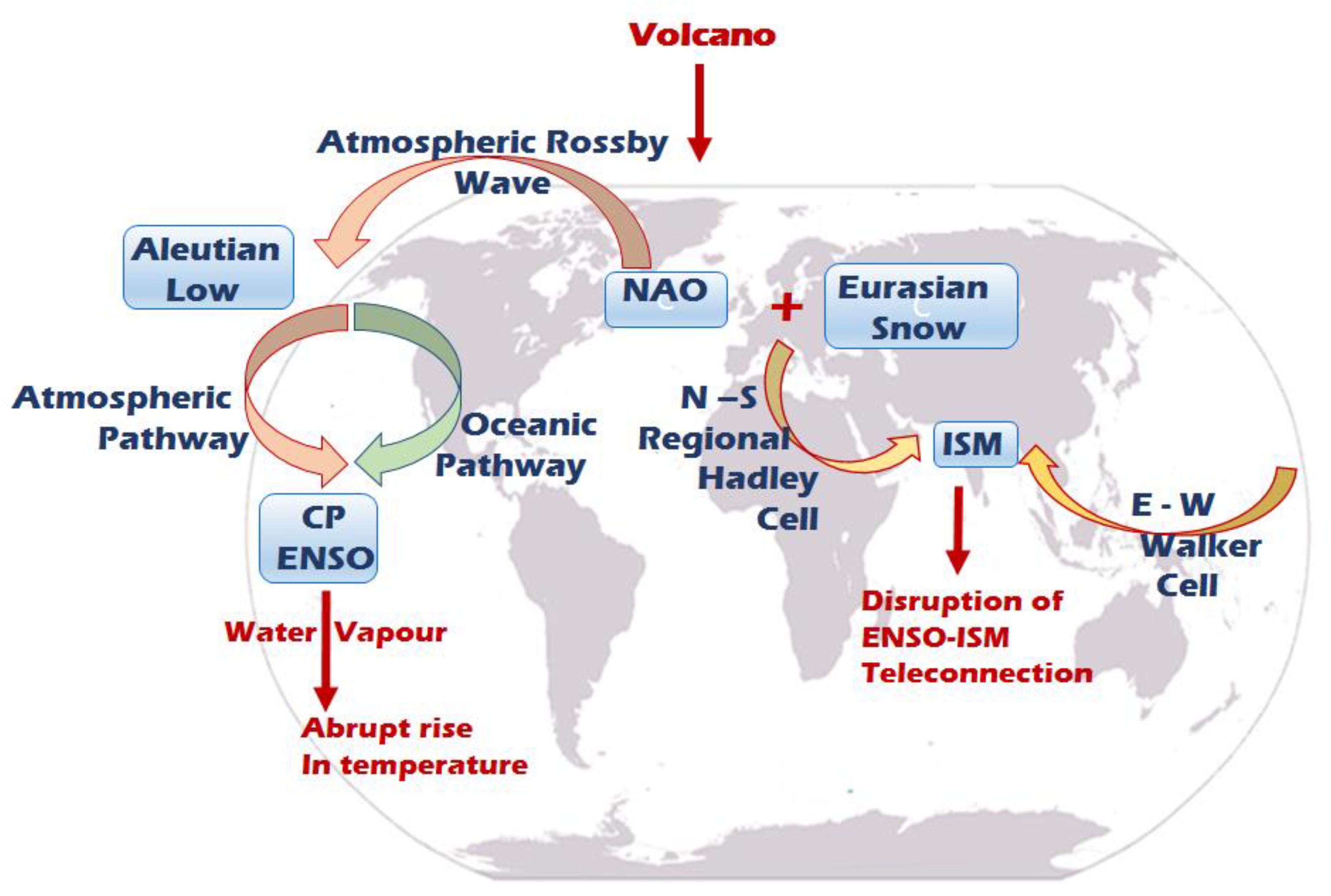
FIGURE 13. A schematic of mechanisms initiated by explosive volcanism during 1976–1996. It modulates various modes (NAO, ISM and CP ENSO) and influences various places (AL and Eurasian snow cover), shown by blue box. AL is impacted from North Atlantic via Atmospheric Rossby waves. That signal is transported to trigger CP ENSO via Atmospheric (pink arrow) and Oceanic pathways (green arrow). CP ENSO increases atmospheric water vapor causing abrupt rise in global temperature (shown by red). Combination of NAO and Eurasian Snow strongly modulate regional N-S Hadley circulation (yellow arrow) to impact ISM. Usual ENSO-ISM teleconnection via E-W Walker circulation (yellow arrow) is thus overtaken suggesting a disruption in ENSO-ISM teleconnection (shown by red).

It also supports Adams et al. (2003) and Ohba et al. (2013), those indicate volcanic forcing drives the coupled ocean-atmosphere system more subtly toward a preferential direction, where multi-year El Niño-like situations (measured by Niño 3.4 temperature) are favored. The number of El Niño during that period outnumbered to that of La Niña with a significant rise of its variability and duration (Trenberth and Hoar, 1996; Qiong et al., 2008). El Niño phase is associated with warm global temperature (Sobel et al., 2002), it could be due to more water vapor content in the atmosphere. As water vapor is the most powerful GHG (Kiehl and Trenberth, 1997), our analyses of Figures 7–9 and Table 1 explains the puzzle of global warming hiatus and also clarifies an abrupt rise in global temperature during 1976–1996.

Positive NAO phase and Eurasian snow cover both show dominance during that period (1976–1996) as shown in Figures 1B, 2, 3, and Supplementary Figures S1, S2. The possibility for the NAO and Eurasian snow cover to influence the ISM by modulating the regional N-S Hadley circulation may have overpowered the known teleconnection generated due to E-W Walker circulation (Kumar et al., 1999). It is noted that the period when ISM-ENSO known anti-correlation became weakened, the connection between the temperature of West Eurasia, NAO and ISM turned stronger (Chang et al., 2001). It explains why ISM-ENSO connection strengthened again in recent days. Analyses using observed ISM data of Figure 11 are in agreement with such pattern. Though the proposed pathways are in agreement with popular research and supported by existing theories but to test those in more details are beyond the scope of current analyses and it will be addressed in a subsequent study.

Model results (Figures 4, 5, 6A, 9 and Supplementary Figures S3–S5), however, disagree with observations and hence do not support hypothesized mechanism. As the phasing of models for Niño 3.4 temperature and other parameters do not match with observed series (Supplementary Figure S6), the models are likely to indicate a diverse regional pattern and to miss the proposed teleconnection pattern as discussed in Figure 13. Driscoll et al. (2012) also discussed that following eruption, models fail to capture the Northern Hemispheric dynamical response. One possible explanation of such disagreement could be that CMIP model simulations do not follow the same phasing of natural climate variability (that also include decadal variability) with observation (Turner and Annamalai, 2012; Santer et al., 2017). Current analyses also addressed those issues. Roy (2017) also discussed how the ENSO and ISM phase in CMIP5 models vary from observation. In spite of the fact that CMIP5 models differ with observation in terms of phasing of various modes of climate variability, we show here those also fail to recognize shifting of important major climate features at later decades. Hence the question arises about the reliability of CMIP5 model results of global temperature series. The purpose of this study is also to pinpoint those areas for improving model performances.

Discussion and Summary

The puzzle of global warming hiatus is discussed in many recent studies, though the underlying cause is still unexplained. Many climate features, in atmosphere and ocean including global temperature trend, suffered deviations during later two decades of the last century, so as some known teleconnection patterns. This study addresses those areas segregating the role of natural factors (the sun and volcano) to that from CO2 led linear anthropogenic influences. To analyse the combined influence of the sun and volcano (including the phasing), it separated out a period 1976–1996 that captured two full solar cycles, (number 21 and 22), where two explosive volcanos erupted (1991 and 1982) during active periods of strong solar cycles.

The possible mechanism could be initiated via a preferential alignment of NAO phase, generated by explosive volcanos. During that particular period, it identified certain deviations on various climate features, those include temperature around Niño 3.4 region (warming), North Atlantic region (cooling), AL (warming) and Eurasian snow cover (warming). The robustness of detected signal is established by analyzing different observational and reanalyses datasets. Consistent with temperature, a dominance of atmospheric water vapor content is also noticed. Interestingly, CMIP5 model ensemble (and also arbitrarily chosen individual models) fails to comply with such findings. It is also true for other models. This study indicates that water vapor being the most important GHG has major contributions for an observed abrupt rise in global temperature during that period. Overall the analysis suggests a change in CP ENSO and associated water vapor feedback plays a very important role in regulating global temperature behavior since 1976 that also includes ‘Hiatus’ period. It identified the signal of natural origin is different to that from CO2 led anthropogenic linear influence. Interestingly, models suggest a failure to detect such signals, which provides explanations for the long-standing puzzle of global warming hiatus.

It also discussed mechanisms how an anomaly in the north Atlantic can modulate CP ENSO features. Inciting extratropical atmospheric Rossby wave, NAO has the potential to influence the AL. It has a modulating effect on CP ENSO via the pathway of the atmospheric and oceanic bridge.

Disruption of ISM-ENSO teleconnection during the later decades of last century can also be explained from that angle. As positive NAO phase and Eurasian snow cover show dominance during that period, their possibility to influence the ISM by modulating the regional N-S Hadley circulation has overshadowed the known teleconnection generated due to E-W Walker circulation from ENSO. It is consistent with the finding that during that period when ISM-ENSO known anti-correlation became weakened, the connection between the temperature of West Eurasia, NAO and ISM turned stronger. It explains why ISM-ENSO teleconnection reverted back again in the recent period.

Author Contributions

IR has done the whole work.

Conflict of Interest Statement

The author declares that the research was conducted in the absence of any commercial or financial relationships that could be construed as a potential conflict of interest.

Supplementary Material

The Supplementary Material for this article can be found online at: https://www.frontiersin.org/articles/10.3389/feart.2018.00136/full#supplementary-material

Footnotes

1. ^http://cmip-pcmdi.Llnl.gov/cmip5/experiment_design.html
2. ^https://www.esrl.noaa.gov/psd/data/gridded/data.gistemp.html
3. ^http://www.esrl.noaa.gov/psd/

References

Adams, J. B., Mann, M. E., and Ammann, C. M. (2003). Proxy evidence for an El Niño-like response to volcanic forcing. Nature 426, 274–278. doi: 10.1038/nature02101

PubMed Abstract | CrossRef Full Text | Google Scholar

Allan, R., and Ansell, T. (2006). A new globally complete monthly historical gridded mean sea level pressure dataset (HadSLP2): 1850-2004. J. Climate 19, 5816–5842. doi: 10.1175/JCLI3937.1

CrossRef Full Text | Google Scholar

Ashok, K., Behera, S. K., Rao, S. A., Weng, H., and Yamagata, T. (2007). El Niño Modoki and its possible teleconnections. J. Geophys. Res. 112:C11007. doi: 10.1029/2006JC003798

PubMed Abstract | CrossRef Full Text | Google Scholar

Ashok, K., Guan, Z., and Yamagata, T. (2001). Impact of indian ocean dipole on the relationship between the indian monsoon rainfall and ENSO. Geophys. Res. Lett. 28, 4499–4502. doi: 10.1038/s41598-017-05225-z

PubMed Abstract | CrossRef Full Text | Google Scholar

Ashok, K., and Yamagata, T. (2009). Climate change the El Niño with a difference. Nature 461, 481–484. doi: 10.1038/461481a

PubMed Abstract | CrossRef Full Text | Google Scholar

Bollasina, M. A., Ming, Y., and Ramaswamy, V. (2011). Anthropogenic aerosols and the weakening of the South Asian summer monsoon. Science 334, 502–505. doi: 10.1126/science.1204994

PubMed Abstract | CrossRef Full Text | Google Scholar

Bond, N. A., Overland, J. E., Spillane, M., and Stabeno, P. (2003). Recent shifts in the state of the North Pacific. Geophys. Res. Lett. 30:2183. doi: 10.1029/2003GL018597

CrossRef Full Text | Google Scholar

Chang, C. P., Harr, P., and Ju, J. (2001). Possible roles of Atlantic circulations on the weakening Indian monsoon rainfall–ENSO relationship. J. Clim. 14, doi: 10.1175/1520-0442(2001)014<2376:PROACO>2.0.CO;2

CrossRef Full Text | Google Scholar

Compo, G. P., Whitaker, J. S., Sardeshmukh, P. D., Matsui, N., Allan, R. J., Yin, X., et al. (2011). The twentieth century reanalysis project. Q. J. R. Meteorol. Soc. 137, 1–28. doi: 10.1002/qj.776

CrossRef Full Text | Google Scholar

Driscoll, S., Bozzo, A., Gray, L. J., Robock, A., and Stenchikov, G. (2012). Coupled model inter-comparison project 5 (CMIP5) simulations of climate following volcanic eruptions. J. Geophys. Res. 117:17105. doi: 10.1029/2012JD017607

CrossRef Full Text | Google Scholar

Emile-Geay, J., Seager, R., Cane, M. A., Cook, E. R., and Haug, G. H. (2008). Volcanoes and ENSO over the past millennium. J. Clim. 21, 3134–3148. doi: 10.1175/2007JCLI1884.1

CrossRef Full Text | Google Scholar

Gill, A. E. (1980). Some simple solutions of heat induced tropical circulations. Q. J. R. Meteorol. Soc. 106, 447–462. doi: 10.1002/qj.49710644905

CrossRef Full Text | Google Scholar

Goswami, B. N. (1994). Dynamical predictability of seasonal monsoon rainfall: Problems and prospects. Proc. Natl. Sci. Acad. U.S.A. 60, 101–120.

Google Scholar

Gray, L. J., Scaife, A. A., Mitchell, D. M., Osprey, S., Ineson, S., Hardiman, S., et al. (2013). A lagged response to the 11 year solar cycle in observed winter Atlantic/European weather patterns. J. Geophys. Res. Atmos. 118, 405–413. doi: 10.1002/2013JD020062

CrossRef Full Text | Google Scholar

Ham, Y.-Y., Kug, J.-S., Park, J. Y., and Jin, F.-F. (2013a). Sea surface temperature in the north tropical Atlantic as a trigger for Ela/Southern Oscillation events. Nat. Geosci. 6, 112–116. doi: 10.1038/ngeo1686

CrossRef Full Text | Google Scholar

Ham, Y.-Y., Kug, J.-S., Park, J. Y., and Jin, F.-F. (2013b). Two distinct roles of Atlantic SSTs in ENSO variability: North tropical Atlantic SST and Atlantic Niño. Geophys. Res. Lett. 40, 4012–4017. doi: 10.1002/grl.50729

CrossRef Full Text | Google Scholar

Hansen, J., Ruedy, R., Sato, M., and Lo, K. (2010). Global surface temperature change. Rev. Geophys. 48:RG4004. doi: 10.1029/2010RG000345

CrossRef Full Text | Google Scholar

Ipcc (2013). Climate Change (2013), The Physical Science Basis. Contribution of Working Group I to the Fifth Assessment Report of the Intergovernmental Panel on Climate Change. Cambridge: Cambridge University Press.

Kao, H.-Y., and Yu, J.-Y. (2009). Contrasting eastern-Pacific and central-Pacific types of El Niño. J. Clim. 22, 615–632. doi: 10.1175/2008JCLI2309.1

CrossRef Full Text | Google Scholar

Kaplan, A., Cane, M., Kushnir, Y., Clement, A., Blumenthal, M., and Rajagopalan, B. (1998). Analyses of global sea surface temperature 1856-1991. J. Geophys. Res. 103, 18567–18589. doi: 10.1029/97JC01736

CrossRef Full Text | Google Scholar

Karl, T. R., Arguez, A., Huang, B., Lawrimore, J. H., McMahon, J. R., Menne, M. J., et al. (2015). Possible artifacts of data biases in the recent global surface warming hiatus. Science 348, 1469–1472. doi: 10.1126/science.aaa5632

PubMed Abstract | CrossRef Full Text | Google Scholar

Kiehl, J. T., and Trenberth, K. E. (1997). Earth’s annual global mean energy budget. Bull. Am. Meteorol. Soc. 78, 197–208. doi: 10.1175/1520-0477(1997)078<0197:EAGMEB>2.0.CO;2

CrossRef Full Text | Google Scholar

Kosaka, Y., and Xie, S.-P. (2013). Recent global-warming hiatus tied to equatorial Pacific surface cooling. Nature 501, 403–407. doi: 10.1038/nature12534

PubMed Abstract | CrossRef Full Text | Google Scholar

Kug, J.-S., Jin, F.-F., and An, S.-I. (2009). Two types of El Niño events: cold tongue El Niño and warm pool El Niño. J. Clim. 22, 1499–1515. doi: 10.1175/2008JCLI2624.1

CrossRef Full Text | Google Scholar

Kulkarni, M. N., and Siingh, D. (2016). The atmospheric electrical index for ENSO modoki: is ENSO modoki one of the factors responsible for the warming trend slowdown? Sci. Rep. 6:24009. doi: 10.1038/srep24009

PubMed Abstract | CrossRef Full Text | Google Scholar

Kumar, K. K., Rajagopalan, B., and Cane, M. A. (1999). On the weakening relationship between the Indian Monsoon and ENSO. Science 284, 2156–2159. doi: 10.1126/science.284.5423.2156

PubMed Abstract | CrossRef Full Text | Google Scholar

Liu, X., and Yanai, M. (2001). Relationship between the Indian monsoon rainfall and the tropospheric temperature over the Eurasian continent. Q. J. R. Meteorol. Soc. 127, 909–937. doi: 10.1002/qj.49712757311

CrossRef Full Text | Google Scholar

Liu, Y., Cobb, K. M., Song, H., Li, Q., Li, C., Nakatsuka, T., et al. (2017). Recent enhancement of central Pacific El Niño variability relative to last eight centuries. Nat. Commun. 8:15386. doi: 10.1038/ncomms15386

PubMed Abstract | CrossRef Full Text

Liu, Z., Vavrus, S., He, F., Wen, N., and Zhong, Y. (2005). Rethinking tropical ocean response to global warming: the enhanced equatorial warming. J. Clim. 18, 4684–4700. doi: 10.1175/JCLI3579.1

CrossRef Full Text | Google Scholar

McGregor, S., and Timmermann, A. (2011). The effect of explosive tropical volcanism on ENSO. J. Clim. 24, 2178–2191. doi: 10.1175/2010JCLI3990.1

CrossRef Full Text | Google Scholar

McPhaden, M. J., and Zhang, D. (2004). Pacific Ocean circulation rebounds, geophys. Res. Lett. 31:L18301. doi: 10.1029/2004GL020727

CrossRef Full Text | Google Scholar

Meehl, G. A., and Teng, H. (2014). CMIP5 multi-model hindcasts for the mid-1970s shift and early 2000s hiatus and predictions for 2016–2035 geophysical. Res. Lett. 41, 1711–1716. doi: 10.1002/2014GL059256

CrossRef Full Text | Google Scholar

Meehl, G. A., Teng, H., and Arblaster, J. M. (2014). Climate model simulations of the observed early-2000s hiatus of global warming. Nat. Clim. Change 4, 898–902. doi: 10.1038/nclimate2357

CrossRef Full Text | Google Scholar

Miller, J., Cayan, D. R., Barnett, T. P., Graham, N. E., and Oberhuber, J. M. (1994). The 1976-77 climate shift of the Pacific Ocean. Oceanography 7, 21–26. doi: 10.5670/oceanog.1994.11

CrossRef Full Text | Google Scholar

Minobe, S. (2000). Spatio-temporal structure of the pentadecadal variability over the North Pacific. Prog. Oceanogr. 47, 381–408. doi: 10.1128/mBio.01903-17

PubMed Abstract | CrossRef Full Text | Google Scholar

Ohba, M., Shiogama, H., Yokohata, T., and Watanabe, M. (2013). Impact of strong tropical volcanic eruptions on ENSO Simulated in a Coupled GCM. Am. Meteorol. Soc. 26, 5169–5182. doi: 10.1175/JCLI-D-12-00471.1

CrossRef Full Text | Google Scholar

Oliva, M., Navarro, F., Hrbáček F., Hernández, A., Nývlt, D., Pereira, P., et al. (2017). Recent regional climate cooling on the Antarctic Peninsula and associated impacts on the cryosphere. Sci. Total Environ. 580, 210–223.

PubMed Abstract | Google Scholar

Polvani, L. M., Wang, L., Aquila, V., and Waugh, D. W. (2017). The impact of ozone-depleting substances on tropical upwelling, as revealed by the absence of lower-stratospheric cooling since the late 1990s. J. Clim. 30, 2523–2534. doi: 10.1175/JCLI-D-16-0532.1

CrossRef Full Text | Google Scholar

Qiong, Z., Yue, G., and Haijun, Y. (2008). ENSO amplitude change in observation and coupled models. Adv. Atmos. Sci. 25, 361–366. doi: 10.1007/s00376-008-0361-5

CrossRef Full Text | Google Scholar

Robock, A. (2003). “Volcanoes: Role in climate,” in Encyclopedia of Atmospheric Sciences, eds J. Holton, J. A. Curry, and J. Pyle (London: Academic Press), 2494–2500. doi: 10.1016/B0-12-227090-8/00448-6

CrossRef Full Text | Google Scholar

Robock, A., and Mao, J. (1992). Winter warming from large volcanic eruptions. Geophys. Res. Lett. 19, 2405–2408. doi: 10.1029/92GL02627

CrossRef Full Text | Google Scholar

Roxy, M. K., Ritika, K., Terray, P., Murtugudde, R., Ashok, K., and Goswami, B. N. (2015). Drying of Indian subcontinent by rapid Indian Ocean warming and a weakening land-sea thermal gradient. Nat. Commun. 6:74123. doi: 10.1038/ncomms8423

PubMed Abstract | CrossRef Full Text | Google Scholar

Roy, I. (2014). The Role of the sun in atmosphere Ocean coupling. Int. J. Climatol. 34, 655–677. doi: 10.1002/joc.3713

CrossRef Full Text | Google Scholar

Roy, I. (2016). The role of natural factors on major climate variability in Northern winter. Preprints 2016, 2016080025. doi: 10.20944/preprints201608.0025.v1

CrossRef Full Text | Google Scholar

Roy, I. (2017). Indian summer monsoon and El Niño Southern oscillation in CMIP5 models: a few areas of agreement and disagreement. Atmosphere 8:154. doi: 10.3390/atmos8080154

CrossRef Full Text

Roy, I. (2018). Solar cyclic variability can modulate winter Arctic climate. Sci. Rep. 8:4864. doi: 10.1038/s41598-018-22854-0

PubMed Abstract | CrossRef Full Text | Google Scholar

Roy, I., Asikainen, T., Maliniemi, V., and Mursula, K. (2016). ‘Comparing the influence of sunspot activity and geomagnetic activity on winter surface climate. J. Atmos. Sol Terr. Phys. 149, 167–179. doi: 10.1016/j.jastp.2016.04.009

CrossRef Full Text | Google Scholar

Roy, I., and Collins, M. (2015). On identifying the role of Sun and the El Niño Southern Oscillation on Indian Summer monsoon rainfall, atmos. Sci. Lett. 16, 162–169. doi: 10.1002/asl2.547

CrossRef Full Text

Roy, I., and Haigh, J. D. (2010). Solar cycle signals in sea level pressure and sea surface temperature. Atmos. Chem. Phys. 10, 3147–3153. doi: 10.1016/j.scitotenv.2017.07.220

PubMed Abstract | CrossRef Full Text | Google Scholar

Roy, I., and Haigh, J. D. (2012). Solar cycle signals in the pacific and the issue of timings. J. Atmos. Sci. 69, 1446–1451. doi: 10.1175/JAS-D-11-0277.1

CrossRef Full Text | Google Scholar

Roy, I., Tedeschi, R. G., and Collins, M. (2017). ENSO teleconnections to the Indian summer monsoon in observations and models. Int. J. Climatol. 37, 1794–1813. doi: 10.1002/joc.4811

CrossRef Full Text | Google Scholar

Santer, B. D., Fyfe, J. C., Pallotta, G., Flato, G. M., Meehl, G. A., England, M. H., et al. (2017). Causes of differences in model and satellite tropospheric warming rates. Nat. Geosci. 10, 478–485. doi: 10.1038/ngeo2973

CrossRef Full Text | Google Scholar

Sobel, A. H., Held, I. M., and Bretherton, C. S. (2002). The ENSO signal in tropical tropospheric temperature. J. Clim. 15, 2702–2706. doi: 10.1196/annals.1446.008

PubMed Abstract | CrossRef Full Text | Google Scholar

Stenchikov, G., Delworth, T. L., Ramaswamy, V., Stouffer, R. J., Wittenberg, A., and Zeng, F. (2009). Volcanic signals in oceans. J. Geophys. Res. 114:D16104. doi: 10.1029/2008JD011673

PubMed Abstract | CrossRef Full Text | Google Scholar

Sullivan, A., Luo, J. J., Hirst, A. C., Bi, D., Cai, W., and He, J. (2016). Robust contribution of decadal anomalies to the frequency of central-Pacific El Niño. Sci. Rep. 6:38540. doi: 10.1038/srep38540

PubMed Abstract | CrossRef Full Text

Taylor, K. E., Stouffer, R. J., and Meehl, G. A. (2012). An overview of cmip5 and the experiment design. bull. Am. Meteorol. Soc. 93, 485–498. doi: 10.1175/BAMS-D-11-00094.1

CrossRef Full Text | Google Scholar

Trenberth, K. E., and Hoar, T. J. (1996). The 1990-1995 El Niño-Southern oscillation event: longest on record. Geophys. Res. Lett. 23, 57–60. doi: 10.1029/95GL03602

CrossRef Full Text | Google Scholar

Trenberth, K. E., and Hoar, T. J. (1997). El Niño and climate change. Geophys. Res. Lett. 24, 3057–3060. doi: 10.1029/97GL03092

PubMed Abstract | CrossRef Full Text | Google Scholar

Turner, A. G., and Annamalai, H. (2012). Climate change and the South Asian summer monsoon. Nat. Clim. Chang 2, 587–595. doi: 10.1038/nclimate1495

CrossRef Full Text | Google Scholar

Vecchi, G. A., and Soden, B. J. (2007). Global warming and the weakening of the tropical circulation. J. Clim. 20, 4316–4340. doi: 10.1175/JCLI4258.1

CrossRef Full Text | Google Scholar

Xavier, P. K., Marzin, C., and Goswami, B. N. (2007). An objective definition of the Indian summer monsoon season and a new perspective on the ENSO-monsoon relationship. Q. J. R. Meteorol. Soc. 133, 749–764. doi: 10.1002/qj.45

CrossRef Full Text | Google Scholar

Yeh, S., Kug, J., Dewitte, B., Kwon, M., Kirtman, B., and Jin, F. (2009). El Niño in a changing climate. Nature 461, 511–514. doi: 10.1038/nature08316

PubMed Abstract | CrossRef Full Text | Google Scholar

Yim, S. Y., Wang, B., Liu, J., and Wu, Z. (2013). A comparison of regional monsoon variability using monsoon indices. Clim. Dyn. 43, 1423–1437. doi: 10.1007/s00382-013-1956-9

PubMed Abstract | CrossRef Full Text | Google Scholar

Yu, J.-Y., Kao, H.-Y., and Lee, T. (2010). Subtropics-related interannual sea surface temperature variability in the equatorial Central Pacific. J. Clim. 23, 2869–2884. doi: 10.1175/2010JCLI3171.1

CrossRef Full Text | Google Scholar

Yu, J.-Y., and Kim, S. T. (2011). Relationships between extratropical sea level pressure variations and the Central-Pacific and Eastern-Pacific types of ENSO. J. Clim. 24, 708–720. doi: 10.1175/2010JCLI3688.1

CrossRef Full Text | Google Scholar