The GSSP Method of Chronostratigraphy: A Critical Review
 Spencer G. Lucas
- New Mexico Museum of Natural History and Science, Albuquerque, NM, United States
The use of boundary stratotypes to define chronostratigraphic units began in the 1960s, and, in the 1980s, these were called Global Stratotype Sections and Points (GSSPs). Approximately two-thirds of the GSSPs of the bases of the Phanerozoic stage (71 of 102 in September 2018) have been ratified by the International Commission on Stratigraphy. However, this apparent progress toward precise definition of a Phanerozoic chronostratigraphic timescale is underlain by multiple problems of philosophy and methodology that include: (1) inconsistency in how chronostratigraphic units are being named and defined; (2) arbitrary decisions as to GSSP level, many based on arbitrarily chosen points in hypothetical chronomorphoclines of microfossils; (3) hierarchical reductionism, which makes the stage base the same as the base of the series, system, erathem and eonothem, thereby trivializing the significance of the boundaries of these larger chronostratigraphic units; (4) stability achieved by the non-scientific process of designating a GSSP once ratified as immutable; (5) the unworkable concept of a standard set of global stages; (6) the fallacy that a GSSP location can somehow define a recognizable (correlateable) global time line; (7) imprecision in GSSP correlation because the primary signals are largely single taxon biotic events that are inherently diachronous due to the limitations of fossil distributions by sampling, facies and provincialism; and (8) the politics of the International Commission on Stratigraphy and the small groups of specialists who select and vote on GSSPs. Chronostratigraphy needs to return to the concepts of natural chronostratigraphy, with improvements based on modern techniques like quantitative biostratigraphy. We need to standardize the chronostratigraphic scale, and the International Commission on Stratigraphy needs to rethink the philosophy and practices by which this is being done, so that we can move forward to produce the most informative chronostratigraphy possible based on a consistent methodology that allows the updating and obtaining of high accuracy and precision as new data become available.
“The game of science is, in principle, without end. He who decides one day that scientific statements do not call for any further test, and that they can be regarded as finally verified, retires from the game.” – Popper (1959, p. 32)
Introduction
The geological timescale is a classification by which events of the last 4.56 billion years (Earth history) are ordered. As usually presented, it is two integrated scales—a hierarchy of named geological time intervals (equivalent to chronostratigraphic units), the relative timescale, and a numerical timescale that assigns ages to the named intervals in thousands, millions or billions of years. The chronostratigraphic scale (Figure 1) is a nested hierarchy of time-stratigraphic intervals. The most important and universally recognized of these intervals are the geological erathems and systems and their corresponding eras and periods.
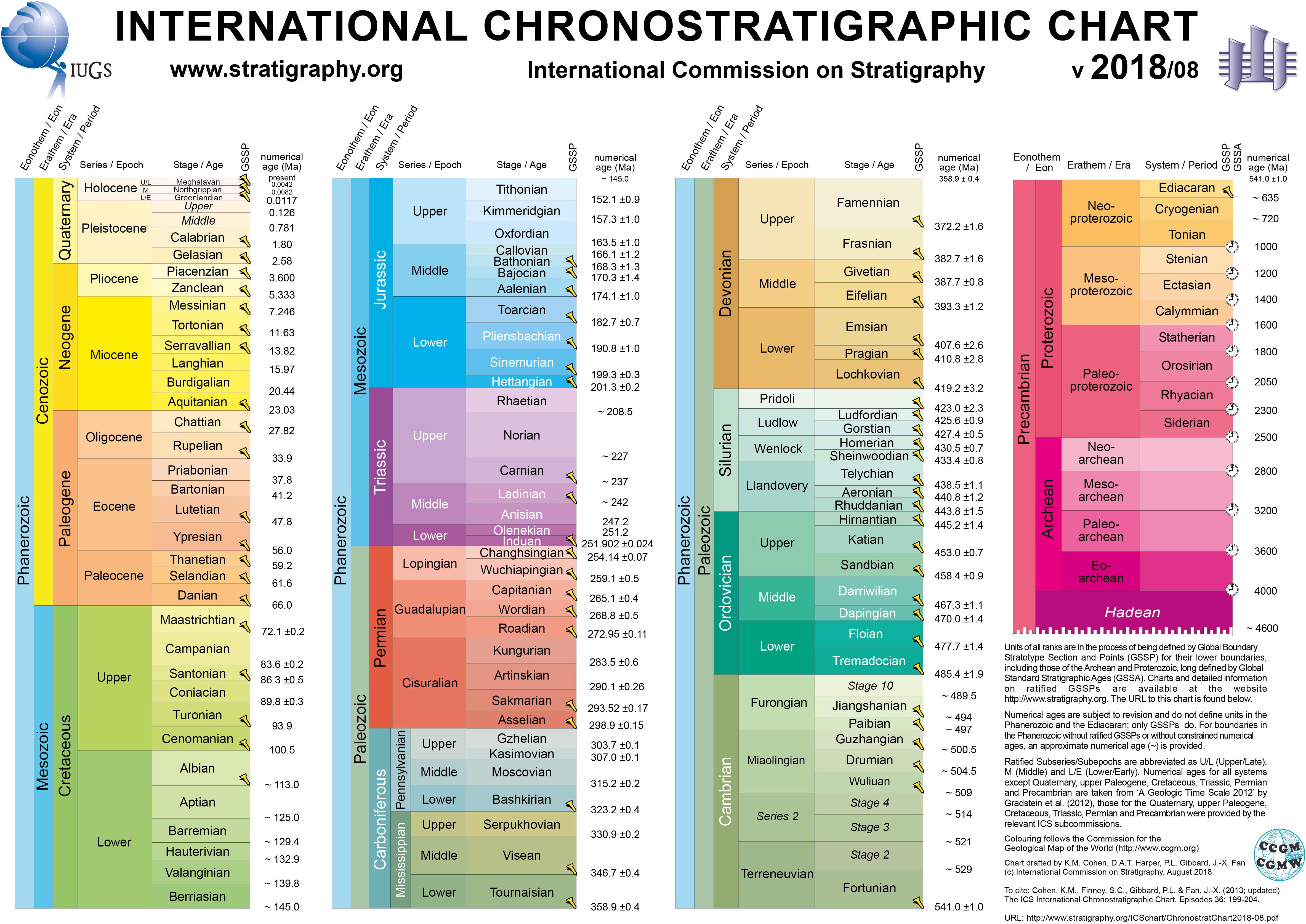
FIGURE 1. The International Chronostratigraphic Chart of the ICS in its 2018 online version (Cohen et al., 2018, www.stratigraphy.org).
The chronostratigraphic scale has been under construction for more than 200 years. Since 1961, the International Commission on Stratigraphy has taken control of developing and standardizing the chronostratigraphic scale through the definition of chronostratigraphic boundaries by Global Stratotype Sections and Points (GSSPs). Since early objections to this method were swept aside in the 1960s and 1970s, the philosophy and methodology of GSSP-based chronostratigraphy has not been seriously questioned in print. Here, I first review in brief the history, philosophy and methods by which the chronostratigraphic scale has been developed. I then summarize the current status of the GSSP-based chronostratigraphic scale. I follow with a critique of the GSSP-based chronostratigraphy, both its underlying philosophy and much of its methodology.
I thereby demonstrate that the GSSP method has produced a chronostratigraphic scale (Figure 1) fraught with problems of philosophy and methodology. I conclude by arguing that the way forward with chronostratigraphy is a return to the concepts of natural chronostratigraphy, with improvements based on modern techniques like quantitative biostratigraphy. We need to standardize the chronostratigraphic scale by rethinking the philosophy and practices by which this is being done, so that we can produce the most informative chronostratigraphy possible based on a consistent methodology that allows the updating and obtaining of high accuracy and precision as new data become available.
Some Terminology, Acronyms and Scope
Much of the literature on stratigraphic theory and practice is concerned with terminology or what is more dismissively referred to as semantics. In reviewing much of that literature, I am reminded of a quip by the famous sedimentologist Paul Krynine (1902–1964), who said that stratigraphy represents the “complete triumph of terminology over facts and common sense” (cf. Folk and Ferm, 1966, p. 853). I do not want to become mired in semantics here. Thus, I accept readily the current hierarchy of chronostratigraphic units as (smallest to largest) stages, series, systems, erathems and eonothems (e.g., Hedberg, 1976; Salvador, 1994; Aubry et al., 1999). Definitions given of a few common words used here are those of standard English-language dictionaries.
In this article, GSSP is Global Stratotype Section and Point, and ICS is the International Commission on Stratigraphy of the International Union of Geological Sciences. I make an important distinction between biostratigraphic datums and biochronological events (e. g., Williams, 1901; Teichert, 1958; Berggren and van Couvering, 1978; Murphy, 1994; Remane, 2003; Gradstein, 2012). Biostratigraphic datums are the lowest occurrence (LO) and highest occurrence (HO) of a fossil in a stratigraphic section. Biochronological events are the first appearance datum (FAD) and last appearance datum (LAD) of a taxon, ideally its evolutionary origination and extinction, respectively. However, immigration, emigration, local or regional extirpation and abundance acme can also be significant biotic events of value to biostratigraphy and biochronology. For chronostratigraphic definition, it is hoped that the LO and the FAD of a taxon coincide, at least if the LO is the primary signal for correlation of a GSSP. However, given the problems of sampling, facies and provinciality, it is highly unlikely that this will ever be the case.
My focus here is on the Phanerozoic chronostratigraphic scale. The older part of the geological timescale (Precambrian) is generally lacking or depauperate in fossils, so Precambrian chronostratigraphic boundaries have been defined by numerical ages, not by events, though this practice has been called into question (e.g., Bleeker, 2004a,b; Van Kranendonk et al., 2012). This is not true of the last part of Proterozoic time, the Ediacaran, and it should be possible to define earlier parts of the Precambrian by biotic/physical events as well. However, my discussion limits itself to the Phanerozoic.
The Taxonomy of Time
A standard definition of chronostratigraphy is that it is that part of stratigraphy “that deals with the relative time relations and ages of rock bodies” (Salvador, 1994, p. 113). I think it is also fair to regard chronostratigraphy as very much about the taxonomy and classification of geological time. Simpson (1961), p. 11) wrote that “taxonomy is the theoretical study of classification, including its bases, principles, procedures, and rules.” He was writing about zoological taxonomy, but I believe his is a general definition of taxonomy that can also be applied to chronostratigraphy. The chronostratigraphic scale is a hierarchical classification. Simpson (1961, p. 13) described such a hierarchical classification as a “sequence of classes (or sets) at different levels in which each class except the lowest includes one or more subordinate classes.” Simpson (1961, p. 25) also concluded that “some classifications pertain to a wider range of inductions or to more meaningful generalizations than others and are in that sense ‘better,’ or more useful.” Thus, classifications that impart more information are more useful (“better”) than those that impart less information.
Some History
Geologists have devoted more than 200 years to developing the chronostratigraphic scale. The history of this development is long and complex and has been the subject of book-length treatments (e.g., Albritton, 1986; Berry, 1987a), is reviewed in diverse ways in timescale compendia of the last 30–40 years (Harland et al., 1982, 1990; Gradstein et al., 2004a, 2012), is discussed in some textbooks on stratigraphy (e.g., Gignoux, 1955; Dunbar and Rodgers, 1958) and is the subject of too many scientific articles to list here. Furthermore, an extensive literature on the theory and practice of chronostratigraphy and related topics exists, mostly in scientific journal articles. Thus, my treatment of the history of chronostratigraphy is necessarily brief. In so doing, I divide it into three phases: (1) Geognosy; (2) Natural chronostratigraphy; and (3) GSSP chronostratigraphy.
Geognosy
The first attempts at broad subdivision of the stratigraphic record were based on lithology. German mining geologists of the 1700s, most famously Abraham Werner (1750–1817), divided the stratigraphic record into a simple succession of distinct lithosomes. The most lasting of these “geognostic” efforts was the classification of the Italian Giovanni Arduino (1760), who, in 1760, recognized three classes of mountain-forming rocks: Primitive, Secondary and Tertiary. The latter term was part of the chronostratigraphic scale until relatively recently (see Wilmarth, 1925, p. 49, for an accessible translation of Arduino on the Tertiary).
This geognostic method produced very coarse stratigraphic subdivisions that could only be recognized in small areas because of the lateral variability and time transgression of lithofacies. Geologists have long known that subdivisions of the stratigraphic record based on lithology alone are almost always very local in extent and are the practice of lithostratigraphy, not chronostratigraphy.
Natural Chronostratigraphy
By about 1800, the use of fossils to organize stratified rocks began with William Smith (1769–1839) in England and Georges Cuvier (1769–1832) and Alexander Brongniart (1770–1847) in France. Thus, as Smith observed, “the same strata were found always in the same order of superposition and contained the same fossils” (attributed to Smith by Arkell, 1933, p. 5). The underlying concept was well captured by Murchison (1839, p. 9), who wrote “the zoological contents of rocks, when coupled with their order of superposition, are the only safe criteria of their age.” Thus, the presence of and stratigraphic succession of different kinds of fossils came to underpin chronostratigraphic classification, and time intervals like Murchison’s Silurian were characterized primarily by the fossil content of the rocks that were thought to have been deposited during that time interval.
From Alcide d’Orbigny (1802–1857) came the concepts stages and zones, followed by their initial and detailed development by the field efforts of Friedrich Quenstedt (1809–1889) and Albert Oppel (1832–1865) using Jurassic ammonoids. Through these and similar works, by the second half of the 1800s, the concept of biotic (faunal) succession was well established (e.g., Arkell, 1933; Monty, 1968; Rudwick, 1996). Indeed, in 1855, Charles Lyell first published a hierarchical chronostratigraphy based on fossil succession (Figure 2).
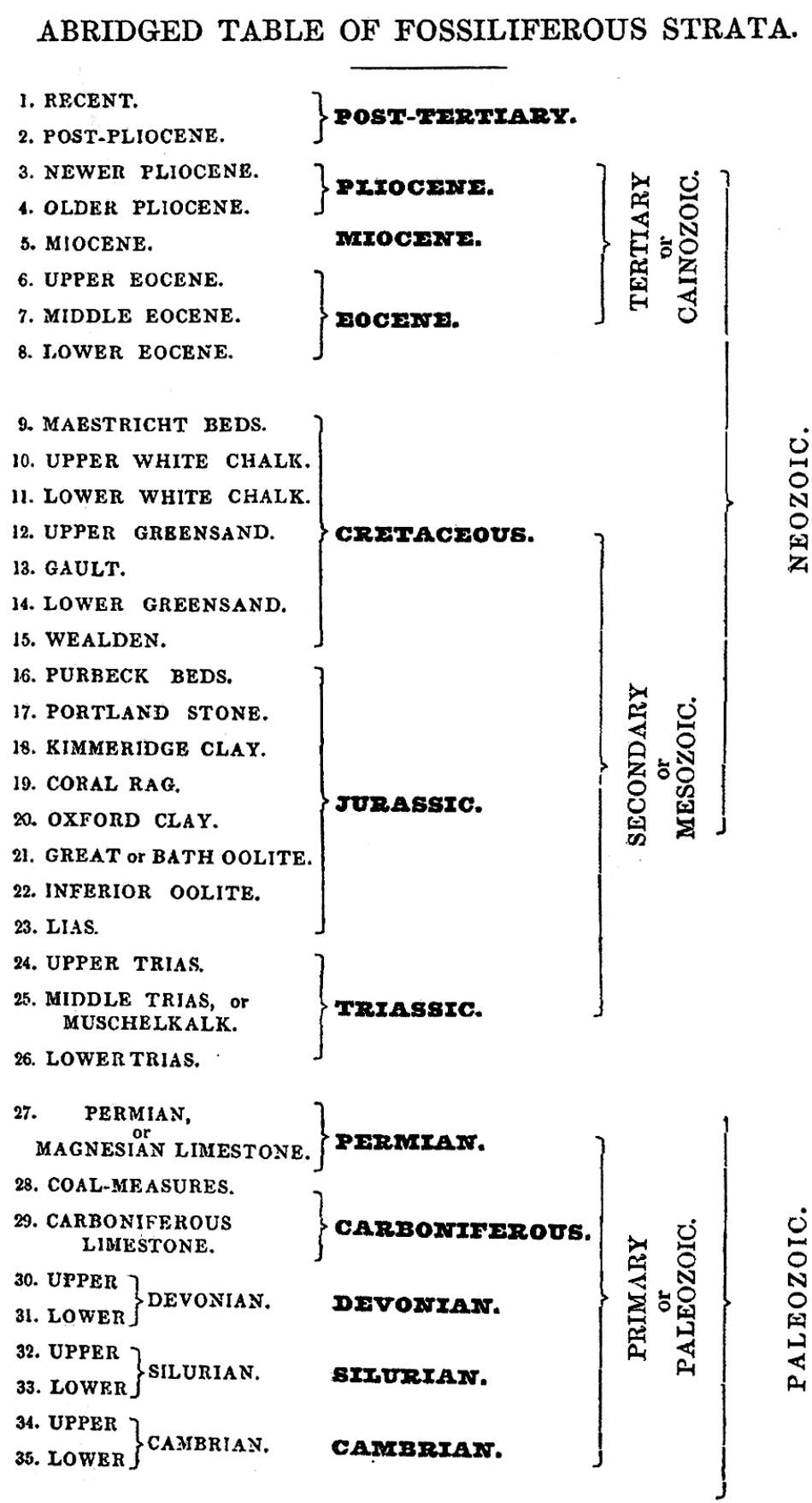
FIGURE 2. The chronostratigraphic chart of Lyell (1855, p. 109), an “abridged table of fossiliferous strata.” According to Head et al. (2017, p. 4), “probably the first-ever multi-hierarchical chronostratigraphic chart.” Reproduced by kind permission of the Syndics of Cambridge University Library.
One of the key ideas that had its roots in the “catastrophism” of Cuvier, D’Orbigny and others was that substantial breaks/changes could be used to identify the boundaries between intervals of geologic time. Using such breaks would produce what came to be called natural classifications of geological time. As a good example of such a natural classification, British geologist Phillips (1860, Figure 4) used major drops in diversity (extinctions) to delimit the Paleozoic, Mesozoic and Cenozoic, still recognized as the erathems of the Phanerozoic Eonothem (Figure 3).
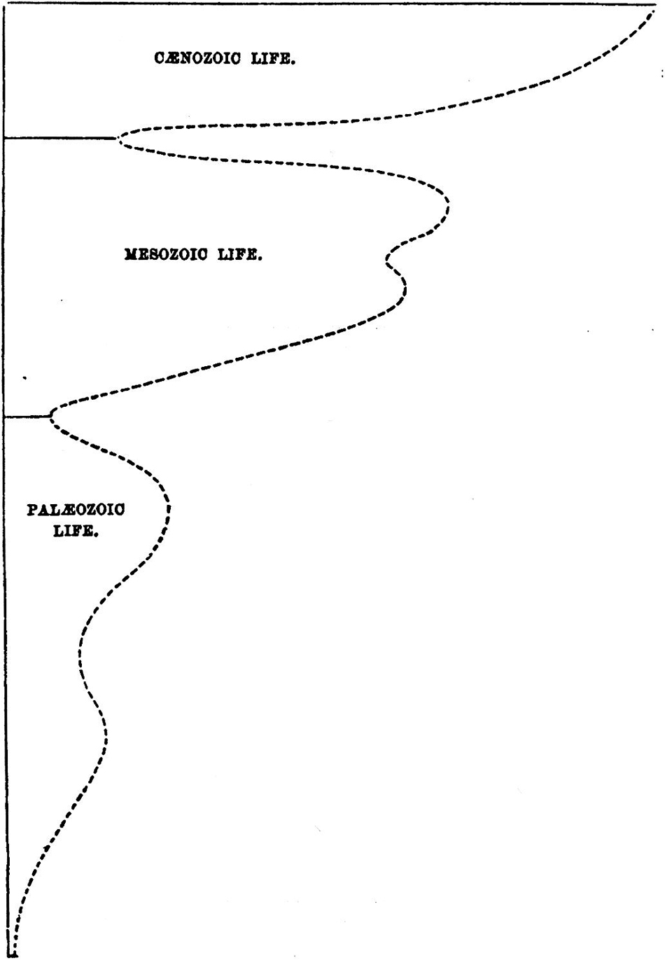
FIGURE 3. Phillips (1860, p. 66; Figure 4) diagram that shows his basis for recognition of the Paleozoic, Mesozoic and Cenozoic eras, “which corresponds to the numerical prevalence of life and represents its rise and fall.”
Another aspect of such breaks was the idea (most famously articulated by Chamberlin, 1909) that the earth had experienced a succession of orogenic events (“diastrophism”) that produced periodic global events recorded by the stratigraphic record. As one of many examples, consider a lengthy article by the famous Kansas stratigrapher Moore (1940) identifying and correlating unconformities to position the Carboniferous-Permian boundary. The idea that the base of each geological system should be an unconformity did not essentially die until Gilluly (1949) convincingly argued that there were no such global episodes of orogeny, though unconformities of eustatic origin continue to play a role in some chronostratigraphic definitions.
By the 1950s, it was well accepted that the boundaries of series, systems, erathems and even the base of the Phanerozoic Eonothem were marked by significant events–biotic and/or physical–that identified natural junctures that could be used to create a chronostratigraphic classification. As Newell (1966, p. 80) put it, “conspicuous world events, such as mass extinctions…provide natural datums for the division of chapters of earth history and should be stressed in standard stratigraphic classification.” The problems of hiatuses between boundaries, the time transgressive nature of boundaries and the temporal overlap of many named chronostratigraphic units (particularly stages) were well understood (see, for example, Wheeler and Beesley, 1948). But, it is fair to say that the chronostratigraphic scale by the 1950s was a classification of geologic time based on using what most called “natural” events as the basis for subdivision.
Nevertheless, as is the case with any taxonomy, there were disagreements that led, in many cases, to a lack of uniformity in the subdivision of geological time. Thus, from the beginning of natural chronostratigraphy there were debates over what events to use to place boundaries and disagreements about the ranks and the names of chronostratigraphic units. Indeed, such debates were nearly as old as natural chronostratigraphy itself, starting in the 1830s with the famous Cambrian-Silurian controversy of Adam Sedgwick and Roderick Murchison.
GSSP Chronostratigraphy
During the last century, after World War II, a new approach to chronostratigraphy developed that I call GSSP chronostratigraphy. It was part of a laudable movement to standardize global chronostratigraphy. The GSSP method embodied radical changes from the previous process of chronostratigraphic definition. Indeed, its underlying philosophy was a fundamental departure from previous thinking on how to divide geologic time.
Hedberg (1903–1988), who was a key figure in the creation of the ICS, proved to be instrumental in the philosophy that underlies the GSSP method. In his writings, Hedberg (1948, 1951, 1958, 1968, 1976; Hedberg, 1965a,b) revealed himself to be both a gradualist and reductionist, who thought that any boundaries of geological time can be chosen arbitrarily. Thus, Hedberg (1948, p. 447) stated that “paleontological evidence of time in rocks is always imperfect” and that with regard to large scale chronostratigraphic subdivisions (systems and series) “it is doubtful that their division points are marked by ‘natural breaks’ in the fossil record.”
Hedberg (1968, p. 193) also advocated the recognition of “one single set of standard world-wide stages,” though he did recognize the ongoing utility of regional stages. Furthermore, he emphasized the need for type sections of chronostratigraphic units. Initially, these were the unit stratotypes of previous practice, but after British stratigraphers advocated the concept of boundary stratotypes, Hedberg (1965a, et seq.) endorsed that concept.
However, unlike many who followed, Hedberg (1965a, p. 104) advocated an eclectic approach based on the boundary stratotype, stating that it has several advantages that include “it allows those who believe in ‘natural’ worldwide divisions of Earth history opportunity to influence the choice of type boundaries at what, in their opinion, are the most significant horizons while still leaving others free to consider system boundaries as only useful but rather arbitrary reference markers in a continuous record of diverse geological events.” By the 1980s, boundary stratotypes came to be called GSSPs, and were also referred to as “golden spikes,” symbolically placed in a section to mark a chronostratigraphic boundary (Cowie, 1986; Cowie et al., 1986).
The underlying philosophy of GSSP chronostratigraphy embodies the concept that geological time can be divided arbitrarily, not at so-called “natural” breaks, and that what we need to do is simply define a chronostratigraphy with GSSPs to achieve a stable, precise and useful chronostratigraphy. GSSP chronostratigraphy thus grew out of a desire to have a single, standardized global chronostratigraphy and was also at least in part a reaction to the many disagreements and the hiatus-based boundaries that had long beleaguered natural chronostratigraphy.
The GSSP Method
The GSSP method is explained in detail elsewhere (e. g., Hedberg, 1976; Cowie, 1986; Cowie et al., 1986; Salvador, 1994; Remane et al., 1996; Gradstein et al., 2003, 2004c; Smith et al., 2014; Finney and Edwards, 2016), obviating the need for a detailed explanation here. And, an extensive literature justifies it philosophically and methodologically (see, for example, Gradstein et al., 2004b and Smith et al., 2014 and references cited therein).
In brief, the GSSP is a point (stratigraphic level) in a specific location (stratigraphic section) that defines the base of a stage (Figure 4). The GSSP is correlated by a primary signal, usually a biostratigraphic datum, and by secondary signals—biostratigraphic, chemostratigraphic, magnetostratigraphic, and radioisotopic, among others. The GSSP is not placed at an unconformity or at a lithologic change, so it is at a stratigraphic level of “continuous” sedimentation. As Ager (1981, p. 77) wrote, the GSSP “should be chosen in a section where sedimentation seems to have been nearly as continuous as is ever possible, where there are no marked lithological changes and where there are unbroken records of several different groups of fossils.”
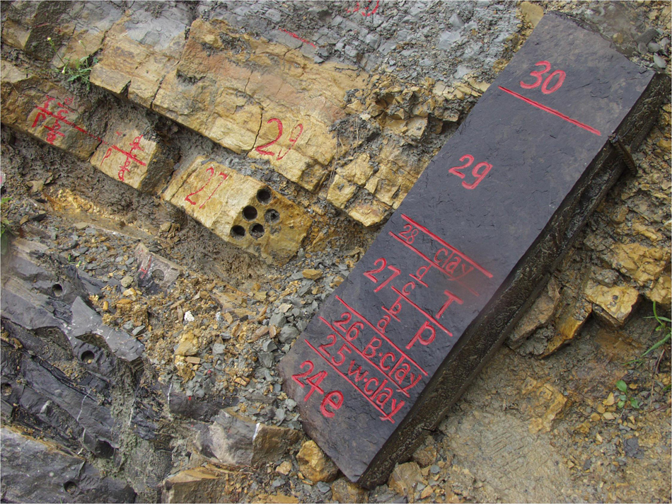
FIGURE 4. The GSSP point for the base of the Induan Stage (=base of Triassic, =base of Mesozoic) at Meishan in southern China. As the tablet on the right of the photograph indicates, the GSSP for the base of the Triassic is the base of bed 27c. Photograph courtesy of Shuzhong Shen.
The primary signal of a GSSP should be correlateable over a broad area, and there should be secondary signals (proxies) to support that correlation and that may provide correlation to places where the primary signal is absent (Finney, 2013). The GSSP of the base of a stage by default defines the bases of larger chronostratigraphic units (series, systems, erathems and eonothems) that have that stage at their base. Thus, the base of the Fortunian stage defines the bases of the Terreneuvian Series, Cambrian System, Paleozoic Erathem and Phanerozoic Eonothem (Figure 1).
The choice, evaluation and placement of GSSPs is overseen by the ICS and its subcommissions devoted to the chronostratigraphic systems. A working group (also called a task group) of an ICS subcommission is formed to identify candidate sections and criteria for GSSP selection. The criteria are the signals by which the GSSP will be correlated. After the alternative sections and criteria are reviewed, the working group votes followed by voting by the members of the relevant subcommission and up the line through the ICS structure (Figure 5).
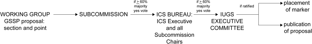
FIGURE 5. Flow chart showing how the ICS votes on and ratifies a GSSP (redrawn after Finney and Edwards, 2016; used with the permission of the copyright holder, The Lethaia Foundation, Published by John Wiley & Sons Ltd.).
The GSSP-Defined Phanerozoic Chronostratigraphic Scale
As of September 2018, the ICS recognized 102 Phanerozoic stages and on its chart showed 71 ratified GSSPs (Figure 1). Thus, about two-thirds of the Phanerozoic stage bases now have ratified GSSPs after almost 60 years of work. Here, I briefly review the status of the Phanerozoic chronostratigraphic scale defined by the GSSPs of the bases of stages. My review also draws attention to some of the obvious inconsistences and problems that have beset the development of a GSSP-based Phanerozoic chronostratigraphy.
Cambrian
The Cambrian Subcommission divides the Cambrian into four series and 10 stages. Four intra-Cambrian GSSPs have been ratified—the bases of the Drumian, Guzhangian, Paibian, and Jiangshanian stages (Figure 1). All of these GSSPs have primary signals that are the LOs of “cosmopolitan” agnostoid trilobites, and are associated with secondary signals based on other trilobite bioevents and carbon-isotope stratigraphy (Peng et al., 2012). The remaining undefined GSSPs will also likely have primary signals based on trilobite biotic events, except for the second stage (the unnamed post-Fortunian stage), which may have a primary signal based on small shelly fossils or archaeocyathans (Peng et al., 2012, Table 19.1).
The Cambrian Subcommission created a working group on the Precambrian-Cambrian boundary in 1972. Three possible Cambrian bases were advocated, the classic criteria–LO of small shelly fossils or LO of trilobites–and a trace fossil LO (Cowie, 1981). The working group initially advocated the LO of diverse shelly fossils with good correlation potential as the likely signal. However, such shelly fossils were shown to have marked provincialism as well as restriction to carbonate facies. Similarly, Brasier (1989, p. 120) noted that “the appearance of trilobites was a facies-controlled, diachronous biomineralization event.” However, instead of identifying the LOs most likely to approximate the FADs of these classic criteria by which the base of the Cambrian had long been defined, the focus switched to looking at trace fossils for boundary definition (Alpert, 1979; Crimes, 1989). This, despite the fact that trace fossils are well known to be facies controlled, so that they have never had substantial biostratigraphic utility.
Ultimately, a basal Cambrian GSSP was ratified in 1992 for a section in Newfoundland, Canada, with the primary signal of the GSSP the LO of the trace fossil taxon Treptichnus (= Trichophycus) pedum (e.g., Brasier et al., 1994). But, less than a decade after ratification of the GSSP, Gehling et al. (2001) reported that at the GSSP location the stratigraphic range of T. pedum was extended about 3–4 m lower than the GSSP level. Thus, the GSSP for the base of the Cambrian needs to be redefined.
The Cambrian Subcommission also took the unusual step of naming new series and stages for the global standard stages, not using longstanding names such as Tommotian and Acadian. This was done to avoid the “baggage” associated with the older stage names (e.g., Peng and Babcock, 2011).
Ordovician
The Ordovician Subcommission has defined the bases of all seven Ordovician stages (assigned to three series) with ratified GSSPs (Cooper et al., 2012). The primary signals of the bases of two stages, Tremadocian (=base of Ordovician) and Dapingian, are conodont biotic events, but the other GSSPs have graptolite biotic events as their primary signals. However, Cooper et al. (2012, p. 490) noted that “because of marked faunal provincialism and facies differentiation throughout most of the Ordovician, no existing regional suite of stages or series has been found to be satisfactory in its entirety for global application.” Indeed, for example, the GSSP-defined chronostratigraphy of the Ordovician is of little use in correlating Midcontinent North American Ordovician marine strata (e g., Witzke, 2013).
Like the Cambrian Subcommission, the Ordovician Subcommission has generally introduced new stage names. However, they have not been consistent in this, also using some older names, such as Tremadocian (a very old British term that dates to Sedgwick in the 1840s) and Dariwillian (an Australian stage name coined in 1899).
Silurian
The Silurian is divided into eight stages grouped in three series (though Pridolian is treated as both a series and a stage) (Melchin et al., 2012). The Subcommission on Silurian Stratigraphy has approved the GSSPs of all the Silurian stage bases, all with primary signals at the bases of standard graptolite zones (Melchin et al., 2012).
The Ordovician-Silurian boundary working group began in 1976. It ratified a GSSP at Dob’s Lin in Scotland in 1984 with the primary signal of the base of the Silurian the LOs of the graptolites Akidograptus ascensus and Palakidograptus acuminatus. However, this GSSP (base of the Rhuddanian Stage) was objected to early on both procedural grounds and as not corresponding to the “best” level in the graptolite succession (Berry, 1987b; Lespérance et al., 1987).
Indeed, in 2000 the Silurian Subcommission decided to re-examine the base of the Silurian, as well as the base of the Sheinwoodian Stage, which is the base of the Wenlock Series (Melchin et al., 2012) The bases of the Aeronian and Ludfordian have also been shown to be problematic. Thus far, the base of the Silurian GSSP has been changed to a different stratigraphic level in the same GSSP section (Rong et al., 2008), but the other problematic Silurian GSSPs await resolution.
Devonian
The Subcommission on Devonian Stratigraphy divides the Devonian into seven stages grouped in three series (e.g., Ziegler and Klapper, 1985). The GSSPs of the bases of all Devonian stages have been ratified and have conodont biotic events as primary signals, except for the base of the Devonian, which has a primary signal based on graptolites. However, revisions of the bases of the Emsian and Pragian stages are needed because of problems correlating their primary signals (Becker et al., 2012).
In 1960, the IUGS created a committee to study the Silurian-Devonian boundary, and a GSSP was designated in 1972 at Klonk in the Czech Republic, with its primary signal the LO of the graptolite Monograptus uniformis. This was the first ratified GSSP and has long been held up as a model of how well the GSSP method works (e.g., Chulpáč and Vacek, 2003). Indeed, Cowie et al. (1986) stated that “much inspiration and guidance has been derived…from the brilliantly expressed published results of the Silurian-Devonian Boundary Committee (McLaren, 1977).”
Carboniferous
The Carboniferous is divided into seven stages grouped in three series (Davydov et al., 2012). In 2004, the Carboniferous Subcommission adopted the Mississippian and Pennsylvanian as “subsystems” of the Carboniferous System (Heckel and Clayton, 2006). Three Carboniferous GSSPs have been ratified, the bases of the Tournaisian (=base of Carboniferous), Visean and Bashkirian stages. The primary signals of the base of the Tournaisian and Bashkirian are conodont biotic events, whereas the primary signal of the base of the Visean is a foraminiferal event. However, the primary signal of the base of the Tournaisian is a conodont event (LO of Siphonodella sulcata) that has been found stratigraphically lower in the GSSP section at La Serre, France, so this GSSP is being redefined (Kaiser and Corradini, 2008; Kaiser, 2009). And, the base of the Bashkirian (=base of Pennsylvanian) is in a stratigraphic section riddled with unconformities and may need to be relocated (Smith et al., 2014).
Permian
The Subcommission on Permian Stratigraphy recognizes a Permian chronostratigraphic scale of nine stages in three series (Lucas and Shen, 2018). GSSPs for the bases of six of the stages have been ratified with conodont biotic events as their primary signals. Work to define formally the three remaining stages bases, with conodonts as primary signals, is well underway.
There are, nevertheless, problems related to the ratified Permian GSSPs that include:
(1) Rarity and possible diachroneity of the primary signal of the base of the Asselian Stage (=base of Permian), the LO of the conodont Streptognathodus isolatus (Lucas, 2013).
(2) Temporal overlap of the Guadalupian and Lopingian Series based on recent ammonite biostratigraphy (Zhou, 2017).
(3) Conodont-based primary signals of the three Guadalupian stages at their GSSP locations in West Texas are either elusive or stratigraphically below their defined GSSP levels (Shen, personal communication, 2017).
(4) The provinciality of Guadalupian and Lopingian conodonts (Mei and Henderson, 2001) renders problematic the global correlation of the conodont-based primary signals of the relevant stage GSSPs.
Triassic
The Subcommission on Triassic Stratigraphy recognizes seven Triassic stages arranged in three series. At present, only three Triassic GSSPs have been ratified: base of Induan (=base of Triassic), Ladinian and Carnian stages (Lucas, 2010). The latter two have ammonoid biotic events as their primary signals, and the base of the Induan has a conodont event as its primary signal. However, this conodont signal, the LO of Hindeodus parvus at the Meishan GSSP in south China (Figure 4), is now known to be a relatively young occurrence of this taxon. Thus, the primary signal to correlate the base of the Triassic is diachronous (Jiang et al., 2011; Brosse et al., 2015), though no effort to redefine the GSSP has begun.
In 2007, the working group of the STS voted to favor (though not by a significant majority) a basal Olenekian GSSP in India with its primary signal the LO of the conodont Neospathodus waageni. Not long after the vote, N. waageni was found to have older occurrences at the proposed GSSP section than previously known, derailing the effort to define this GSSP (Zakharov, 2010). And, for more than a decade, the LO of the conodont Chiosella timorensis at the Deşli Caira section in Romania had been considered the potential primary signal for a base Anisian GSSP (e.g., Orchard et al., 2007). However, discovery of that species in late Spathian strata (Goudemand et al., 2012) extended its stratigraphic range and derailed definition of a basal Anisian GSSP.
Similarly, Krystyn et al. (2007) proposed to define a GSSP for the Rhaetian base at Steinbergkogel in Austria. The working group voted on the GSSP level, and a majority chose the level with the LO of the conodont Misikella posthernsteini as its primary signal (Krystyn, 2010) (Figure 6). However, Giordano et al. (2010) concluded that the LO of Misikella posthernsteini is actually younger at Steinbergkogel than it is in the section they studied in the Lagonegro basin in southern Italy. Thus, the LO of M. posthernsteini at Steinbergkogel is not the FAD of the species.
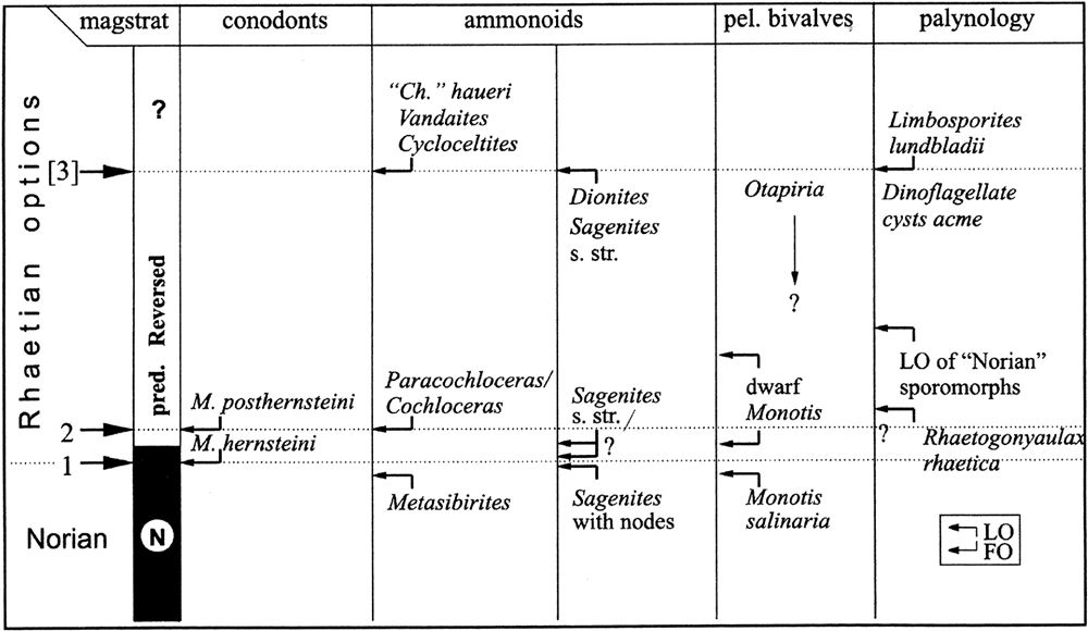
FIGURE 6. The signals associated with the proposed GSSP of the base of the Rhaetian Stage at Steinbergkogel in Austria (after Krystyn et al., 2007). Note that FO, first occurrence and LO, last occurrence.
Attempts to use conodonts as primary signals of Triassic GSSPs thus have been problematic and have delayed definition of some of the Triassic GSSPs for decades (Lucas, 2016). At present, efforts are underway again to define base Olenekian and Rhaetian GSSPs using conodont signals.
Jurassic
The Jurassic Subcommission recognizes 11 stages organized into three series. The GSSPs of seven of these stages have been ratified, including the base of the Hettangian, which is the base of the Jurassic (Ogg et al., 2012b; von Hillebrandt et al., 2013). All of these GSSPs have ammonite bioevents as primary signals.
In 2010, a section at Kuhjoch, Austria, became the GSSP for the base of the Jurassic, even though nothing had been published on this section until the actual GSSP proposal (von Hillebrandt et al., 2007). We now know that this little studied section was poorly chosen, as the section is tectonized (Palotai et al., 2017), which is contrary to one of the requirements for a GSSP section (Remane et al., 1996). The GSSP for the base of the Jurassic thus needs to be relocated.
Cretaceous
The Cretaceous Subcommission recognizes 12 stages organized into two series. The bases of five stages have ratified GSSPs (Ogg et al., 2012a; Lamolda et al., 2014; Kennedy et al., 2017), either with primary signals based on planktonic foraminiferans (Albian, Cenomanian, Santonian), inoceramid bivalves (Santonian) or ammonites (Turonian).
Despite decades of effort (cf. Remane, 1991), there still is no agreed on GSSP for the base of the Berriasian Stage, which is the base of the Cretaceous. For convenience, a magnetostratigraphic marker (base of Chron M18r) has long been used for the Cretaceous base. Ogg et al. (2012a, Figure 27.2) reviewed this issue at some length, showing 13 potential signals to correlate a base Cretaceous GSSP. Their explanation of the delay is the “lack of any major faunal change between the latest Jurassic and earliest Cretaceous, pronounced provincialism…and of persistent debates on which stratigraphic marker might provide the most useful global correlation levels” (Ogg et al., 2012a, p. 795).
Paleogene
The Paleogene Subcommission recognizes nine stages grouped in three series (Vandenberghe et al., 2012). The GSSPs of seven of the stage bases have been ratified. Unlike the older Phanerozoic stage GSSPs, non-biostratigraphic events are the primary signals of some of the Paleogene GSSPs. Thus, the base of the Danian (=base of Paleocene, base of Paleogene, base of Cenozoic) has the iridium-rich clay layer from the Chicxulub bolide impact as its primary signal, the Thanetian base GSSP is at the base of magnetochron C26N and the base of the Ypresian stage (=base of Eocene) has a carbon-isotope excursion as its primary signal. The bases of the Selandian and Lutetian have calcareous nannoplankton events as primary signals. And, the base of the Rupelian has the extinction of the foraminiferal family Hantkeninidae as its primary signal, which is the only extinction event used as the primary signal of a GSSP, and looks to be problematic (Pearson et al., 2008). Recognition of and a push to formalize “subseries” (a new level of the chronostratigraphic hierarchy) such as “middle Eocene” is an ongoing effort of the Paleogene Subcommission (Head et al., 2017).
Neogene
The Neogene Subcommission recognizes eight stages in two series, and six of the stages have ratified GSSPs (Hilgen et al., 2012). Like the Paleogene, some of these GSSPs have non-biotic primary signals. In particular, a precessional excursion of the astronomically tuned time scale has been used as the primary signal of the base of the Piacenzian. The base of the Aquitanian (=base of Neogene, =base of Miocene) is at a magnetochron base, and an isotope excursion marks the base of the Servalian. The GSSP of the base of the Zanclean is located at an insolation cycle but may be at an unconformity and in need of re-evaluation (Smith et al., 2014). Foraminiferal and nannoplankton biotic events are the primary signals of the bases of the Tortonian and Messinian.
Quaternary
For decades, culminated by Berggren (1998), various arguments were advanced to abandon the term Quaternary, and Berggren further advocated abandoning the Tertiary. The debate that ensued was resolved by a combined nomenclature in which the Cenozoic Erathem is divided into three systems: Paleogene (Paleocene, Eocene + Oliogocene), Neogene (Miocene + Pliocene) and Quaternary (Pleistocene + Holocene) (Gibbard et al., 2010). Tertiary, the last remnant of the geognostic scale, is gone (at least for now!).
The redefined Quaternary consists of two series, Pleistocene and Holocene, and the former is divided into four stages (Figure 1). Three GSSPs have been ratified (Pillans and Gibbard, 2012). The base of the Gelasian Stage is at a precessional excursion. The base of the Calabrian Stage is a claystone bed said to be ∼15 kyr younger than the end of the Olduvai normal polarity chron, and the base of the Tarrantian is the base of Isotope Stage 5e that corresponds to the end of the younger Dryas stadial. The base of the Holocene is at a stratigraphic level in an ice core from Greenland.
Three new Holocene stages were just ratified by ICS—Greenlandian, Northgrippian and Megalahayan. The primary signal of the base of the Megalahayan—a supposed global drought 4200 years ago—has already been challenged (Voosen, 2018). The naming of the Megalahayan may also obviate the need to recognize the much discussed Anthropocene Stage (e.g., Waters et al., 2014).
Problems With the Approach and Method of GSSP Chronostratigraphy
There has been much disagreement about individual GSSPs, particularly regarding their geographic locations, stratigraphic levels and signals. Indeed, some of these disagreements have lasted for decades (see the quote above regarding the base of the Cretaceous). However, objections to the philosophy and method underlying the GSSP method have been few and are mostly found in an older literature of the 1960s and 1970s (e.g., Newell, 1966; Meyen, 1976; Krassilov, 1978) that was long ago swept aside by the GSSP method proponents, such as McLaren (1970, 1977) and Ager (1981, 1984). Notably, the GSSP method found little acceptance among Soviet (Russian) stratigraphers (e.g., Gladenkov, 2014). Here, I question several aspects of the underlying philosophy and the methods of GSSP-based chronostratigraphy.
Inconsistency
The brief review just given of the ICS chronostratigraphic scale reveals many inconsistencies in how the ICS subcommissions have named and defined chronostratigraphic units. Thus, the Cambrian Subcommission is giving new names to the stages and series it defines, the Ordovician Subcommission is doing this in part (but still keeping some traditional names), and the other subcommissions are using existing chronostratigraphic terms. And, for the Carboniferous, we even have a new rank in the chronostratigraphic hierarchy of “subsystem” for the Mississippian and Pennsylvanian, and the Paleogene Subcommission wants another new rank, the “subseries.”
Methodologically, it is clear that diverse criteria have been chosen as the primary signals of GSSPs. Clearly, not all ICS factotums agree that an arbitrarily chosen signal, such as an arbitrary point in a hypothetical conodont chronomorphocline (see below), should be the primary signal of a GSSP. There are many Paleozoic GSSPs for which such “arbitrary” points in hypothetical conodont phylogenies are the GSSP signal, but other biotic events are not so arbitrarily chosen. One is the extinction of the foraminiferal family Hantkeninidae that marks the base of the Rupelian Stage (= base of the Oligocene Series).
Furthermore, other kinds of signals have been used as the primary signal of many GSSPs that are non-biotic and that are inherently not able to be uniquely identified without other (usually biotic) criteria. These are the base of magnetochrons, isotopic excursions, and precessional cycles of the Milankovitch spectrum, among others. Given that these signals need other closely associated signals to identify them, how can they be considered primary signals? Indeed, how does one use precessional excursion 347 from the present (the primary signal of the GSSP that defines the base of the Pliocene) to correlate that signal in most facies? Instead, such signals should be secondary signals.
If the goal of the ICS is to produce a single, standardized global chronostratigraphy, why such inconsistencies? Some of the inconsistencies, of course, are the results of having 12 different subcommissions focus on the different systems of the Phanerozoic chronostratigraphic scale. The different systems offer varied signals by which to correlate GSSPs. Thus, the inconsistencies reflect the differing philosophies, methods, priorities and available data of the different subcommissions. They also reflect a failure by the ICS to standardize both terminology and methodology. Thus, there has been no consistent method of GSSP definition (beyond the bureaucratic aspects outlined in Figure 5), so the ICS chronostratigraphy is not standardized.
Arbitrary Decisions
Arbitrary decisions are random, based on personal choice or whim and thus are not based on any system or line of reasoning. Therefore, arbitrary decisions are not scientific decisions. Nevertheless, our psychological perception of time is of something that flows continuously, like water in a river. From this comes the argument that time, by itself, can only be divided arbitrarily (e.g., Kitts, 1966, 1989). In other words, time, as a continuously and uniformly (relatively speaking) flowing entity provides no non-arbitrary signals by which we can divide it into intervals. The signals that we use to divide time are events to which we attribute some significance that are used to construct a temporal framework.
Thus, for example, we can readily divide the time interval of the 20th Century by significant events, such as the two World Wars, the assassination of John F. Kennedy, the fall of the Berlin Wall, etc. If we wanted to arbitrarily divide 20th Century time we could simply divide it into 5-year-long intervals. But, who would so divide the 20th Century and what value would there be to dividing the 20th Century arbitrarily into 5-year-long intervals? No historian would do so, simply because the resulting classification of 20th Century time would be devoid of information—it would be a meaningless classification in the sense of Simpson (1961). And, how, as scientists, can we agree on and replicate arbitrarily chosen subdivisions of time?
Nevertheless, an important underlying concept of the GSSP method has been that geological time should be divided arbitrarily. Thus, for example, Ager (1981, p. 79) argued that “it does not matter where the golden spike is hammered in…so long as we can make an arbitrary decision, stop arguing about words and get on with the much more difficult (but much more rewarding) task of correlation” (my italics). And, we find former ICS Chairman, Remane (2003, p. 12) stating that “the chronostratigraphic boundary can, however, be placed exactly within a continuous morphocline….” (But, how does one place a boundary “exactly” within something “continuous”?). Finally (and the examples could be multiplied) consider Walsh et al. (2004, p. 205), whose co-authors included then ICS Chairman Gradstein, who equated chronostratigraphic units to “classificatory pigeonholes, analogous to the arbitrarily defined grain-size pigeonholes used for classifying clastic sediments, and the arbitrarily defined compositional pigeonholes used for classifying plutonic rock” (my italics).
Generally, those who champion arbitrary chronostratigraphic boundaries decry those who want boundaries based on natural events. Ager (1984, p. 66) proved to be most derisive in this regard, referring to natural-event-based chronostratigraphy as “Marxist,” and even went on to write sarcastically that “the magic moment that was the beginning of the Devonian was ordained by God or Marx long before Man started his investigations” (Ager, 1981, p. 76). Furthermore, Ager (1984, p. 99) stated that “ultimately there are not enough big catastrophes to use as our reference points, and there are too many little ones; so, we must be arbitrary and seek only to cause the least possible confusion and inconvenience….on that basis, I cannot see any argument against our eventually switching to a purely chronometric scale.”
Well, as if to satisfy Ager’s wish, the ICS did conduct what appears to have been a very short-lived experiment in an arbitrary, chronometric scale, dividing the Precambrian numerically into (mostly) 200 million year intervals, the so-called system of Global Standard Stratigraphic Age (GSSA) (Robb et al., 2004). This, over the objections of those who knew that even a Precambrian chronostratigraphy could be event based (e. g., Cloud, 1987; Crook, 1989; Nisbett, 1991). Indeed, immediately rejected (e.g., Bleeker, 2004a,b), this arbitrary, numerical scale is being abandoned as uninformative (Van Kranendonk et al., 2012).
So, if we are to define arbitrarily the boundaries of chronostratigraphic units, how do we do this other than numerically? Some micropaleontologists, particularly those who work on conodonts, have provided a method. Thus, these micropaleontologists “know” that conodont evolution took place by gradualistic processes, many of which produce new species anagenetically (Figure 7). Weddige and Ziegler (1979; also see Ziegler and Sandberg, 1994) well explain this understanding, which had much earlier been dubbed “autochronology” by Richter (1956), Thus, “the immense stratigraphic value of conodonts that is based on phyletic gradualism, rather than on other phyletic hypotheses, is obvious in many examples from Cambrian to Triassic ages” (Weddige and Ziegler, 1979, p. 158). This view of conodont evolution is well exemplified by their analysis of the evolution of the Devonian conodont genus Polygnathus (Figure 7).
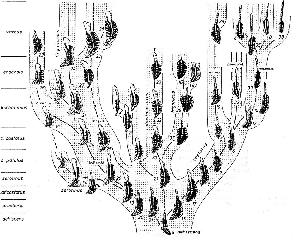
FIGURE 7. An example of the supposedly gradual and dominantly anagenetic evolution of conodonts depicted in chronomorphoclines, in this case of the Devonian genus Polygnathus (after Weddige and Ziegler, 1979; used with the permission of the copyright holder, Michael Amler, University of Cologne, Germany).
The problem is that there is no scientific rigor behind the concept that all conodont evolution took place by phyletic (largely anagenetic) gradualism. Indeed, it seems that the “corporate culture” of conodont micropaleontologists is to produce chronomorphoclines akin to “connect-the-dots art,” instead of the rigorously and metrically documented chronomorphoclines proposed in evolutionary studies of other taxonomic groups. Thus, unlike chronomorphoclines proposed in the paleontological literature for some other taxa, such as foraminiferans or fossil mammals (e.g., Hayami and Ozawa, 1975; Bookstein et al., 1978), conodont chronomorphoclines are known only from photographs/drawings of supposedly representative steps in a lineage (Figure 7). There are no data on sample sizes, no documentation of variation in samples, no metric data, indeed, none of the detailed information and analyses we should see to convince us that the data robustly support the hypothesized chronomorphocline. Indeed, the lack of any data on variation in the sample at each step in the chronomorphocline makes it an unconvincing portrayal of the evolution of the species. Instead, all we are shown is a succession of ideal morphotypes that may capture the actual chronomorphocline (Figure 7), but, without other data and analysis, the chronomorphocline must be considered incompletely documented.
Furthermore, if an arbitrarily chosen point in a conodont chronomorphocline is to be the primary signal for a GSSP (as it is for many in the Paleozoic), how is that arbitrary point actually chosen? And, can that arbitrary point be replicated by other observers? In other words, are such “arbitrary” decisions actually scientific decisions? I think not.
Reductionsim
Scientific reductionism reduces complex phenomena to the sum of their constituent parts, in order to make them easier to study. Reductionism has thus been very important to science as a way to break down complex phenomena to their components. For example, in cell biology breaking a cell down into biomolecules, or, in physics, breaking matter down to atomic and sub-atomic particles have been key to many advances (Fang and Casadevall, 2011).
The GSSP method is heavily rooted in reductionism because it has reduced each chronostratigraphic boundary to the boundary of the lowest unit in the chronostratigraphic hierarchy, the stage. This is what has been called “hierarchical reductionism,” which Dawkins (1996, p. 21) states “explains a complex entity at a particular level in the hierarchy of organization, in terms of entities only one level down the hierarchy; entities which, themselves, are likely to be complex enough to need further reducing to their own component parts, and so on.” Thus, the GSSP that defines the base of the Fortunian Stage also defines the base of the Terreneuvian Series, the base of the Cambrian System, the base of the Paleozoic Erathem and the base of the Phanerozoic Eonothem.
But, is the primary signal of the base of the Fortunian a signal significant enough to define the bases of the larger chronostratigraphic units? Those who advocate the GSSP method certainly believe it is and would argue that there is nothing inherently significant to the base of the Phanerozoic that transcends the significance of the signal (the LO of a trace fossil species) associated with the base of the Fortunian. Thinking of the famed “Cambrian explosion,” I disagree.
The GSSP method thus embodies a reductionism that trivializes the boundaries of chronostratigraphic boundaries larger than stages. Indeed, if the primary signal of the base of the Phanerozoic is the LO of a trace fossil species, what significance should be attributed to the LOs of other trace fossil species? So, we should ask why do we even continue to recognize and use chronostratigraphic divisions at the series, system, erathem and eonothem levels? Why don’t we simply have a chronostratigraphic scale that consist of the 100 or so currently recognized stages of the Phanerozoic, without grouping these stages into larger “pigeonholes?” Indeed, via the GSSP method the term Phanerozoic and its subdivisions above the stage level have no particular significance other than as successively larger “pigeonholes” within which to bin stages (cf. Walsh et al., 2004). Of course, we may continue to use the larger chronostratigraphic terms: (1) as a concession to longstanding usage (we don’t, for example, want to abandon the term Silurian, do we?); (2) given that it is convenient to have these larger groupings because the names of 12 Phanerozoic systems are more readily memorized than are the 100 stage names; and (3) these larger chronostratigraphic units are useful monikers for relatively long intervals of geologic time. But, these are reasons based on book-keeping, not on science.
I believe that the bottom up (stages) reductionism of the ICS chronostratigraphy is a mistake that has reduced the information of that chronostratigraphic classification. Series, systems, erathems and eonothems are conceptually more than just collections of stages (Aristotle: “the whole is more than the sum of its parts”). They are marked by substantial natural events such as the Cambrian explosion, the great Ordovician biodiversification event, the Devonian extinctions, etc. As was argued decades ago, particularly by Walliser (1984, 1985, 1986, 1996), those events should play a role in chronostratigraphy, as they did from about 1800 till the 1970s.
Instability
The literature on GSSPs is replete with statements that once defined, a GSSP should never be moved. As Ager (1963, p. 1046) put it, “…. the base of each stage should be regarded as fixed for all time (preferably by reference to a specified point in a type section).” In the first extensive ICS document on the GSSP method, we find Cowie (1986, p. 5) stating that the GSSP “will be expected to remain fixed in spite of discoveries stratigraphically above or below,” though Cowie (1986) had already stated exactly the reverse(!). Or, Vai (2001, p. 30), who stated that “once the GSSP was defined, it would not change anymore.”
Proponents of the GSSP method have claimed that it will promote stability of the chronostratigraphic scale and end “fruitless debates about whether this graptolite or that conodont or that cephalopod (etc.) event should define a given period, epoch, or age boundary….” (Walsh et al., 2004, p. 202). However, this has not happened simply because many debates over the primary signals of GSSPs have been lengthy (see the above quote by Ogg et al., 2012a, regarding the base of the Cretaceous). Furthermore, the quests for the ideal stratotype sections have been mired in much lengthy debate as well (e.g., Fortey, 1973). The “best” signal is not always obvious, and arguments pro and con focus on different potential signals and/or sections. Furthermore, many of the already ratified GSSPs are now being redone, or need to be done, only a decade or two after their ratification. This is not stability.
There will be stability, of course, if, once ratified, no GSSP will be moved. However, what has happened to many GSSPs since ratification is a change in the stratigraphic range of their primary signal due to new discovery (e.g., base of Cambrian, base of Carboniferous, see above), recognition of evident diachroneity of the primary signal (e. g., base of Triassic, see above) or realization that correlation by the primary signal is limited in scope or otherwise problematic (e. g., base of Oligocene, see above). Thus, and not surprisingly, most chronostratigraphers have wanted to move (redefine) already ratified GSSPs when one or more of the above happens to the primary signal. This is not stability, particularly when the changes are often happening within a decade or two of ratifying the GSSP.
Nevertheless, Holland et al. (2003, p. 70) objected to proposed changes in the already ratified Silurian GSSP-based chronostratigraphy, arguing that “the existing golden spikes should be left as anchors…in a way analogous to type specimens in paleontology. Only in this way can we maintain stratigraphy as a fundamental tool in contributing to our understanding of geological evolution and procedures.” However, Melchin et al. (2004, p. 124) answered Holland et al. (2003) by noting that “it is our view that reliance on a poorly defined GSSP does not lead to stability” and that “if it is found that a current GSSP cannot be used to define a widely correlateable stratigraphic level with sufficient precision, then the working groups will have to consider proposals for alternative candidates” (p. 125). Indeed, many have endorsed the idea that a GSSP needs to be changed if its correlateability is a problem (see Walsh, 1998, and references cited therein). Nevertheless, Cowie, Remane, Gradstein, Walsh, and McLaren are among those factotums of the ICS who have been on both sides of this issue, arguing in separate publications for both mutable and immutable GSSPs!
I maintain that chronostratigraphy is a science, so, as science, chronostratigraphy will never end. There will always be ways to fine tune the chronostratigraphic scale based on newly collected data and analyses. Those who maintain that once ratified, GSSPs should be permanent are thus arguing for a process that is not scientific, or at least ceases to be scientific once a GSSP is ratified.
And, contemplate the situation (which has occurred more than once) in which the primary signal of a GSSP, say the LO of a conodont species, is shown to have a stratigraphic range much lower than the GSSP level. The GSSP thus has lost its primary means of correlation. Should we simply leave that GSSP, now much less correlateable or uncorrelateable, in place? What purpose would such a GSSP serve? Thus, the claim that GSSPs will create a more stable chronostratigraphy is false unless we leave the GSSPs in place regardless of what subsequent research and discoveries reveal about their primary signals for correlation.
Global vs. Local
If time is universal, at least globally, how can a single point in a single place define an instant in time? In other words, can something that happens in one place define a point in global time? It can only do so if that event at that place can be correlated globally. Thus, Bell (1959, pp. 2863–2864) noted, “no place is typical of a time and only events whose consequences are evident over wide areas are potential elements in an historical time scale.” To some extent, this problem can be obviated by designating secondary or auxiliary GSSPs in facies very different from the original GSSP.
The proposition that we can recognize a single set of global stages is a hallmark of what some call the “Hedbergian stratigraphy” that is one of the cornerstones of the GSSP method. However, even Hedberg (1976, p. 76) noted that “the systems are generally recognized worldwide; series usually so; but units of lower rank are at present commonly of only regional or local application, although their recognition worldwide is a goal.” So, the recognition of standard global stages is pointless, simply because no stage can be correlated globally. In theory, the standard global stage represents a time interval, but that is all that is global about it. I know of no standard global stage that can be recognized globally, so what purposes do such stages serve as they masquerade as global chronostratigraphic units?
To illustrate this, consider Cope (1996), who has spoken of regional stages as a valuable “secondary standard,” and actually proposed that such stages be formalized as secondary standard stages. Indeed, a good example of regional stages of great utility are those used in New Zealand (e. g., Carter, 1974). But, are many of these regional stages actually “secondary” to the so-called global (or standard) stages? For example, in the Permian basin of West Texas, the lower Permian stages are Wolfcampian and Leonardian, based on two very distinct lithosomes and readily distinguished and correlated by biotic events (primarily of fusulinids and ammonoids) and physical events, namely regional depositional cycles. The global standard stages of the lower Permian-Asselian, Sakmarian, Artinskian and Kungurian—have little to no utility in the Permian basin of West Texas. Not only has insufficient conodont biostratigraphy been undertaken there to identify the arbitrarily chosen points in hypothetical conodont chronomorphoclines that mark their boundaries; but, the cycles of deposition that these Russian/Kazakh-based stage names identify in the Uralian basin are not those of the West Texas Permian basin. Thus, in West Texas it is the global stages that are, at best, a secondary standard (if any standard at all!), not the regional stages. The idea of standard stages that can be applied globally is thus little more than an abstraction that should be abandoned.
Imprecision
Precise correlations are those that indicate the synchroneity of events. The primary signal of a GSSP is supposedly the basis of precise correlation—a signal that allows recognition of the GSSP level over a large area, ergo globally. But, is this actually the case, or can it be the case? The answer, of course, is no primary signal is globally simultaneous. Even magnetic reversals take some measurable amount of time, so they are not instantaneous globally, nor did the iridium-rich clay layer produced by the Chicxulub bolide impact fall instantly worldwide, though the diachroneity of such events is minimal in terms of geologic time. However, biological signals are generally much slower. This has long been understood, so “synchroneity” of correlation has always relied on signals that were fast enough in their transmission to not be detectably diachronous at the available level of temporal resolution.
But, most GSSP signals are the LOs of single taxa, and we have long known that such signals are incapable of producing synchronous correlations across facies and provinces (e.g., Kitts, 1966; Zhamoida, 1984; Harland, 1992). Sea-level changes are an important driver of much biotic change, and when driven by glacio-eustasy they can be essentially synchronous. Ironically, these kinds of biotic signals were part and parcel of much natural chronostratigraphy, so the GSSP method simply co-opted criteria for correlation that were long known to be (and remain) diachronous. This, of course, is one reason several GSSPs have to be redone, shortly after ratification, simply because their signals are demonstrably diachronous.
We need to accept that primary signals of chronostratigraphic boundaries are not, a priori, globally synchronous signals. Single taxon signals need to be replaced by quantitative biochronological methods such as unitary associations (UA). UA produces high resolution correlations that identify global events of relative synchrony better than do single taxon signals (e.g., Sadler et al., 2009; Monnet et al., 2015; Guex et al., 2016).
As an example, Monnet and Bucher (2002) applied unitary association analysis to Cenomanian (Late Cretaceous) ammonoids from Europe to produce 24 ordered unitary association zones, which is a threefold increase in resolution over the standard ammonoid zonation. Monnet et al. (2015) detail its general application to ammonoid biostratigraphy. In another more recent example, Brosse et al. (2016) applied unitary association analysis to the Permo-Triassic boundary conodont record in South China to produce a much more robust biozonation of higher lateral reproducibility than the traditional zonation.
Politics
What we call politics is an inevitable part of human social interaction, and has always been part of the development of chronostratigraphy. As an early example, prior to Murchison’s (1841) naming of the Permian, Belgian geologist Jean Baptiste Julien d’Omalius d’Halloy (1783–1875), in his 1834 book Elemente der Geologie, had proposed the name “Terrain Penéen” to refer to the Rotliegend plus Zechstein strata. According to d’Omalius d’Halloy, the term “penéen” referred to the poor fossil record of these rocks. In 1859, Swiss geologist and paleontologist Marcou (1859) proposed the term Dyas (“two parts”) as a supposedly more appropriate term than Permian (Marcou, 1862; Murchison, 1862). However, despite priority or appropriate naming, Permian became the term used, no doubt in part because of Murchison’s reputation and connections (Lucas and Shen, 2018).
To create GSSPs, an organization called the International Commission on Stratigraphy exists. It has a leadership and a series of subcommissions, each devoted to a specific part of the chronostratigraphic timescale, usually to a system. A set of rules and procedures have been specified by which GSSPs are selected (Cowie, 1986; Cowie et al., 1986; Remane et al., 1996). Within each subcommission, working groups are created to ultimately present a GSSP candidate to the subcommission members as a whole for a vote to decide on a GSSP. As Cowie et al. (1986, p. 6) put it, “boundary stratotype definition is a normative question which can be settled by a vote.” The fact that voting is an integral part of the process of selecting and approving GSSPs (Figure 5) naturally introduces politics into that process.
Many political factors have come to bear on GSSP decisions, as anybody knows who has been part of the process. As a good example, Cope (1996, p. 109) noted that “in the final analysis decisions may depend upon which country has the greatest number of titular (voting) members of the relevant subcommission.” Recent evidence of the political nature of the ICS can also be provided by the proposal of the Anthropocene as a chronostratigraphic or geochronological unit (e.g., Waters et al., 2014). This has generated a large amount of discussion and publications within the ICS, even though the Anthropocene is not a chronostratigraphic unit (cf. Finney and Edwards, 2016, among others). It is a political statement, and as such became the focus of much effort by a political organization, the ICS.
Politics is an inevitable part of science, but an organization such as ICS that makes “scientific” decisions by voting introduces much politics into the decision-making process. ICS needs to try to minimize the political aspects of its decision making in its effort to produce a chronostratigraphy based on the best science.
The Way Forward?
This review demonstrates that the current ICS chronostratigraphic scale (Figure 1), based on the GSSP method, is fraught with problems of philosophy and methodology. If there is to be an organized effort to standardize a chronostratigraphic scale, it needs to be undertaken consistently—using the same approaches to terminology, concepts and procedures. We also cannot base a chronostratigraphic scale on arbitrary decisions. Such decisions are inherently not scientific. They create an arbitrary chronostratigraphic classification of little utility. This is largely because they define chronostratigraphic boundaries by “non-events” that do not correspond to significant faunal or floral turnovers or other significant events in earth history.
We need to replace reductionist chronostratigraphy with what can be called systems or holistic chronostratigraphy. In other words, reducing all chronostratigraphic boundaries to stage boundaries has trivialized the significance of the bases of series, systems, erathems and eonothems. We need to approach chronostratigraphy from the top down. For example, if we are to recognize a Phanerozoic eonothem, what event(s) distinguish it from the Proterozoic and can be used to define its beginning?
The idea that any GSSP is immutable needs to be abandoned. We also need to reject as fantasy the idea that there can be a single set of global standard stages of value to correlation. If we are to correlate chronostratigraphic boundaries precisely, we cannot continue to define boundaries with signals that we know are highly diachronous, such as the LO of a single species. Multiple signals analyzed quantitatively, such as maximal associations of species, need to be employed.
The way forward with chronostratigraphy is actually a return to the concepts of natural chronostratigraphy, with improvements based on modern techniques like quantitative biostratigraphy. Too many GSSPs have arbitrarily chosen “non-events” as primary signals, which need to be events that can be readily recognized and correlated. Otto Walliser best articulated this point of view. Thus, Walliser (1984, p. 241) used the term natural boundary to refer to a “stratigraphical boundary which is characterized by a globally recognizable, extraordinary change in the composition of the biota within one or several ecological realms.” Or, stated more succinctly, “those boundaries which coincide with global events are called natural boundaries” (Walliser, 1985, p. 401) (Figure 8).
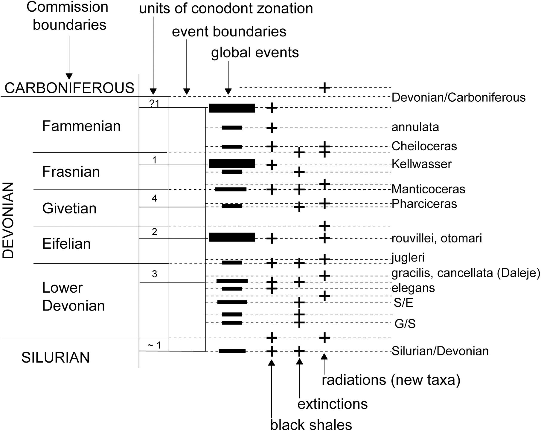
FIGURE 8. A diagram showing the relationship between Devonian natural events and the proposed chronostratigraphic boundaries of the Subcommission on Devonian Stratigraphy (redrawn after Walliser, 1985; Figure 1; used with the permission of the copyright holder, Courier Forschunginstitut Senckenberg).
For similar statements, we can turn to Newell (1966), quoted above, or Cloud (1972, pp. 537–538), who noted that “because time is continuous and without natural subdivisions, it becomes necessary in all historical science to identify events or broad modalities that set off one part of the sequence from preceding and following parts so as to bring out historical trends.” And, Bleeker (2004a, p. 219), who stressed that “boundaries should be placed at key events or transitions in the stratigraphic record, to highlight important milestones in the evolution of our planet.” These are the most informative boundaries, and they built a remarkable chronostratigraphy that worked well between about 1850 and 1950.
One of the primary goals of the ICS was to standardize the chronostratigraphic scale, and that was both laudable and still needs to be done. But, if I were to write a very short history of the chronostratigraphic work of the ICS, I would simply quote the old aphorism, that it was “the road to hell paved with good intentions.” We still need to standardize the chronostratigraphic scale. My hope is that the ICS and all interested in that goal will rethink the philosophy and practices by which this is being done, and abandon the inconsistencies and non-scientific concepts that have characterized GSSP-based chronostratigraphy for more than half a century. Then, we can move forward to produce the most informative chronostratigraphy possible based on a consistent methodology that allows updating (i.e., narrowing) boundary intervals corresponding to evolutionary turnovers (and other significant events) as new and additional data become available. In this way, chronostratigraphy can best reflect the present state of knowledge and is amenable to higher precision. Casting an arbitrary time point in “gold,” such as a GSSP, implicitly assumes that 100% of the data (i.e., of the relevant stratigraphic record) around this point are already known, which is not only presumptuous but represents a non-scientific stance, given the discontinuous nature of the record.
Author Contributions
The author confirms being the sole contributor of this work and approved it for publication.
Conflict of Interest Statement
The authors declare that the research was conducted in the absence of any commercial or financial relationships that could be construed as a potential conflict of interest.
Acknowledgments
I am grateful to many members of the ICS stratigraphic subcommissions and to many of my research collaborators, who have taught me much about chronostratigraphic principles and practice. The comments of the reviewers (Jean Guex and Francis Hirsch) and the associate editor (Hugo Bucher) improved the content and clarity of the manuscript.
References
Ager, D. V. (1984). “The stratigraphic code and what it implies,” in Catastrophes and Earth History: The New Uniformitarianism, eds W. A. Berggren and J. A. Van Couvering (Princeton, NJ: Princeton University Press), 91–100. doi: 10.1515/9781400853281.91
Albritton, C. C. Jr. (1986). The Abyss of Time: Changing Conceptions of the Earth’s Antiquity after the Sixteenth Century. Los Angeles, CA: Jeremy P. Tarcher, Inc.
Alpert, S. P. (1979). “Trace fossils and the basal Cambrian boundary,” in Trace Fossils 2, eds T. P. Crimes and J. C. Harper (Liverpool: Seel House Press),1–8.
Arduino, G. (ed.). (1760). “Letter by Arduino to Antonio Valisnieri, professor of natural history,” in Nuova Raccolta di Opuscoli Scientifici e Filologici del Padre Abate Angiolo Calogierà, Venice, Vol. 6 (Padua: University of Padua),142–143.
Aubry, M.-P., Berggren, W. A., Van Couvering, J. A., and Steininger, F. (1999). Problems in chronostratigraphy: stages, series, unit and boundary stratotypes, global stratotype section and point and tarnished golden spikes. Earth Sci. Rev. 46, 99–148. doi: 10.1016/s0012-8252(99)00008-2
Becker, R. T., Gradstein, F. M., and Hammer, O. (2012). “The Devonian Period,” in The Geologic Time Scale 2012, eds F. M. Gradstein, J. G. Ogg, M. D. Schmitz, and G. M. Ogg (Amsterdam: Elsevier), 559–601. doi: 10.1016/b978-0-444-59425-9.00022-6
Bell, W. C. (1959). Uniformitarianism or uniformity. Am. Assoc. Pet. Geol. Bull. 43, 2862–2865. doi: 10.1306/0bda5f69-16bd-11d7-8645000102c1865d
Berggren, W. A. (1998). “The Cenozoic Era: Lyellian (chrono)stratigraphy and nomenclatural reform at the millennium,” in Lyell: The Past is the Key to the Present, Vol. 143, eds D. J. Blundell and A. C. Scott (London: Geological Society), 111–132. doi: 10.1144/gsl.sp.1998.143.01.10
Berggren, W. A., and van Couvering, J. A. (1978). “Biochronology,” in Contributions to the Geological Time Scale, Vol. 6, eds G. V. Cohee, M. F. Glaessner, and H. D. Hedberg (Tulsa, OK: AAPG), 39–55.
Berry, W. B. N. (1987a). Growth of a Prehistoric Time Scale Based on Organic Evolution. Revised Edition. Palo Alto, CA: Blackwell.
Berry, W. B. N. (1987b). The Ordovician-Silurian boundary: new data, new concerns. Lethaia 20, 209–216. doi: 10.1111/j.1502-3931.1987.tb02039.x
Bleeker, W. (2004a). “Toward a “natural” Precambrian time scale,” in A Geologic Time Scale 2004, eds F. M. Gradstein, J. G. Ogg and A. G. Smith (Cambridge: Cambridge University Press), 141–146.
Bleeker, W. (2004b). Towards a “natural” time scale for the Precambrian—a proposal. Lethaia 37, 219–222. doi: 10.1080/00241160410006456
Bookstein, F. L., Gingerich, P. D., and Kluge, A. G. (1978). Hierarchical linear modeling of the tempo and mode of evolution. Paleobiology 4, 120–134. doi: 10.1017/S0094837300005807
Brasier, M., Cowie, J., and Taylor, M. (1994). Decision on the Precambrian-Cambrian boundary stratotype. Episodes 17, 3–8.
Brasier, M. D. (1989). “Towards a biostratigraphy of the earliest skeletal biotas,” in The Precambrian-Cambrian Boundary, Vol. 12, eds J. W. Cowie and M. D. Brasier (Oxford: Oxford University Press), 117–165.
Brosse, M., Bucher, H., Bagherpour, B., Baud, A., Frisk, A. M., Kuang, G., et al. (2015). Conodonts from the Early Triassic microbialite of Guangxi (South China): implications for the definition of the base of the Triassic System. Palaeontology 58, 563–584. doi: 10.1111/pala.12162
Brosse, M., Bucher, H., and Goudemand, N. (2016). Quantitative biochronology of the Permian-Triassic boundary in South China based on conodont unitary associations. Earth Sci. Rev. 155, 153–171. doi: 10.1016/j.earscirev.2016.02.003
Carter, R. M. (1974). A New Zealand case-study of the need for local time-scales. Lethaia 7, 181–202. doi: 10.1111/j.1502-3931.1974.tb00896.x
Chamberlin, T. C. (1909). Diastrophism as the ultimate basis of correlation. J. Geol. 17, 685–693. doi: 10.1086/621676
Chulpáč, I., and Vacek, F. (2003). Thirty years of the first international stratotype: the Silurian-Devonian boundary at Klonk and its present status. Episodes 26, 10–15.
Cloud, P. (1972). A working model of the primitive earth. Am. J. Sci. 272, 537–548. doi: 10.2475/ajs.272.6.537
Cloud, P. (1987). Trends, transitions, and events in Cryptozoic history and their calibration; apropos recommendations by the Subcommission on Precambrian Stratigraphy. Precambrian Res. 37, 257–265. doi: 10.1016/0301-9268(87)90070-2
Cohen, K. M., Harper, D. A. T., and Gibbard, P. L. (2018). International Chronostratigraphic Chart 2018/08. International Commission on Stratigraphy. Paris: IUGS.
Cooper, R. A., Sadler, P. M., Hammer, O., and Gradstein, F. M. (2012). “The Ordovician Period,” in The Geologic Time Scale 2012, eds F. M. Gradstein, J. G. Ogg, M. D. Schmitz, and G. M. Ogg (Amsterdam: Elsevier), 489–523. doi: 10.1016/b978-0-444-59425-9.00020-2
Cope, J. C. W. (1996). The role of the secondary standard in stratigraphy. Geol. Mag. 133, 107–110. doi: 10.1017/s0016756800007299
Cowie, J. W. (1981). The Proterozoic-Phanerozoic transition and the Precambrian-Cambrian boundary. Precambrian Res. 15, 199–206. doi: 10.1016/0301-9268(81)90051-6
Cowie, J. W., Ziegler, W., Boucot, A. J., Bassett, M. G., and Remane, J. (1986). Guidelines and statutes of the International Commission on Stratigraphy (ICS). Cour. Forschungsinstitut Senckenb. 83, 1–14.
Crimes, T. P. (1989). “Trace fossils,” in The Precambrian-Cambrian Boundary, Vol. 12, eds J. W. Cowie and M. D. Brasier (Oxford: Oxford University Press), 166–185.
Crook, K. A. W. (1989). Why the Precambrian timescale should be chronostratigraphic: a response to recommendations by the Subcommission of Precambrian Stratigraphy. Precambrian Res. 43, 143–150. doi: 10.1016/0301-9268(89)90009-0
Davydov, V. I., Korn, D., Schmitz, M. D., Gradstein, F. M., and Hammer, O. (2012). “The Carboniferous Period,” in The Geologic Time Scale 2012, eds F. M. Gradstein, J. G. Ogg, M. D. Schmitz, and G. M. Ogg (Amsterdam: Elsevier), 603–651. doi: 10.1016/b978-0-444-59425-9.00023-8
Dawkins, R. (1996). The Blind Watchmaker: Why the Evidence of Evolution Reveals a Universe Without Design. New York, NY: W. W. Norton & Co.
Dunbar, C. O., and Rodgers, J. (1958). Principles of Stratigraphy. New York, NY: John Wiley and Sons, Inc.
Fang, F. C., and Casadevall, A. (2011). Editorial: reductionistic and holistic science. Infect. Immmun. 79, 1401–1404. doi: 10.1128/iai.01343-10
Finney, S. C., and Edwards, L. E. (2016). The “Anthropocene” epoch: scientific decision or political statement? GSA Today 26, 4–10. doi: 10.1130/gsatg270a.1
Folk, R. L., and Ferm, J. C. (1966). A portrait of Paul D. Krynine. J. Sediment. Petrol. 36, 853–863. doi: 10.2110/jsr.36.351
Fortey, R. A. (1973). Charles Lapworth and the biostratigraphic paradigm. J. Geol. Soc. Lond. 150, 209–218. doi: 10.1144/gsjgs.150.2.0209
Gehling, J. G., Jensen, S., Droser, M. L., Myrow, P. M., and Narbonne, G. M. (2001). Burrowing below the basal Cambrian GSSP, Fortune Head, Newfoundland. Geol. Mag. 138, 213–218. doi: 10.1017/s001675680100509x
Gibbard, P. L., Head, M. J., Walker, M. J. C., and The Subcommission on Quaternary Stratigraphy (2010). Formal ratification of the Quaternary System/Period and the Pleistocene Series/Epoch with a base at 2.58 Ma. J. Quat. Sci. 25, 96–102. doi: 10.1002/jqs.1338
Gignoux, M. (1955). Stratigraphic Geology [English Translation of 1950], 4th Edn. San Francisco, CA: W. H. Freeman & Co.
Gilluly, J. (1949). Distribution of mountain building in geologic time. Bull. Geol. Soc. Am. 60, 561–590. doi: 10.1130/0016-7606(1949)60[561:DOMBIG]2.0.CO;2
Giordano, N., Rigo, M., Ciarapica, G., and Bertinelli, A. (2010). New biostratigraphical constraints for the Norian/Rhaetian boundary: data from Lagonegro basin, Southern Apennines, Italy. Lethaia 43, 573–586. doi: 10.1111/j.1502-3931.2010.00219.x
Gladenkov, Y. (2014). Some debatable problems of stratigraphic classification. Geophys. Res. Abstr. 16, EGU2014–EGU3615.
Goudemand, N., Orchard, M. J., Bucher, H., and Jenks, J. (2012). The elusive origin of Chiosella timorensis (conodont Triassic). Geobios 45, 199–207. doi: 10.1016/j.geobios.2011.06.001
Gradstein, F. M. (2012). “Biochronology,” in The Geologic Time Scale 2012, eds F. M. Gradstein, J. G. Ogg, M. D. Schmitz, and G. M. Ogg (Amsterdam: Elsevier), 43–61. doi: 10.1016/b978-0-444-59425-9.00003-2
Gradstein, F. M., Finney, S. C., Lane, R., and Ogg, J. G. (2003). ICS on stage. Lethaia 36, 371–378. doi: 10.1080/00241160310006411
Gradstein, F. M., Ogg, J. G., Schmitz, M. D., and Ogg, G. M., eds (2012). The Geologic Time Scale 2012. Amsterdam: Elsevier.
Gradstein, F. M., Ogg, J. G., and Smith, A. G., eds (2004a). A Geologic Time Scale 2004. Cambridge: Cambridge University Press. doi: 10.4095/215638
Gradstein, F. M., Ogg, J. G., and Smith, A. G. (2004b). “Chronostratigraphy: linking time and rock,” in A Geologic Time Scale 2004, eds F. M. Gradstein, J. G. Ogg and A. G. Smith (Cambridge: Cambridge University Press), 20–46. doi: 10.4095/215638
Gradstein, F. M., Ogg, J. G., Smith, A. G., Bleeker, W., and Lourens, L. J. (2004c). A new geologic time scale with special reference to Precambrian and Neogene. Episodes 27, 83–100.
Guex, J., Galster, F., and Hammer, O. (2016). Discrete Biochronological Time Scales. Heidelberg: Springer. doi: 10.1007/978-3-319-21326-2
Harland, W. B. (1992). Stratigraphic regulation and guidance: a critique of current tendencies in stratigraphic codes and guides. Geol. Soc. Am. Bull. 104, 1231–1235. doi: 10.1130/0016-7606(1992)104<1231:SRAGAC>2.3.CO;2
Harland, W. B., Armstrong, R. L., Cox, A. V., Craig, L. E., Smith, A. G., and Smith, D. G. (1990). A Geologic Time Scale. Cambridge: Cambridge University Press.
Harland, W. B., Cox, A. V., Llewellyn, P. G., Pickton, C. A. G., Smith, A. G., and Walters, R. (1982). A Geologic Time Scale. Cambridge: Cambridge University Press.
Hayami, I., and Ozawa, T. (1975). Evolutionary models of lineage-zones. Lethaia 8, 1–14. doi: 10.1111/j.1502-3931.1975.tb00908.x
Head, M. J., Aubry,M-P., Walker, M., Miller, K. G., and Pratt, B. R. (2017). A case for formalizing subseries (subepochs) of the Cenozoic Era. Episodes 40, 2–7. doi: 10.18814/epiiugs/2017/v40i1/017004
Heckel, P. H., and Clayton, G. (2006). The Carboniferous System. Use of the new official names for the subsystems, series, and stages. Geol. Acta 4, 403–407.
Hedberg, H. D. (1948). Time-stratigraphic classification of sedimentary rocks. Bull. Geol. Soc. Am. 59, 447–462. doi: 10.1130/0016-7606(1948)59[447:TCOSR]2.0.CO;2
Hedberg, H. D. (1951). Nature of time-stratigraphic units and geologic time units. AAPG Bull. 35, 1077–1081. doi: 10.1306/3d934223-16b1-11d7-8645000102c1865d
Hedberg, H. D. (1958). Stratigraphic classification and terminology. AAPG Bull. 42, 1881–1896. doi: 10.1306/0bda5b85-16bd-11d7-8645000102c1865d
Hedberg, H. D. (1965a). Chronostratigraphy and biostratigraphy. Geol. Mag. 102, 451–461. doi: 10.1017/s0016756800053723
Hedberg, H. D. (1965b). Earth history and the record in the rocks. Proc. Am. Philos. Soc. 109, 99–104.
Hedberg, H. D. (1968). Some views on chronostratigraphic classification. Geol. Mag. 105, 192–199. doi: 10.1017/s0016756800052614
Hedberg, H. D. (ed.). (1976). International Stratigraphic Guide: A Guide to Classification, Terminology, and Procedure. New York, NY: John Wiley and Sons.
Hilgen, F. J., Lourens, L. J., Van Dam, J. A., Beu, A. G., Boyes, A. F., Cooper, R. A., et al. (2012). “The Neogene Period,” in The Geologic Time Scale 2012, eds F. M. Gradstein, J. G. Ogg, M. D. Schmitz, and G. M. Ogg (Amsterdam: Elsevier), 923–978. doi: 10.1016/b978-0-444-59425-9.00029-9
Holland, C. H., Bassett, M. G., and Rickards, R. B. (2003). Stability in stratigraphy. Lethaia 36, 69–70. doi: 10.1080/00241160310001209
Jiang, H., Aldridge, R. J., Lai, X., Yan, C., and Sun, Y. (2011). Phylogeny of the conodont genera Hindeodus and Isarcicella across the Permian-Triassic boundary. Lethaia 44, 374–382. doi: 10.1111/j.1502-3931.2010.00248.x
Kaiser, S. I. (2009). The Devonian/Carboniferous boundary stratotype section (La Serre, France) revisited. Newsl. Stratigr. 43, 195–205. doi: 10.1127/0078-0421/2009/0043-0195
Kaiser, S. I., and Corradini, C. (2008). Should the Devonian/Carboniferous boundary be redefined? SDS Newsl. 23, 55–56.
Kennedy, W. J., Gale, A. S., Huber, B. T., Petrizzo, M. R., Bown, P., and Jenkyns, H. C. (2017). The global boundary stratotype section and point (GSSP) for the base of the Albian Stage of the Cretaceous, the Col de Pre-Guittard section, Amazon, Dvôme, France. Episodes 40, 177–188. doi: 10.18814/epiiugs/2017/v40i3/017021
Kitts, D. B. (1989). Geological time and psychological time. Earth Sci. Hist. 8, 190–191. doi: 10.17704/eshi.8.2.4102132n21644667
Krassilov, V. (1978). Organic evolution and natural stratigraphical classification. Lethaia 11, 93–104. doi: 10.1111/j.1502-3931.1978.tb01292.x
Krystyn, L. (2010). Decision report on the defining event for the base of the Rhaetian stage. Albertiana 38, 11–12.
Krystyn, L., Boquerel, H., Kuerschner, W., Richoz, S., and Gallet, Y. (2007). Proposal for a candidate GSSP for the base of the Rhaetian Stage. N. M. Mus. Nat. Hist. Sci. Bull. 41, 189–199.
Lamolda, M. A., Paul, C. R. C., Peryt, D., and Pons, J. M. (2014). The global boundary stratotype and section point (GSSP) for the base of the Santonian Stage, “Cantera de Margas”, Olazagutia, northern Spain. Episodes 37, 2–13.
Lespérance, P. J., Barnes, C. R., Berry, W. B. M., Boucot, A. J., and Mu, E. (1987). The Ordovician-Silurian boundary stratotype: consequences of its approval by the IUGS. Lethaia 20, 217–222. doi: 10.1111/j.1502-3931.1987.tb02040.x
Lucas, S. G. (2010). The Triassic chronostratigraphic scale: history and status. Geol. Soc. Lond. Spec. Publ. 334, 17–39. doi: 10.1144/sp334.2
Lucas, S. G. (2016). Base of the Rhaetian and a critique of conodont-based chronostratigraphy. Albertiana 43, 24–32.
Lucas, S. G., and Shen, S. (2018). “The Permian chronostratigraphic scale: history, status and prospectus,” in The Permian Timescale, Vol. 450, eds S. G. Lucas, and S. Z. Shen (London: Geological Society). doi: 10.1144/SP450.3
Lyell, C. (1855). A Manual of Elementary Geology, 5th Edn. London: John Murray. doi: 10.5962/bhl.title.50205
Marcou, J. (1862). Observations on the terms “Pénéen,” “Permian,” and “Dyas.” Proc. Boston Soc. Nat. Hist. 9, 33–36. doi: 10.1017/s135946560000215x
McLaren, D. J. (1977). “The Silurian Devonian boundary committee: a final report,” in The Silurian-Devonian Boundary, ed. A. Martinsson (Stuttgart: IUGS), 1–34.
Mei, S., and Henderson, C. M. (2001). Evolution of Permian conodont provincialism and its significance in global correlation and paleoclimate implication. Palaeogeogr. Palaeoclimatol. Palaeoecol. 170, 237–260. doi: 10.1016/s0031-0182(01)00258-9
Melchin, M. J., Rong, J., Gradstein, F., Kopen, T. N., and Finney, S. C. (2004). Stability in stratigraphy. Lethaia 37, 124–125. doi: 10.1080/00241160410005025
Melchin, M. J., Sadler, P. M., Cramer, B. D., Cooper, R. A., Gradstein, F. M., and Hammer, O. (2012). “The Silurian Period,” in The Geologic Time Scale 2012, eds F. M. Gradstein, J. G. Ogg, M. D. Schmitz, and G. M. Ogg (Amsterdam: Elsevier), 525–558. doi: 10.1016/b978-0-444-59425-9.00021-4
Meyen, S. V. (1976). The concepts of “naturalness” and “synchroneity” in stratigraphy. Int. Geol. Rev. 18, 80–88. doi: 10.1080/00206817609471173
Monnet, C., Brayard, A., and Bucher, H. (2015). “Ammonoids and quantitative biochronology—a unitary association perspective,” in Ammonoid Paleobiology: From Macroevolution to Paleogeography, Vol. 44, eds C. Klug, D. Korn, K. De Baets, I. Kruta, and R. H. Mapes (Dordrecht: Springer), 277–298. doi: 10.1007/978-94-017-9633-0_11
Monnet, C., and Bucher, H. (2002). Cenomanian (early Late Cretaceous) ammonoid faunas of Western Europe. Part 1: biochronology (unitary associations) and diachronism of datums. Eclog. Geol. Helv. 95, 57–93.
Moore, R. C. (1940). Carboniferous-Permian boundary. Am. Assoc. Pet. Geol. Bull. 24, 282–336. doi: 10.1306/3d9331a6-16b1-11d7-8645000102c1865d
Murchison, R. I. (1839). The Silurian System, Founded on Geological Researches in the Counties of Salop, Hereford, Radnor, Montgomery, Caermarthen, Brecon, Pembroke, Monmouth, Gloucester, Worcester, and Stafford: With Descriptions of the Coalfields and Overlying Formations, Part 1. London: John Murray.
Murchison, R. I. (1841). First sketch of some of the principal results of a second geological survey of Russia. Philos. Mag. 19, 417–422. doi: 10.1080/14786444108650460
Murchison, R. I. (1862). On the inapplicability of the new term ‘Dyas’ to the ‘Permian’ group of rocks, as proposed by Dr. Geinitz. Geologist 5, 4–10. doi: 10.1017/s1359465600003464
Murphy, M. A. (1994). Fossils as a basis for chronostratigraphic interpretation. Neues Jahrb. Geol. Paläontol. Abh. 192, 255–271.
Ogg, J. G., Hinnov, L. A., and Huang, C. (2012a). “Cretaceous,” in The Geologic Time Scale 2012, eds F. M. Gradstein, J. G. Ogg, M. D. Schmitz, and G. M. Ogg (Amsterdam: Elsevier), 793–853. doi: 10.1016/b978-0-444-59425-9.00027-5
Ogg, J. G., Hinnov, L. A., and Huang, C. (2012b). “Jurassic,” in The Geologic Time Scale 2012, eds F. M. Gradstein, J. G. Ogg, M. D. Schmitz, and G. M. Ogg (Amsterdam: Elsevier), 731–791. doi: 10.1016/b978-0-444-59425-9.00026-3
Orchard, M. J., Grãdinaru, E., and Nicora, A. (2007). A summary of the conodont succession around the Olenekian-Anisian boundary at Deşli Caira, North Dobrogea, Romania. N. M. Mus. Nat. Hist. Sci. Bull. 41, 341–346.
Palotai, M., Pálfy, J., and Sasvári, Á. (2017). Structural complexity at and around the Triassic-Jurassic GSSP at Kuhjoch, Northern Calcareous Alps, Austria. Int. J. Earth Sci. 106, 2475–2487. doi: 10.1007/s00531-017-1450-4
Pearson, P. N., MacMillan, I. K., Wade, B. S., Jones, T. D., Coxall, H. K., Bown, P. R., et al. (2008). Extinction and environmental change across the Eocene-Oligocene boundary in Tanzania. Geology 36, 179–182. doi: 10.1130/G24308A.1
Peng, S., and Babcock, L. E. (2011). Continuing progress on chronostratigraphic subdivision of the Cambrian System. Bull. Geosci. 86, 391–396. doi: 10.1130/g24308a.1
Peng, S., Babcock, L. E., and Cooper, R. A. (2012). “The Cambrian Period,” in The Geologic Time Scale 2012, eds F. M. Gradstein, J. G. Ogg, M. D. Schmitz, and G. M. Ogg (Amsterdam: Elsevier), 437–488. doi: 10.1016/b978-0-444-59425-9.05001-0
Phillips, J. (1860). Life on Earth: Origin and Succession. Cambridge: MacMillan and Co. doi: 10.5962/bhl.title.22153
Pillans, B., and Gibbard, P. (2012). “The Quaternary Period,” in The Geologic Time Scale 2012, eds F. M. Gradstein, J. G. Ogg, M. D. Schmitz, and G. M. Ogg (Amsterdam: Elsevier), 979–1010. doi: 10.1016/b978-0-444-59425-9.00030-5
Remane, J. (1991). The Jurassic-Cretaceous boundary: problems of definition and procedure. Cretac. Res. 12, 447–453. doi: 10.1016/0195-6671(91)90001-S
Remane, J. (2003). Chronostratigraphic correlations: their importance for the definition of geochronologic units. Palaeogeogr. Palaeoclimatol. Palaeoecol. 196, 7–18. doi: 10.1016/s0031-0182(03)00310-9
Remane, J., Bassett, M. G., Cowie, J. C., Gohrbandt, K. H., Lane, H. R., Michelsen, O., and Wang, N., with the Cooperation of Members of ICS (1996). Revised guidelines for the establishment of global chronostratigraphic standards by the International Commission on Stratigraphy (ICS). Episodes 19, 77–81.
Richter, R. (1956). Chronologische Grenzen und die Grenze zwischen Unter-Devon und Mittel-Devon. Senckenb. Lethaea 37, 337–342.
Robb, L. J., Knoll, A. H., Plumb, K. A., Shields, G. A., Strauss, H., and Veizer, J. (2004). “The Precambrian: Archean and Proterozoic eons,” in A Geologic Time Scale 2004, eds F. M. Gradstein, J. G. Ogg and A. G. Smith (Cambridge: Cambridge University Press), 129–140. doi: 10.1017/cbo9780511536045.010
Rong, J., Melchin, M., Williams, S. H., Koren, T. N., and Vernices, J. (2008). Report of the restudy of the defined global stratotype of the base of the Silurian. Episodes 31, 315–318.
Rudwick, M. (1996). Cuvier and Brongniart, William Smith, and the reconstruction of geohistory. Earth Sci. Hist. 15, 25–36. doi: 10.17704/eshi.15.1.h25k254u61374h00
Sadler, P. M., Cooper, R. A., and Melchin, M. (2009). High-resolution, early Paleozoic (Ordovician-Silurian) time scales. Geol. Soc. Am. Bull. 121, 887–906. doi: 10.1130/b26357.1
Salvador, A. (1994). International Stratigraphic Guide: A Guide to Classification, Terminology, and Procedure. New York, NY: John Wiley and Sons. doi: 10.1130/9780813774022
Smith, A. G., Barry, T., Bown, P., Cope, J., Gale, A., Gibbard, P., et al. (2014). “GSSPs, global stratigraphy and correlation,” in Strata and Time: Probing the Gaps in our Understanding, Vol. 404, eds D. G. Smith, R. J. Bailey, P. M. Burgess and A. J. Fraser (London: Geological Society), 37–67. doi: 10.1144/sp404.8
Teichert, C. (1958). Some biostratigraphical concepts. Bull. Geol. Soc. Am. 69, 99–120. doi: 10.1130/0016-7606(1958)69[99:SBC]2.0.CO;2
Vai, G. B. (2001). GSSP, IUGS and IGC: an endless story toward a common language in Earth sciences. Episodes 24, 29–31.
Van Kranendonk, M. J., Altermannm, W., Beard, B. L., Hoffman, P. F., Johnson, C. M., Kasting, J. F., et al. (2012). “A chronostratigraphic division of the Precambrian,” in The Geologic Time Scale 2012, eds F. M. Gradstein, J. G. Ogg, M. D. Schmitz, and G. M. Ogg (Amsterdam: Elsevier), 299–392. doi: 10.1016/b978-0-444-59425-9.00016-0
Vandenberghe, N., Hilgen, F. J., Speijer, R. P., Ogg, J. G., Gradstein, F. M., Hammer, O., et al. (2012). “The Paleogene Period,” in The Geologic Time Scale 2012, eds F. M. Gradstein, J. G. Ogg, M. D. Schmitz, and G. M. Ogg (Amsterdam: Elsevier), 855–921.
von Hillebrandt, A., Kürschner, W. M., and Krystyn, L. (2007). A candidate GSSP for the base of the Jurassic in the Northern Calcareous Alps (Kuhjoch section, Karwendel Mountains, Tyrol, Austria). Int. Subcommiss. Jurassic Stratigr. Newsl. 34, 2–20.
von Hillebrandt, A., Krystyn, L., Kürschner, W. M., Bonis, N. R., Ruhl, M., Richoz, S., Schobben, M. A.N., et al. (2013). The global stratotype sections and point (GSSP) for the base of the Jurassic System at Kuhjoch (Karwendel Mountains, Northern Calcareous Alps, Tyrol, Austria). Episodes 36, 162–198.
Voosen, P. (2018). New geological age comes under fire. Science 361, 537–538. doi: 10.1126/science.361.6402.537
Walliser, O. H. (1984). Pleading for a natural D/C boundary. Cour. Forschungsinstitut Senckenb. 67, 241–246.
Walliser, O. H. (1985). Natural boundaries and the Commission boundaries in the Devonian. Cour. Forschungsinstitut Senckenb. 75, 401–408.
Walliser, O. H. (1986). “Towards a more critical approach to bio-events,” in Global Bio-Events, Vol. 8, ed. O. H. Walliser (Berlin: Springer), 5–16. doi: 10.1007/bfb0010187
Walliser, O. H. (1996). Patterns and causes of global events,” in Global Events and Event Stratigraphy in the Phanerozoic, ed. O. H. Walliser (Berlin: Springer), 7–19. doi: 10.1007/978-3-642-79634-0_2
Walsh, S. L. (1998). Fossil datum and paleobiological event terms, paleontostratigraphy, chronostratigraphy, and the definitions of land mammal “age” boundaries. J. Vertebr. Paleontol. 18, 150–179. doi: 10.1080/02724634.1998.10011041
Walsh, S. L., Gradstein, F. M., and Ogg, J. G. (2004). History, philosophy, and application of the Global Stratotype Section and Point (GSSP). Lethaia 37, 201–218. doi: 10.1080/00241160410006500
Waters, C. N., Zalasiewicz, J. A., Williams, M., Ellis, M. A., and Snelling, A. M., eds (2014). A Stratigraphical Basis for the Anthropocene, Vol. 395. London: Geological Society. doi: 10.1144/sp395.18
Weddige, K., and Ziegler, W. (1979). Evolutionary patterns in Middle Devonian conodont genera Polygnathus and Icriodus. Geol. Palaeontol. 13, 157–164.
Wheeler, H. E., and Beesley, E. M. (1948). Critique of the time-stratigraphic concept. Bull. Geol. Soc. Am. 59, 75–86. doi: 10.1130/0016-7606(1948)59[75:COTTC]2.0.CO;2
Williams, H. S. (1901). The discrimination of time values in geology. J. Geol. 9, 570–585. doi: 10.1086/620952
Wilmarth, M. G. (1925). The geologic time classification of the United States Geological Survey compared with other classifications accompanied by the original definitions of era, period and epoch terms. U.S. Geol. Surv. Bull. 769:138.
Witzke, B. J. (2013). Correlating Ordovician cratonic sequences: shoreward sediment condensation and transgressive sand facies in the Ancell, Platteville, and Galena groups, Midcontinent North America. Geol. Soc. Am. Abstr. Prog. 45:891.
Zakharov, Y. (2010). New information on biostratigraphy of the Mud section. Spiti Albertiana 38, 4–7.
Zhamoida, A. I. (1984). Comparing the Soviet stratigraphic code with the international guide. Episodes 7, 9–11.
Zhou, Z. (2017). Permian basinal ammonoid sequence in Nanpanjiang area of South China—possible overlap between basinal Guadalupian and platform-based Lopingian. J. Paleontol. Mem. 74, 1–95. doi: 10.1017/jpa.2016.128
Keywords: chronostratigraphy, boundary stratotype, International Commission on Stratigraphy (ICS), Global Stratotype Section and Point (GSSP), arbitrary decisions, reductionism
Citation: Lucas SG (2018) The GSSP Method of Chronostratigraphy: A Critical Review. Front. Earth Sci. 6:191. doi: 10.3389/feart.2018.00191
Received: 06 July 2018; Accepted: 17 October 2018;
Published: 06 November 2018.
Edited by:
Hugo F. R. Bucher, Universität Zürich, SwitzerlandReviewed by:
Francis Hirsch, Geological Survey of Israel, IsraelJean Rene Guex, University of Lausanne (UNIL), Switzerland
Copyright © 2018 Lucas. This is an open-access article distributed under the terms of the Creative Commons Attribution License (CC BY). The use, distribution or reproduction in other forums is permitted, provided the original author(s) and the copyright owner(s) are credited and that the original publication in this journal is cited, in accordance with accepted academic practice. No use, distribution or reproduction is permitted which does not comply with these terms.
*Correspondence: Spencer G. Lucas, spencer.lucas@state.nm.us