Carbon Dynamics During the Formation of Sea Ice at Different Growth Rates

Introduction

While the polar regions are generally considered an important sink for atmospheric carbon dioxide (CO₂), the influence of sea ice on air-sea carbon dynamics is unclear. Originally assumed to be an impermeable lid hindering air-sea gas exchange (e.g., Stephens and Keeling, 2000; Tison et al., 2002), sea ice has since been recognized to play an active role in the marine carbon cycle, as both biological and physico-chemical processes take place within and around the ice (Vancoppenolle et al., 2013). The sea-ice zone is believed to act as a sink for atmospheric CO₂ on an annual basis (Rysgaard et al., 2011), although the direction and magnitude of the carbon flux differ between the different stages of the seasonal sea-ice growth and decay cycle and also appear to depend on the methods used (Miller et al., 2015).

During the period of ice formation, the conceptual model developed by Rysgaard et al. (2011) predicts CO₂ release to the atmosphere. When ice is formed, the majority of ions and gases present in the original sea water are expelled from the crystal lattice, whereby liquid brine intrusions with high salinities and gas concentrations are formed between ice crystals (Petrich and Eicken, 2016). A small part of the brine supersaturated in CO₂ is then predicted to be expelled to the sea-ice surface and to release CO₂ to the atmosphere (Rysgaard et al., 2011). Small, positive CO₂ fluxes out of young, newly formed sea ice have indeed been detected in the field (Else et al., 2011; Geilfus et al., 2013; Barber et al., 2014; Nomura et al., 2018) and in artificial sea ice (Nomura et al., 2006; Geilfus et al., 2016; Kotovitch et al., 2016). However, while the CO₂ flux out of the young ice itself is likely positive (upward), the overall CO₂ flux during ice formation in the marginal sea ice zone may be negative, depending on the presence of open water, including leads and polynyas, which may enhance CO₂ uptake from the air (e.g., Anderson et al., 2004; Loose et al., 2011).

Sea-ice formation also has the potential to export carbon to deeper water layers (Rysgaard et al., 2007, 2011). Carbon dioxide-enriched brine produced during sea-ice formation could sink to levels below the surface mixed layer and lead to a net annual uptake of atmospheric CO₂ of up to 33 Tg C yr⁻¹, according to Rysgaard et al. (2011). This uptake could be further enhanced by the precipitation of calcium carbonate (CaCO₃) minerals, namely ikaite. During the formation of ikaite, CO₂ is produced, and the ratio of total alkalinity (A_T) to dissolved inorganic carbon (DIC) of the brine is reduced (DIC refers here to the dissolved fraction of TIC; we use TIC for the remainder of this manuscript since our samples were unfiltered and may have contained solid carbonates). Assuming that the CO₂ enriched brine sinks to deeper water levels while the ikaite crystals stay in the ice, this would lead to an enrichment of surface water alkalinity during ice melt (Rysgaard et al., 2007). This, in turn, could result in a higher uptake of atmospheric CO₂, on the order of 83 Tg C yr⁻¹, globally (Rysgaard et al., 2011). This effect might be more pronounced at lower ice temperatures, since ikaite precipitation is more likely (in an open system) at the higher brine salinities encountered at lower temperatures (Papadimitriou et al., 2013). Differences in ice temperatures have thus been suggested to explain different A_T to TIC ratios observed at multiple field locations (Rysgaard et al., 2007, 2009). However, the importance of ikaite precipitation for atmospheric CO₂ uptake is debatable, as is transport below the mixed layer. The latter almost certainly does not occur in all sea-ice environments (Loose et al., 2011), and according to a recent modeling study (Moreau et al., 2016), the fraction of DIC exported to depth could be no more than 2% (about 4 Tg C yr⁻¹) of all DIC rejected during sea ice growth. This fraction was found to be even lower for a global warming scenario in a similar study conducted by Grimm et al. (2016) due to changes to the oceanic overturning circulation. However, Parmentier et al. (2013) also stressed the importance of open water in the sea-ice cover (i.e., leads and polynyas) for the formation of dense water needed for export to depth, which may not have been adequately represented in their model. Thus, as such open water areas may be more prevalent in a warming future (Parmentier et al., 2013), the export of carbon may also be enhanced.

The influence of the ice growth rate on TIC export from the forming ice has received little attention so far, but some insight might be gained from desalination studies, given that inorganic carbon is mostly present in dissolved form in seawater. Our understanding of sea-ice brine drainage processes is rapidly evolving, and mushy layer theory has been suggested as a useful model to explain the underlying mechanisms of sea-ice desalination (Feltham et al., 2006; Notz and Worster, 2009). This theory predicts gravity drainage to be the dominant desalination process during ice growth (Notz and Worster, 2009). Gravity drainage results from the temperature gradient across the ice, as high salinity brine formed at the lower temperatures in the upper layers of the ice overlies less saline, and thus less dense brine formed at the warmer temperatures closer to the sea ice-water interface. This unstable brine density profile eventually leads to convective overturning within the ice, when the density gradient and the ice thickness are large enough to provide the required potential energy to overcome the energy loss due to dissipation during convection (Wettlaufer et al., 1997). Thus, mushy layer theory predicts a delayed onset of desalination, which has been observed in laboratory ice growth studies (Wettlaufer et al., 1997; Notz and Worster, 2009).

The impact of different ice growth rates on gravity drainage is not straightforward. While the dependence of gravity drainage on the temperature gradient would suggest more effective desalination at colder ambient temperatures, desalination is hindered by lower ice permeability at these colder temperatures, which can limit the convection to the ice layers close to the ice-water interface (Notz and Worster, 2009). Both laboratory and numerical studies found that for constant boundary conditions (i.e., constant cooling), an inverse relationship between salt flux and growth rates holds, i.e., increased bulk ice salinity at faster growth rates as a result of the decreased permeability (Cox and Weeks, 1975; Wettlaufer et al., 1997; Griewank and Notz, 2013). Similarly, results from field studies comparing salinity profiles of ice cores to their growth rate history suggest that faster ice growth leads to higher retention of salt in sea ice (Nakawo and Sinha, 1981; Eicken, 1992; Gough et al., 2012). Assuming the TIC redistribution during ice formation is dominated by brine drainage, a higher retention of TIC in ice at faster ice growth rates is thus predicted.

The correlation between TIC and salinity could be disturbed by multiple abiotic and biological processes. Apart from biological transformations of TIC into organic substances, the precipitation of ikaite or the nucleation of CO₂ bubbles both lead to inorganic forms of carbon that could migrate within ice differently from dissolved salts (Vancoppenolle et al., 2013). Furthermore, both processes are dependent on the in-situ temperature and salinity conditions and are possibly interconnected: increased CO₂ partial pressure (pCO₂) at high salinities could lead to the formation of gas bubbles, which in turn could promote the precipitation of ikaite by lowering the CO₂ concentration in the brine (Papadimitriou et al., 2014). Therefore, TIC and salinity decoupling could be more pronounced in colder, and thus more saline, brine. Nevertheless, experimental and model studies on newly forming sea ice have found that ikaite precipitation and CO₂ outgassing to the atmosphere are small compared to the efflux of dissolved inorganic carbon with brine to the underlying water (Rysgaard et al., 2007; Sejr et al., 2011; Moreau et al., 2015; Kotovitch et al., 2016). This indicates that the transport in dissolved form is predominant, and the TIC signal should largely follow salinity. However, past laboratory experiments have been conducted at a single, relatively high temperature, and might not be representative of faster ice growth conditions.

In the context of the large uncertainties in the air-ice and ice-water carbon fluxes, transformation and transport processes within the ice, and the impact of different ice growth rates, further insight into carbon dynamics during sea-ice formation is needed. Therefore, we conducted laboratory experiments simulating ice formation at three different growth rates with discrete and continuous measurements of CO₂ system parameters in ice and water. In addition, we estimated the air-ice CO₂ flux using a carbon budget approach. In addition to discrete sample analyses, the installation of sensors in the ice and water, including thermistors, Dopbeam sonars, and a water salinity probe, allowed us to further investigate brine drainage processes.

Materials and Methods

Ice Growth Experiments

The ice growth experiments were conducted in a walk-in freezer at the Institute of Ocean Sciences in Sidney, BC, which is equipped with three separate refrigeration condensers. The condensers can be set to keep the ambient temperature of the freezer stable anywhere between 0°C and −45°C, apart from regular defrost intervals, when the temperature can increase by up to 10°C over a period of 1 h (in the case of the coldest experiments). Three ambient temperatures (−15°C, −25°C, and −40°C) were chosen to cover a wide range of ice growth rates within a temperature range observable in nature, and to be sufficiently cold to reach the desired thickness. The ambient conditions in the cold lab were monitored by a weather station (König, 2017), mean air temperatures and their standard deviations are listed in Table S2.

The cold lab contained a water tank (ca. 105 × 95 × 99 cm; Figure 1A) holding natural, open ocean seawater, which was collected on June 16, 2016, at Ocean Station P20 in the Northeast Pacific (50°N, 145°W) at a depth of 5 m. To minimize biological activity, the experiments were run in the dark and the water was filtered through a 1 μm filter and sterilized with a UV lamp for 24 h before the start of the experiment and whenever new seawater was added to the tank. Whereas in general, the seawater was re-used for the different experimental runs and additional seawater was only added on two occasions, tap water was added to the tank after each experiment, to counteract the increase in salinity due to evaporation and the removal of ice cores. This had a minor impact on the chemical composition of the seawater, observable as a slight increase in TIC relative to A_T. The tank was insulated on the sides, to prevent ice growth on the walls, and open at the top. To enable water sampling from underneath the ice, a sampling system with adjustable heating was installed in the tank, connecting multiple Tygon^® tubes from within the tank to a port outside the freezer (Figure 1A).

FIGURE 1

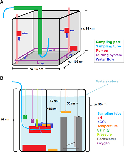
Figure 1. Schematic illustration of the experimental tank with its stirring and sampling systems (A) and all sensors discussed in this manuscript (B).

The first set of experiments was conducted with stirring to prevent stratification and ensure that all deployed sensors would measure seawater representative of the whole body of water. For a second set of experiments, the water was not stirred (except during water sampling to avoid sampling stratified layers) to allow brine plume detection, as well as to test the impact of mixing on the results of the previous runs. Each experiment was stopped (i.e., water and ice were sampled) once the ice thickness had reached about 20 cm. The stirring system was made up of a pump connected to PVC pipes arranged in a rectangle at the bottom (Figure 1A), which generated an observable vortex through the entire depth of the tank. In addition, two pumps were installed vertically at a depth of ca. 30 cm in order to prevent stratification.

An overview of all successful experimental runs is shown in Table 1, including ambient temperatures and whether or not the tank was stirred. A more comprehensive overview, including all (attempted) runs is given by König (2017).

TABLE 1

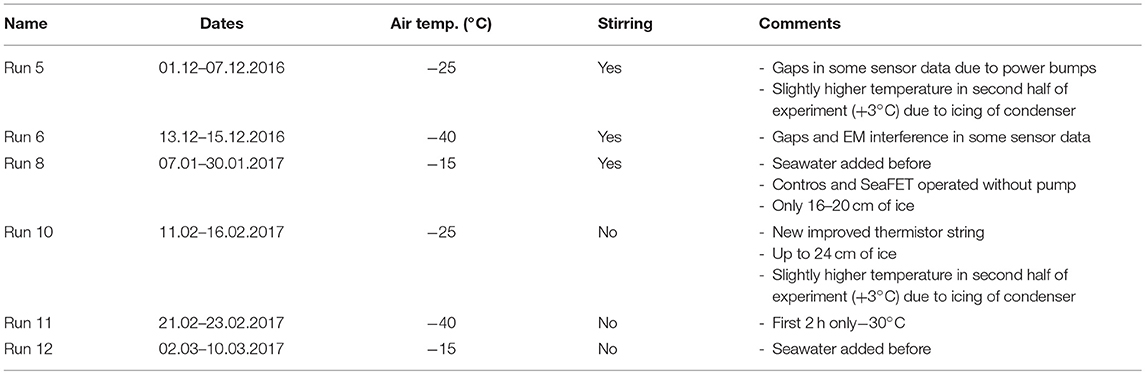
Table 1. Overview of experimental runs.

Water and Ice Melt Samples

In order to calculate a carbon budget, seawater and sea-ice melts were analyzed for TIC content, A_T, and salinity. In addition, the seawater was analyzed for pH.

For each run, water was sampled before the ice formed (“pre-ice” samples), and once the ice had reached a thickness of 20 cm (“under-ice” samples). All pre-ice samples were taken once water temperatures were close to or below 0°C, and while the tank was well-mixed. For some runs, two pre-ice samples were collected to determine the impact of the rapid cooling before each run on the carbon dynamics. For the stirred runs, we collected some pre-ice samples while the water was cooling down relatively quickly, which may have contributed to poor precision between replicates. In the case of the unstirred runs, water was stirred while cooled relatively slowly to about −1°C before pre-ice samples were collected. Only after sampling was the stirring system turned off, and the water left to stratify. For the under-ice samples of these runs, the stirring system was turned on at least 2 h before sampling, to ensure adequate mixing of the stratified water column. For all sampling periods, the sampling port was heated beforehand. In the case of the colder runs, the heating power had to be increased, and the heating period extended. In general, 0.5–2 h of heating was required to open the port and allow sampling. The system was flushed before sampling to remove residual water from the sample port tubing. In the case of under-ice sampling, a significant number of bubbles formed in the sample tubing due to decreased solubility caused by decreased pressure and warming of the water during sampling. While we tried to avoid bubble entrainment during sampling, it could account for some of the differences between replicates sampled during these periods.

Samples were collected in the following order: salinity, TIC and A_T (duplicates), and pH (quadruplicates). In the case of the last three runs, additional salinity samples were collected after TIC and A_T, as salinity appeared to change slightly during the under-ice water sampling (possibly due to some residual stratification in the tank, despite the stirring). Salinity samples were collected into 200 ml borosilicate bottles rinsed three times with sample before filling. Samples for TIC and A_T were tapped into 250 ml borosilicate glass bottles, following a short initial rinse and an overflow of at minimum one bottle volume. Subsequently, the headspace was adjusted, samples were poisoned with 100 μl of saturated mercuric chloride, and the bottles closed using a greased glass stopper and electrician's tape, in accordance with standard operating procedures (Dickson et al., 2007). All TIC and A_T samples were stored in the dark at 4°C before analysis. Samples taken for pH analyses were collected directly into 10-cm spectrophotometric cells, which were rinsed, flushed for approximately 15 s, and closed without a headspace using two Teflon^® stoppers, as described by Dickson et al. (2007). The cells were immediately placed in a 25°C incubator for 1 h before analysis.

Ice cores were collected after the under-ice water sampling and melted for subsequent chemical analyses. For all runs, we took four ice cores from approximately the same locations in the tank (König, 2017), except for Run 6, when only three cores were retrieved. The sampling spots were chosen so that different regions of the tank were sampled to best capture any horizontal variability. The ice was cored manually using a Kovacs Mark II corer (9 cm diameter). After a short visual inspection and determination of core length inside the cold lab (still at the pre-set temperature), the cores were placed in gas-impermeable ALTEF^® bags which were then taken outside the lab and immediately sealed with C-clamps. The bags were closed outside the cold lab, because they became brittle and the clamps were difficult to close at low temperatures. The bags were evacuated immediately after sealing, using a hand-held pump to minimize excessive suction and potential loss of gases trapped inside the core, as suggested by Miller et al. (2015). The cores from the final three experiments were weighed after evacuation so as to determine the ice density, using an Ohaus GT4100 balance.

After evacuation, the cores were placed into a dark container and melted overnight at room temperature. All cores took approximately 24 h to melt completely. Once fully melted, the ice melts were mixed and allowed to warm up until all visible solid particles were dissolved, so as to assure homogeneity. The high reproducibility of TIC and A_T in the ice melt sub-samples (Table S2) confirms that this procedure was indeed adequate. Before sampling the melts, accumulated air inside bags was removed using a syringe. The air volume differed between the melts (ca. 40–200 ml), possibly due to natural heterogeneity, inconsistent evacuation, or, in the case of the highest air volume, a leaky bag or valve leading to uptake of air during melting. However, TIC, A_T, salinity, and the ratios between these parameters were no different in the ice melt sample with the largest air volume (200 ml) than those from the replicate cores without a large head-space. Ice melt samples were sub-sampled by connecting a short Tygon^® tube to the valves of the bags. First, two TIC/A_T samples were tapped, preserved, and sealed like the water samples, except for a slightly smaller overflow (0.5–1 bottle volume) due to the limited ice melt volumes. The rest of the ice melt was used for 1-2 salinity samples, depending on the remaining volume.

Chemical Analyses

Total inorganic carbon was measured coulometrically on a SOMMA system (Johnson et al., 1993), run in combination with a UIC coulometer, using standard operating protocols (Dickson et al., 2007). To ensure the accuracy of the measurements, certified reference materials (CRM batch 152 and 160, provided by Andrew Dickson, Scripps Institute of Oceanography) were measured daily, and all values were corrected accordingly. The analytical precision, calculated from differences between duplicate samples, was about 1 μmol/kg for water samples, and 0.5 μmol/kg for ice melt samples.

Total alkalinity was determined by open cell, potentiometric titration, using a custom built system following the procedure outlined by Dickson et al. (2007). The accuracy of this system was ensured by calibrating against reference materials (CRM batch 152, 160, and 161) at the beginning and end of each day. The analytical precision (determined as for TIC) was about 4 μmol/kg for water samples, and 3 μmol/kg for ice melt samples. Both TIC and A_T analyses were conducted within 4 weeks of collection.

Water sample pH was determined spectrophotometrically within 2 h of collection with an Agilent 8453 spectrometer, using m-cresol purple as an indicator dye, following Dickson et al. (2007). Each absorption measurement was conducted four times and averaged. All values were corrected for a potential pH perturbation by the dye addition. The temperature within the cell was recorded immediately after each spectrophotometric measurement using a hand-held temperature probe (Fluke 5611T). Since some of the under-ice water salinities were outside the range for which the dye pK_a was defined by Clayton and Byrne (1993), pH was calculated (on the free pH scale) following Miller et al. (2011), using the parameterization by Millero et al. (2009). The pH values were then converted back to the total scale using the HSO${}_4^{-}$ acidity constant of Dickson (1990), assuming the sulfate concentrations of the samples were proportional to salinity.

Salinity of water and ice melt samples was determined from conductivity using a Guildline 8400B salinometer, after at least 24 h of acclimatization at the laboratory temperature, which was kept constant at 1°-2°C below the salinometer bath temperature (24°C). The instrument's accuracy was confirmed by the daily measurement of a certified standard (IAPSO Seawater Standard). The salinity analyses were conducted within maximum 6 weeks of collection, and the analytical precision was 0.0003 (on the practical salinity scale).

Carbon Budget

We used a budgetary approach to estimate how TIC in the initial, pre-ice seawater was distributed between the air, water, and ice by the end of each experiment. For this purpose, the absolute TIC content (i.e., moles of carbon) of the formed ice (absTIC_ice) and drained brine (absTIC_drain; calculated from differences in TIC concentration between pre-ice and under-ice water) was compared to the absolute TIC content (absTIC_{sw, ini}) of the volume of seawater which was converted into ice. Any differences between these three values were assumed to originate from exchange with air:

$\begin{array}{l}absTI{C}_{sw,ini}=absTI{C}_{ice}+absTI{C}_{drain}+absTI{C}_{air}\end{array}$

The net TIC exchanged with the air over the course of the experiment (absTIC_air) was thereby not determined directly and could be either positive or negative, as carbon could be released to or taken up from the air, respectively.

To calculate the absolute TIC content of water that eventually froze and the resulting ice, the TIC content measured for the corresponding water (TIC_{sw, ini}) and ice melt samples (TIC_ice), both in μmol/kg, was multiplied by the final ice mass (m_ice), so as to consider only the pre-ice seawater from which the ice had formed. To account for TIC drained from the ice to the under-ice seawater, the difference between the TIC content in pre-ice and under-ice water samples (TIC_{sw, fin} − TIC_{sw, ini}) was multiplied by the total mass of the under-ice water, which was determined by subtracting the final ice mass from the initial water mass (m_sw.ini).

$\begin{array}{l}TI{C}_{sw,ini}\ast m_{ice}=TI{C}_{ice}\ast m_{ice}+(TI{C}_{sw,fin}-TI{C}_{sw,ini})\ast \\ (m_{sw.ini}-m_{ice})+absTI{C}_{air}\end{array}$

The initial water mass was calculated from seawater density, determined from salinity and in-situ temperature according to Millero and Poisson (1981), and the initial water volume based on water depth after sampling and tank dimensions, corrected for estimated sensor volumes (König, 2017). Due to rather large uncertainties regarding ice volume and density, the ice mass was derived from a salinity budget set up in a similar way as the above outlined carbon budget. For this purpose, we replaced the TIC concentrations with the salinities measured in water and ice melt samples in the budget, assuming these practical salinity values represent the mass concentration of salt in water. As we assumed the exchange of salt with air during ice growth to be negligible (thereby neglecting evaporation and sublimation), we set the air fraction of the budget to zero, and could thus determine the ice mass.

The overall uncertainties in the carbon budgets were propagated from analytical errors in TIC and salinity and from estimated errors in the tank volume, seawater density, and sensor volumes. Details of the error analysis are given by König (2017).

Sensors

The sensors installed in the seawater tank with relevance for this study are described in Table 2 and shown in Figure 1B. The three temperature probes were installed at different depths to confirm that the tank was well-mixed, and the majority of the other sensors were installed in the middle of the tank, with an extra pH sensor at the bottom. Dopbeam sonars were deployed at the bottom of the tank. Additional details about sensor configurations during each experiment, including additional sensors installed, are given by König (2017).

TABLE 2

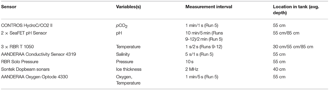
Table 2. Overview of sensors deployed in the seawater tank. Additional sensors installed but not discussed in this paper are described in König (2017).

Sensor CO₂ System

The CONTROS HydroC pCO₂ probe (Fietzek et al., 2014) we deployed was connected to an external pump (SBE 5M, Sea-Bird Scientific) for all experiments except Run 8, when the connection cable to the pump was broken, giving a longer sensor response time for that experiment. The sensor was programmed to zero every 12 h (24 h in the case of Run 8) (Fietzek et al., 2014), and pCO₂ values calculated from pH and TIC of the pre-ice water samples were used to correct for a (generally small) offset in the pCO₂ curve (König, 2017). For pH measurements, we deployed two SeaFET sensors (Martz et al., 2010). As for pCO₂, the pH data were calibrated using the measurements of discrete water samples. Further details about signal correction and data processing are given by König (2017).

Other Parameters

Three RBR TR 1050 probes were installed in the tank at different depths to measure water temperatures. These data were used to check for stratification, correct the SeaFET pH data, and for the sensor CO₂ system calculations. In addition, we obtained temperature data from an O₂ optode (Aanderaa Data Instruments AS, model 4330) deployed in the tank to monitor potential contaminating biological activity.

Seawater salinity was measured by a conductivity sensor (Aanderaa Data Instruments AS, model 4319). This inductive measurement was likely influenced by the sensors and tank walls around it, and therefore, we applied an offset to the data using the discrete water samples (König, 2017).

A pressure sensor (RBR Solo Pressure) was installed in the tank to monitor the potential pressure increase in the water during ice formation and for the CO₂ system calculations. This sensor was calibrated against ambient pressure, as described by König (2017).

Ice Thickness and Brine Release (Dopbeam Sonars)

Three 20 MHz single-beam Dopbeam sonars (Sontek) were deployed in the tank, facing upwards, to survey the growing ice. These sonars record the backscatter of the emitted sonar signal, as well as a velocity profile (Vagle et al., 2012) and were primarily installed to test whether they could provide information on the timing and extent of brine released from the growing ice layer, but we also used them to measure the thickness of the growing ice. This was possible thanks to the density differences between the high-salinity brine, the growing ice, and the underlying water layer, which lead to the reflection of the emitted sonar signals at these interfaces. Further information on the backscatter data collection is given by König (2017).

CO₂ System

The aqueous CO₂ system in the tank was fully characterized using water sample data and the program of van Heuven et al. (2011), with temperature and pressure from sensors deployed in the tank, the borate-to-salinity ratio of Uppström (1974), and KSO₄ dissociation constants of Dickson (1990). Total silicate and phosphate were assumed to be negligible for the calculations. We used the carbonic acid dissociation constants of Cai and Wang (1998), because they gave to the smallest discrepancies between calculated and measured values of the over-determined carbonate system (König, 2017).

We found that after the initial sampling point (before the experiments were started), calculated and measured alkalinity in the water diverged. We suspect that alkalinity was contaminated by an unknown process (possibly electrochemical) associated with the complex configuration of sensors (some of which were new) in the relatively small-volume tank during the initial trial runs. The relative contamination decreased when more seawater was added to the tank. As this A_T increase occurred in a single step at the beginning of our experiments, the relative changes in A_T during each experiment are still useful.

Carbonate system calculations were also conducted with sensor pH (SeaFET 245) and pCO₂ data (HydroC), which allowed us to compute high-resolution TIC and A_T time series. These calculations were only implemented for the stirred runs, since for the unstirred experiments the water was likely stratified, and therefore the sensors did not evaluate the same water.

Results and Discussion

Average Growth Rates

Except at the coldest temperature, the average growth rates were lower for the stirred than the unstirred runs (Table 3), and the largest difference was observed between the slow growth experiments at −15°C. These findings are not surprising, as the stratified water during unstirred runs allowed for quicker freezing due to decreased heat transfer from below. Ice growth during Runs 6 and 11 (coldest conditions, −40°C), appeared to be faster with stirring, but we think this is the result of a delayed start of the main condenser units during the unstirred experiment (Run 11; Table 1), which led to higher temperatures (−30°C) during the first hours of the experiment.

TABLE 3

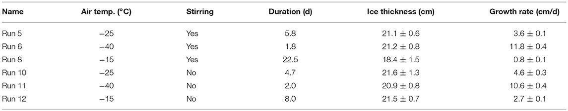
Table 3. Average ice growth rates of all six runs, calculated from the runtime (duration) of each experiment and the average final ice thickness.

Fate of TIC, A_T, and Salinity During Ice Growth

Water and Ice Melt Samples

The relationship between salinity, A_T, and TIC for all water and ice melt samples is illustrated in Figures 2, 3. We included A_T in this analysis, despite the potential contamination (section CO₂ system), since this contamination appeared to be consistent for all discussed runs, and therefore the change in the A_T signal in ice and water can still help identify potential ikaite precipitation in the ice.

FIGURE 2

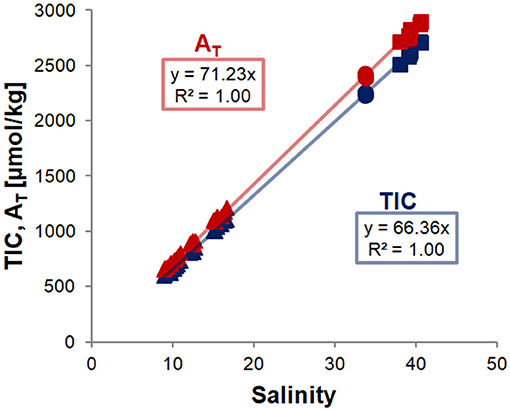
Figure 2. Correlations of TIC (blue) and A_T (red) with salinity in water and ice melt samples of all runs. Replicates of water and ice melt samples were averaged for each sampling point and ice core, respectively, and trend lines were fit through all data points, and forced through zero. Error bars are smaller than the symbols. Analytical data are given in Table S2.

FIGURE 3

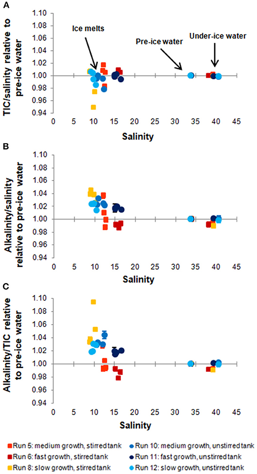
Figure 3. Ratios between TIC and salinity (A), A_T and salinity (B), and A_T and TIC (C) of the sampled ice melts, pre-ice, and under-ice water. For all experimental runs, the data points were normalized to the ratio of the pre-ice water sample, so as to illustrate changes in the ratios during ice growth. Uncertainties were calculated from deviations between replicates.

The excellent fit of the linear regression to the data points in Figure 2 shows that both TIC and A_T are closely coupled with salinity. This indicates that the TIC (and A_T) allocation in the air-ice-water system is strongly dominated by brine processes, and that gas exchange or precipitation processes within the ice are relatively minor. However, closer examination reveals additional differences between the different sample types and experiments (Figure 3). For this comparison, ratios between the variables (e.g., TIC to salinity) were calculated for each data point and subsequently normalized to the ratio of the pre-ice water sample from the same experiment, accounting for dilution (in the case of ice melts) and evaporation effects. For all experiments, changes in the parameter ratios were much more distinct for the ice melt samples than for the under-ice water. Even between ice cores from the same experiment, large discrepancies could be observed, particularly in the stirred runs. The TIC-to-salinity ratio in ice appeared to decrease slightly in most experiments (up to 5% decrease compared to pre-ice water), while A_T seemed to generally increase in the ice, relative to salinity and TIC (increases up to 4 and 9%, respectively). The decoupling of the TIC and salinity signals implies a release of CO₂ from the ice, either to the air above or water below, but through a different mechanism from the salinity release. No significant increase in TIC relative to salinity was identified in the under-ice water, suggesting release to the atmosphere. However, the change in the under-ice water TIC concentration relative to salinity would have been very small, and might have not been detectable within our sampling and analytical uncertainties.

The detected increase in ice melt A_T compared to both TIC and salinity implies precipitation and retention of CaCO₃ minerals (e.g., ikaite) in some of the sampled ice. Since such minerals dissolve during the melting of the ice, they contribute twice as much A_T as TIC to the resulting solution. The observed relative decrease in A_T in some of the under-ice water samples might also be related to this process, as it leads to an increase in TIC (relative to A_T) in the remaining brine, which can then influence the underlying water by drainage (Jones and Coote, 1981). When examining the melting ice cores, white particles, which could have been CaCO₃, were visible for all cores from all experiments. No quantitative analysis of these particles was conducted, and we cannot confirm whether they were indeed CaCO₃ and not some other salt precipitates or contamination. Even though ikaite may have precipitated during all our experiments, its impact on the carbon distribution was small, given the small relative increase in the A_T to TIC ratio in the ice melt samples (mostly less than 5%, apart from one sample with a 10% increase).

Comparing the different experiments, it is difficult to find a clear pattern between the deviations in ice carbonate chemistry and the ice growth rates (Table 3). Nevertheless, it appears as if the A_T to TIC ratio in ice is higher for experiments with slower ice growth (Figure 3C), indicating that CaCO₃ precipitation may be enhanced at slower growth rates. In particular, the experiment with (by far) the slowest ice growth rate displayed an increase in the A_T to TIC ratio in the ice melts of up to 9.4%. This is contrary to expectations of increased ikaite precipitation at lower temperatures/higher brine salinities, but might be caused by the insufficient removal of dissolved CO₂ from the ice during faster ice growth, which is required to achieve ikaite supersaturation (Papadimitriou et al., 2013). The apparent increase in CaCO₃ precipitation at slower ice growth could therefore be related to the increased permeability at these higher temperatures, possibly leading to more efficient removal of CO₂ by outgassing, or simply due to the longer duration of the run, which allowed more CO₂ to escape. This is further supported by pCO₂ values measured in the ice during this run, which were lower than for other runs (König, 2017). Conversely, apparently smaller ikaite precipitation in ice samples in the other runs may simply be due to their shorter runtimes, which may not have been sufficient to allow substantial ikaite precipitation. Papadimitriou et al. (2014) reported that 1–3 weeks, depending on ice temperature, is needed for ikaite precipitation to reach steady state in sea ice.

Despite the generally high A_T in our seawater due to contamination, the absolute A_T to TIC ratios in the ice melt samples of our experiments (average of 1.09 ± 0.02, with a maximum of 1.16) are generally at the lower end of ratios measured in the field, where values of up to 2.2 have been reported (Rysgaard et al., 2007, 2009). However, our values are comparable to those measured in young or newly formed natural and artificial ice (Rysgaard et al., 2007, 2009; Fransson et al., 2015; Geilfus et al., 2016), which further highlights the importance of incubation time for ikaite precipitation. Some ice melts from the two colder, stirred runs (Run 5 and 6) show an inverse pattern from that of the warm run (Run 8), i.e., a relative increase in ice TIC combined with a decrease in A_T. This might have been caused by either increased retention of CO₂ in the ice (e.g., in the form of bubbles), or unidentified deficiencies in sampling and/or analyses. Transport of ikaite from the ice to the underlying water, as suggested by Geilfus et al. (2016), would also explain the relative decrease in ice A_T compared to TIC. However, as no corresponding increase in underwater A_T was detected, and since the permeability in ice was likely too low at our experimental temperatures, we believe this process is not responsible for the relative decrease in ice A_T we detected.

Time Series Variations

While the water samples only provide point measurements at the beginning and end of the experiments, DIC and A_T calculated from sensor pH and pCO₂ allow us to examine changes in the water over the entire experimental period and to compare their development to those of salinity and ice thickness (Figure 4). Comparing TIC, A_T, salinity, and ice thickness (Figures 4A,B), the parameter curves appear to be very similar. At the fastest ice growth rate (Run 6; Figure 4, left column), all four parameters increase nearly linearly over the whole experiment, while for the two experiments at slower ice growth rates, the increase in all three parameters was initially faster and then slowed over the course of the run. It is worth noting that for salinity, the increase was somewhat delayed for all three experiments compared to ice thickness. This was not the case for the TIC and A_T, which appeared to increase even before the surface was ice covered. While an increase in TIC during this period is conceivable due to increased uptake of CO₂ from the air, and has indeed been observed during a similar experiment by Kotovitch et al. (2016), a significant increase in A_T is unrealistic. Furthermore, no such increase was observed for the pre-ice water samples, and it is therefore likely an artifact of the CO₂ system calculations, coupled with the different response times of the sensors. We were only able to estimate the response time for the HydroC sensor and calculations with time-lag corrected sensor data did not provide useful insight (König, 2017).

FIGURE 4

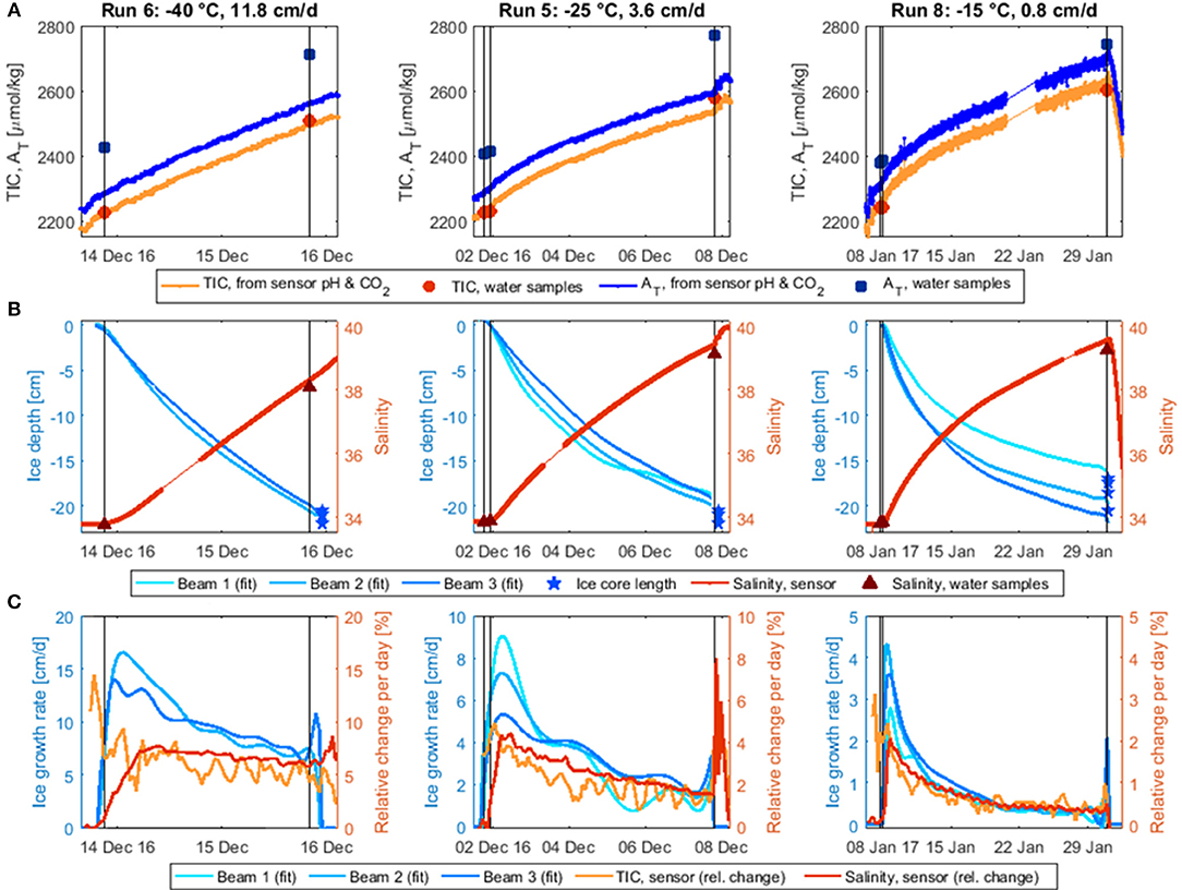
Figure 4. Temporal development of water TIC, A_T (A), water salinity, and ice depth (B; fitted curves from the three Dopbeam sonars) during the three stirred experimental runs as well as the corresponding water sample measurements. TIC and A_T were calculated from the HydroC pCO₂ and the (corrected) external pH of SeaFET 245. Water A_T increased before the experiments started, possibly due to some electrochemical process associated with the sensors and equipment in the tank at initial deployment; note that seawater was added to the tank between runs 6 and 8 (Table 1), reducing the relative impact of the alkalinity contaminant. (C) Ice growth rate (cm/d) derived from Dopbeam-measured ice depth and daily rates of change in salinity (dS/S per day) and TIC (dTIC/TIC per day). Note different vertical and horizontal scales. Black vertical lines indicate water sampling.

To better compare the temporal changes in TIC, salinity, and ice thickness, rates of change were calculated over time intervals adapted to the duration of the run (Figure 4C): 1.5 h for Run 5, 45 min for Run 6, 6 h for Run 8. For TIC and salinity, normalized change rates were calculated, e.g., $d\overline{S}=dS/S,$ using the data curves, which were averaged over the corresponding time interval for this purpose. As the calculated TIC curve was still very noisy, it was further averaged over four adjacent data points. For ice thickness, the change rate (i.e., growth rate) was derived from curve fits to the Dopbeam sonar data.

The ice growth rates decreased significantly over the course of each experiment, due to the insulating effect of the overlying ice (Figure 4C), by more than a factor of five for the slower two experiments and by half for the fastest experiment. Salinity and TIC appeared to increase more steadily over the course of the experiments. This implies a decoupling between ice growth and desalination rates, which can also be observed by comparing the timing of the peak desalination rate, which occurred later than the fastest ice growth rate in all three runs. The discrepancy between peak ice growth and desalination was largest for the fastest ice growth experiment, where the maximum increase in salinity was observed when the ice thickness was 5–6 cm. In the slower two experiments, salinity increased most at ice thicknesses of 0.5–2 cm (Run 8) and 1.5–3 cm (Run 5). These findings are consistent with mushy layer theory, which predicts a delayed onset of brine drainage (Wettlaufer et al., 1997; Notz and Worster, 2009). However, while the peak in the desalination rate appears to be delayed, salinity did begin increasing as soon as the first ice had formed, thereby contradicting the mushy layer predictions. This instantaneous increase could be related to the constant mixing of the tank during these three experiments, which could have disrupted the ice-water boundary layer, as described by Loose et al. (2011).

The rate of change in TIC is harder to interpret, due to the aforementioned difficulties with the sensor CO₂ system calculations, which led to unrealistic increases in A_T and TIC at the beginning of the experiments. Focusing only on the ice growth period (i.e., the time after the last pre-ice water sample was taken), it appears as if TIC was increasing more rapidly than salinity during initial ice growth, but more slowly after that. While this could be an artifact of CO₂ system calculations, it might also be due to a dissimilar behavior of the CO₂ gas and the dissolved salts, as was observed for conservative gas tracers in similar experiments by Loose et al. (2009), who suggested that the differences were related to the faster diffusion of gas away from the ice-water interface. In our case, this process may have been further supported by a slight, additional cooling of the under-ice water (i.e., from approximately −1° to −2°C; König, 2017) and the concomitant increase in gas solubility.

Brine Drainage at Different Growth Rates

The data collected during the experiments without stirring in the tank provide insight into brine release processes, and the temperature dependent differences we observed have potentially important consequences with regard to increasing air temperatures in polar regions. These findings are mainly based on the backscatter data obtained from the Dopbeam sonars, which indeed seemed able to detect brine release from the ice and were further supported by changes in other parameters.

As indicated by the rates of change in the salinity signal (Figure 4C), the maximum desalination from the ice occurred in the early stages of each (stirred) run, but after the maximum ice growth rate had been reached. Similarly, the backscatter signal from the Dopbeam sensors shows a relatively undisturbed, clearly defined ice-water interface up until an ice thickness of about 5–10 cm, after which brine draining out of the ice starts to cloud the strong backscatter signal from the ice, indicating periods of relatively strong brine release (Figure 5A). This delayed onset of the maximum brine drainage is in agreement with predictions of the mushy-layer theory, as discussed above.

FIGURE 5

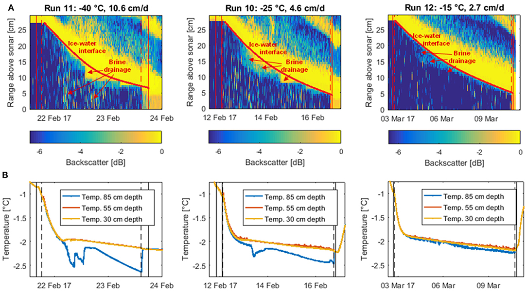
Figure 5. Backscatter profiles (A) and water temperature time series (B) of the three unstirred experiments. The backscatter profiles based on data from the most sensitive Dopbeam sonar were obtained using the difference between the backscatter signal (at each point in time and distance from the sonar) and the maximum backscatter signal of that run. Thus, less negative values indicate stronger backscatter. The strong backscatter signal from the top left to the bottom right corner of each figure represents the descending ice front. The temperature curves were obtained from sensors installed at three different depths in the water, one below the ice (30 cm depth, yellow), one in the middle of the water column (55 cm depth, red), and one at the bottom of the tank (85 cm depth, blue). Solid vertical lines indicate water (and later ice) sampling, dashed vertical lines the switching off (at the start) and on (at the end) of the stirring in the tank.

The blurring of the ice-water interface due to brine drainage is more pronounced for the two coldest experiments, either due to more intense outflow of brine or higher density differences between brine and underlying water, causing a more efficient reflection of the sonar pulses. The notion that brine released during the colder experiments is denser than for the warmer run is further supported by areas of intense backscatter in the water further away from the ice-water interface, as well as temperature measurements in the water column.

While for the warmest unstirred experiment (Run 12), the relatively weak backscatter signal attributed to brine drainage is restricted to the uppermost centimeters of the water column, we find that for the colder two runs, the sonar signal is also scattered back at deeper depths. Furthermore, the temperature signals of sensors installed at three different depths within the water column suggest that during colder runs, the tank was more stratified (Figure 5B). For the colder two runs, abrupt changes in the temperature curve of the bottom sensor coincide with the apparent brine drainage patterns we observed in the backscatter data, suggesting that during the intense brine release period at about 5–10 cm ice thickness, some plumes might have been sufficiently dense to reach the bottom of the tank. No such changes were observed during the warmest run, implying a lack of depth-penetrating brine plumes during this experiment. This finding has potentially far-reaching implications for carbon transport to lower water layers with the so-called “brine pump” (section Implications for future sea ice carbon export, below).

However, as no salinity sensor was deployed at depth, the evidence for more effective vertical brine transport at faster ice growth rates (or colder air temperatures) is circumstantial. Nevertheless, given the potential impact on carbon sequestration of this brine transport, we suggest that further experiments should be conducted with additional probes (as well as in deeper tanks) to resolve the salinity profile across the water column.

Carbon Budget

The results of the carbon budget calculations are shown in Figure 6. For both sets of runs, the majority of TIC (53–72%) was released to the under-ice water, whereas the rest (28–47%) remained in the ice, and exchange with air was negligible. This is in agreement with previous mass balance studies, which found that of all TIC released from the ice, only a small fraction escaped to the air (< 0.1 to 1.1%), while the majority (89.9 to >99.9%) was transported to the underlying water (Nomura et al., 2006; Rysgaard et al., 2007; Sejr et al., 2011). The uncertainty was larger for the air than for water and ice fractions, because the air fraction was estimated from the results of the other fractions. In general, uncertainties in the carbon budget were dominated by the heterogeneity of the ice, which lead to uncertainties in ice TIC and salinity.

FIGURE 6

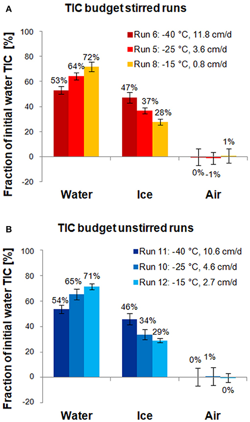
Figure 6. Carbon budgets for stirred runs (A) and unstirred runs (B). Bars show how much of the TIC initially in the water ultimately converted into ice ends up in the final under-ice water, ice, and air, respectively (Section Carbon Budget). Error bars were computed from uncertainties in water and ice TIC, initial water mass, and ice mass (propagated from salinity measurements).

Both stirred and unstirred runs show very similar TIC redistribution patterns: in the fastest ice growth experiments, the ice phase contains nearly half of the initial TIC (47 and 46% for stirred and unstirred runs, respectively) but only less than a third in the slowest growth experiments (28 and 29%, respectively). This is in agreement with expectations that higher growth rates lead to less efficient desalination of the ice, and that TIC largely follows salinity. Carbon budget numbers reported in previous laboratory studies for similar growth rates appear to be in line with the values observed for our experiments (Figure 7).

FIGURE 7

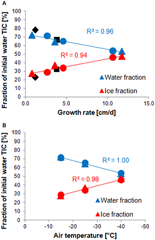
Figure 7. Correlations between the TIC fraction in water (blue) or ice (red) and the average ice growth rate (A) or the ambient temperature (B) of each experiment. Values from stirred runs are marked with round, those from unstirred runs with triangular, symbols. Values measured by previous studies are shown in black, but have not been used for the regression. Black diamonds show values presented by Rysgaard et al. (2007), squares are the (average) results of Nomura et al. (2006). The air temperatures shown in panel B are average values measured during each run, as listed in Table S1.

Interestingly, the TIC redistribution appears to be less dependent on the growth rate than the ambient temperature at which the experiments were run. The slowest experiment (Run 8), for instance, shows a very similar distribution to Run 12, which was run at the same temperature, despite a more than three times lower growth rate. Thus, there is a better (linear) correlation between TIC fractions in water and ice with ambient temperature than with growth rate (Figure 7). Perhaps this reflects the importance of a temperature gradient within the ice in retaining brine and gases.

Implications for Future Sea Ice Carbon Export

Due to large uncertainties in future sea-ice extent and volume (e.g., Meier, 2016; Stammerjohn and Maksym, 2016), meaningful estimates of the total future carbon export from sea ice are difficult. However, the implications of our findings for future potential sea-ice conditions are summarized in Figure 8. In the baseline, “present day” case the majority of TIC released from the sea ice remains in the surface layer, with only a small fraction exported to depth, as predicted in the modeling studies of Grimm et al. (2016) and Moreau et al. (2016).

FIGURE 8

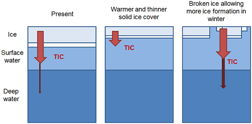
Figure 8. Schematic illustration of the implications of our findings for future scenarios conditions. A thinner and warmer, but complete ice cover and a decrease in total sea ice production leads to a decrease in TIC export to deep water layers. Increased openings within the sea ice cover during winter increase total sea-ice production and export of TIC to deeper water layers.

In cases where warmer air temperatures result in a solid ice cover that is warmer and thinner the expected increase in TIC release (per unit of ice) is canceled out by the decrease in total ice production. Furthermore, export of TIC to the deep ocean is reduced due to the less sufficiently dense brine.

On the other hand, a thinner ice cover also leads to a more mobile, broken ice cover during the winter, with more leads and possibly polynyas. In this case, sea-ice and brine production may actually increase. In addition, that brine and the associated TIC may be exported deeper into the water column, thereby enhancing deepwater formation and carbon sequestration.

It is important to note that these simple future scenarios neglect crucial impacts such as changes to ocean circulation, or the related biological systems. However, they again stress the importance of open water within the sea ice cover, which may not only enhance gas exchange (Loose et al., 2009; Else et al., 2011), but also facilitate export of carbon out of the surface layer (Grimm et al., 2016; this study).

Conclusion and Perspectives

Sea ice growth experiments conducted in a cold laboratory showed that there is a connection between ice growth rates and the redistribution of TIC between the ice and the water underneath. This differential redistribution was evident from discrete water and ice samples, and also visible in continuous time series recorded by underwater sensors. A budgetary approach showed that at higher ice growth rates, relatively more of the initial TIC remains in the ice phase than at slower growth rates (46–47% compared to 28–29%), and the TIC redistribution appeared to depend more on the ambient temperature at which the ice formed than on the ice growth rate. For all experiments, most TIC was rejected into the under-ice water (53–72%, depending on the temperature), while exchange with the air was insignificant, relative to our experimental uncertainties.

The TIC redistribution appeared to be dominated by brine drainage processes, as indicated by a good correlation between TIC and salinity in the ice and water. Minor deviations between the two parameters were likely due to CaCO₃ precipitation in ice and/or CO₂ exchange with the air. Temperature and Doppler backscatter data suggest that whereas more TIC is exported from the ice at higher temperatures (slower ice formation rates), the vertical extent of that transport (e.g., to the bottom of the mixed layer) might be more efficient when ice is formed at colder temperatures (at a faster growth rate). For a more satisfactory assessment of the potential for TIC export to deeper water layers, the stratification and brine release processes should be examined more closely, ideally by the installation of additional salinity probes in the water and possibly the ice.

Data Availability

The data used in this laboratory-based study are included in this manuscript and König (2017).

Author Contributions

DK designed and conducted the experiments with substantial guidance from LM and support from KS. SV provided, installed, and processed the data of the Dopbeam sensors. DK conducted chemical analyses, processed all datasets, and drafted the manuscript. All authors contributed to manuscript editing and revision.

Funding

This project was supported by the Fisheries and Oceans Canada Arctic Sciences Fund. Further financial support was provided by the Zeno Karl Schindler Foundation in the form of a master thesis grant, and by the ETH Zurich Financial Aid Office, which granted a personal travel allowance to DK.

Conflict of Interest Statement

The authors declare that the research was conducted in the absence of any commercial or financial relationships that could be construed as a potential conflict of interest.

Acknowledgments

We would like to thank the staff of the Institute of Ocean Sciences for their support, especially Kenny Scozzafava and Jasmine Wietzke for salinity analyses, Marty Davelaar for help with the TIC and alkalinity analyses, and Sarah Zimmermann and Jonathan Velarde for help with ice coring. Further thanks are due to Nicolas Gruber for his support during the master's thesis this paper is based on, and to him and his group, as well as the BEPSII community for all the fruitful discussions during the preparation of this manuscript.

Supplementary Material

The Supplementary Material for this article can be found online at: https://www.frontiersin.org/articles/10.3389/feart.2018.00234/full#supplementary-material

References

Anderson, L. G., Falck, E., Jones, E. P., Jutterström, S., and Swift, J. H. (2004). Enhanced uptake of atmospheric CO₂ during freezing of seawater: a field study in Storfjorden, Svalbard. J. Geophys. Res. Oceans 109:C06004. doi: 10.1029/2003JC002120

CrossRef Full Text | Google Scholar

Barber, D. G., Ehn, J. K., Pućko, M., Rysgaard, S., Deming, J. W., Bowman, J. S., et al. (2014). Frost flowers on young Arctic sea ice: the climatic, chemical, and microbial significance of an emerging ice type. J. Geophys. Res. Atmos. 119, 11593–11612. doi: 10.1002/2014JD021736

CrossRef Full Text | Google Scholar

Cai, W.-J., and Wang, Y. (1998). The chemistry, fluxes, and sources of carbon dioxide in the estuarine waters of the Satilla and Altamaha Rivers, Georgia. Limnol. Oceanogr. 43, 657–668. doi: 10.4319/lo.1998.43.4.0657

CrossRef Full Text | Google Scholar

Clayton, T. D., and Byrne, R. H. (1993). Spectrophotometric seawater pH measurements: total hydrogen ion concentration scale calibration of m-cresol purple and at-sea results. Deep Sea Res. Part I Oceanogr. Res. Papers 40, 2115–2129. doi: 10.1016/0967-0637(93)90048-8

CrossRef Full Text | Google Scholar

Cox, G., and Weeks, W. (1975). Brine Drainage and Initial Salt Entrapment in Sodium Chloride Ice. CRREL Res. Rep. 345., Hanover, NH: U.S. Army Cold Regions Research and Engineering Laboratory.

Google Scholar

Dickson, A. G. (1990). Standard potential of the reaction: AgCl(s) + 1/2 H₂(g) = Ag(s) + HCl(aq), and the standard acidity constant of the ion HSO₄ in synthetic sea water from 273.15 to 318.15 K. J. Chem. Thermodyn. 22, 113–127. doi: 10.1016/0021-9614(90)90074-Z

CrossRef Full Text | Google Scholar

Dickson, A. G., Sabine, C. L., and Christian, J. R. (eds.). (2007). Guide to Best Practices for Ocean CO2 Measurements. Sidney, BC: North Pacific Marine Science Organization, PICES Special Publication 3.

Google Scholar

Eicken, H. (1992). Salinity profiles of Antarctic sea ice: field data and model results. J. Geophys. Res. Oceans 97, 15545–15557. doi: 10.1029/92JC01588

CrossRef Full Text | Google Scholar

Else, B. G. T., Papakyriakou, T. N., Galley, R. J., Drennan, W. M., Miller, L. A., and Thomas, H. (2011). Wintertime CO₂ fluxes in an Arctic polynya using eddy covariance: evidence for enhanced air-sea gas transfer during ice formation. J. Geophys. Res. Oceans 116:C00G03. doi: 10.1029/2010JC006760

CrossRef Full Text | Google Scholar

Feltham, D. L., Untersteiner, N., Wettlaufer, J. S., and Worster, M. G. (2006). Sea ice is a mushy layer. Geophys. Res. Lett. 33:L14501. doi: 10.1029/2006GL026290

CrossRef Full Text | Google Scholar

Fietzek, P., Fiedler, B., Steinhoff, T., and Körtzinger, A. (2014). In situ quality assessment of a novel underwater pCO₂ sensor based on membrane equilibration and NDIR Spectrometry. J. Atmosph. Oceanic Technol. 31, 181–196. doi: 10.1175/JTECH-D-13-00083.1

CrossRef Full Text | Google Scholar

Fransson, A., Chierici, M., Abrahamsson, K., Andersson, M., Granfors, A., Gardfeldt, K., et al. (2015). CO₂-system development in young sea ice and CO₂ gas exchange at the ice/air interface mediated by brine and frost flowers in Kongsfjorden, Spitsbergen. Ann. Glaciol. 56, 245–257. doi: 10.3189/2015AoG69A563

CrossRef Full Text | Google Scholar

Geilfus, N.X., Carnat, G., Dieckmann, G. S., Halden, N., Nehrke, G., Papakyriakou, T., et al. (2013). First estimates of the contribution of CaCO₃ precipitation to the release of CO₂ to the atmosphere during young sea ice growth. J. Geophys.Res. Oceans 118, 244–255. doi: 10.1029/2012JC007980

CrossRef Full Text | Google Scholar

Geilfus, N. X., Galley, R. J., Else, B. G. T., Campbell, K., Papakyriakou, T., Crabeck, O., et al. (2016). Estimates of ikaite export from sea ice to the underlying seawater in a sea ice–seawater mesocosm. Cryosphere 10, 2173–2189. doi: 10.5194/tc-10-2173-2016

CrossRef Full Text | Google Scholar

Gough, A. J., Mahoney, A. R., Langhorne, P. J., Williams, M. J. M., and Haskell, T. G. (2012). Sea ice salinity and structure: a winter time series of salinity and its distribution. J. Geophys. Res. Oceans 117:C03008. doi: 10.1029/2011JC007527

CrossRef Full Text | Google Scholar

Griewank, P. J., and Notz, D. (2013). Insights into brine dynamics and sea ice desalination from a 1-D model study of gravity drainage. J. Geophys. Res. Oceans 118, 3370–3386. doi: 10.1002/jgrc.20247

CrossRef Full Text | Google Scholar

Grimm, R., Notz, D., Rysgaard, S., Glud, R., and Six, K. D. (2016). Assessment of the sea ice carbon pump: insights from a three-dimensional ocean-sea-ice biogeochemical model (MPIOM/HAMOCC). Elementa 4:000136. doi: 10.12952/journal.elementa.000136

CrossRef Full Text | Google Scholar

Johnson, K. M., Wills, K. D., Butler, D. B., Johnson, W. K., and Wong, C. S. (1993). Coulometric total carbon dioxide analysis for marine studies: maximizing the performance of an automated gas extraction system and coulometric detector. Marine Chem. 44, 167–187. doi: 10.1016/0304-4203(93)90201-X

CrossRef Full Text | Google Scholar

Jones, E. P., and Coote, A. R. (1981). Oceanic CO₂ produced by the precipitation of CaCO₃ from brines in sea ice. J. Geophys. Res. Oceans 86, 11041–11043. doi: 10.1029/JC086iC11p11041

CrossRef Full Text | Google Scholar

König, D. (2017). Carbon Dynamics during the Formation of Sea Ice at Different Growth Rates. Master thesis, Swiss Federal Institute of Technology Switzerland.

Kotovitch, M., Moreau, S., Zhou, J., Vancoppenolle, M., Dieckmann, G. S., Evers, K.-U., et al. (2016). Air-ice carbon pathways inferred from a sea ice tank experiment. Elementa 4:000112. doi: 10.12952/journal.elementa.000112

CrossRef Full Text | Google Scholar

Loose, B., McGillis, W. R., Schlosser, P., Perovich, D., and Takahashi, T. (2009). Effects of freezing, growth, and ice cover on gas transport processes in laboratory seawater experiments. Geophys. Res. Lett. 36:L05603. doi: 10.1029/2008GL036318

CrossRef Full Text | Google Scholar

Loose, B., Miller, L. A., Elliott, S., and Papakyriakou, T. (2011). Sea ice biogeochemistry and material transport across the frozen interface. Oceanography 24, 202–218. doi: 10.5670/oceanog.2011.72

CrossRef Full Text | Google Scholar

Martz, T. R., Connery, J. G., and Johnson, K. S. (2010). Testing the honeywell Durafet® for seawater pH applications. Limnol. Oceanograp. Methods 8, 172–184. doi: 10.4319/lom.2010.8.172

CrossRef Full Text | Google Scholar

Meier, W. N. (2016). “Losing Arctic sea ice: observations of the recent decline and the long-term context,” in Sea Ice, ed D. N. Thomas (Chichester: John Wiley), 290–303.

Google Scholar

Miller, L. A., Carnat, G., Else, B. G. T., Sutherland, N., and Papakyriakou, T. N. (2011). Carbonate system evolution at the Arctic Ocean surface during autumn freeze-up. J. Geophys. Res. Oceans 116:C00G04. doi: 10.1029/2011JC007143

CrossRef Full Text | Google Scholar

Miller, L. A., Fripiat, F., Else, B. G. T., Bowman, J. S., Brown, K. A., Collins, R. E., et al. (2015). Methods for biogeochemical studies of sea ice: the state of the art, caveats, and recommendations. Elem. Sci. Anth. 3:000038. doi: 10.12952/journal.elementa.000038

CrossRef Full Text | Google Scholar

Millero, F. J., DiTrolio, B., Suarez, A. F., and Lando, G. (2009). Spectroscopic measurements of the pH in NaCl brines. Geochim. Cosmochim. Acta 73, 3109–3114. doi: 10.1016/j.gca.2009.01.037

CrossRef Full Text | Google Scholar

Millero, F. J., and Poisson, A. (1981). International one-atmosphere equation of state of seawater. Deep Sea Res. Part A. Oceanogr. Res. Papers 28, 625–629. doi: 10.1016/0198-0149(81)90122-9

CrossRef Full Text | Google Scholar

Moreau, S., Vancoppenolle, M., Bopp, L., Aumont, O., Madec, G., Delille, B., et al. (2016). Assessment of the sea-ice carbon pump: Insights from a three-dimensional ocean-sea-ice biogeochemical model (NEMO-LIM-PISCES). Elem. Sci. Anth. 4:000122. doi: 10.12952/journal.elementa.000122

CrossRef Full Text | Google Scholar

Moreau, S., Vancoppenolle, M., Delille, B., Tison, J.-L., Zhou, J., Kotovitch, M., et al. (2015). Drivers of inorganic carbon dynamics in first-year sea ice: a model study. J. Geophys. Res.Oceans 120, 471–495. doi: 10.1002/2014JC010388

CrossRef Full Text | Google Scholar

Nakawo, M., and Sinha, N. K. (1981). Growth rate and salinity profile of first-year sea ice in the high arctic. J. Glaciol. 27, 315–330. doi: 10.1017/S0022143000015409

CrossRef Full Text | Google Scholar

Nomura, D., Granskog, M. A., Fransson, A., Chierici, M., Silyakova, A., Ohshima, K. I., et al. (2018). CO₂ flux over young and snow-covered Arctic pack ice in winter and spring. Biogeosciences 15, 3331–3343. doi: 10.5194/bg-15-3331-2018

CrossRef Full Text | Google Scholar

Nomura, D., Yoshikawa-Inoue, H., and Toyota, T. (2006). The effect of sea-ice growth on air–sea CO₂ flux in a tank experiment. Tellus B 58, 418–426. doi: 10.1111/j.1600-0889.2006.00204.x

CrossRef Full Text | Google Scholar

Notz, D., and Worster, M. G. (2009). Desalination processes of sea ice revisited. J. Geophys. Res. Oceans 114. doi: 10.1029/2008JC004885

CrossRef Full Text | Google Scholar

Papadimitriou, S., Kennedy, H., Kennedy, P., and Thomas, D. N. (2013). Ikaite solubility in seawater-derived brines at 1 atm and sub-zero temperatures to 265 K. Geochim. Cosmochim. Acta 109, 241–253. doi: 10.1016/j.gca.2013.01.044

CrossRef Full Text | Google Scholar

Papadimitriou, S., Kennedy, H., Kennedy, P., and Thomas, D. N. (2014). Kinetics of ikaite precipitation and dissolution in seawater-derived brines at sub-zero temperatures to 265 K. Geochim. Cosmochim. Acta 140, 199–211. doi: 10.1016/j.gca.2014.05.031

CrossRef Full Text | Google Scholar

Parmentier, F.-J. W., Christensen, T. R., Sorensen, L. L., Rysgaard, S., McGuire, A. D., Miller, P. A., et al. (2013). The impact of lower sea-ice extent on Arctic greenhouse-gas exchange. Nature Clim. Change 3, 195–202. doi: 10.1038/nclimate1784

CrossRef Full Text | Google Scholar

Petrich, C., and Eicken, H. (2016). “Overview of sea ice growth and properties,” in Sea Ice, ed D. N. Thomas (Chichester: John Wiley), 1–41.

Google Scholar

Rysgaard, S., Bendtsen, J., Delille, B., Dieckmann, G. S., Glud, R. N., Kennedy, H., et al. (2011). Sea ice contribution to the air–sea CO₂ exchange in the Arctic and Southern Oceans. Tellus B 63, 823–830. doi: 10.3402/tellusb.v63i5.16409

CrossRef Full Text | Google Scholar

Rysgaard, S., Bendtsen, J., Pedersen, L. T., Ramløv, H., and Glud, R. N. (2009). Increased CO₂ uptake due to sea ice growth and decay in the Nordic Seas. J. Geophys. Res. Oceans 114:C09011. doi: 10.1029/2008JC005088

CrossRef Full Text | Google Scholar

Rysgaard, S., Glud, R. N., Sejr, M. K., Bendtsen, J., and Christensen, P. B. (2007). Inorganic carbon transport during sea ice growth and decay: a carbon pump in polar seas. J. Geophys. Res. Oceans 112:C03016. doi: 10.1029/2006JC003572

CrossRef Full Text | Google Scholar

Sejr, M. K., Krause-Jensen, D., Rysgaard, S., Sørensen, L. L., Christensen, P. B., and Glud, R. N. (2011). Air–sea flux of CO₂ in arctic coastal waters influenced by glacial melt water and sea ice. Tellus B 63, 815–822. doi: 10.1111/j.1600-0889.2011.00540.x

CrossRef Full Text | Google Scholar

Stammerjohn, S., and Maksym, T. (2016). “Gaining (and losing) Antarctic sea ice: variability, trends and mechanisms,” in Sea Ice, ed D. N. Thomas (Chichester: John Wiley), 261–289.

Google Scholar

Stephens, B. B., and Keeling, R. F. (2000). The influence of Antarctic sea ice on glacial–interglacial CO₂ variations. Nature 404:171. doi: 10.1038/35004556

PubMed Abstract | CrossRef Full Text | Google Scholar

Tison, J.L., Haas, C., Gowing, M. M., Sleewaegen, S., and Bernard, A. (2002). Tank study of physico-chemical controls on gas content and composition during growth of young sea ice. J. Glaciol. 48, 177–191. doi: 10.3189/172756502781831377

CrossRef Full Text | Google Scholar

Uppström, L. R. (1974). The boron/chlorinity ratio of deep-sea water from the Pacific Ocean. Deep Sea Res. Oceanogr. Abstracts 21, 161–162. doi: 10.1016/0011-7471(74)90074-6

CrossRef Full Text | Google Scholar

Vagle, S., Gemmrich, J., and Czerski, H. (2012). Reduced upper ocean turbulence and changes to bubble size distributions during large downward heat flux events. J. Geophys. Res. Oceans 117:C00H16. doi: 10.1029/2011JC007308

CrossRef Full Text | Google Scholar

van Heuven, S. D., Pierrot, J. W. B., Rae, E. L., and Wallace, D. W. R. (2011). MATLAB Program Developed for CO2 System Calculations. Oak Ridge, Tennessee: U.S. Department of Energy, Carbon Dioxide Information Analysis Center, Oak Ridge National Laboratory.

Google Scholar

Vancoppenolle, M., Meiners, K. M., Michel, C., Bopp, L., Brabant, F., Carnat, G., et al. (2013). Role of sea ice in global biogeochemical cycles: emerging views and challenges. Quat. Sci. Rev. 79, 207–230. doi: 10.1016/j.quascirev.2013.04.011

CrossRef Full Text | Google Scholar

Wettlaufer, J., Worster, M. G., and Huppert, H. E. (1997). Natural convection during solidification of an alloy from above with application to the evolution of sea ice. J. Fluid Mech. 344, 291–316. doi: 10.1017/S0022112097006022

CrossRef Full Text | Google Scholar