 Desmond Manatsa1,2*
 Geoffrey Mukwada1
- 1Afromontane Research Unit, Geography Department, Free State University, Bloemfontein, South Africa
- 2Geography Department, Bindura University of Science, Bindura, Zimbabwe
The Brewer–Dobson circulation (BDC), whose dynamic activity is enhanced from winter to spring, transports stratospheric ozone from the tropical source regions to higher latitudes. But it is the BDC's shallow branch which transfers lower stratospheric ozone (LSO) from the tropics to the subtropics. Hence the accumulation of ozone in the subtropics is at its maximum at the end of spring (October) in the Southern Hemisphere (SH). Here we use observation and observation constrained reanalysis data to investigate the extent to which the interannual variability of this end of spring accumulated LSO is able to impact on the maximum surface air temperature (SATmax) and precipitation of South Africa. This is achieved through contrasting years of high positive and negative October ozone anomalies for the extreme BDC activity, referred to as weak (wBDC) and strong (sBDC) respectively. It is found that the w(s)BDC event composites coincide with significant negative (positive) SATmax anomalies and positive (negative) rainfall over South Africa. We suggest that the wBDC's related LSO surpluses trap the UVB meant to heat the troposphere and surface. This induces the observed negative middle to upper tropospheric air temperatures and geopotential heights resulting in cyclonic circulation anomalies that enhances rainfall and suppresses SATmax. The opposite is true for the sBDC composites where ultimately the elevated geopotential heights result in middle to upper anticyclonic tropospheric anomalies that are accompanied by rainfall deficits and increased SATmax.
Introduction
The ozone composition, especially in the upper troposphere lower stratosphere (UTLS) is influenced by tropical upwelling (Yulaeva et al., 1994; Randel et al., 2007; Konopka et al., 2010; Young et al., 2011) and subtropical/extratropical downwelling across the tropopause layer (Gettelman et al., 2011; Shepherd and McLandress, 2011) through the stratosphere troposphere exchange process (STE, Holton et al., 1995; Randel et al., 2009; Calvo et al., 2010). Both vertical and meridional stratospheric ozone transport are largely controlled by the wave driven Brewer Dobson Circulation (BDC) whose strength is mainly measured by Elliassen Palmer flux (EPf, Randel et al., 2002; Konopka et al., 2010). As such, a rough sketch of the BDC involves tropical upwelling of mass from the troposphere (source regions) to the stratosphere (Gerber, 2012), the mean meridional mass transport in the stratosphere that is accompanied by downwelling of mass in the subtropics and extratropics through distinct shallow and deep branches respectively (Birner and Bönisch, 2011; Ueyama et al., 2013; Konopka et al., 2015). The shallow branch mostly results from wave forcing in the subtropical UTLS (Abalos et al., 2014; Konopka et al., 2015), while the deep branch is predominantly influenced by high-latitude planetary waves (Ueyama et al., 2013; Abalos et al., 2014; Konopka et al., 2015). Of interest here is the shallow branch as it does not only present a dynamical forcing within the UTLS where the bulk of the stratospheric ozone resides (Brunner et al., 2006; Kirgis et al., 2013) but has relatively much faster transport times (Bönisch et al., 2011; Flury et al., 2013). However in the UTLS the lifetime of ozone is comparable to or longer than transfer time scales, making ozone concentration strongly influenced by transport (Kirgis et al., 2013). Hence the shallow branch of the BDC exerts a major influence on the distributions of UTLS ozone which is essential in modulating the penetration of ultraviolet radiation (UV) to the troposphere and surface (WMO Scientific Assessment of Ozone Depletion, 2014). This means that the composition of ozone in the tropics that is meridionally moved by the BDC should have an effect on the vertical ozone concentration over the tropics. As such the accompanying ozone-UV related variability has potential to significantly impact on South Africa's temperature, both in the troposphere and surface.
Nevertheless, stratospheric ozone is predominantly determined by in situ creation (production), destruction (loss) and transport into or out of the region (Kirgis et al., 2013). But unlike in the UTLS where ozone concentration is largely affected by transport (Bencherif et al., 2007, 2011; El Amraoui et al., 2010), photochemical formation and destruction dominate the upper stratosphere, the region of pronounced manmade ozone-depleting substances (ODS) effects (UNEP United Nations Environment Programme, 1999). These ODSs have also contributed to the changes in global ozone levels where the upper stratospheric ozone decline has been more apparent from 1979 (Kirgis et al., 2013). Hence, the discovery of a spectacular austral springtime chemical depletion of Antarctic ozone due to the ODS whose spatial extent of significant ozone loss has been popularly christened the “ozone hole” a few decades ago (Solomon et al., 1986; Molina and Molina, 1987). This phenomenon has since been the most topical environmental issue of the 20th century where the related UVB impact has been demonstrated to adversely affect human health, agriculture and natural ecosystems (Sharma, 2001). The heightened concern on the UVB impact led to the first environmental global treaty known as the Montreal Protocol (MP) whose aim is to regulate the ODS emissions. However, the resounding success of this global treaty is thought to have halted the accelerated global ozone depletion from the mid 1990s (Egorova et al., 2013). As a result, no significant upward trend has been observed in global ozone since 1997 (Steinbrecht et al., 2009; Eckert et al., 2014). But recent studies put more emphasis on atmospheric dynamics as the most likely cause of the observed alterations in the total ozone column (TOC) since the late 1990s, with contribution from the decline in the ODS only being insignificant (Wohltmann et al., 2007). Of late Ball et al. (2018) revealed tropical ozone loss that is primarily confined to the lower stratosphere from 1998, which interestingly, coincides with the global energy imbalance (Trenberth et al., 2014). Although a detailed attribution to specific causal mechanisms is not apparent, this observation may provide a clue on a possible link between the LSO depletion and the warming of the troposphere and surface.
The annual cycle of tropical ozone and temperature in the lower stratosphere is reasonably well understood and is known to result from the annual variation in tropical upwelling and the action of the BDC (Yulaeva et al., 1994; Randel et al., 2007; Konopka et al., 2010; Young et al., 2011). The associated deep tropical convection is capable of rapidly feeding ozone deficit tropospheric air into higher ozone abundances of the lower stratosphere through the STE process (Randel et al., 2009; Calvo et al., 2010) thereby diluting the ozone layer. Hence increased upwelling has been suggested as an explanation for LSO decreases (Weber et al., 2003; Eckert et al., 2014). In fact, significant negative trends in the tropical LSO, dominated by increased tropical upwelling, has been observed in the last two decades (Randel and Thompson, 2011; Abalos et al., 2013; Sioris et al., 2014) which has been related to the global warming induced acceleration in the BDC (Garcia and Randel, 2008; Shepherd and McLandress, 2011; Butchart, 2014). But the LSO has a simultaneous direct radiative effect that affects temperature not only in the lower stratosphere but is also inversely related to the air temperature and hence geopotential heights of the troposphere below (Randel et al., 2017). As such it is highly possible that the BDC-shallow branch's related dynamical perturbations at subtropcal latitudes can directly influence the variability of ozone and temperature (Nath and Sridharan, 2015) including the temperature induced air circulation over South Africa.
In this regard, we investigate the extent to which interannual variability in the LSO due to the shallow braches of the BDC is able to affect the maximum surface air temperature (SATmax) and rainfall over South Africa. We do this by contrasting years of high positive and negative October ozone anomalies when the winter-spring cumulative ozone totals from the BDC activity is at its maximum, hereafter referred to as weak (wBDC) and strong (sBDC) respectively. This comparison, however, is made possible by assuming that the anomalies caused by the external forcing resulting from the ozone extremes is significantly larger than the one attributed to internal processes. This is not farfetched as several recent studies which specified non-zonal ozone forcings were able to demonstrate significant surface response to LSO variability (e.g. Gillett et al., 2009; Waugh et al., 2009).
Data and Methods
We predominantly employ observation and observation constrained reanalysis data through statistical means to provide evidence on the BDC link to the surface temperature and precipitation over South Africa for the month of October. The month of October is when ozone variability is at its maximum and hence so is the LSO-UV modulation over the region. Observations have the advantage that they are independent from the presumed underestimation of the calculated energy in the UV solar spectrum (Ward, 2016). The main atmospheric parameters analyzed were temperature and TOC. This is because temperature is associated with a unique ozone radiative property in which the lower stratospheric temperature (LST) is inversely related to the tropospheric air temperature directly below (Randel et al., 2017). However, its limitation is that it includes other processes that might have different influences on ozone-temperature response like water vapor (Kirk-Davidoff et al., 1999). For the surface temperature analysis, we used a station observation-based global land monthly mean surface air temperature dataset at 1°C latitude–longitude resolution comprising of both maximum and minimum from Berkeley Earth (Muller et al., 2013). The TOC is from a single coherent dataset of the Royal Netherlands Meteorological Institute, derived from the multi-sensor reanalysis version 2 (KNMI MSR2). This dataset provides global assimilated ozone fields spanning from 1979 to present based on 14 satellite datasets (van der et al., 2015). For verification purposes of the TOC, we used the Total Ozone Mapping Spectrometer (TOMS) dataset (McPeters et al., 1998). However, we did not exclusively use this dataset to verify all the analysis duration as the TOC data is provided freely to the public only up to 2007. In any case, the TOMS ozone data correlate very well with the KNMI MSR2 ozone, which leaves no doubt that the observed ozone variations in this work, were real.
The interpretation of the TOC vertical temperature response is drawn from the National Centers for Environmental Prediction (NCEP)–National Center for Atmospheric Research (NCAR) reanalysis (NCEP; Kalnay et al., 1996). Although compared to the more modern ERA-Interim, which has been found to perform better on daily time scales over Southern Africa (Moalafhi et al., 2017), the NCEP has been found to perform equally good on monthly time scales (Manatsa et al., 2013, 2015). Vertically, NCEP also provides a good agreement with radiosonde data after 1979, the period that corresponds to the introduction of satellite data into the reanalysis assimilation scheme (Marshall, 2003). In this regard, the readily available NCEP dataset, which predominantly uses observations and extend higher into the lower stratosphere, provides a more consistent vertical model based pattern relative to the surface. The lower stratosphere is considered as the vicinity of the tropopause (70–100-hPa layer) which is the location of the ozone layer, where not only the largest ozone fraction (~90%) of the TOC is found (Steinbrecht et al., 1998; Brunner et al., 2006; Kirgis et al., 2013) but the associated ozone changes are primarily driven by atmospheric dynamics (Abalos et al., 2014). In this regard, the TOC measurements predominantly reflect the LSO distribution (Kirgis et al., 2013) and as such are strongly correlated (Steinbrecht et al., 1998; Manatsa et al., 2013). Therefore, we represent the LSO with TOC which henceforth is referred to simply as “ozone.” The ozone hole index is created from ozone hole data that is downloaded from http://www.theozonehole.com/ozoneholehistory.htm.
The strength of the BDC is not an easily observable quantity and hence is rather a difficult parameter to measure (Gerber, 2012; Ball et al., 2016). Several studies have attempted to estimate empirically the variability of the BDC using the lower-stratospheric (~100 hPa) Eliassen–Palm (EP) flux (Hood and Soukharev, 2005; Konopka et al., 2015), temperature (Yulaeva et al., 1994; Ueyama and Wallace, 2010; Young et al., 2011) and geopotential height data (Chandra et al., 1996; Hood et al., 1997) and even the out of phase changes between the tropical and subtropical ozone (Randel et al., 2002) as effective proxies. But the subtropical interannual ozone variability in winter/spring can be attributed to wave-induced changes in the BDC (Hood and Soukharev, 2005). In fact Randel and Thompson (2011) noted that the tropical LSO is so closely tied to tropical upwelling that they considered it an “excellent” proxy for upwelling. Hence we expect the subtropical ozone buildup in winter and spring to be significantly influenced by interannual variations in the BDC. This entails that the related ozone variability over subtropical South Africa can be seen as a reasonable measure of the strength of the overall BDC. Since the BDC has a more pronounced signal in the month-to-month and interannual variability (Young et al., 2011), in this work we use the monthly ozone amounts over South Africa to infer the strength of the BDC. Because we are principally interested in determining the influence of the BDC induced LSO on the lower troposphere and surface temperature, the strength of the BDC is inferred from the area-averaged ozone values in the boxed region (21, 30° E and 27°S, 31°S) which is presented by a box in Figure 2A. It is also from this region that the ozone, tropospheric lower temperature (TLT) and SATmax time series were derived that are represented by SA_ozone, SA_TLT and SA_SATmax where the prefix SA stands for South Africa.
Pearson correlation method is applied to account for linear relationships. But to show the independent influence of each variable, a partial correlation technique is used as explained by (Behera et al., 2005). Basically this involves approximating the exclusive connection between two variables while linearly excluding the influence arising from another independent variable (Behera et al., 2005). The use of the composite analysis was principally to detect the most salient and dominant characteristics contained within the selected group of events. Correlations and the mean differences in the composites are considered to be statistically significant at the 95% and 90% confidence levels respectively, based on the standard two-tailed Student's t-test. Prior to doing any statistical operation, all the data are detrended so as to remove the presumed linear influence of greenhouse gas-induced global warming. All the indices consist of monthly (October) values per year, hence as expected, no robust autocorrelation on the time series is detected (e.g., Manatsa et al., 2013). In this regard, the impact of autocorrelation in significant hypothesis testing is rendered non-essential. The post satellite period from 1979 to 2017 was selected for analysis because that is the period when the data coverage improved significantly. The anomalies were computed by subtracting the current World Meteorological climatological mean of 1981–2010 from each of the time series considered.
In order to detect abrupt changes/shifts, we adopted a manually performed cumulative sum (CUSUM) technique (Wetherill and Brown, 1991), as it performs robustly and is relatively easy to execute (Breaker, 2007; Manatsa and Mukwada, 2017). The analysis of cumulative variables where the cumulative sum of a variable has to be preferred to the variable itself as a measure of performance in climate research has recently gained credibility (Heim et al., 2017; Partanen et al., 2017; Graf and Tomczyk, 2018). This emanates from the realization that certain climate driven variables do not only respond instantaneously but also to the accumulated effects over the period of time (Manatsa et al., 2015). In this regard, the CUSUM method enables the shift process to be considered holistically, being composed of sequenced and linked events rather than monthly events that are independent (Manatsa and Mukwada, 2017). We also used the Sequential Regime Shift Detector (SRSD, Rodionov and Overland, 2005) in order to confirm the derived shifts and ascertain their p-values.
The empirical orthogonal function (EOF) analysis, also known as the principal component (PC) analysis (Jolliffe, 2002) was the preferred technique to define the dominant modes of the October gridded SATmax variability. The EOF basically generates new variables by way of linear combinations of the original ones, which explain most of the variance in the observed data. This technique has the advantage that it is able to simultaneously extract the dominant temporal variability and the associated spatial homogeneity. The former mode of variability is normally referred to as the PC while the latter is termed the EOF. Its algorithm is provided by the Climate Explorer website (http://www.temis.nl/protocols/o3field/o3mean_msr.php). However, its limitation is that the spatial patterns of leading EOFs have a certain degree of dependence on the shape of the analysis domain whereby the mode either ceases to exist or changes when the domain is altered. Worse still, the technique assumes orthogonality which is a property rarely found in physical systems of the climate. In any case, despite these seemingly major shortcomings, the classical EOF analysis remains popular in climate research. Here we used the EOF analysis with the aim to underline the hypothesis that regional October South Africa's SATmax and TLT are essentially influenced by the BDC induced LSO variations.
Results
Composites Representing the WBDC and SBDC and the 1997 Shift
While the BDC activity drives the ozone which in turn acts on temperature within the lower stratosphere, it is not an easily observed quantity (Gerber, 2012; Ball et al., 2016). In this regard we use the verified strong temperature response to ozone as a natural and simple way to identify the variability of the BDC (Yulaeva et al., 1994; Ueyama and Wallace, 2010; Young et al., 2011) and the related impact on the surface temperature below. Thus, in order to establish the coherency of the ozone–temperature relationship over South Africa, the ozone anomalies are arranged in descending order alongside their corresponding SA_SATmax anomalies as shown in Figure 1A. In this way we found it easy to identify extreme ozone anomaly event years together with their corresponding SA_SATmax anomalies. As such, there are 7 positive (negative) extreme ozone anomaly-years identified by blue (red) lines. These 7 year events for each composite are chosen because they have undergone the largest October ozone anomaly (broken line) related BDC amplitudes [greater than an arbitrarily chosen magnitude of 7.0 Dobson Units (DU)] with respect to the adopted current World Meteorological Organization (WMO)'s mean period (1981–2010). The accompanying inversely connected SA_SATmax anomalies are shown in blue and red bars that are designated as weak-BDC (wBDC) and strong-BDC (sBDC) composites comprising of the years (1981; 1991; 1989; 1979; 2017; 1984; 1988) and (2003; 2015; 2004; 1997; 2008; 2006; 1985) respectively. Interestingly, it can be noted that all, except 2017(1985) of the w(s)BDC events occurred before(from) 1997.
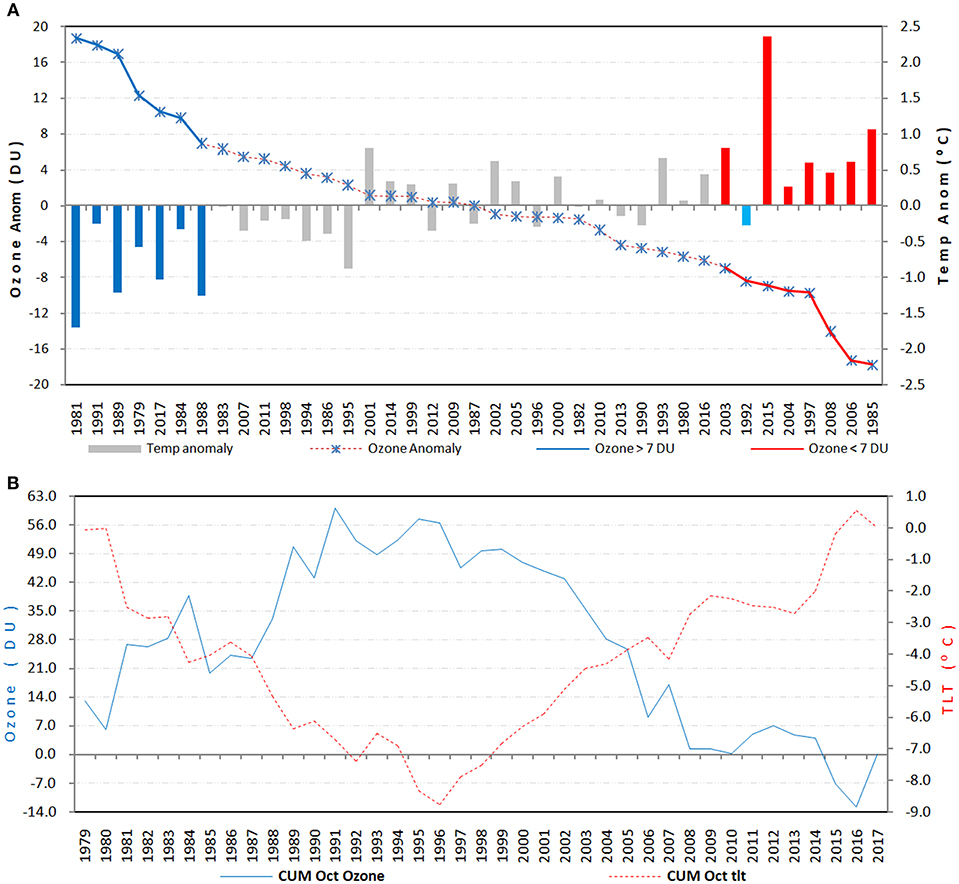
Figure 1. (A) Temporal manifestation for the SA-ozone anomaly (DU) that is arranged in descending order (broken line with asterisks) with the corresponding SA_SATmax anomalies (°C). Blue (red) bars represent SA_SATmax anomalies matching the extreme ozone anomalies that are greater (less) than 7 DU while gray bars stand for those with smaller magnitudes. The light blue bar amongst the red bars is the year 1992 which we considered an outlier. (B) The CUSUM time series for October ozone (broken red line) alongside that of October TLT (solid blue line). The data are for October from 1979 to 2017.
From Figure 1A we also note that the year 1992 (light blue bar) can be considered an outlier within the sBDC composites. This suppressed SA_SATmax could be associated with the sulfate aerosol impacts following the eruption of Mt. Pinatubo that was found to be largely confined to the lower stratosphere (Randel et al., 2009; Young et al., 2011). Sulfurous gases emitted by volcanoes convert to sulfate aerosols in the stratosphere whose concentration is dramatically enhanced for longer periods following major volcanic eruptions. These have a huge impact on the Earth's radiative balance where they increase the reflection of incoming solar radiation and increase the infrared absorption which cools the Earth's surface and the troposphere, while warming the stratosphere (Solomon et al., 2016). In fact the Mt Pinatubo eruption impact years (1992, 1993, 1994, and 1995) including that from El Chichón years (1982, 1983, 1984) show a distinct mismatch (Polvani et al., 2017) between the expected ozone amount and the corresponding SA_SATmax response in Figure 1A. In this regard, the exclusion of these seven years appears to produce an increase in the strength of the anticorrelation between the SA_ozone and SA_SATmax from −0.727 to −0.877 though this was not statistically detectable from the p-values which essentially remained < 0.0001 for the 2 cases. As a result, it appears major volcanic eruptions degrade the relationship between the LSO and SATmax over South Africa.
Additionally, the importance of decadal variability in shaping the overall trends in SA_ozone and SA_TLT, especially in revealing a possible shift in the temporal manifestations both time series is necessary. As such we use the CUSUM technique to locate any discontinuity which could be hidden in the time series. The use of this method did not only reveal a common shift around 1997 but also further cements the proposed notion of the cause effect inverse relationship between the two parameters (Figure 1B). This shift point was confirmed using the SRSD (Rodionov and Overland, 2005) with a p < 0.0001 for SA_TLT but 0.0092 for SA_ozone. Interestingly the year 1997 has also become the standard shift point in most of the research involving the LSO long term trends and hence demarcates the two epochs often used to investigate the distinctly reversing ozone trends (e.g., Manatsa et al., 2013; Harris et al., 2015; Polvani et al., 2017). SA_SATmax, though not presented in the figure, also displays a shift around the same period. This should be expected as SA_SATmax and SA_TLT are strongly correlated at p < 0.0001 hence suggesting that both temperature indices could be responding to ozone variability.
The Connection of SATmax to Ozone Variability Over South Africa
In order to approximate the region of maximum SATmax variability together with its associated temporal manifestation over the subtropical South Africa (south of 23° S), we employ an EOF analysis on the gridded SATmax (Figure 2A). Table 1 shows the resulting modes of variability retained which have been truncated to 4 upon reaching the cumulative explained variance of 93.36%, using the screeplot method. It can be noted that the dominant mode of SATmax explained variance of EOF1 and EOF2 accounts for 63.86 and 22.08% respectively. But because of the relatively high values for these adjacent modes, we then used the North et al. (1982) criterion to show that they are independent at 95% confidence level. North et al. (1982) technique is usually used to determine significance of the separation of the neighboring EOFs. With such a dominating percentage of representation, we assume that the EOF1 and PC1 are able to represent reasonably well the spatiotemporal variability of SATmax over South Africa. However, we could not relate EOF2 and the other subsequent modes to any known physical processes and as such ignored discussing them further.
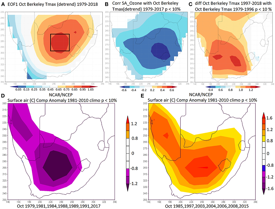
Figure 2. The spatial pattern of (A) SATmax_EOF1 with the boxed region demarcating the location where the averaged values of the indices were derived from, (B) correlation between SA_ozone index and SATmax, (C) mean difference between SATmax of the 1997–2017 and 1979–1996 epochs and surface mean temperature composite for (D) wBDC and (E) sBDC. All the data are for October from 1979 to 2017 and the significance (colored shades) is for 90% confidence level using the 2 tailed t-test.

Table 1. Explained variance of SATmax (detrended) of southern Africa south of 23°S.
On correlating the SA_SATmax index with ozone over the South African region, we note that the area demarcated with maximum correlation values in Figure 2B largely coincides with the central parts of South Africa that is predominantly occupied by the Free State Province. The mean difference SATmax map in Figure 2C, which essentially depicts the difference between the sBDC and wBDC composites, emphasizes the turnaround to warming that is confined to the subtropical region associated with the post shift ozone depletion period. Again the composites of the SATmax in Figures 2D,E confirm the subtropical restriction of the surface temperature where the s(w)BDC event composites are associated with positive (negative) anomalies. On the overall, it can be noted through visual inspection that the area of high EOF amplitudes has a strong resemblance with the spatial patterns presented in the w(s)BDC composites depicted in Figures 2D,E. This may indicate that the variability of the LSO may not only be involved in generating the observed spatial patterns but could also be directly linked to the dominant mode of SATmax variability over South Africa.
Impact of Ozone on Lower Tropospheric and Surface Temperature Over South Africa
It is because of the BDC's well-known seasonality that it becomes reasonable to demonstrate the temporal evolution of the BDC extreme events using the composite analysis. In this regard, we present in Figure 3A, the monthly sequence from January to December of the ozone related sBDC and wBDC respective events with the aim to differentiate the distinct temporal evolution of the two extreme composite events from the neutral BDC events. In this figure it can be appreciated that in general the ozone values start to increase from a summer (DJF) minimum through winter (JJA) to attain a spring (SON) maximum, but with a spike in October (Young et al., 2011). This monthly ozone variability is consistent with other studies (Thompson et al., 1996; Sivakumar and Ogunniyi (2017) who noted that over South Africa the monthly variation of ozone concentration show maximum and minimum concentrations during spring and autumn, respectively. That the LSO is lowest in autumn but highest during spring is itself most likely the consequence of the stronger tropical tropospheric upwelling in austral summer/autumn compared to austral winter/spring (Young et al., 2011). This mechanism brings more ozone poor air from the troposphere to dilute the lower stratosphere which in turn is transported to the subtropics by the shallow branch of the BDC. The reverse occurs during the cool season of limited convection. Consequently, this meridionally transported LSO accumulates in the subtropics to reach maximum amounts at the end of spring. Hence it can be implied that the most likely explanation for subtropical South Africa's monthly ozone amplitudes presented in Figure 3A, is the strength of the BDC activity which has a winter and spring hemispheric maximum (Hood and Soukharev, 2005; Young et al., 2011). Thus, in order to appreciate the BDC extreme activity influence on ozone concentration we also present in Figure 3A, the monthly ozone amplitudes for the composites of the wBDC and sBDC with the broken line representing the neutral BDC events. It can be noted that significant deviations from the mean start to manifest themselves from June with maximum differences being realized in October after which they abruptly fall to insignificance again a month later from November. In this regard, the observation that the LSO concentration is suppressed for sBDC but enhanced for wBDC is itself a predominant consequence of stronger tropical upwelling during the former composites compared to the latter. In this regard, the BDC displays both interannual and decadal significant variability especially the considerable strengthening during the recent two decades that was attributed to global warming (Garcia and Randel, 2008; Butchart, 2014). Hence this may explain the highly increased frequencies of the pre (post) 1997 shift w(s)BDC events which were revealed in Figure 1A.
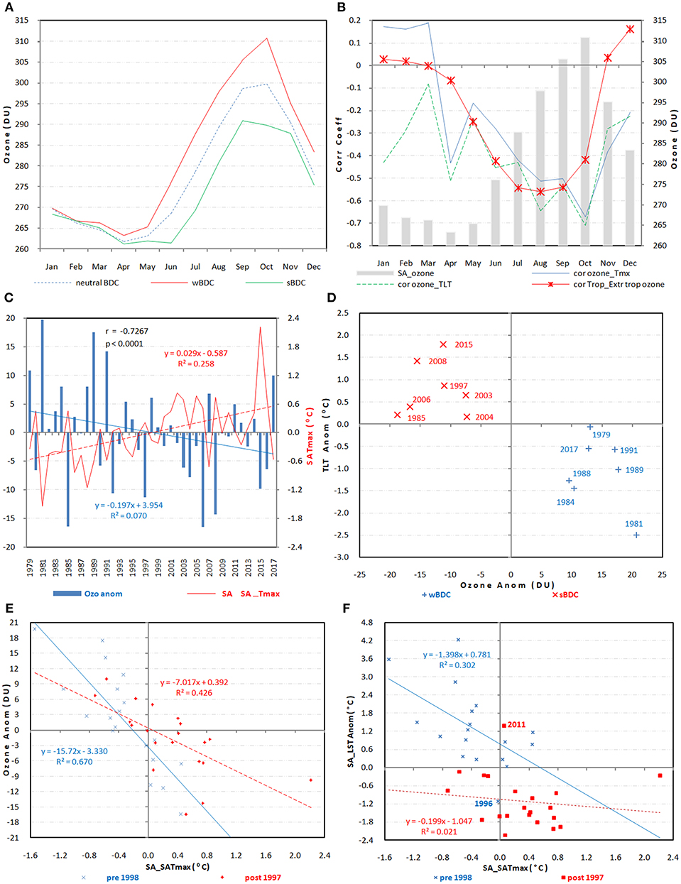
Figure 3. Monthly (A) SA_ozone anomalies related to the wBDC, sBDC, and neutral BDC composites and, (B) correlation values between SA_ozone and SA_SATmax (blue line), SA_ozone and SA_TLT (green line) that is superimposed on the monthly correlated values between the tropically and subtropically averaged ozone (red line with asterisks). In the background are the monthly ozone values for the wBDC composite (gray bars). (C) Temporal manifestation of SA_ozone anomalies alongside that of SA_SATmax with the corresponding regression lines superimposed. (D) October scatter plot for SA_TLT anomalies (° C) against SA_ozone anomalies (DU) for the wBDC (blue crosses) and sBDC (red crosses). The scatterplot for (E) SA_SATmax against SA_ozone and (F) stratospheric temperature anomalies against SA_SATmax. In the inserts of the figures are the regression line equations. The data is for the post satellite period of 1979 to 2017.
A strong radiative response due to LSO variability in the troposphere is a well-known phenomenon (Previdi and Polvani, 2014 and references therein). In this respect, we present in Figure 3B the monthly correlation of SA_ozone with SA_SATmax, and SA_TLT juxtaposed against the highest monthly amplitudes as exemplified by the wBDC composite. By exploiting the out of phase nature of the tropical—subtropical LSO as demonstrated in previous studies relating LST to the BDC (Young et al., 2011) we present the monthly evolution of the correlation coefficients between the tropically and subtropically averaged ozone (red line with asterisks in Figure 3B). Here it is realized that the tropical and subtropical averaged ozone are significantly negatively correlated (p < 0.1) during austral winter and spring, suggesting that variations in wave driving are a major factor controlling global-scale ozone variability in the lower stratosphere. This allowed us to infer the monthly strengths of the BDC at global scale. Since the SA_ozone has a cumulative buildup, it can be appreciated that as the ozone amplitudes increases, so does the strength of the correlation coefficients between SA_ozone with SA_TLT and SA_SATmax. As expected, the correlations reach maximum values in October when ozone accumulation is at its highest. Although the graph is not shown, the correlation with SATmin is considerably weaker with the its maximum strength being attained a month later in November. This implies that the strongest simultaneous temperature responds of ozone at monthly time scale is again achieved in October but with surface SA_SATmax and SA_TLT. That is why October has become the month of focus as it does not only display maximum ozone values but also the strongest simultaneous coupling with both the lower tropospheric and surface maximum temperatures. Since SA_SATmax and SA_TLT display a simultaneous correlation which is close to unity (0.892, p < < 0.0001) this suggests that these temperature variables either respond to the same stimuli or strongly influence one another. But the greatest values of SA_SATmax and SA_TLT are attained in the afternoon (Yang and Slingo, 2001) implying that the ozone connection with temperature could be a direct response to solar radiation. In fact, (Young et al., 2011) demonstrated that the seasonal cycle in the LST and LSO are strongly in sympathy with the annual march of insolation.
In this regard we display in Figure 3C, the temporal manifestation of monthly ozone values alongside the surface temperature response. Here we see that the two variables are significantly inversely related with a correlation of −0.727 (p < 0.0001). Figure 3C also indicates that the magnitudes of the monthly amplitudes are strongly inversely corresponding. This further suggests the simultaneous nature of the SA_SATmax and SA_TLT response to the ozone variability. In any case, it appears the SA_ozone (SA_SATmax) anomaly amplitudes are higher and positive (negative) before the 1997 shift than after where the inverse corresponding pattern of anomalies seem to have been suppressed. In fact the SA_ozone (SA_SATmax) pre-shift average has significantly shifted from 302.98 DU (18.01°C) to 294.726 DU (18.98°C) with a p-value of 0.048 (0.018). The inserted oppositely signed regression line trends suggest that the reduction in SA_ozone feeds into the increasing SA_SATmax. However, the declining trend in SA_ozone, though not significant is inconsistent with the Antarctic ozone which was found to have either stabilized or slightly increased thereby either reversing or arresting the ozone hole expansion in the recent decades as a result of the MP related reductions in the emissions of ODS (Solomon et al., 2016). Actually the expectation is that the global ozone mean should increase as the ODS continue to decline (Eckert et al., 2014). This inconsistency could be an indication that the cause of SA_ozone variability is largely detached from the chemical ozone depletion related to the ozone hole. In fact the signs of ozone recovery related to the decline in the stratospheric halogen loading were predominantly observed in the upper stratosphere where the effects of the ODSs are easily quantifiable (UNEP United Nations Environment Programme, 1999). But in the tropical lower stratosphere, statistically significant negative trends which were detected (Randel and Thompson, 2011; Ball et al., 2018) could be attributed to systematically increased tropical upwelling that is easily represented in simulations of several chemistry climate models (Eyring et al., 2007; Shepherd, 2007; Li et al., 2009; Waugh et al., 2009). Similarly in the subtropics, the dominant contribution to the TOC was found to be due to the larger influence from atmospheric dynamics related to the BDC on the LSO (Newchurch et al., 2003; Steinbrecht et al., 2009).
The distinct nature for the relationship between the SA_TLT and SA_ozone as imposed by the sBDC and wBDC composites is depicted in the scatter plot in Figure 3D. Here it is quite evident that the connection occupies the first and third quadrants, which is a good sign of the separation of the two composites as far as influencing temperature is concerned. Since a coinciding 1997 shift for both SA_TLT and SA_ozone has been revealed in Figure 1B, we demonstrated in the scatter plot (Figure 3E) that the relationship between the two time series shows less post shift SA_ozone corresponding to higher temperatures accompanied by a weaker coupling. This is supported by the correlation coefficient r between the SA_SATmax and SA_ozone for the two epochs which suggests significantly reduced correlation in the latter epoch (R2 = 0.670 compared to R2 = 0.426). The same conclusions also apply to Figure 3F where the significant pre-shift R2 of 0.346 drops to an insignificant value of 0.020. However, from this figure it can further be noted that the pre-shift mean LST has cooled significantly from −59.18°C to −61.69°C with a 2-tailed t-test p-value for the difference between the means of < < 0.0001. Though explaining the reasons is beyond the scope of this work, the same figure also reveals that 2011(1996) is the only post(pre)-shift event with positive(negative) LST anomalies but with corresponding SA_SATmax that is not anomalous. Since ozone is by far the dominant temperature forcing in the lower stratosphere (Forster and Shine, 1997), the anomalous LSO therefore connects to the temperature in the troposphere and surface. As such the connection weakens as the ozone becomes depleted. Hence over the subtropics, where South Africa is largely located, it is most likely that the enhanced action of the BDC has predominantly contributed to the ozone loss in the lower stratosphere (Newchurch et al., 2003; Steinbrecht et al., 2009) which coincide with higher surface temperatures.
Link of SATmax Variability to the BDC
Of late it has been confirmed that the LSO together with surface temperatures display a BDC induced near-perfect cancellation between tropical and extratropical latitudes on both annual and interannual time scales (Gettelman et al., 2010; Young et al., 2011; Abalos et al., 2012). In fact the inter-annual variations seen in the subtropics TOC anti-correlate with that in the tropics (Figure 3B red line with asterisks) as a result of the overturning BDC (Young et al., 2011; Abalos et al., 2012; Zhou et al., 2012). Hence in order to demonstrate the dynamical ozone variability associated with the lower branch of the BDC, it becomes prudent to establish the existence of this anticorrelation spatial pattern between these respective latitudinal bands. This is done through correlating PC1_SATmax and SA_ozone with the ozone and SATmax in the SH respectively. Hence, in Figures 4A,B, it can be realized that these indices generate inverse spatial bands of tropical and extratropical significant correlation values. In fact the 20°S−20°N and 40°S−50°S zonal bands of significant correlations in these two figures are within the BDC shallow branch's upwelling and downwelling regions respectively. These are indicative of the zones related to ozone exhaustion and accumulation respectively during the poleward meridional transport. As such this spatial pattern merely manifests the characteristic SH springtime LST response to BDC-ozone related forcing (Salby, 2008; Grise and Thompson, 2013). It is interesting to note that an October BDC index which we derived from the differences between the averaged TOC in the tropics and the subtropics (Randel et al., 2002) that we demonstrated in Figure 3B (red line with asterisks) has a unique impact on Africa's SATmax that is confined only to South Africa (Figure 4C). This demonstrates the regional confinement of the BDC's impact on the African continent which we are revealing in this work.
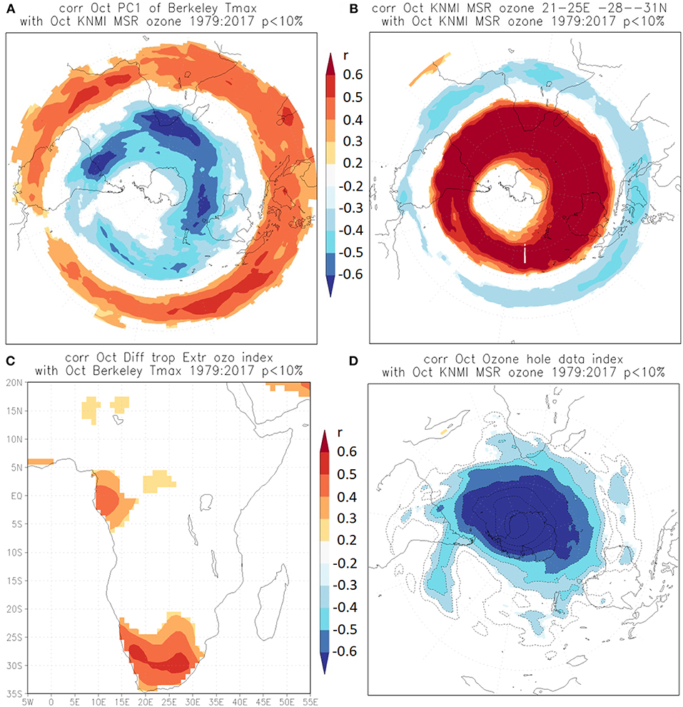
Figure 4. Spatial manifestation of (A) correlation field between SAT_PC1 and the SATmax over the SH, and (B) SA_ozone and the ozone over the SH. (C) The spatial correlation between the tropics minus subtropics ozone averaged index and the SATmax over Africa. (D) correlation of ozone hole index with ozone over the SH. The data is from October from 1979 to 2017. Color shades depict regions of significance that is above the 90% confidence level using a 2 tailed t-test.
The chemical and BDC induced dynamical ozone modulating processes, though not fully independent of one another, are the two possible causal mechanisms for LSO trends and interannual variability in the subtropics (Hood and Soukharev, 2005). Chemical processes that may contribute to subtropical ozone decreases are related to the increase in ODSs that is known to be the main cause of ozone declines in the polar regions (Solomon et al., 1986, 2016; Molina and Molina, 1987). As such, the dynamically induced, in the absence of polar chemistry induced ozone anomalies however, may not entirely explain the ozone anomalies over South Africa. At times the ozone hole has been observed to be quite elliptical, with the axis running from the Antarctic Peninsula toward the southwest of South Africa (http://www.theozonehole.com/2016ozonehole.htm). This implies that the polar vortex can influence heterogeneous chemical ozone loss over this region. For example, the polar vortex itself has been found to affect mid-latitude ozone levels through the ozone dilution process, i.e., mixing of polar ozone-poor air with mid-latitude ozone-rich air (Hadjinicolaou and Pyle, 2004). In this respect, one would be tempted to believe that the variations of ozone over South Africa is predominantly a result of the encroachment of the ozone hole influence as the variability is also significantly linked to the Antarctic ozone hole data as shown in Figure 4D. Hence in order to discredit this notion as the possible explanation of dominant SA_ozone loss, we employ the partial correlation method as used in (Behera et al., 2005). In this technique the influence due to ozone hole can be linearly removed from the intended relationship and similarly that of SA_ozone can also be excluded. The results show that when the effects due to ozone hole are linearly removed, the correlation between SA_ozone and SA_SATmax is not significantly altered as it changes from −0.633 to −0.584 and retains the p < 0.001. But when that from SA_ozone is similarly removed, from the correlation between SA_SATmax and ozone hole index, the relationship drastically collapses, falling from a significant (p < 0.01) value of 0.418 to an insignificant (p = 0.329) correlation of 0.275. In this regard though it is not physically possible to entirely disentangle the dynamic from the chemical ozone loss mechanisms, we underplay the role of the latter in favor of the former as the predominant mechanism for the ozone depletion over South Africa. This can also be inferred from Figure 3C where the exhibited high ozone variability is most probably due to dynamics rather than halogen loading whose chemical ozone loss evolves more smoothly (Kirgis et al., 2013). As such chemical ozone loss is unlikely the main mechanism involved in the w(s)BDC ozone related changes.
Ozone Link to Vertical Air Temperature Patterns Using the wBDC and sBDC Composites
The signal of the shallow branch of the BDC in terms of ozone anomalies from the tropics to the sub-tropics can be inferred in the UTLS where the vertical movement of ozone predominates through the tropopause. GHGs can be discounted since they do not have an impact that is confined to the UTLS (Polvani et al., 2017). As such the UTLS is where the steepest relative vertical ozone gradients are found (Abalos et al., 2013), hence the corresponding large vertical gradients in the air temperature that we see in the plates of Figure 5. In these figures we observe almost simultaneous cooling (heating) of the lower stratosphere and heating (cooling) of the troposphere and surface. This concurrent inverse temperature response which is insignificantly related to surface temperature advection (figure not shown) is most likely a result of radiative forcing emanating from above that is related to ozone variability. Hence, it becomes prudent to analyze the related vertical air temperature stratification. In this regard, the vertical slices of the w(s)BDC air temperature composites are shown in Figures 5A–D. Figures 5A,C depict the meridional slice averaged between 21°E and 25°E which strands from 20°N southwards to 45°S so that the both tropical regions can be connected to South Africa. The meridional slice passes through the boxed region illustrated in Figure 2A but has been chosen to cut through the region of maximum tropospheric circulation response. However, the stronger temperature response in both the subtropical stratosphere and surface compared to the tropics for w(s)BDC composites should be the result of more accumulation (depletion) of the LSO richer (poorer) air due to the general impact of the slower (quicker) meridional transport from the tropics.
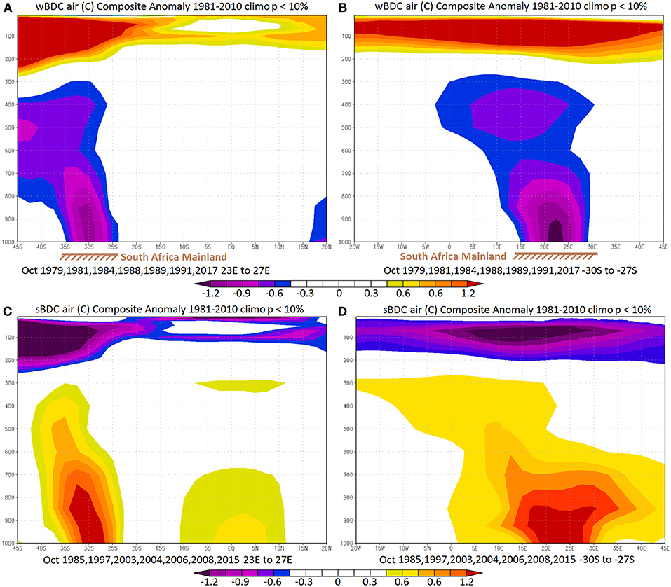
Figure 5. Vertical air temperature pattern for the wBDC composites averaged over (A) 21°E to 25°E and extending from 40°S to 20°N, (B) 33°S to 30°S and covering 20°W to 45°E (C,D) same as in (A,B) respectively but for sBDC composites. Years for the composites are indicated in the insert and were derived from October data spanning from 1979 to 2017. The anomalies are with respect to the 1981-2010 climatology. Shaded regions are significant above the 90% confidence level.
The sun's output of UVB, at the analyzed timescale does not significantly change. Rather the more the ozone, the more the high energy absorption in the lower stratosphere and hence the less the UVB is available to heat the troposphere and the Earth's surface. In Figures 5B,D, the region of maximum temperature response in the lower stratosphere corresponds to that in the upper troposphere and surface directly below. Since tropospheric upwelling is directly related to air temperature, it is to be expected that weaker (stronger) subtropical upwelling should be found in the w(s)BDC composites. Hence, this necessitates anomalous accumulation (depletion) of ozone in the lower stratosphere as a result of relatively less (more) intrusion of tropospheric ozone deficit air in the w(s)BDC composites. Due to greater (reduced) UVB radiation allowed through the lower stratosphere, it follows that the s(w)BDC composites are associated with more(less) temperature response both in the troposphere and surface. However, more ozone in the lower stratosphere increases the temperature sensitivity as it traps increased UVB that is destined to filter through the tropopause. In this regard, the dipole atmospheric temperature patterns depicted in the plates of Figure 5 should most likely be predominantly the radiative effect of the LSO variability in the presence of UVB (Randel et al., 2009) rather than adiabatic processes as envisaged by Ball et al. (2016).
Interestingly, all plates in Figure 5 emphasize both the significant role of the subtropics and the restriction to the continental impact in modifying the vertical configuration of the wBDC and sBDC air temperature composites due to the differential absorption of UVB. The land surface skin is heated much faster to initiate a more anomalous convection and hence tropospheric upwelling than the ocean as the UVB penetrates deeper into the ocean to use the heat over a thicker layer. In this respect, the coinciding LST minimum (maximum) with the surface temperature maximum (minimum) over the subcontinent suggests a positive feedback mechanism between the boundary layer and the ozone (e.g., Olsen et al., 2007). Although this has to be confirmed through experiments, we propose that the BDC anomalies for strong (weak) phases during early spring generates land surface warming (cooling) which is accompanied by enhanced (suppressed) tropospheric upwelling. Hence this should result in the LSO being further depleted (accumulated) during the sBDC (wBDC) phases which then may increase(decrease) the UVB radiation allowed to anomalously warm (cool) both the troposphere and surface.
Significant tropospheric response is mainly confined to the continental surface of South Africa. The temperature response occurs with different magnitudes in the boundary layer and free lower troposphere as compared to the upper troposphere. In this regard, the boundary layer seem to respond more to the surface heating whist the upper troposphere appear to respond more to temperature changes in the lower stratosphere. This is confirmed by the high correlation between the SA_SATmax and the SA_TLT which is about 0.892 (p < < 0001) and hence implying that both troposphere and surface are heated from the same source which is probably the solar UVB. However, the surface has the lowest (highest) temperature values that are directly below the region of lowest (highest) lower stratospheric air temperature anomalies in Figures 5B,D. This is also an indication that the highest anomalous UVB has the strongest impact on the surface temperature below where the high energy is absorbed with some of it being reflected to heat the boundary layer immediately above. The higher temperature anomalies in the upper troposphere relative to the middle troposphere may signify ozone temperature response to the amount of UVB allowed to enter the troposphere, where ozone is in more abundance in the upper part (Brunner et al., 2006). In fact relative to these atmospheric layers, South African springtime ozone maximum has been found in both the lower stratosphere and upper troposphere (Thompson et al., 1996; Sivakumar and Ogunniyi, 2017). As such, the stratospheric cooling(warming) juxtaposed against tropospheric (cooling) observed in October is thus primarily a response to ozone extreme alterations (Randel et al., 2009). In any case, the LSO -induced cooling (warming) in the upper troposphere can be reproduced in the current generation of coupled atmosphere–ocean general circulation models (GCMs) and coupled chemistry–climate models (CCMs; Young et al., 2013).
Circulation Anomaly Patterns Associated With the wBDC and sBDC Composites
The assumption of a cause-and-effect relationship between the stratospheric ozone and tropospheric circulation is not novel. It is on record that anticyclonic related subsidence anomalies are characterized by deformations of the subtropical tropopause resulting in protrusions of ozone-poor, low potential vorticity air that extend from the subtropical upper troposphere into the lowermost stratosphere (Waugh and Polvani, 2000). The reverse process generates tongues of ozone-rich stratospheric air extending into the subtropical upper troposphere (Waugh and Polvani, 2000). In this way, once developed the upper tropospheric anomaly circulations are bound to enhance the inverse relationship in ozone anomalies that have been indicated in the troposphere and lower stratosphere. In fact Barodka et al. (2015) used a “top-down” approach to demonstrate the impact of the LSO on tropospheric circulation patterns and the associated weather and climate conditions. Figure 6A shows the warming of the LST juxtaposed against tropospheric cooling that has maximum response vertically aligned from the lower stratosphere, upper and then lower troposphere to the surface for the wBDC composites over South Africa. We also represent, for the same composites, in Figures 6B,C the truncated the geopotential and the corresponding zonal circulation respectively, that is restricted to the troposphere because the atmosphere is a lot denser with the controls of the surface climate easily noticeable there than in the stratosphere. These composites indicate that when the upper part of the troposphere is cooled coinciding with the LSO surplus related warming (also presented in Figures 5A,B), the geopotential height responses by falling with maximum values in the upper part as depicted in Figure 6B. This in turn creates a low pressure anomaly system in the upper troposphere where the wind anomaly becomes strongly cyclonic (Figure 6C). We illustrate in Figure 6D that the wBDC composite for the upper tropospheric air temperature anomalies depict a center that largely coincides with the region of maximum circulation anomaly pattern presented in Figure 6E. It then becomes easy to spatially link these air temperature anomaly systems to the cyclonic winds that are quite vivid in Figures 6C,E. Hence this cyclonic wind system should be responsible for the significant positive rainfall anomalies presented in Figure 6F as the associated ascending motion which should be more pronounced from the lower middle levels of the troposphere is conducive to cloud development of large vertical extent. It is however important to observe that the precipitation anomalies are enhanced more to the east of the low pressure system covering most of the central regions of South Africa (mostly Free State Province) which is predominantly in the northerly components of the winds circulating the low pressure anomaly. This could be an indication that the source of the moisture is of tropical origin. It can also be implied that this resulting enhanced rainfall further cools the near surface, through evaporation, which is evidenced in Figures 5B, 6A. In the same vein, it appears that the predominantly arid region to the south of the box demarcated in Figure 2A may benefit from the positive rainfall anomalies shown in Figure 6F.
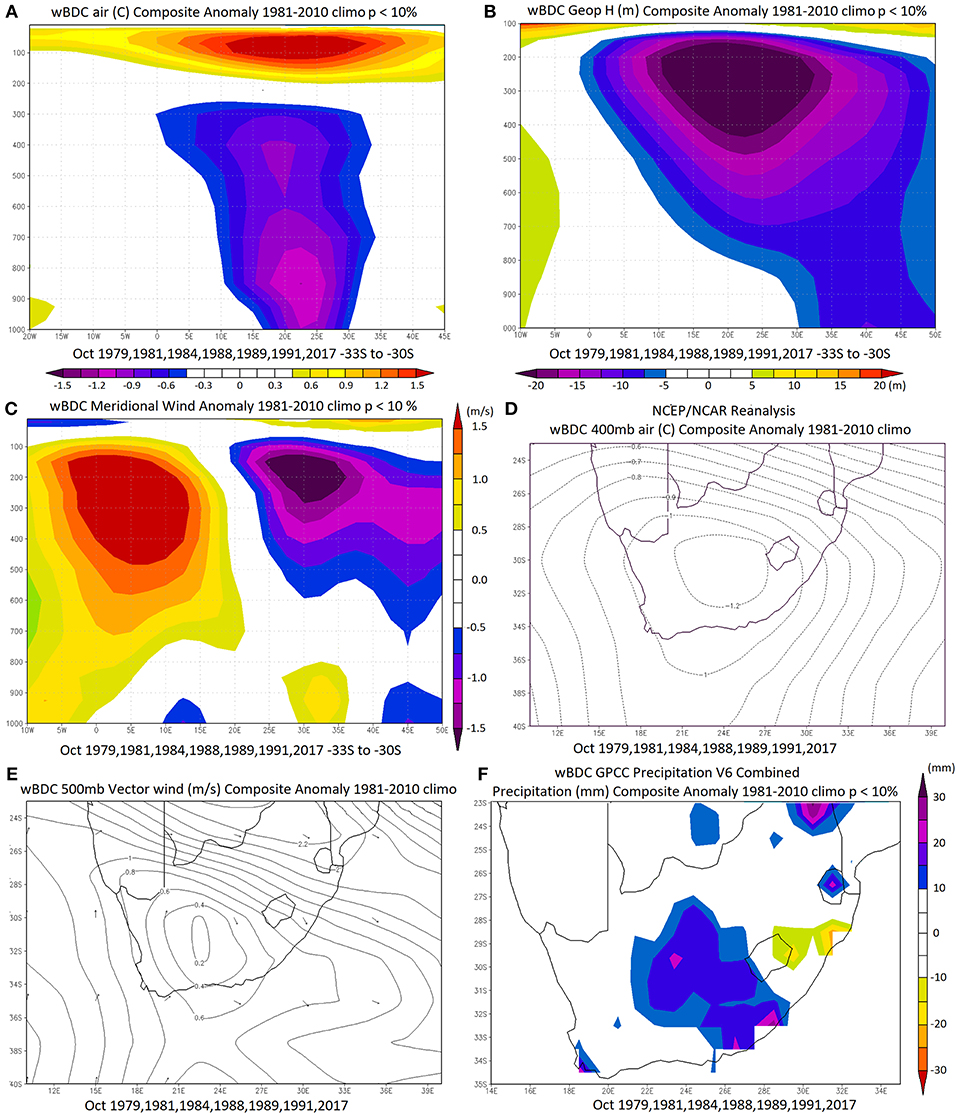
Figure 6. Vertical slice of the (A) air temperature (°C), (B) geopotential height (m) and (C) the meridional wind (m/s) pattern for the wBDC composite anomalies averaged over (A) 21°E to 25°E and extending from 40°S to 20°N, (B) 33°S to 30°S and covering 10°W to 45°E. Composites but for (D) air temperature anomalies (°C) for the 400 mb level, (E) same as for (D) but for the 500 mb wind (m/s) level and (F) land only rainfall anomalies (mm) with the region covered indicated in each panel. The anomalies are with respect to the 1981–2010 climatology. Shaded regions are significant above the 90% confidence level. Years for the composites are indicated in the insert.
Although we did not display corresponding figures for the sBDC, the effect is more or less the opposite. In fact the TOC is strongly correlated to the tropopause height (Steinbrecht et al., 1998) which is inversely related to the tropospheric geopotential height with w(s)BDC events corresponding to high (low) TOC. In this regard, the elevated tropospheric geopotential height has a maximum response at the upper part coinciding with the LSO deficit and tropospheric warming. This leads to an anomalous anticylonic circulation, a mechanism with considerable suppression of cloud development resulting in the observed significant negative rainfall anomalies. These, as opposed to the wBDC composites, are not largely restricted to the central region but spreads from most of central to eastern regions of South Africa. In the same vein, the compression of the tropospheric column in response to the LST cooling shown in Figures 5C,D favors the development of high pressure anomalies from the upper to middle troposphere which promotes blocking signatures over South Africa. It is most likely that this may limit the development of the late spring early summer diagonal cloudbands that normally form over southern Angola (Harrison, 1984; Hart et al., 2013) from extending to reach central and eastern South Africa hence resulting in the observed significant rainfall deficits over most of the subregion. However, as the LSO anomalies abruptly disappear in November, so does the anomalous circulation patterns together with the associated rainfall anomalies. Hence although the diagonal cloud bands are a summer phenomenon, their development is essentially impacted on by the LSO modulation during the month of October. But since October marks the beginning of the summer rainfall season, these rainfall anomalies, though significant for this month have magnitudes which appear not to have a strong bearing on the overall outcome of the rainfall season. In this way we have identified anomalous features in the tropospheric general circulation and climate over South Africa that can be traced back to anomalies in the October LSO field above.
Discussions and Conclusions
Our results are quite novel. While it is conventional knowledge that SATmax increases over South Africa has been extensively related to the increase in GHGs (e.g., James and Washington, 2013), that due to the LSO depletion has so far not been considered. Unlike GHG impacts which are expected to be rather unrestricted spatially (affecting all regions) and temporarily (all months and years), stratospheric ozone forcing, despite having seasonal dependence that is characterized by a shift, also has a strong geographical dependence related to the wBDC and sBDC impacts on surface temperature and precipitation. The wBDC composites are related to significantly negative and positive surface temperature and precipitation anomalies respectively, while the reverse is true for the sBDC events. Because of the global warming-induced strengthening of the BDC, the resulting increased frequency of sBDC may result in substantial ozone depletion over South Africa in the coming decades in particular winters and springs. In this context, the ozone over South Africa will steadily decrease with the projected global warming rather than increase due to the global ozone recovery that is attributed to the implementation of MP and its amendments. This should elevate SATmax whilst drying the region hence inducing alterations in the regional climate which is not necessarily directly linked to GHG induced climate change. As such we would then expect an improvement in the representativeness of tropospheric and surface temperature when observed ozone data is assimilated in the climatological forecast models for the spring period. On the other hand, the sBDC events, which are bound to increase in the warming climate should have implications for regional UVB radiation changes, notably enhancing the clear-sky UVB radiation levels over the South African continent during spring. This is because of the expected increased sBDC events which facilitate middle level anticyclonic circulation. These findings, especially that they are on populated regions of the SH, may not only have implications for weather and seasonal forecasting including future climate change, but may inform on spring UVB impacts on the health of society, agriculture and ecosystems.
In any case the statistical methods applied in this work may not conclusively prove the cause-effect behavior between the LSO and SATmax/rainfall but provides a basic way of connecting the BDC forced lower stratospheric spring ozone variability to South Africa's climate. As such it can be considered an initial step toward identifying the physical mechanism that underlies the causal link. The proposed feedback mechanisms between LSO and surface temperature warrants further investigation beyond this publication, as our analysis clearly shows changes of ozone in the lower stratosphere down to the troposphere and surface temperatures being related to what appears to be radiative forcing-like response. However, it has to be noted that our observational results are consistent with most modeling studies which were able to successfully link the LSO variability with surface response (e.g., Gillett et al., 2009; Waugh et al., 2009). This was achieved through specifying non-zonal ozone forcing using ozone anomaly amplitudes within the observed range of the last three decades.
Author Contributions
DM conceptualized the concept of the manuscript including the analysis and writing. GM did the analysis and reviewing of the manuscript.
Funding
The first author is supported by Bindura University of Science. The Afromontane Research Unit (ARU) and Geography Department of the Free State University provided additional research support facilities.
Conflict of Interest Statement
The authors declare that the research was conducted in the absence of any commercial or financial relationships that could be construed as a potential conflict of interest.
References
Abalos, M., Ploeger, F., Konopka, P., Randel, W. J., and Serrano, E. (2013). Ozone seasonality above the tropical tropopause: reconciling the Eulerian and Lagrangian perspectives of transport processes. Atmos. Chem. Phys. 13, 10787–10794, doi: 10.5194/acp-13-10787-2013
Abalos, M., Randel, W. J., and Serrano, E. (2012). Variability in upwelling across the tropical tropopause and correlations with tracers in the lower stratosphere. Atmos. Chem. Phys. 12, 11505–11517. doi: 10.5194/acp-12-11505-2012
Abalos, M., Randel, W. J., and Serrano, E. (2014). Dynamical forcing of subseasonal variability in the tropical brewer–dobson circulation. J. Atmos. Sci. 71, 3439–3453. doi: 10.1175/JAS-D-13-0366.1
Ball, W. T., Alsing, J., Mortlock, D. J., Staehelin, J., Haigh, J. D., Peter, T., et al. (2018). Evidence for a continuous decline in lower stratospheric ozone offsetting ozone layer recovery. Atmos. Chem. Phys. 18, 1379–1394, doi: 10.5194/acp-18-1379-2018
Ball, W. T., Kuchař, A., Rozanov, E. V., Staehelin, J., Tummon, F., Smith, A. K., et al. (2016). An upper-branch Brewer-Dobson circulation index for attribution of stratospheric variability and improved ozone and temperature trend analysis. Atmos. Chem. Phys. 16, 15485–15500. doi: 10.5194/acp-2016-449
Barodka, S., Krasouski, A., Mitskevich, Y., and Shalamyansky, A. (2015). “Influence of stratospheric ozone distribution on tropospheric circulation patterns,” in Geophysical Research Abstracts EGU General Assembly (Vienna).
Behera, S. K., Luo, J.-J., Masson, S., Delecluse, P., Gualdi, S., Navarra, A., et al. (2005). Paramount impact of the Indian Ocean Dipole on the East African short rains: A CGCM study. J. Clim. 18, 4514–4530. doi: 10.1175/JCLI3541.1
Bencherif, H., El Amraoui, L., Kirgis, G., Leclair De Bellevue, J., Hauchecorne, A., Mzé, N., et al. (2011). Analysis of a rapid increase of stratospheric ozone during late austral summer 2008 over Kerguelen (49.4° S, 70.3° E). Atmos. Chem. Phys. 11, 363–373. doi: 10.5194/acp-11-363-2011
Bencherif, H., El-Amraoui, L., Semane, N., Massart, S., Charyulu, D. V., Hauchecorne, A., et al. (2007). Examination of the 2002 major warming in the Southern Hemisphere using ground-based and Odin/SMR assimilated data: stratospheric ozone distributions and tropic/mid-latitude exchange. Can. J. Phys. 85, 1287–1300. doi: 10.1139/p07-143
Birner, T., and Bönisch, H. (2011). Residual circulation trajectories and transit times into the extratropical lowermost stratosphere. Atmos. Chem. Phys. 11, 817–827. doi: 10.5194/acp-11-817-2011
Bönisch, H., Engel, A., Birner, T., Hoor, P., Tarasick, D. W., and Ray, E. A. (2011). On the structural changes in the Brewer-Dobson circulation after 2000. Atmos. Chem. Phys. 11, 3937–3948. doi: 10.5194/acp-11-3937-2011
Breaker, L. C. (2007). A closer look at regime shifts based on coastal observations along the eastern boundary of the North Pacific. Continental Shelf Res. 27 2250–2277. doi: 10.1016/j.csr.2007.05.018
Brunner, D., Staehelin, J., Maeder, J. A., Wohltmann, I., and Bodeker, G. E. (2006). Variability and trends in total and vertically resolved stratospheric ozone based on the CATO ozone data set. Atmos. Chem. Phys. 6, 4985–5008, doi: 10.5194/acp-6-4985-2006.
Butchart, N. (2014). The Brewer-Dobson circulation, Rev. Geophys., 52, 157–184, doi: 10.1002/2013RG000448
Calvo, N., Garcia, R. R., Randel, W. J., and Marsh, D. (2010). Dynamical mechanism for the increase in tropical upwelling in the lowermost tropical stratosphere during warm ENSO events. J. Atmos. Sci. 67, 2331–2340. doi: 10.1175/2010JAS3433.1
Chandra, S., Varotsos, C., and Flynn, L. E. (1996). The mid-latitude total ozone trends in the northern hemisphere. Geophys. Res. Lett. 23, 555–558.
Eckert, E., von Clarmann, T., Kiefer, M., Stiller, G. P., Lossow, S., Glatthor, N., et al. (2014). Drift-corrected trends and periodic variations in MIPAS IMK/IAA ozone measurements. Atmos. Chem. Phys. 14, 2571–2589. doi: 10.5194/acp-14-2571-2014
Egorova, T., Rozanov, E., Gröbner, J., Hauser, M., and Schmutz, W. (2013). Montreal protocol benefits simulated with CCMSOCOL. Atmos. Chem. Phys. 13, 3811–3823. doi: 10.5194/acp-13-3811-2013
El Amraoui, L., Attié, J.-L., Semane, N., Claeyman, M., Peuch, V. H., Warner, J., et al. (2010). Midlatitude stratosphere – troposphere exchange as diagnosed by MLS O3 and MOPITT CO assimilated fields. Atmos. Chem. Phys. 10, 2175–2194. doi: 10.5194/acp-10-2175-2010
Eyring, V., Waugh, D. W., Bodeker, G. E., Cordero, E., Akiyoshi, H., Austin, J., et al. (2007). Multimodel projections of stratospheric ozone in the 21st century. J. Geophys. Res. 112, D16303. doi: 10.1029/2006JD008332
Flury, T., Wu, D. L., and Read, W. G. (2013). Variability in the speed of the Brewer–Dobson circulation as observed by Aura/MLS. Atmos. Chem. Phys. 13, 4563–4575. doi: 10.5194/acp-13-4563-2013
Forster, P. M., and Shine, K. P. (1997). Radiative forcing and temperature trends from stratospheric ozone changes. J. Geophys. Res. 102, 10841–10855. doi: 10.1029/96JD03510
Garcia, R. R., and Randel, W. J. (2008). Acceleration of the Brewer–Dobson circulation due to increases in greenhouse gases. J. Atmos. Sci. 65, 2731–2739. doi: 10.1175/2008JAS2712.1
Gerber, E. P. (2012). Stratospheric versus tropospheric control of the strength and structure of the Brewer-Dobson circulation. J. Atmos. Sci. 69, 2857–2877. doi: 10.1175/JAS-D-11-0341.1
Gettelman, A., Hegglin, M. I., Kim, J., Fujiwara, M., Birner, T., Kremser, S., et al. (2010). Multimodel assessment of the upper troposphere and lower stratosphere: tropics and global trends. J. Geophys. Res. 115:D00M08. doi: 10.1029/2009JD013638
Gettelman, A., Hoor, P., Pan, L. L., Randel, W. J., Hegglin, M. I., and Birner, T. (2011). The extratropical upper troposphere and lower stratosphere. Rev. Geophys. 49:RG3003. doi: 10.1029/2011RG000355
Gillett, N. P., Scinocca, J. F., Plummer, D. A., and Reader, M. C. (2009). Sensitivity of climate to dynamically-consistent zonal asymmetries in ozone, Geophys. Res. Lett. 36:L10809. doi: 10.1029/2009GL037246
Graf, R., and Tomczyk, A. M. (2018). The impact of cumulative negative air temperature degree-days on the appearance of ice cover on a river in relation to atmospheric circulation. Atmosphere 9:204. doi: 10.3390/atmos9060204
Grise, K. M., and Thompson, D. W. J. (2013). On the signatures of equatorial and extratropical wave forcing in tropical tropopause layer temperatures. J. Atmos. Sci. 70, 1084–1102. doi: 10.1175/JAS-D-12-0163.1
Hadjinicolaou, P., and Pyle, J. A. (2004). The impact of arctic ozone depletion on northern middle latitudes: interannual variability and dynamical control. J. Atmos. Chem. 47, 25–43. doi: 10.1023/B:JOCH.0000012242.06578.6c
Harris, N. R. P., Hassler, B., Tummon, F., Bodeker, G. E., Hubert, D., Petropavlovskikh, I., et al. (2015). Past changes in the vertical distribution of ozone—Part 3: Analysis and interpretation of trends. Atmos. Chem. Phys. 15, 9965–9982. doi: 10.5194/acp-15-9965-2015
Harrison, M. S. J. (1984). A generalized classification of South African rain-bearing synoptic systems. J. Climatol. 4, 547–560. doi: 10.1002/joc.3370040510
Hart, N. C. G., Reason, C. J. C., and Fauchereau, N. (2013): Cloud bands over southern Africa: Seasonality contribution to rainfall variability modulation by the MJO. Climate Dyn. 41, 1199–1212. doi: 10.1007/s00382-012-1589-4
Heim, N., Fisher, J. T., Clevenger, A., Paczkowski, J., and Volpe, J. (2017). Cumulative effects of climate and landscape change drive spatial distribution of Rocky Mountain wolverine (Gulo gulo L.) Ecol. Evol. 7, 8903–8914. doi: 10.1002/ece3.3337
Holton, J. R., Haynes, P. H., McIntyre, M. E., Douglass, A. R., Rood, R. B., and Pfister, L. (1995). Stratosphere–troposphere exchange. Rev. Geophys. 33. 403–439, doi: 10.1029/95RG02097
Hood, L. L., McCormack, J. P., and Labitzke, K. (1997). An investigation ofdynamical contributions to midlatitude ozone trends in winter. J. Geophys. Res. 102, 13079–13093.
Hood, L. L., and Soukharev, B. E. (2005). Interannual variations of total ozone at northern midlatitudes correlated with EP flux and potential vorticity. J. Atmos. Sci. 62, 3724–3740. doi: 10.1175/JAS3559.1
James, R., and Washington, R. (2013). Changes in African temperature and precipitation associated with degrees of global warming. Climat. Change 117:859. doi: 10.1007/s10584-012-0581-7
Kalnay, E., Kanamitsu, M., Kistler, R., Collins, W., Deaven, D., Gandin, L., et al. (1996). The NCEP/NCAR 40-year reanalysis project. Bull. Am. Meteorol. Soc. 77, 437–471.
Kirgis, G., Leblanc, T., McDermid, I. S., and Walsh, T. D. (2013). Stratospheric ozone interannual variability (1995–2011) as observed by lidar and satellite at Mauna Loa Observatory, HI and Table Mountain Facility, CA. Atmos. Chem. Phys. 13, 5033–5047. doi: 10.5194/acp-13-5033-2013
Kirk-Davidoff, D. B., Hintsa, E. J., Anderson, J. G., and Keith, D. W. (1999). The effect of climate change on ozone depletion through changes in stratospheric water vapour. Nature 402, 399–401. doi: 10.1038/46521
Konopka, P., Groo,ß, J.-U., Günther, G., Ploeger, F., Pommrich, R., Müller, R., and Livesey, N. (2010), Annual cycle of ozone at above the tropical tropopause: Observations versus simulations with the Chemical Lagrangian Model of the Stratosphere (CLaMS). Atmos. Chem. Phys. 10, 121–132. doi: 10.5194/acp-10-121-2010
Konopka, P., Ploeger, F., Tao, M., Birner, T., and Riese, M. (2015), Hemispheric asymmetries seasonality of mean age of air in the lower stratosphere: Deep versus shallow branch of the Brewer-Dobson circulation. J. Geophys. Res. Atmos. 120, 2053–2066. doi: 10.1002/2014JD022429
Li, F., Stolarski, R. S., and Newman, P. A. (2009). Stratospheric ozone in the post-CFC era. Atmos. Chem. Phys. 9, 2207–2213. doi: 10.5194/acp-9-2207-2009
Manatsa, D., Matarira, C. H., Mushore, T. D., and Mudavanhu, C. (2015). Southern Africa winter temperature shifts and their link to the Southern Annular Mode. J. Climate Dyna. 45, 2337–2350. doi: 10.1007/s00382-015-2474-8
Manatsa, D., Morioka, Y., Behera, S. K., Yamagata, T., and Matarira, C. H. (2013). Link between Antarctic ozone depletion and summer warming over southern Africa. Nat. Geosci. 6, 934–939. doi: 10.1038/ngeo1968
Manatsa, D., and Mukwada, G. (2017). A connection from stratospheric ozone to El Niño-Southern Oscillation. Nat. Sci. Rep. 7:5558. doi: 10.1038/s41598-017-05111-8
Marshall, G. J. (2003). Trends in the Southern Annular Mode from observations and reanalyses. J. Clim. 16, 4134–4143. doi: 10.1175/1520-0442(2003)
McPeters, R. D., Krueger, A. J., Bhartia, P. K., Herman, J. R., Wellemeyer, C. G., Seftor, C. J., et al. (1998). Earth Probe Total Ozone Mapping Spectrometer (TOMS) Data Products User's Guide, Washington, DC: NASA.
Moalafhi, D. B., Ashish, S., and Evans, J. P. (2017). Reconstructing hydro-climatological data using dynamical downscaling of reanalysis products in data-sparse regions, application to the Limpopo catchment in southern Africa J. Hydrol. 12, 378–395. doi: 10.1016/j.ejrh.2017.07.001
Molina, L. T., and Molina, M. J. (1987). Production of Cl2O2 from the self-reaction of the ClO radical. J. Phys. Chem. 91, 433–436.
Muller, R. A., Rohde, R., Jacobsen, R., Muller, E., and Wickham, C. (2013). A new estimate of the average earth surface land temperature spanning 1753–2011. Geoinfor. Geostat. Overv. 1, 1–7. doi: 10.4172/2327-4581.1000101
Nath, O., and Sridharan, S. (2015). Equatorial middle atmospheric chemical composition changes during sudden stratospheric warming events, Atmos. Chem. Phys. Discuss. 15, 23969–23988. doi: 10.5194/acpd-15-23969-2015
Newchurch, M. J., Yang, E. S., Cunnold, D. M., Reinsel, G. C., Zawodny, J. M., Russel, I. I. I., et al. (2003). Evidence for slowdown in stratospheric ozone loss: first stage of ozone recovery. J. Geophys. Res. 108:4507. doi: 10.1029/2003JD003471
North, G. R., Bell, T. L., Cahalan, R. F., and Mohen, F. J. (1982). Sampling errors in the estimation of empirical orthogonal functions. Mon. Wea. Rev. 110, 699–706. doi: 10.1175/1520-0493(1982)110,0699:SEITEO.2.0.CO;2
Olsen, M. A., Schoeberl, M. R., and Nielsen, J. E. (2007). Response of stratospheric circulation and stratosphere–troposphere exchange to changing sea surface temperatures. J. Geophys. Res. 112:D16104. doi: 10.1029/2006JD008012
Partanen, A., Martin, L., and Damon, M. H. (2017). Seasonal climate change patterns due to cumulative CO2emissions. Environ. Res. Lett. 12:7. doi: 10.1088/1748-9326/aa6eb0
Polvani, L. M., Wang, L., Aquila, V., and Waugh, D. W. (2017). The impact of ozone-depleting substances on tropical upwelling, as revealed by the absence of lower-stratospheric cooling since the late 1990s. J. Clim. 30, 2523–2534. doi: 10.1175/JCLI-D-16-0532.1
Previdi, M., and Polvani, L. M. (2014). Climate system response to stratospheric ozone depletion and recovery. Q. J. Roy. Meteor. Soc. 140, 2401–2419. doi: 10.1002/qj.2330
Randel, W. J., Garcia, R. R., Calvo, N., and Marsh, D. (2009). ENSO influence on zonal mean temperature and ozone in the tropical lower stratosphere, J. Geophys. Res. 36:L15822. doi: 10.1029/2009GL039343
Randel, W. J., Park, M., Wu, F., and Livesey, N. (2007). A large annual cycle in ozone above the tropical tropopause linked to the Brewer–Dobson circulation. J. Atmos. Sci. 64, 4479–4488. doi: 10.1175/2007JAS2409.1
Randel, W. J., Polvani, L., Wu, F., Kinnison, D. E., Zou, C.-Z., and Mears, C. (2017). Troposphere-stratosphere temperature trends derived from satellite data compared with ensemble simulations from WACCM. J. Geophys. Res. 122, 9651–9667. doi: 10.1002/2017JD027158
Randel, W. J., and Thompson, A. M. (2011). Interannual variability and trends in tropical ozone derived from SAGE II satellite data and SHADOZ ozonesondes. J. Geophys. Res. Atmos. 116:D07303. doi: 10.1029/2010jd015195
Randel, W. J., Wu, F., and Stolarski, R. (2002). Changes in Column Ozone Correlated with the Stratospheric EP Flux. J. Meteorol. Soc. Japan 80, 849–862. doi: 10.2151/jmsj.80.849
Rodionov, S., and Overland, J. E. (2005). Application of a sequential regime shift detection method to the Bering Sea ecosystem. e ICES J. Marine Sci. 62, 328–332. doi: 10.1016/j.icesjms.2005.01.013
Salby, M. (2008). Involvement of the Brewer-Dobson circulation in changes of stratospheric temperature and ozone. Dyn. Atmos. Oceans 44, 143–164. doi: 10.1016/j.dynatmoce.2006.11.002
Sharma, R. (2001). Impact of solar UV-B on tropical ecosystems and agriculture. case study: effect of UV-B on rice. Proc. SEAWIT98 SEAWPIT2000 1, 92–101.
Shepherd, T. G. (2007). Transport in the middle atmosphere. J. Meteor. Soc. Japan 85, 165–191. doi: 10.2151/jmsj.85B.165
Shepherd, T. G., and McLandress, C. (2011). A robust mechanism for strengthening of the Brewer–Dobson circulation in response to climate change: critical-layer control of subtropical wave breaking. J. Atmos. Sci. 68, 784–797. doi: 10.1175/2010JAS3608.1
Sioris, C. E., McLinden, C. A., Fioletov, V. E., Adams, C., Zawodny, J. M., Bourassa, A. E., et al. (2014). Trend and variability in ozone in the tropical lower stratosphere over 2.5 solar cycles observed by SAGE II and OSIRIS, Atmos. Chem. Phys. 14, 3479–3496. doi: 10.5194/acp-14-3479-2014
Sivakumar, V., and Ogunniyi, J. (2017). Ozone climatology and variability over Irene, South Africa determined by ground based and satellite observations. part 1: vertical variations in the troposphere and stratosphere. Atmósfera 30, 337–353. doi: 10.20937/ATM.2017.30.04.05
Solomon, S., Garcia, R. R., Rowland, F. S., and Wuebbles, D. J. (1986). On the depletion of Antarctic ozone. Nature 321. 755–758.
Solomon, S., Ivy, D. J., Kinnison, D., Mills, M. J., Neely, I. I. I. R. R., Schmidt, A., et al. (2016), Emergence of healing in the Antarctic ozone layer. Science 252, 269–274. doi: 10.1126/science.aae0061
Steinbrecht, W., Claude, H., and Kohler, U. (1998). Correlations between tropopause height and total ozone: Implications for long-term changes. J. Geophys. Res. 103, 19183–19192.
Steinbrecht, W., Claude, H., Schonenborn, F., McDermid, I. S., Leblanc, T., Godin-Beekmann, S., et al. (2009). Ozone and temperature trends in the upper stratosphere at five stations of the network for the detection of atmospheric composition change. Int. J. Remote Sens. 30, 3875–3886. doi: 10.1080/01431160902821841
Thompson, A. M., Diab, R. D., Bodeker, G. E., Zunckel, M., Coetzee, G. J. R., Archer, C. B., et al. (1996). Ozone over southern Africa during SAFARI-92/TRACE A. J. Geophys. Res. Atmos. 101, 23793–23807. doi: 10.1029/95jd02459
Trenberth, K. E., Fasullo, J. T., and Balmaseda, M. A. (2014). Earth's energy imbalance. J. Clim. 27, 3129–3144. doi: 10.1175/JCLI-D-13-00294.1
Ueyama, R., Gerber, E. P., Wallace, J. M., and Frierson, D. M. W. (2013). The role of high-latitude waves in the intraseasonal to seasonal variability of tropical upwelling in the Brewer–Dobson circulation. J. Atmos. Sci. 70, 1631–1648. doi: 10.1175/JAS-D-12-0174.1
Ueyama, R., and Wallace, J. M. (2010). To what extent does high-latitude wave forcing drive tropical upwelling in the brewer–dobson circulation? J. Atmos. Sci. 67, 1232–1246. doi: 10.1175/2009JAS3216.1
UNEP United Nations Environment Programme (1999). 1998 Assessment Report of the Halons Technical Options Committee, Nairobi, 286
van der, A. R. J., Allaart, M. A. F., and Eskes, H. J. (2015). Extended and refined multi sensor reanalysis of total ozone for the period 1970–2012, Atmos. Meas. Tech. 8, 3021–3035. doi: 10.5194/amt-8-3021-2015
Ward, P. L. (2016). Ozone depletion explains global warming. Curr. Phys. Chem. 6:4. doi: 10.2174/1877946806999160629080145
Waugh, D. W., Oman, L., Newman, P. A., Stolarski, R. S., Pawson, S., Nielsen, J. E., et al. (2009). Effect of zonal asymmetries in stratospheric ozone on simulated Southern Hemisphere climate trends. Geophys. Res. Lett. 36:L18701. doi: 10.1029/2009GL040419
Waugh, D. W., and Polvani, L. M. (2000). Climatology of intrusions into the tropical upper troposphere. Geophys. Res. Lett. 27, 3857–3860. doi: 10.1029/2000GL012250
Weber, M., Dhomse, S., Wittrock, F., Richter, A., Sinnhuber, B.-M., and Burrows, J. P. (2003). Dynamical control of NH and SH winter/spring total ozone from GOME observations in 1995-2002. Geophys. Res. Lett. 30:1853. doi: 10.1029/2002G.L.016799
Wetherill, G. B., and Brown, D. W. (1991). Statistical Process Control: Theory and Practice. London: Chapman and Hall.
WMO Scientific Assessment of Ozone Depletion (2014). Global Ozone Research and Project Report, World Meteorological Organization. Geneva. 416.
Wohltmann, I., Lehmann, R., Rex, M., Brunner, D., and Mäder, J. A. (2007). A process-oriented regression model for column ozone. J. Geophys. Res. Atmos. 112:D12304. doi: 10.1029/2006JD007573
Yang, G.-Y., and Slingo, J. (2001). The diurnal cycle in the Tropics. Mon. Weather Rev. 129, 784–801. doi: 10.1175/1520-0493(2001)129<0784:TDCITT>2.0.CO;2
Young, P. J., Butler, A. H., Calvo, N., Haimberger, L., Kushner, P. J., Marsh, D. R., et al. (2013). Agreement in late twentieth century Southern Hemisphere stratospheric temperature trends in observations and CCMVal-2, CMIP3, and CMIP5 models. J. Geophys. Res. Atmos. 118:605–613. doi: 10.1002/jgrd.50126
Young, P. J., Thompson, D. W. J., Rosenlof, K. H., Solomon, S., and Lamarque, J.-F. (2011), The seasonal cycle interannual variability in stratospheric temperatures links to the Brewer-Dobson circulation: an analysis of MSU SSU data. J. Clim. 24, 6243–6258. doi: 10.1175/JCLI-D-10-05028.1
Yulaeva, E., Holton, J. R., and Wallace, J. M. (1994). On the cause of the annual cycle in tropical lower-stratospheric temperature. J. Atmos. Sci. 51, 169–174. doi: 10.1175/1520-0469(1994)051<0169:OTCOTA>2.0.CO;2
Keywords: Brewer Dobson Circulation, tropical and subtropical lower stratosphere, ultra violet radiation, maximum surface temperature and rainfall, South Africa
Citation: Manatsa D and Mukwada G (2019) Spring Ozone's Connection to South Africa's Temperature and Rainfall. Front. Earth Sci. 7:27. doi: 10.3389/feart.2019.00027
Received: 17 October 2018; Accepted: 05 February 2019;
Published: 26 February 2019.
Edited by:
Alexandre M. Ramos, Universidade de Lisboa, PortugalReviewed by:
Ross Campbell Blamey, University of Cape Town, South AfricaAna Cristina Russo, Universidade de Lisboa, Portugal
Copyright © 2019 Manatsa and Mukwada. This is an open-access article distributed under the terms of the Creative Commons Attribution License (CC BY). The use, distribution or reproduction in other forums is permitted, provided the original author(s) and the copyright owner(s) are credited and that the original publication in this journal is cited, in accordance with accepted academic practice. No use, distribution or reproduction is permitted which does not comply with these terms.
*Correspondence: Desmond Manatsa, ZG1hbmF0c2FAZ21haWwuY29t