Soda Bottle Science—Citizen Science Monsoon Precipitation Monitoring in Nepal

Introduction

Precipitation is the main terrestrial input of the global water cycle; without it, our springs, streams, lakes, and communities would gradually disappear. Understanding the spatial and temporal distribution of precipitation is therefore critical for characterizing water and energy balances, water resources planning, irrigation management, flood forecasting, and several other resource management and planning activities (Lettenmaier et al., 2017). However, observing, and moreover understanding, precipitation variability over space and time is fraught with difficulty and uncertainty. Because of these challenges, there are persistent, but spatially heterogeneous, precipitation data gaps that need to be addressed (Kidd et al., 2017).

Accuracy is a primary concern, even for common precipitation measurement methods (Krajewski et al., 2003; Villarini et al., 2008) including: manual and automatic gauges, radar, and satellite remote sensing. Manual and automatic gauges are expensive to maintain and thus generally do not lead to adequate spatial representations of precipitation (e.g., Volkmann et al., 2010). For example, the total area of all the rain gauges in the world is less than half a football field (Kidd et al., 2017), or 0.000000002% of the global terrestrial landscape. Precipitation radars can provide meaningful data between gauges, but are subject to errors from beam blockage, range effects, and imperfect relationships between rainfall and backscatter (Kidd et al., 2017). Additionally, radars are expensive and operate by line of sight, so spatial cover of radar in mountainous terrains like Nepal can be limited. Satellite remotely sensed precipitation products have the benefit of global coverage, but can be impacted by random errors and bias (e.g., Koutsouris et al., 2016) arising from the indirect linkage between the observed parameters and precipitation and imperfect algorithms (Sun et al., 2018). Clearly, there remain precipitation data gaps and uncertainties that need to be filled.

Low-cost sensors and consumer electronics can play a role in closing these data gaps (Hut, 2013; Tauro et al., 2018). In general, the potential of low-cost sensors to improve understanding of a process depends on the interplay between (1) the spatial heterogeneity of the process being observed, (2) the impacts on accuracy of the low-cost sensor, and (3) the observational cost savings. The need for higher density observations increases as the spatial heterogeneity of the process being observed increases. So, if (1) the observed process has high spatial heterogeneity, and (2) the low-cost sensor provides high accuracy, with (3) high cost savings, the potential of the low-cost sensor to improve understanding of the process is considered high.

Citizen science has emerged as a promising tool to help fill data gaps. At the same time, citizen science can improve overall scientific literacy and reconnect people with their natural resources. McKinley et al. (2017) define citizen science as “the practice of engaging the public in a scientific project.” They go on to clarify that crowdsourcing is another way for public participation in science through “… large numbers of people processing and analyzing data.” Notable examples of citizen science precipitation monitoring include: the Community Collaborative Rain, Hail, and Snow Network (CoCoRaHS: www.cocorahs.org); Weather Underground (www.wunderground.com); Met Office Weather Observation Website (WOW: wow.metoffice.gov.uk/); UK Citizen Rainfall Network (Illingworth et al., 2014); the NOAA Citizen Weather Observer Program (CWOP: wxqa.com); and an internet-connected amateur weather station network called Netatmo (www.netatmo.com) (Kidd et al., 2017).

Launched in the spring of 1998 by the Colorado Climate Center at Colorado State University, CoCoRaHS is a volunteer-led precipitation monitoring effort (Reges et al., 2016). Volunteers measure daily precipitation with a standardized 102 mm (4-inch) gauge (Sevruk and Klemm, 1989) and report their data via an online system. While CoCoRaHS was established in response to small scale flash floods, it has grown into the world's largest volunteer precipitation monitoring network, with over 20,000 active observers in the United States, Canada, the U.S. Virgin Islands, the Bahamas, and Puerto Rico (Cifelli et al., 2005).

In Nepal, three specific attempts have been made to launch citizen science precipitation measurement campaigns. The first was a single year effort in 1998 initiated by Nepali scientists Ajaya Dixit and Dipak Gyawali who partnered with community members to measure rainfall in the Rohini River watershed, a tributary to the Ganges, in south-central Nepal. The second was launched by Recham Consulting in 2003, and included 17 gauges similar to US National Weather Service 203 mm (8-inch) gauges in the Kathmandu Valley. However, the project stalled after only a few years of data collection. The third, Community Based Rainfall Measurement Nepal (CORAM-Nepal), was launched in 2015 with seven high schools in the Kathmandu Valley (Pokharel et al., 2016). CORAM's approach to obtain rainfall data is to partner with local high school science teachers and students, but other community members were also welcome to participate. CORAM-Nepal uses standard 102 mm (4-inch) CoCoRaHS gauges and collects data from schools monthly by phone call or site visits. All of these previous efforts grappled with the challenges of sustainable (1) funding, (2) human resources, and (3) technological issues related to data collection, quality control, data storage, analysis, and dissemination of precipitation data.

What is needed is a sustained effort to monitor precipitation via citizen scientists. To achieve sustainability, such an effort needs to be both accurate and cost effective. The latter part may be attainable through leveraging low-tech MacGyver-type solutions—but only if they lead to accurate and reproducible observations (note that MacGyver was a popular television show in the late 1980s and early 1990s that often highlighted the ability of the protagonist—Angus “Mac” MacGyver—to make just about anything from commonly available materials). To this end, our research was conducted in the context of SmartPhones4Water (S4W), a California based non-profit organization investigating how young researchers, citizen scientists, and mobile technology can be mobilized to help close growing water data gaps (including precipitation). S4W's first pilot project in Nepal (S4W-Nepal; Davids et al., 2018a,b) was launched in early 2017. This paper focuses on the 2018 monsoon (May through September) precipitation monitoring efforts in Nepal using low-tech gauges (in contrast to high-tech approaches like Netatmo).

Our research questions can be organized into two primary categories: (1) low-cost S4W precipitation gauge analyses and (2) citizen scientist involvement.

1. S4W precipitation gauge analyses

a. What are the types and magnitudes of errors for S4W's low-cost precipitation gauges?

b. How do precipitation measurements from S4W's low-cost gauges compare to other commonly used gauges, including the Department of Hydrology and Meteorology (DHM), Nepal standard gauge?

2. Citizen scientist involvement

a. How effective were our methods to recruit citizens to join the monsoon precipitation monitoring campaign?

b. How effective were our methods to motivate citizens to continue taking daily precipitation measurements?

c. What were the types and frequencies of common citizen scientist observation errors?

d. What were the average costs per observation for citizen scientists, and did this relate to citizen scientist performance?

Context and Study Area

To answer our research questions, S4W-Nepal launched a 2018 monsoon precipitation monitoring campaign; 154 citizen scientists generated 6,656 precipitation measurements using low-cost (<1 USD) S4W gauges constructed from repurposed soda bottles, concrete, and rulers. Measurements were recorded with smartphones using an Android-based application called Open Data Kit (ODK) Collect, and included GPS-generated coordinates, observation date and time, photographs, and citizen scientist reported readings. Measurements were primarily in the Kathmandu Valley and Kaski District of Nepal (Figure 1).

FIGURE 1

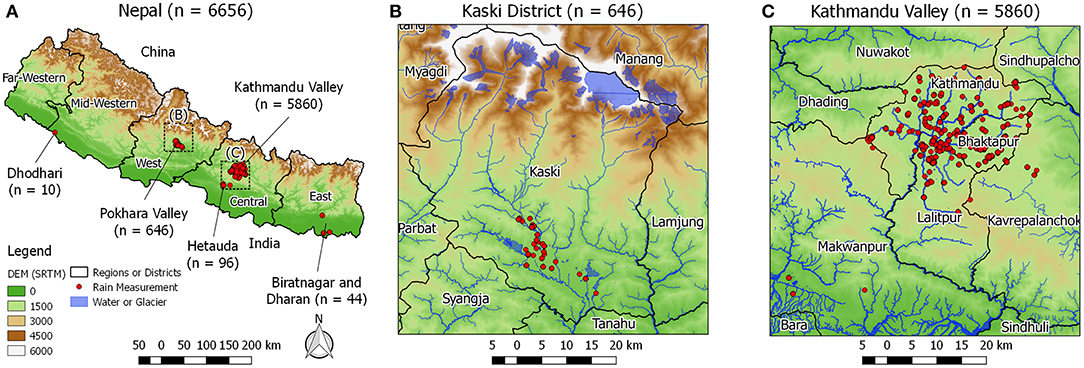
Figure 1. Locations of 2018 Monsoon (May to September) precipitation measurements with the number of measurements shown in parentheses for (A) Nepal, with enlarged views of (B) the Kaski District, including the Pokhara Valley, and (C) the Kathmandu Valley. Topography shown from a Shuttle Radar Telemetry Mission (SRTM) 90-m digital elevation model (DEM) (SRTM, 2000).

Precipitation in Nepal is highly heterogeneous, both spatially and temporally. Spatial variability of precipitation in Nepal is driven by (1) strong convection and (2) orographic effects (Nayava, 1980). Temporal fluctuations are mostly due to the South Asian summer monsoon (June to September)—a south to north moisture movement perpendicular to the Himalayas (Figure 1) along the southern rim of the Tibetan Plateau (Flohn, 1957; Turner and Annamalai, 2012). Roughly 80% of Nepal's (and South Asia's in general) precipitation occurs during the summer monsoon (Nayava, 1974; Shrestha, 2000). Annual precipitation in Nepal varies spatially by more than an order of magnitude, ranging from 250 mm on the northern (leeward) slopes of the Himalayas to over 3,000 mm around Pokhara in the Kaski District (Nayava, 1974). In general, both (1) the percentage of annual rainfall occurring during the summer monsoon rainfall and (2) total annual precipitation decrease from the center of the country westward. About 88% of our 2018 monsoon measurements were performed in Nepal's Kathmandu Valley. Within the Kathmandu Valley, average monsoon precipitation (42 years average) is 1,040 mm (Pokharel and Hallett, 2015), with average annual precipitation being roughly 1,300 mm at Tribhuvan International Airport. Thapa et al. (2017) state that average annual precipitation ranges from roughly 1,500 mm in the Valley floor to 1,800 mm in the surrounding hills.

Methods and Materials

S4W Rain Gauge

Construction and Use

S4W gauges were constructed from recycled clear plastic bottles (e.g., 2.2-liter Coke or Fanta bottles in Nepal) with a 100 mm diameter, concrete, rulers, and glue (Figure 2A). A tutorial video describing how to construct an S4W rain gauge is available on S4W's YouTube channel (https://bit.ly/2sItFTh; Nepali language only). The clear plastic bottles had uniform diameters for at least 200 mm from the base toward the top; bottles with non-uniform cross sections were not used. Concrete was placed in the bottom of the bottle up to the point where the uniform cross section begins. The concrete provided a level reference surface for precipitation measurements. The additional weight from the concrete also helped to keep the gauge upright during windy conditions. Bottle lids were cut off at the point where the inward taper begins. This lid was then inverted and placed on top of the gauge in an attempt to minimize evaporation losses—which can be a major source of rain gauge error (Habib et al., 2001). A simple measuring ruler of sufficient length with millimeter graduations was glued vertically onto the side of the bottle. The ruler was placed with the zero mark at precisely the same level as the surface of the concrete. In order to minimize variability and possible introduction of errors, all gauges used in this investigation were constructed by S4W-Nepal. Each S4W gauge costs <1 USD in terms of materials and takes roughly 15 min to make (assuming a minimum of 10 gauges are constructed at a time).

FIGURE 2

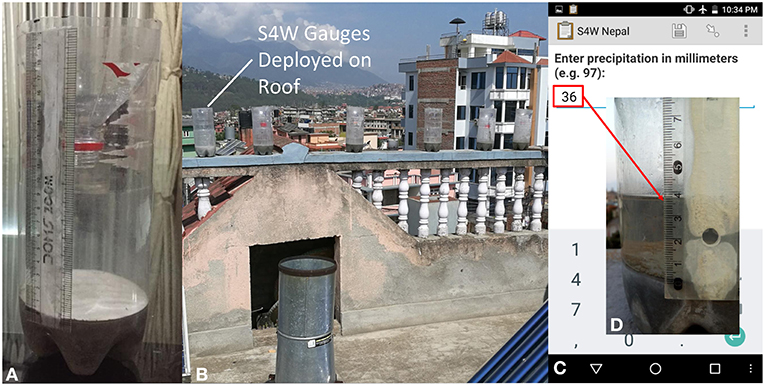
Figure 2. (A) Repurposed plastic bottle after placement of concrete, ruler, and inverted lid. (B) S4W Gauges installed on the roof of the S4W-Nepal office in Thasikhel, Lalitpur, Nepal. After selecting the parameter to measure, the citizen scientist (C) entered their observation of precipitation (mm) and (D) took a picture of the water level in the S4W rain gauge before emptying it. Each record was reviewed by S4W-Nepal staff to ensure that the numeric entry from the citizen scientist (C) matched the photographic record of the observation (D). Any observed discrepancies were corrected, and records of edits were maintained.

The S4W gauge design is similar to what Hendriks (2010) proposed as a low-budget rain gauge, except that the addition of a solid base and measuring scale enabled direct measurements of precipitation depths, thus eliminating the need to measure water volumes. Similar low-cost funnel-type gauges have also been used extensively in rainfall partitioning studies (Lundberg et al., 1997; Thimonier, 1998; Marin et al., 2000; Llorens and Domingo, 2007).

Precipitation measurements were performed by citizen scientists using an Android smartphone application called Open Data Kit Collect (ODK Collect; Anokwa et al., 2009). Video tutorials of how to install and use ODK and perform S4W precipitation measurements are available on S4W's YouTube channel (https://bit.ly/2Rdtadx; Nepali language only). Citizen scientists collected the precipitation data presented in this paper by performing the following steps:

1. S4W gauges were installed in locations with open views of the sky (e.g., Figure 2B).

a. Gauge heights above ground surface ranged from 1 meter (m) in rural areas to over 20 m (on rooftops) in densely populated urban areas.

2. An inverted lid without a cap (i.e., Cap1; see Evaporation errors) was used to minimize evaporation losses.

3. Measurements were performed as often as daily but sometimes less frequently.

4. Gauges were removed from their stands and placed on a level surface.

5. Precipitation readings were taken as the height of the lower meniscus of the water level within the bottle with the gauge placed on a level surface.

6. A numeric reading of precipitation level was entered into ODK in millimeters (mm; Figure 2C).

7. ODK was used to record a photograph of the water level with the smartphone camera level to the water surface (Figure 2D). ODK was also used to record date, time, and GPS coordinates.

8. Water was quickly dumped from the gauge to ensure that all ponded water above the concrete surface was removed but moisture within the concrete was retained.

9. The measurement was saved locally to smartphone memory and sent to the S4W-Nepal ODK Aggregate server running on Google App Engine.

(a) ODK was designed to work offline (i.e., without cellular connection) and can be configured to automatically or manually send data after the connection is restored.

Error Analysis

The World Meteorological Organization (WMO, 2008) identified the following primary error sources for precipitation measurements (estimated magnitudes in parentheses): evaporation (0–4%), wetting (1–15%), wind (2–10% for rain), splashing in or out of the gauge (1–2%), and random observational and instrument errors. The first three sources of errors are all systematic and negative (WMO, 2008). Because of the S4W gauge design, we separated wetting into concrete soaking and condensation on the clear plastic walls. The resulting categories of S4W gauge errors included: (1) evaporation, (2) concrete soaking, (3) condensation, and (4) other. Unlike some observation errors, which can be identified and corrected from photographs, gauge related errors must be understood and, if possible, systematically corrected. The following sections provide additional details regarding the first three sources of gauge errors related to the S4W gauge being low-cost and non-standard in nature. While all gauge errors were originally measured by differences in mass, all errors were converted to an equivalent depth (mm) for comparison. It should be noted that other rainfall gauge related errors, such as errors in construction of the gauge, errors related to placement of the gauge (e.g., a gauge installed too close to a building or below vegetation), or errors related to maintenance of the gauge (e.g., clogging) were not analyzed but are described in more detail below.

Evaporation errors

For manually read gauges, evaporation errors occur when precipitation evaporates from the rain gauge prior to taking a reading. Gauge design, weather, and the duration between precipitation events and gauge readings all impact the magnitude of the evaporation errors. To assess evaporation errors for S4W gauges, we performed evaporation tests between June 5th and August 23rd, 2018. We evaluated the impact of the following three rain gauge cover configurations on evaporation losses: (a) Open (i.e., no lid), (b) Cap1 (i.e., lid without cap), and (c) Cap2 (i.e., lid with cap and 7 mm hole; Figure 3). We randomly selected three gauges for each of these cover configurations for a total of nine gauges. With these nine gauges, we performed eleven sets of 24 h evaporation measurements yielding a total of 99 evaporation observations (i.e., 33 for each cover configuration).

FIGURE 3

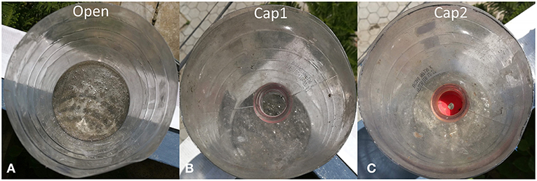
Figure 3. Three different rain gauge cover configurations for evaporation measurements. Open (A) is completely open to the atmosphere. Cap1 (B) has the original top of the bottle inverted and placed back on top of the gauge. Cap2 (C) has the same cover but also includes the original soda bottle cap with a 7 mm punched or drilled hole in the center to allow precipitation to enter the gauge. The resulting areas open to evaporation were roughly 7,850, 530, and 40 mm² for Open, Cap1, and Cap2 covers, respectively. The diameters of the cover and the lower portion of the gauge are the same, but the thickness of the plastic material causes a tight connection between the cover and the gauge.

We performed an initial investigation to see if the depth of water in the gauge had a noticeable impact on evaporation losses. We investigated two water depths (i.e., 10 and 30 mm) that corresponded to commonly observed rainfall events in the Kathmandu Valley. Our initial results showed that evaporation losses were not noticeably different between the 10 and 30 mm depths, so we used 30 mm depths for the remainder of the tests.

During each 24 h period, all nine gauges were set on the roof of the S4W-Nepal office in Thasikhel, Lalitpur (https://goo.gl/maps/oq81TwPAZnk) in a place with full exposure to the sun and wind. If precipitation occurred during the 24 h period, the experiment was canceled and restarted the following day. We used an EK1051 [Camry] electronic weighing scale (accuracy ± 1 g ≈ ± 0.08 mm) to determine evaporation losses by measuring the mass of the gauges before and after each successful (i.e., no precipitation) 24 h period.

Concrete soaking errors

As previously described, S4W gauges have a concrete base. As a semi-porous media, concrete requires a certain amount of moisture prior to saturation and subsequent ponding or accumulation of water above the concrete surface. The amount of water absorbed prior to ponding is a function of the concrete mixture (e.g., type and ratio of materials, etc.), the volume of concrete, and the initial moisture content of the concrete. The depth of precipitation read from S4W gauges represents only precipitation that accumulates above the concrete surface. Any precipitation that soaks into the concrete itself was not included in gauge readings. Therefore, concrete soaking represented a systematic negative error.

To evaluate soaking, we used an EK1051 [Camry] electronic weighing scale to measure the mass of the nine gauges used in the evaporation tests in both dry and saturated conditions. For the first set of measurements, the concrete had cured and dried for 30 days and no additional water beyond the amount initially needed for making the concrete mixture had been introduced to the gauge. To saturate the concrete, ~100 mm of water was added to the gauge and left for a period of 24 h. Subsequent soaking measurements were performed after drying the gauges in sunlight for periods ranging between one and 3 days.

Condensation errors

For S4W gauges with Cap1 and Cap2 covers, condensation accumulated on the clear plastics sides of the rain gauge. Because we used weight as a measurement to quantify evaporation losses, condensation was not included as a loss; only water that fully exited the rain gauge was considered an evaporation loss. However, water that evaporates and subsequently condenses on the gauge walls causes a lowering of the ponded water level, or the amount of moisture within the concrete if no ponded water is present. Therefore, condensation constitutes a systematic negative error in S4W gauge readings.

To evaluate condensation, we filled the same nine gauges with roughly 5 mm of water and covered them with a Cap2 cover. The gauges were placed in the sun for ~2 h to allow condensation to develop. Condensation was removed from gauges by wiping the inside of each gauge completely dry with a paper towel, ensuring that any remaining ponded water at the bottom was avoided. We determined condensation with an EHA501 [Camry] electronic weighing scale (accuracy ±0.1 g ≈ ±0.008 mm) by measuring the mass difference between each saturated and dry paper towel.

Other errors not included in this analysis

Differences in gauge installation can impact precipitation measurements. For example, gauge height can influence systematically negative wind-induced errors (Yang et al., 1998) or cause splash into the gauge. Wind-induced errors average between 2 and 10% and increase with decreasing rainfall rate, increasing wind speed, and smaller drop size distributions (Nešpor and Sevruk, 1999). Gauges that are not installed level will also cause an undercatch. The suitability of all gauge installation locations used in this paper were evaluated by S4W-Nepal staff by reviewing pictures of each gauge installation. Any issues identified from pictures were communicated directly to citizen scientists via personal communication (SMS, phone call, or site visit) and corrective actions were taken. However, installation errors are not the focus of this work and the data collected to date were insufficient to characterize these errors; therefore, gauge installation errors were not analyzed.

Gauge construction quality can also introduce errors. If future studies use gauges constructed by citizen scientists themselves (not the case in this study), the errors related to differences in construction quality should be considered.

Other possible maintenance or observation errors that may impact citizen scientists' measurements include: clogging of gauge inlets, incomplete emptying of gauges, and taking readings on unlevel surfaces. Effective training and follow-up is likely the key to minimizing such errors, so future work should explore different training approaches and their efficacy for various audiences. Training approaches should also consider scalability; for example, site visits become impractical if there are 1,000 participants.

Comparison to Standard Rain Gauges

To evaluate the accuracy of S4W gauges, a comparison with three other gauges (within 5 meters) was performed in Bhaisepati, Lalitpur, Nepal from May 1st, 2017 to April 30th, 2018 (Figure 4). Measurements were generally taken within 12 h of the end of each precipitation event, and in the morning or evening to minimize condensation errors. The other gauges included an Onset Computer Corporation Hobo Tipping Bucket RG3-M Rain Gauge (Onset), a manually read Community Collaborative Rain, Hail, and Snow Network standard gauge (CoCoRaHS), and a manually read standard 203 mm (8-inch) diameter Nepali Department of Hydrology and Meteorology gauge (DHM; similar to US National Weather Service 203 mm (8-inch) gauges). The Onset gauge measured the date and time of every 0.2 mm of precipitation from June 3rd to November 23rd, 2017.

FIGURE 4

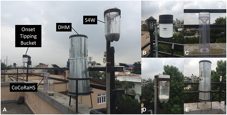
Figure 4. Comparison between (A) four different gauges including: (B) Onset Computer Corporation Hobo tipping bucket, (C) Community Collaborative Rain, Hail, and Snow Network (CoCoRaHS) standard 102 mm (4-inch) diameter gauge, (D) S4W gauge, and (E) the Nepali Department of Hydrology and Meteorology (DHM) standard 203 mm (8-inch) diameter gauge (similar to a US National Weather Service 203 mm (8-inch) gauge).

We used DHM gauge measurements as the reference or actual precipitation. Because Onset data were not available for the entire year period (i.e., May 1st, 2017 to April 30th), cumulative errors for the Onset gauge are not presented. Only fully overlapping data sets between DHM and Onset are used. Based on DHM measurements, we grouped the data into three precipitation event sizes (i.e., 0–5, 0–25, and 0–100 mm).

Recruiting and Motivating Citizen Scientists

Citizen science projects rely on citizens. As such, the success of any citizen science project relies at least partly on successful citizen recruitment and engagement efforts. We decided to focus monitoring on a 5-month period from May through the end of September in 2018. Even though the monsoon usually does not start until the middle of June (Ueno et al., 2008), starting the campaign in May provided time to ramp up interest and participation. Interested and motivated citizen scientists were encouraged to continue measurements after the campaign. We recruited citizen scientists for the monitoring campaign with a variety of methods (the number of citizen scientists recruited with each method is shown in parentheses):

• R1: Leveraging personal relationships (n = 53)—At the time of the 2018 monsoon expedition, the S4W-Nepal team was comprised of nine young researchers (i.e., BSc, MSc, and Ph.D. researchers or recent graduates). Our first round of citizen science recruiting started with our personal connections. Each of us asked our family, friends, and colleagues to consider joining the S4W-Nepal monsoon monitoring campaign.

• R2: Social media posts (n = 11)—We made posts on S4W's Facebook page (https://www.facebook.com/SmartPhones4Water) in order to explain the monsoon monitoring campaign and invite interested individuals to join as citizen scientists. S4W-Nepal's 2018 monsoon monitoring expedition titled “Count the Drops Before It Stops” included the main themes of “Join, Measure, and Change the way water is understood and managed in Nepal” (poster included as Supplementary Material).

• R3: Outreach programs at schools/colleges (n = 61)—In order to reach larger groups of possible citizen scientists, we organized outreach events at four secondary schools and five colleges during the spring of 2018. The outreach programs typically included presentations about the global water cycle, the Asian South Monsoon, the Kathmandu Valley water crisis, the importance of measuring resources we are trying to manage, and how the S4W-Nepal project is trying to quantitatively “tell the story” of the Valley's water problems to citizens and policy makers alike, with the aim to improve understanding and management in the future. Outreach programs generally ended with a call for volunteers, practical training on how to measure precipitation, and the distribution of S4W gauges to interested individuals. In the case of secondary schools, S4W gauges were provided to the schools directly, along with large pre-printed canvas graphs for plotting both daily precipitation amounts and cumulative monsoon precipitation totals.

• R4: Random site visits (n = 29)—The recruiting methods above mainly reached people living in the core urban areas of the Valley. However, our goal was to maximize the spatial distribution of our precipitation monitoring network, so it was important to include sites in the surrounding rural areas as well. In order to recruit citizen scientists in these areas, we made random site visits to strategic areas lacking citizen scientists. Sometimes during these random site visits, we would first talk to local community members to explain the vision and importance of the S4W-Nepal project. If community members responded positively, we would ask for references of individuals with a general interest in science and technology who had working Android smartphones. At other times, we started a dialogue directly with people we thought might be interested. In either case, once an individual with a working Android smartphone showed interest, we together installed an S4W gauge and performed initial training, including taking a first measurement together. In roughly 10 cases, we provided donated Android smartphones to individuals who were keenly interested in participating, but did not have a working smartphone.

To visualize recruitment progress, we developed a heatmap of the number of measurements performed showing time by week on the horizontal axis and (A) individual citizen scientists, (B) recruitment method, and (C) motivational method on the vertical axis. When computing grouped averages, zeroes were used for citizen scientists who did not take measurements in the respective weeks. We used the Mann-Whitney U test (Mann and Whitney, 1947) for the entire 22-week period to determine if a significantly different number of measurements were taken for all possible pairs of recruitment methods and between paid (see motivation M7 below for details on payments) and volunteer citizen scientists. Citizen scientist composition was defined by four categories including: (A) volunteer or paid, (B) gender, (C) age, and (D) education. For education, citizen scientists were classified based on the highest level of education they had either completed or were currently enrolled in.

Once a citizen scientist has been successfully recruited it is critical to motivate their continued involvement. Previous studies have shown that appropriate and timely feedback is a key motivation factor for sustaining citizen science (Buytaert et al., 2014; Sanz et al., 2014; Mason and Garbarino, 2016; Reges et al., 2016). Essentially, there were two different combinations of motivations for the volunteers (n = 117) and paid (n = 37) citizen scientists, respectively. Motivations M1 through M6 were applied to all volunteers; whereas, M1, M2, and M7 were applied to paid citizen scientists.

• M1: Personal follow-ups—At the end of each week, we reviewed the performance of each citizen scientist and developed plans for personal follow-ups for the subsequent week. Follow-ups focused on citizen scientists who had taken measurements in the last month but had not taken a measurement in the last 5 days, or citizen scientists making either unit or meniscus errors (see section Performance of Citizen Scientists). Personal follow-ups included (a) SMS messages, (b) phone calls, and (c) site visits. Roughly 20 site visits were made each week, amounting to an average of two visits per volunteer, and five (i.e., monthly) visits per paid citizen scientists during the 5-month campaign. During personal follow-ups, S4W-Nepal staff reiterated the importance of the work the citizen scientists were doing, and the difference that their measurements were making. Another purpose was to develop stronger personal relationships and develop a sense of being part of a larger community of people who are passionate about improving the way water resources are managed in Nepal.

• M2: Bulk SMS messages—At the end of each week we provided personalized bulk SMS messages to all citizen scientists who had taken measurements during the 2018 monsoon campaigns. The goals of the messages were to acknowledge the citizen scientists' contributions, to summarize their measurements in a meaningful way, and to reinforce that their data was making a difference. The personalized message read: “Hello from S4W-Nepal! From StartDate to EndDate you have taken NumberOfMeasurements totaling AmountOfPrecipitation mm. Your data is making a difference! https://bit.ly/2Rb15Uo” where StartDate was the beginning of the monsoon campaign, EndDate was the date of the citizen scientists' most recent measurement, NumberOfMeasurements was the number of measurements and AmountOfPrecipitation was the cumulative depth of presentation between StartDate and EndDate. The link at the end of the message was to S4W's Facebook page.

• M3: Outreach and workshops—Because Nepal is a collectivist or group society, we thought it was important to gather as an entire group at least once a year for a post-monsoon celebration. At this celebration, preliminary results from our efforts were presented and stories from the citizen scientists were shared. We also did follow-up visits to schools that measured precipitation.

• M4: Use of the data—S4W's aim is to share all of the data we generate, but our data portal is not finished yet. We encouraged citizen scientists to continue their participation by providing them with all the data generated by the monsoon monitoring campaign.

• M5: Lucky draws—We held a total of nine lucky draws (i.e., raffles) for gift hampers that included earphones, study lamp, wallet, movie ticket, and mobile balance credits. Only citizen scientists taking regular measurements (i.e., at least 50% of the time) were entered into the lucky draw.

• M6: Certificates of involvement—Especially for high school, undergraduate, and graduate students, certificates are important motivational factors because companies or organizations looking for new hires consider participation and employment certificates an important part of a candidate's resume. In order to get a certificate, citizen scientists had to take measurements for at least 50% of the days during the monsoon.

• M7: Payments—In some cases, especially in rural areas with limited employment opportunities, where the need for data was high, and the number of possible volunteers was low, S4W-Nepal compensated citizen scientists for measurements. For these citizen scientists, S4W-Nepal provided a small per observation transfer to their mobile phone account. Precipitation observations earned 25 Nepali Rupees (NPR; roughly 0.22 USD).

We used the number of measurements per citizen scientists as a simple indicator of the effectiveness of motivational efforts. For each group in each citizen scientist characteristic (i.e., volunteer or paid, gender, age, and education level), we used the Kruskal-Wallis H test (Kruskal and Wallis, 1952) to see if there were statistically significant differences (alpha level = 0.01) between the number of measurements taken by citizen scientists per group in each category per month during the entire 5-month period. For example, for age, we tested if more measurements per month were taken by ≤18 compared to both 19–25 and >25, and so forth.

Performance of Citizen Scientists

Using a custom Python web application, we manually reviewed pictures from every precipitation observation to ensure that values entered by citizen scientists (Figure 2C) matched photographic records (Figure 2D). Any observed discrepancies were corrected, and records of edits were maintained. Through this process we identified three categories of citizen science observation errors: unit, meniscus, and other errors. Unit errors caused an order of magnitude difference between original citizen scientist values and edited values due to citizen scientists taking readings in centimeters instead of millimeters. Meniscus errors were caused by citizen scientists taking readings of capillary rise instead of the lower portion of the meniscus, which was as much as 3 mm in some cases. Other observation errors were errors caused by unknown factors.

The combination of edit ratio and edit distance was used to determine the type of error for each corrected record. Edit ratio was calculated as:

$\begin{array}{ll}E{R}_i=\frac{O{V}_i}{E{V}_i}& (1)\end{array}$

where ER_i is the edit ratio, OV_i is the original precipitation value, and EV_i is the edited precipitation value for record i. Unit errors were defined as records with edit ratios between 8 and 12. Edit distance was calculated as:

$\begin{array}{ll}E{D}_i=O{V}_i-E{V}_i& (2)\end{array}$

where ED_i is edit distance for record i. Meniscus errors were defined as records with edit ratios <8 and edit distances between 0 and 3. The remaining edited records (neither unit nor meniscus errors) were classified as unknown observation errors.

On a weekly interval, we performed additional training and follow up (via SMS, phone, or in person) with citizen scientists who had made measurement errors during the previous week. Performance ratio was used to evaluate individual and group performance and was calculated as:

$\begin{array}{ll}P{R}_{CS,t}=\frac{TN{M}_{CS,t}-NC{M}_{CS,t}}{TN{M}_{CS,t}}\times 100\%& (3)\end{array}$

where PR_CS,t is the performance ratio for one or more citizen scientists (CS) during time period (t), NCM_CS,t is the number of corrected measurements, and TNM_CS,t is the total number of measurements for the same citizen scientist(s) (CS) and time period (t). Performance ratio (%) ranges from 0 to 100 with 100% being ideal.

We used the Mann-Whitney U test (Mann and Whitney, 1947) to evaluate if the interquartile range (IQR) of citizen scientists (in terms of the number of measurements they took) had worse performance ratios (PRs). After dividing citizen scientists into two groups based on the number of measurements they took during the 5 months campaign [i.e., (1) the IQR and (2) the remainder], we calculated the Mann-Whitney U on the PRs (alpha level = 0.01).

Cost per Observation

In order to evaluate the cost effectiveness of our approach, and any relationships between cost and citizen science performance, we performed a reconnaissance-level cost per observation (CPO) analysis. For each citizen scientist, average CPO was calculated as:

$\begin{array}{ll}CP{O}_{CS,t}=\frac{E{C}_{CS,t}+R{C}_{CS,t}+M{C}_{CS,t}}{TN{M}_{CS,t}}& (4)\end{array}$

where EC is equipment costs, RC is recruiting costs, MC is motivational costs, and TNM is the total number of measurements for each citizen scientist (CS) and time period (t). In this case, the time period was 5 months from May through September 2018. The following general assumptions were used for the CPO analysis:

• All costs (Table 1) are in Nepali rupees (NRP); an exchange rate of 114.3 NPR (November 22nd, 2018) per United States dollar (USD) was used for currency conversion

• All costs assume an hourly labor rate of 50 NPR per hour

• The full study period of 22 weeks was used for calculating costs unless stated otherwise

TABLE 1

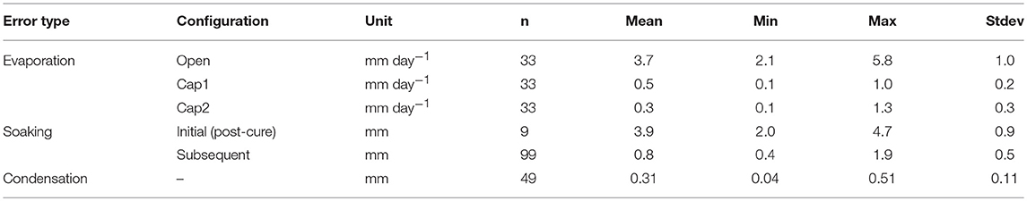
Table 1. Summary of the results from the evaporation, soaking, and condensation experiments (error type), including configuration, unit, sample size (n), mean, minimum (min), maximum (max), and standard deviation (stdev).

It is important to have a general sense of Nepal's economic context to properly interpret CPO results. Nepal's per capita gross domestic product (GDP) in 2018 was 1,004 USD or 114,800 NPR (CEIC, 2019). Assuming 2,080 working hours per year (i.e., 40 h work week for 52 weeks), the average hourly rate for 2018 was 0.48 USD or 55 NPR per hour.

All citizen scientists used the S4W gauge, so equipment costs were constant. RC was different for citizen scientists depending on which recruitment strategy (R1 through R4) was applied; we assumed that only one recruitment strategy was ultimately responsible for each citizen scientists' participation (recruitment methods per citizen scientist are included as Supplementary Material). Table 1 details the assumptions used to develop recruitment and motivational costs.

Motivational costs (MCs) for volunteers (MCVol) were entirely fixed, and were solved for using Equation 5. For paid citizen scientists, MCs were a combination of fixed (MCPaid; Equation 5) and variable costs (M7; Equation 6). MCs were calculated with the following equation:

$\begin{array}{ll}M{C}_{CS,t}=\{\begin{array}{cc}M{1}_a+M{1}_b+M{1}_{c}V+M2+M3+M4+M5+M6,& ifCSisVolunteer\\ M{1}_a+M{1}_b+M{1}_{c}P+M2+M{7}_{CS,t},& ifCSisPaid\end{array}& (5)\end{array}$

where the variables are defined above, with the exception of M7_{CS, t} for paid citizen scientists. M7_{CS, t} was calculated as:

$\begin{array}{ll}{M7}_{CS,t}=TN{M}_{CS,t}*R_{Precip}& (6)\end{array}$

where R_precip is the payment rate for each precipitation measurement. TNM_{CS, t} was limited to a maximum of one measurement per day.

Results

S4W Rain Gauge Results

Of the S4W gauge errors investigated (Table 2), initial (post-cure) concrete soaking errors (n = 9) and evaporation without lids (Open; n = 33) were the largest, averaging 3.9 mm and 3.7 mm day⁻¹, respectively. Subsequent concrete soaking requirements (n = 99) averaged 0.8 mm, or roughly five times smaller than the initial soaking requirement. S4W gauge evaporation was reduced from Open by an average of 86% (0.5 mm day⁻¹) and 92% (0.3 mm day⁻¹) for Cap1 and Cap2 configurations, respectively. Condensation errors were similar to Cap2 evaporation, and averaged 0.31 mm (n = 49).

TABLE 2

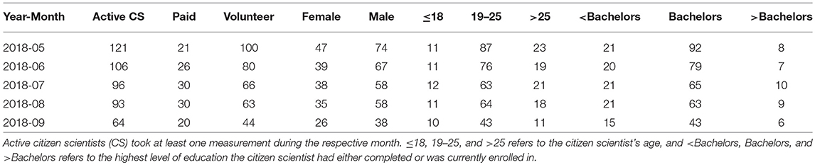
Table 2. Number and compositions of citizen scientists taking measurements from May through September 2018.

Cumulative precipitation amounts for the 1 year of data collected were 900, 930, and 927 mm for the S4W, CoCoRaHS, and DHM gauges, respectively. Using DHM as the reference for the entire year of data, cumulative gauge error was −2.9% for S4W and 0.3% for CoCoRaHS. Measured precipitation amounts were linearly correlated for the three precipitation ranges, but the correlation decreased in strength as total precipitation decreased (Figure 5). Points near the horizontal axis of Figure 5A (n = 9) indicate that some small rain events (n = 5 for DHM less than the 0.8 mm soaking loss; n = 4 for DHM between 0.8 and 2 mm) were completely missed by the S4W gauge.

FIGURE 5

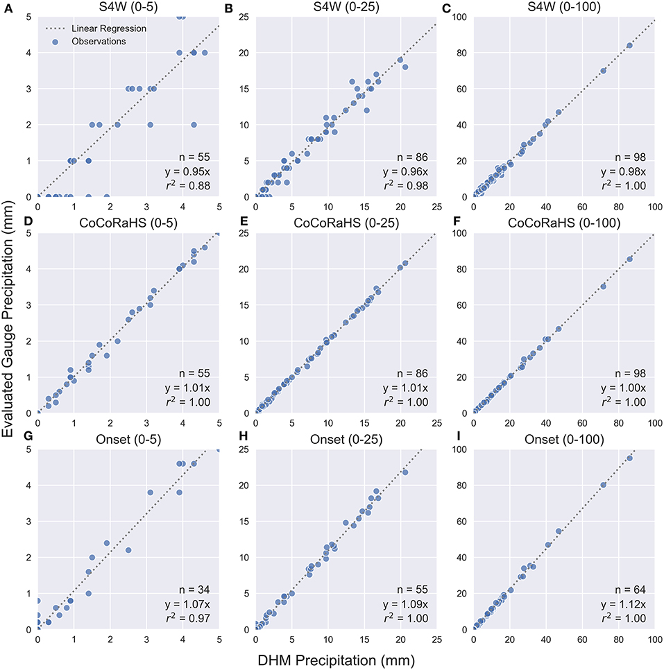
Figure 5. Comparison of precipitation data from S4W, CoCoRaHS, and Onset gauges using DHM observations as the reference (i.e., horizontal axis). Per reference DHM measurements, data was filtered into three precipitation event ranges: 0–5 mm [i.e. panels (A,D,G)], 0–25 mm [i.e., panels (B,E,H)], and 0–100 mm [i.e., panels (C,F,I)]. No precipitation events above 100 mm were recorded. Data shown are from May 1st, 2017 through April 30th, 2018. The period of record for the Onset gauge was June 3rd, 2017 to November 27th, 2018; only fully overlapping data sets between Onset and DHM were used, resulting in decreased sample sizes for panels (G–I).

For S4W, the magnitude of the systematic underestimation increased for smaller measurements (Figures 5A–C). For example, for precipitation measurements between 0 and 5 mm (Figure 5A), the S4W gauge linear regression coefficient was 0.95 indicating that measurements were on average −5% from the DHM gauge. In contrast, linear regression coefficients for 0 to 25 and 0 to 100 mm ranges were 0.96 (−4%) and 0.98 (−2%), respectively. Measurements from the CoCoRaHS gauge were strongly correlated with the measurements from the DHM gauge for all ranges with small biases (linear regression coefficients between 1.00 and 1.01; Figures 5D–F). For Onset, the magnitude of systematic overestimation increased for larger events (Figures 5G–I), from 1.07 (7%) at 0 to 5 mm, and up to 1.09 (9%) and 1.12 (12%) at 0 to 25 and 0 to 100 mm ranges, respectively.

Recruiting and Motivating Citizen Scientists Results

A heatmap of citizen scientists' precipitation measurements per week illustrates the rate of recruitment along with the continuity of their measurements (Figure 6A). “Citizen science heroes” can be seen as the persistent dark blue rows (e.g., the second row down from the top). In contrast, inconsistent citizen scientists can be seen as the rows with large variations in blue (e.g., fifth and sixth rows down from the top). Unfortunately, several citizen scientists took only a few measurements during their first week, especially toward the end of the second week (e.g., 2018-19). At a 0.05 alpha level, the average number of measurements per week was significantly higher for citizen scientists recruited via social media (R2) vs. personal relationships (R1; Figure 6B; p = 0.018), recruited via outreach programs (R3) vs. personal relationships (R1; Figure 6B; p = 0.033), and motivated with payments vs. volunteers (Figure 6C; p = 0.013). At an alpha level of 0.01, the average number of measurements per week was significantly higher for recruitment by random site visits (R4) vs. personal connections (R1; Figure 6B; p = 0.003). No other statistically significant differences (alpha level = 0.05) were observed between the remaining possible pairs of recruitment methods.

FIGURE 6

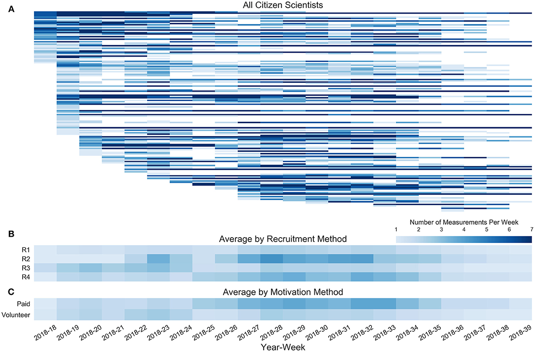
Figure 6. Heatmap of the number of measurements per year-week for a 22-week period from the first week of May (i.e., 2018-18) through the end of September (i.e., 2018-39). Each column of pixels represents a single week. Each row of pixels represents (A) an individual citizen scientist (n = 154), (B) averages from the four recruitment methods [i.e., R1: Leveraging personal relationships (n = 53); R2: Social media (n = 11); R3: Outreach programs (n = 61); R4: Random site visits (n = 29)], or (C) motivation method group [i.e., paid (n = 37) or volunteer (n = 117)]; see sections Recruiting and Motivating Citizen Scientists and Recruiting and Motivating Citizen Scientists Results for details). The color of each pixel represents the number of measurements performed each week. Light and dark blue represent one and seven measurements, respectively; white means zero measurements were performed that week. For panel (A) citizen scientists are sorted vertically in reverse chronological order by the date of their first measurement; the rate of recruitment is shown by the slope of the left edge of pixels in the heatmap—larger negative slopes (i.e., 2018-18 and 2018-19) represent higher recruitment rates. When computing grouped averages for panels (B,C), zeroes were used for citizen scientists that did not perform measurements in the respective weeks.

The number of active citizen scientists peaked in May (n = 121) and decreased through the campaign until September (n = 64; Table 3). The ratio of female to male citizen scientists remained relatively stable throughout the period (mean = 63%). From May to September, the number of volunteer citizen scientists decreased by 66%, whereas the number of paid citizen scientists only decreased by 5%. The most stable age group was ≤18, followed by 19–25, and finally >25. In terms of education, <Bachelors and >Bachelors were more stable than Bachelors, which decreased by 53%.

TABLE 3

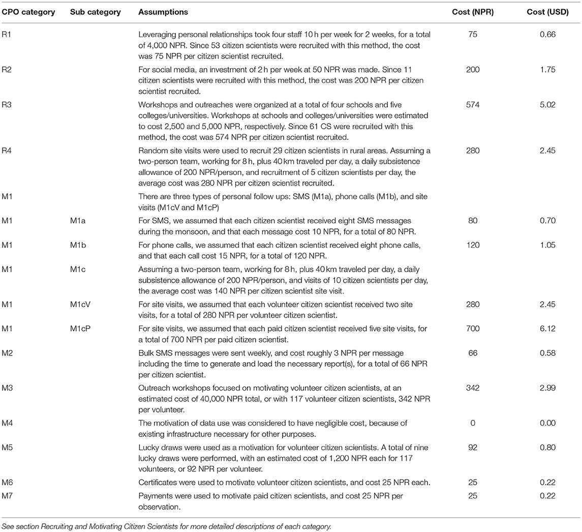
Table 3. Assumptions and the resulting costs for each recruitment and motivational category.

From May through September 2018, the average citizen scientist took 42 measurements (min = 1, max = 148, std = 39). Sixteen citizen scientists took only one measurement. Based on results from Kruskal-Wallis H tests, paid citizen scientists took significantly more measurements than volunteers (Figure 7; alpha level = 0.01; p = 0.005). No other statistically significant differences in contributions were observed.

FIGURE 7

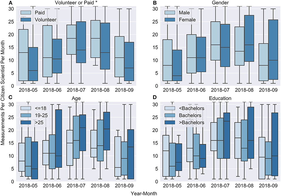
Figure 7. Grouped box plots showing the medians and distributions of the number of citizen scientist precipitation observations per month. Box plot groups are shown for four different categories: (A) volunteer or paid; (B) gender, (C) age, and (D) education. For education, citizen scientists were classified into the highest education level that they had either completed or were currently enrolled in. An asterisk (*) in the subplot title indicates statistically significant differences (alpha level = 0.01) between the number of measurements performed by each group within that category during the entire 5-month period.

There were statistically significant correlations between the number of measurements taken and mean daily precipitation for the same day (Figure 8A; r = 0.60; r critical = 0.21; alpha level = 0.01) and the previous day (Figure 8B; r = 0.38; r critical = 0.21; alpha level = 0.01), but the strength of the same day correlation was stronger, explaining 36% of the variance, while the previous day precipitation explained only 14%. This suggests that the harder it rains the more likely citizen scientists are to take a measurement that same day (and the next but less so).

FIGURE 8

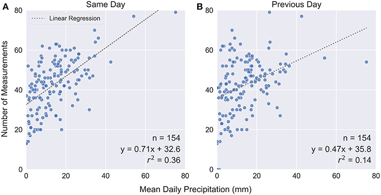
Figure 8. Scatter plot of the number of measurements per day as a function of mean daily precipitation for the (A) same day and (B) previous day. Mean daily precipitation was taken as the average of all citizen scientists' measurements. There were statistically significant correlations (Pearson's r) for the (A) same day (r = 0.60; r critical = 0.21; alpha level = 0.01) and the previous day (r = 0.38; r critical = 0.21; alpha level = 0.01).

Performance of Citizen Scientists Results

Citizen scientist observation errors were found for 9% (n = 592) of the total measurements (n = 6656). Meniscus errors (n = 346) (Figure 9; light blue area) accounted for 58% of observation errors. Unit errors (n = 50) (Figure 9; light red sector) comprised 8% of the errors. Finally, unknown errors (n = 196) accounted for the remaining 33% of observational errors.

FIGURE 9

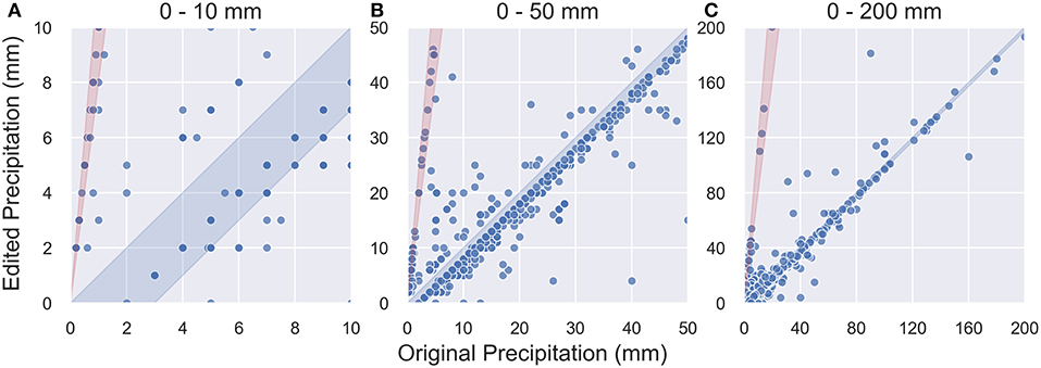
Figure 9. Scatter plot of corrected records (n = 592) with original (i.e., raw) precipitation entries on the horizontal axis and edited (i.e., after quality control) values on the vertical axis. Data is shown for three different scales: (A) 0–10 mm, (B) 0–50 mm, and (C) 0–200 mm. Meniscus error range (n = 346) is shown as light blue area, while Unit error range (n = 50) is shown as light red sector. Points outside of the light blue and light red areas are unknown errors (n = 196).

Only six citizen scientists had Unit, Meniscus, and Unknown errors. 41 citizen scientists had both Meniscus and Unknown errors; 10 had both Meniscus and Unit errors; and 8 had Unit and Unknown errors. The largest number of errors for a citizen scientist was 32, or 22% of their 143 records. The mean citizen scientist performance ratio (PR) was 93% (Figure 10). Stated alternatively, on average, there were errors on 7% of the measurements from citizen scientists. There were a total of 63 citizen scientists with perfect PRs (100%); 10 of these recorded more than the median number of measurements and 53 less (38 below Q1). Citizen scientists who took a moderate number of measurements (i.e., interquartile range (IQR) between Q1 and Q3; middle 50%) were significantly more likely to have a worse PR than those outside of the interquartile range (Figure 10; alpha level = 0.01; p = 0.0001).

FIGURE 10

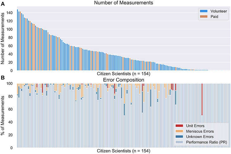
Figure 10. Summary of (A) the number of measurements collected from May through September with volunteer and paid citizen scientists distinguished and (B) the corresponding error composition for all 154 citizen scientists. Citizen scientists sorted in descending order by their total number of measurements. Performance ratio (PR) becomes less informative as the total number of measurements for each citizen scientist decreases, especially at or below two.

Cost per Observation Results

Fixed costs for equipment (S4W gauge) were 0.87 USD. Fixed costs for recruiting ranged from 0.66 to 5.02 USD, while for motivation they were 8.79 and 8.45 USD for volunteer and paid citizen scientists, respectively (Table 4; see Table 1 for details). Variable costs were only applicable for paid citizen scientists, and were 0.22 USD per observation. Outreach programs recruited the largest number of citizen scientists (n = 61), but were also the most expensive recruitment method (5.02 USD per citizen scientists recruited). Leveraging personal relationships was the second most effective (n = 53) and cheapest approach (0.66 USD). Random site visits recruited 29 citizen scientists, of whom 27 were paid, and cost roughly 2.45 USD per recruited citizen scientist. Only 11 citizen scientists joined the monitoring campaign purely through social media, for a cost of 1.75 USD per recruited citizen scientist.

TABLE 4

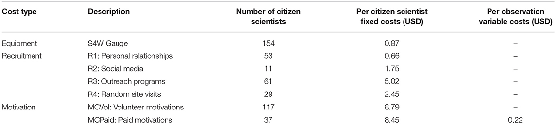
Table 4. Summary of fixed and variable costs for equipment, recruitment, and motivation per citizen scientist, including the number of applicable citizen scientists.

Estimated average costs per observation (CPO) for all citizen scientists ranged from 0.07 to 14.68 USD and 0.30 to 11.99 USD for volunteer and paid citizen scientists, respectively (Figure 11). Median CPOs where 0.47 USD for both volunteer and paid citizen scientists. Because all costs for volunteers are fixed, the number of observations per citizen scientist had the largest impact on CPOs. For example, volunteer citizen scientists (recruited with outreach programs) that took only one measurement had CPOs of 14.68 USD (Figure 11A). For paid citizen scientists, fixed costs were lower, but an additional variable cost of 0.22 USD (25 NPR) was added due to per observation payments. This resulted in a smaller range of CPOs, where (1) minimum CPOs approached per observation payment amount as the number of observations performed increased and (2) maximum CPOs approached fixed costs for paid citizen scientists as the number of measurements approached one (Figures 11C,D). Performance ratio (PR) did not appear to be related with CPO (Figures 11A,B).

FIGURE 11

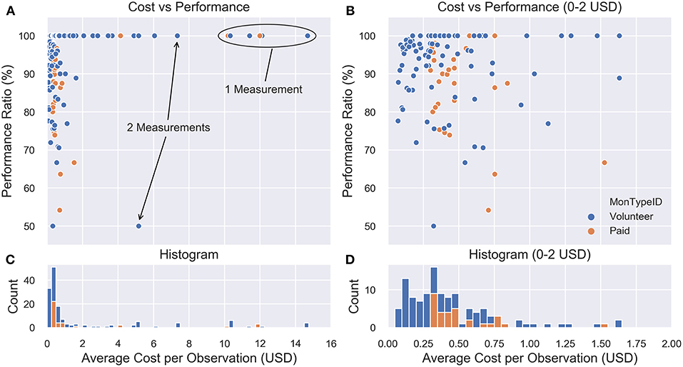
Figure 11. Scatter plots of performance ratio (PR) as a function of average cost per observation for costs from (A) 0–16 USD and (B) 0–2 USD ranges, respectively. Each point represents the performance ratio and average cost per observation for a single citizen scientist. Histograms below show the total number of citizen scientists in each cost bin for (C) 0–16 USD and (D) 0–2 USD ranges, respectively.

Gauge cost had a large impact on fixed costs for all citizen scientists. For example, increasing gauge cost from 0.87 USD (S4W gauge) to 31.50 USD (CoCoRaHS gauge) increased median CPOs from 0.47 to 1.57 and 1.12 USD for volunteer and paid citizen scientists, respectively. Using DHM gauges, which cost 65.60 USD, increases median CPOs to 2.88 and 1.85 USD for volunteer and paid citizen scientists, respectively. This analysis was limited to 5 months, however, since the estimated lifespan of all three gauges is well over 5 months (perhaps 5 years or longer), CPOs will decrease as more measurements are taken. As gauge lifespan increases, CPOs approach the sum of annually recurring fixed costs plus per observation variable costs.

Discussion

S4W Rain Gauge Discussion

In the context of wind induced errors arising from using (or not using) wind shields or differences in gauge heights, which can be as large as 10% for precipitation gauges of the same type (Sevruk and Klemm, 1989), the S4W gauge errors related to evaporation, soaking, and condensation are relatively small. Nevertheless, our findings highlight the importance of (1) using covers to minimize evaporation (regardless of cap type), in addition to (2) effective training on how to properly install covers to minimize air gaps and evaporation losses. Since evaporation can be limited by the amount of time that ponded water is stored in the gauge, citizen scientists should be encouraged to take measurements as quickly as possible after precipitation events. Citizen scientists should also be specifically guided to minimize the other errors discussed in section Error Analysis by: (1) keeping gauge inlets free of clogging hazards, (2) fully emptying gauges after measurements, and (3) taking readings on level surfaces.

Average S4W gauge evaporation losses with Cap1 (mean = 0.5 mm day⁻¹) and Cap2 (mean = 0.3 mm day⁻¹) compared favorably with Tretyakov gauge summer evaporation losses reported by Aaltonen et al. (1993), which ranged from 0.3 to 0.8 mm day⁻¹. Interestingly, Golubev et al. (1992) found evaporation losses from US National Weather Service 203 mm (8-inch) gauges (similar to the DHM gauge used in this investigation) to be “negligible” (e.g., 0.2 mm day⁻¹). While variability in evaporation can be partially explained by differences in solar radiation, wind speed, temperature, and relative humidity (Sevruk and Klemm, 1989), it is also possible that small differences in cover installation could also explain part of the observed variability in evaporation losses. For example, if a cover is installed at an angle, or not firmly pressed down, a small opening between the lid and the inside of the gauge can remain. These small openings could account for some of the high evaporation rates observed with Cap1 (max = 1.0 mm day⁻¹) and Cap2 (max = 1.3 mm day⁻¹) cover configurations (Table 2).

S4W gauges should be manually saturated prior to data collection to avoid the first roughly 3.9 mm of rain going to concrete saturation (Table 2). While subsequent saturation took only 0.8 mm, if not corrected for, this could introduce systematic negative bias into S4W gauge measurements. In order to reduce the need for corrections, alternative lower-porosity materials for filling the bottom of S4W gauges should be investigated.

Citizen scientists should be encouraged to take measurements at a consistent time in the morning (e.g., 07:00 LT; Reges et al., 2016) to minimize condensation errors and to simplify data processing. S4W gauge condensation averaged 0.31 mm, which is 61% of observed average daily Cap1 evaporation rates (0.5 mm day⁻¹) and 39% of concrete saturation requirements (0.8 mm). While percentage-wise, condensation errors were smaller than evaporation and concrete saturation, taking measurements in the morning (or evening) when condensation accumulations are low can reduce these errors. A correction for condensation errors could be added if the time of a measurement is during peak daylight hours.

While S4W gauge error was relatively small (−2.9%) compared to the DHM standard, it is still possible to apply corrections for the systematic S4W gauge errors. We suggest that corrections could be based on either an (1) error correction factor (ECF) or (2) evaporation (EVAP). The ECF uses cumulative precipitation values for S4W and DHM gauges to develop a constant correction, which is our case was 1.03. After adjusting S4W gauge records with the ECF approach, corrected cumulative S4W precipitation matched the DHM total of 927 mm. Alternatively, the EVAP approach is based on average daily evaporation (i.e., 0.5 mm) with soaking requirements (i.e., 0.8 mm) as an upper limit. After applying the EVAP approach, corrected cumulative S4W precipitation was 943 mm, or roughly 1.8% higher than DHM. Additional details regarding both of these approaches are included as Supplementary Material.

It is important to note that gauge errors, or systematic measurement differences, arising from differences in gauge installations were not evaluated. While standardizing gauge installation criteria like gauge height could help to minimize these differences, it may not be practical to apply such standards to citizen science projects in urban areas. For example, in the densely populated mid-rise core urban areas of Kathmandu, installing precipitation gauges at 1 m would only be possible in large courtyards. In these cases, it is likely more practical (and accurate) to install rain gauges on roof tops.

S4W gauge evaluation results should be considered the likely errors for “ideal” citizen scientists. Other possible errors that may impact citizen scientists' measurements include: (1) clogging of gauge inlets, (2) incomplete emptying of gauges, (3) improper gauge installation, and (4) taking readings on unlevel surfaces. Because we performed gauge intercomparison measurements ourselves with focused attention on avoiding these issues, they are not reflected in our results. Future work should consider the impacts of these potential error sources on citizen scientist measurements. Since it is likely that effective training and follow-up is the key to minimizing such errors, future work should also explore the effectiveness of different training approaches on different audiences.

Recruiting and Motivating Citizen Scientists Discussion

Our results showed that citizen scientists recruited via random site visits (R4; alpha = 0.01), social media (R2; alpha = 0.05), and outreach programs (R3; alpha = 0.05) on average took significantly more measurements than those recruited from personal connections (R1). Since all but two citizen scientists recruited from random site visits were also paid, it is not clear if the greater number of measurements was due to the recruitment method or payment, or a combination of the two. Citizen scientists who were recruited via social media had to take several self-initiated steps to move from (1) initially seeing something about S4W-Nepal on social media to (2) collecting precipitation data during the 2018 monsoon. In contrast, the barrier to entry for other recruitment methods was lower, and was externally initiated through interpersonal interactions. Therefore, the initial investment and motivation level of citizen scientists who joined the monitoring campaign through social media is relatively higher.

A survival analysis of volunteers in CoCoRaHS, the longest running large scale citizen science-based precipitation monitoring effort, found that retirement aged participants (i.e., ages 60 and above) were most likely to continue taking measurements (Sheppard et al., 2017). This suggests that older citizen scientists are most easily motivated, at least in a western context. While we did not have any retirement aged participants, our oldest age group (>25) actually had the largest attrition rates (52%). Future citizen science projects in Asia should focus on involving older citizen scientists to test the validity of this finding in the context of Nepal or other Asian settings.

Since payment appears to be an effective motivation, future work should explore how payment can be used as an effective means of recruitment. Also, recruitment of citizen scientists should be expanded to focus on retirement age groups and on clear communication of the usefulness of generated precipitation data.

While we only observed statistically significant differences in citizen science performance due to payment, roughly half of the bachelor's students involved in the project continued their involvement in the project (attrition rate was 53% for the 5 months campaign) without monetary motivations (no bachelor's students received payments). This suggests that students can be motivated to participate in citizen science projects with incentives like (1) the opportunity to use data for their research projects (e.g., bachelor's theses), (2) lucky draws (i.e., raffles or giveaways), and (3) by receiving certificates of involvement. However, these student-focused incentives often lead to data collection in urban areas, and may not be effective at generating data in rural areas with limited student populations and relatively low scientific literacy levels. In such areas, payments may be the most effective near-term incentive.

Survey results from CoCoRaHS volunteers have shown that a significant motivational factor is the knowledge that the data they are providing is useful (Reges et al., 2016). Therefore, a key component of any citizen science project should be “closing the loop” back to citizen scientists by clearly communicating the usefulness of their data, along with easy to understand examples. Our experience has shown that the difficulty of “closing the loop” increases as the citizen scientists' scientific literacy decreases. Therefore, in places like rural Nepal with, on average, relatively low scientific literacy rates, additional efforts must be made to properly contextualize and connect abstract concepts like data collection and fact-based decision making to the daily lives of community members. Payments might also be an important intermediate solution to motivate involvement while generational improvements in scientific literacy are realized.

Finally, even though we specifically reinforced the value of measuring zeros during training, our results suggested that the magnitude of precipitation was an important motivator for citizen scientists. However, there was some noise in this relationship because for the citizen scientists who did not take measurements, it was unknown whether this occurred because (1) there was no measurable precipitation in their gauge that day, or (2) they simply did not take a measurement. Regardless, this suggests that it may be difficult to motivate people to continue taking regular measurements outside the monsoon season, so focused monsoon monitoring campaigns are a good solution.

Performance of Citizen Scientists Discussion

Our findings reinforce the importance of including photographic records so that citizen science observations can be quality controlled and corrected if necessary. In our 5-month campaign, 9% of measurements required corrections; if not for photographic records, these errors may have been more difficult to detect, or may have gone unnoticed. It is important to note that the feedback we provided to citizen scientists about their errors during the campaign most likely led to fewer errors than there would have been without feedback. Future work should explore the opportunity to automate the quality control process by leveraging machine learning techniques to automatically retrieve correct values from photographs of measurements. Meniscus errors were more difficult to identify and correct from photographic records. Training citizen scientists to read the lower meniscus was at times a difficult task, because of the small variations in readings, often on the order of only a few millimeters.

Cost per Observation Discussion

Median CPOs of 0.47 USD for both volunteer and paid citizen scientists were roughly equivalent to 1 h of labor at nationally averaged rates (0.48 USD per hour; see section Cost per Observation for details). The cost per observation analysis revealed well over an order of magnitude difference between minimum and maximum average CPO for both volunteer and paid citizen scientists; this demonstrates the sensitivity of CPO to the number of observations. Our initial findings suggest that personal relationships and social media are the most cost-effective means of recruitment. A limitation of this study is that only two different groups of motivations were applied to volunteer and paid citizen scientists, respectively.

There was no increase in data accuracy with increases in CPO, thus efforts to minimize CPO do not appear to systematically lower PR. An important part of sustaining citizen science efforts is funding, and all efforts to minimize CPO while maintaining data quality will lead to lower funding requirements and greater chances of sustainability.

Since it is difficult to predict how citizen scientists will respond to recruitment and motivational efforts, returns on investments (as partially quantified by CPO) in citizen science monitoring efforts are uncertain and difficult to predict. Improved characterization of the effectiveness of different recruitment and motivational strategies will facilitate better understanding of the returns from citizen science-based precipitation monitoring investments.

Outlook

Using gauges constructed by citizen scientists could make citizen science rainfall monitoring approaches more scalable. However, if such gauges are used in future studies, the errors related to differences in construction quality should be evaluated. Since this study did not investigate potential gauge errors arising from (1) gauge clogging, (2) incomplete draining, (3) improper gauge installation, and (4) taking readings on unlevel surfaces, future work should focus on characterizing these errors. Additionally, the effectiveness of different training approaches aimed at minimizing such errors should be evaluated. Opportunities to automate the quality control review process used in this study (i.e., manual retrieval of correct rainfall values from photographs) should also be investigated.

While leveraging personal relationships was a cost-effective means of citizen scientist recruitment, relying on this method poses challenges to scalability. Future efforts should focus on development and refinement of more scalable approaches. We see young researchers (grade 8 through graduate school) as potential catalysts toward expanding and sustaining citizen science-based monitoring efforts. Future work should explore how sustainable measurements of precipitation (and other parameters) can be achieved by linking standard measurement goals and methods developed by professional scientists with (1) young researchers, (2) citizen science at the community level, and (3) a common technology platform including low-cost sensors (not necessarily electronic). Involving young researchers in this process has the potential benefits of both improving the quality of their education and level of practical experience, while simultaneously providing valuable data to support fact-based decision making. As previously mentioned (see section Recruiting and Motivating Citizen Scientists Discussion), the potential role of retired aged participants (i.e., ages 60 and above) in Asian citizen science projects, along with the possibility of using payment as a means of recruitment should also be investigated.

Finally, future efforts should explore the potential for cross-cutting organizations to facilitate and catalyze this process by linking young water-related researchers across a range of academic institutions related to water including: natural sciences, agriculture, engineering, forestry, economics, sociology, urban planning, etc. Desired outcomes of these links would be to (1) encourage young researchers to focus their efforts on relevant and multidisciplinary research topics and (2) encourage academic institutions to integrate participatory monitoring into their curricula and academic requirements (Shah and Martinez, 2016). Ultimately, these young researchers can then become the champions of engaging citizen scientists in the communities where they grew up, live, research, and work.

Conclusions

Our results illustrate the potential role of citizen science and low-cost precipitation sensors (e.g., repurposed soda bottles) in filling globally growing precipitation data gaps, especially in resource constrained environments like Nepal. Regardless of how simple low-cost gauges may be, it is critical to perform detailed error analyses in order to understand and correct, when possible, low-cost gauge errors. In this study, we analyzed three types of S4W gauge errors: evaporation (0.5 mm day⁻¹), concrete soaking (3.9 mm initial and 0.8 mm subsequent), and condensation (0.31 mm). Compared to standard DHM gauges, S4W and CoCoRaHS cumulative gauge errors were −2.9 and 0.3%, respectively, and were relatively small given the magnitude of other errors (e.g., wind induced) that affect all “catch” type gauges.

In total, 154 citizen scientists participated in the project, and on average performed 42 measurements (n = 6,656 total) during the 5-month campaign from May to September 2018. Citizen scientists recruited via random site visits, social media, and outreach programs (listed in decreasing order) took significantly more measurements than those recruited via personal connections. Payment was the only categorization (i.e., not gender, education level, or age) that caused a statistically significant difference in the number of measurements per citizen scientist, and was therefore an effective motivational method. We identified three categories of citizen science observation errors (n = 592; 9% of total measurements): unit (n = 50; 8% of errors), meniscus (n = 346; 58% of errors), and unknown (n = 196; 33% of errors). Our results illustrate that simple smartphone-based metadata like GPS-generated coordinates, date and time, and photographs are essential for citizen science projects. Estimated cost per observation (CPO) was highly dependent on the number of measurements taken by each participant and ranged from 0.07 to 14.68 USD and 0.30 to 11.99 USD for volunteer and paid citizen scientists, respectively. Median CPOs were 0.47 USD for both volunteer and paid citizen scientists. There was no increase in data accuracy with increases in CPO, thus efforts to minimize CPO do not appear to systematically lower citizen scientist performance.

Data Availability

The datasets generated and analyzed for this study can be found in the FigShare digital repository. All Python scripts used to analyze data and develop visualizations are included in the following GitLab repository: https://gitlab.com/jeff50/soda_bottle_science.

Author Contributions

JD had the initial idea for this investigation and designed the experiments in collaboration with MR, ND, AP, RP, and NvdG. Field work was performed by JD, AP, ND, and RP. JD prepared the manuscript with valuable contributions from all co-authors.

Funding

This work was supported by the Swedish International Development Agency (SIDA) under grant number 2016-05801 and by SmartPhones4Water (S4W).

Conflict of Interest Statement

The authors declare that the research was conducted in the absence of any commercial or financial relationships that could be construed as a potential conflict of interest.

Acknowledgments

Most importantly, we want to thank each and every citizen scientist who joined the S4W-Nepal family during our monsoon monitoring campaigns. This research would not be possible without them. We appreciate the dedicated efforts of Eliyah Moktan, Anurag Gyawali, Amber Bahadur Thapa, Surabhi Upadhyay, Pratik Shrestha, Anu Grace Rai, Sanam Tamang, Kristina M. Davids, and the rest of the S4W-Nepal team of young researchers. We would also like to thank Dr. Ram Devi Tachamo Shah, Dr. Deep Narayan Shah, and Dr. Narendra Man Shakya for their supervision and support of this work. Lastly, thanks to the reviewers for their useful comments.

Supplementary Material

The Supplementary Material for this article can be found online at: https://www.frontiersin.org/articles/10.3389/feart.2019.00046/full#supplementary-material

References

Aaltonen, A., Elomaa, E., Tuominen, A., and Valkovuori, P. (1993). “Precipitation measurement and quality control, v2,” in Proceedings of the International Symposium on Precipitation and Evaporation (Bratislava: Slovak Hydrometeorological Inst. and Swiss Federal Institute of Technology).

Anokwa, Y., Hartung, C., and Brunette, W. (2009). Open source data collection in the developing world. Computer 42, 97–99. doi: 10.1109/MC.2009.328

CrossRef Full Text | Google Scholar

Buytaert, W., Zulkafli, Z., Grainger, S., Acosta, L., Alemie, T. C., Bastiaensen, J., et al. (2014). Citizen science in hydrology and water resources: opportunities for knowledge generation, ecosystem service management, and sustainable development. Front. Earth Sci. 2, 1–21. doi: 10.3389/feart.2014.00026

CrossRef Full Text | Google Scholar

CEIC (2019). Nepal 2018 per Capita Gross Domestic Product (GDP). Available online at: https://www.ceicdata.com/en/indicator/nepal/gdp-per-capita (Accessed January 29, 2019).

Cifelli, R., Doesken, N., Kennedy, P., Carey, L. D., Rutledge, S. A., Gimmestad, C., et al. (2005). The community collaborative rain, hail, and snow network–informal education for scientists and citizens. Am. Meteorol. Soc. 86, 78–79. doi: 10.1175/BAMS-86-8-1069

CrossRef Full Text

Davids, J. C., Rutten, M. M., Pandey, A., Devkota, N., van Oyen, W. D., Prajapati, R., et al. (2018b). Citizen science flow – an assessment of citizen science streamflow measurement methods, Hydrol. Earth Syst. Sci. Discuss. 1:28. doi: 10.5194/hess-2018-425

CrossRef Full Text

Davids, J. C., Rutten, M. M., Shah, R. D. T., Shah, D. N., Devkota, N., Izeboud, P., et al. (2018a). Quantifying the connections—linkages between land-use and water in the Kathmandu Valley, Nepal. Environ. Monit. Assess. 190:304. doi: 10.1007/s10661-018-6687-2

PubMed Abstract | CrossRef Full Text | Google Scholar

Flohn, H. (1957). Large-scale aspects of the “summer monsoon” in South and East Asia. J. Meteor. Soc. Japan. 75, 80–186.

Google Scholar

Golubev, V. S., Groisman, P. Y., and Quayle, R. G. (1992). An evaluation of the United States standard 8-in. nonrecording raingage at the valdai polygon, Russia. J. Atmos. Ocean. Technol. 9, 624–629. doi: 10.1175/1520-0426(1992)009<0624:AEOTUS>2.0.CO;2

CrossRef Full Text | Google Scholar

Habib, E., Krajewski, W. F., and Kruger, A. (2001). Sampling errors of tipping-bucket rain gauge measurements. J. Hydrol. Eng. 6, 159–166. doi: 10.1061/(ASCE)1084-0699(2001)6:2(159)

CrossRef Full Text | Google Scholar

Hendriks, M. R. (2010). Introduction to Physical Hydrology. New York, NY: Oxford University Press.

Google Scholar

Hut, R. (2013). New Observational Tools and Datasources for Hydrology [dissertation]. [Delft (NL)]: Delft University of Technology. doi: 10.4233/uuid:48d09fb4-4aba-4161-852d-adf0be352227

CrossRef Full Text

Illingworth, S. M., Muller, C. L., Graves, R., and Chapman, L. (2014). UK citizen rainfall network: a pilot study. Weather 69, 203–207. doi: 10.1002/wea.2244

CrossRef Full Text | Google Scholar

Kidd, C., Becker, A., Huffman, G. J., Muller, C. L., Joe, P., Skofronick-Jackson, G., et al. (2017). So, how much of the Earth's surface is covered by rain gauges? Bull. Am. Meteorol. Soc. 98, 69–78. doi: 10.1175/BAMS-D-14-00283.1

PubMed Abstract | CrossRef Full Text | Google Scholar

Koutsouris, A. J., Chen, D., and Lyon, S. W. (2016). Comparing global precipitation data sets in eastern Africa: a case study of Kilombero Valley, Tanzania. Int. J. Climatol. 36, 2000–2014. doi: 10.1002/joc.4476

CrossRef Full Text | Google Scholar

Krajewski, W. F., Ciach, G. J., and Habib, E. (2003). An analysis of small-scale rainfall variability in different climatic regimes. Hydrol. Sci. J. 48, 151–162. doi: 10.1623/hysj.48.2.151.44694

CrossRef Full Text | Google Scholar

Kruskal, W. H., and Wallis, W. A. (1952). Use of ranks in one-criterion variance analysis. J. Am. Stat. Assoc. 47, 583–621. doi: 10.1080/01621459.1952.10483441

CrossRef Full Text | Google Scholar

Lettenmaier, D. P., Alsdorf, D., Dozier, J., Huffman, G. J., Pan, M., and Wood, E. F. (2017). Inroads of remote sensing into hydrologic science during the WRR era. Water Resour. Res. 51, 7309–7342. doi: 10.1002/2015WR017616

CrossRef Full Text | Google Scholar

Llorens, P., and Domingo, F. (2007). Rainfall partitioning by vegetation under Mediterranean conditions. a review of studies in Europe. J. Hydrol. 37–54. doi: 10.1016/j.jhydrol.2006.10.032

CrossRef Full Text | Google Scholar

Lundberg, A., Eriksson, M., Halldin, S., Kellner, E., and Seibert, J. (1997). New approach to the measurement of interception evaporation. J. Atmos. Ocean. Technol. 14, 1023–1035. doi: 10.1175/1520-0426(1997)014<1023:NATTMO>2.0.CO;2

CrossRef Full Text | Google Scholar

Mann, H. B., and Whitney, D. R. (1947). On a test of whether one of two random variables is stochastically larger than the other. Ann. Math. Stat. 50–60. doi: 10.1214/aoms/1177730491

CrossRef Full Text | Google Scholar

Marin, C. T., Bouten, W., and Sevink, J. (2000). Gross rainfall and its partitioning into throughfall, stemflow and evaporation in four forest ecosystems in northwest. J. Hydrol. 237, 40–57. doi: 10.1016/S0022-1694(00)00301-2

CrossRef Full Text

Mason, C. E., and Garbarino, J. (2016). The power of engaging citizen scientists for scientific progress. J. Microbiol. Biol. Educ. 17, 7–12. doi: 10.1128/jmbe.v17i1.1052

PubMed Abstract | CrossRef Full Text | Google Scholar

McKinley, D. C., Miller-Rushing, A. J., Ballard, H. L., Bonney, R., Brown, H., Cook-Patton, S. C., et al. (2017). Citizen science can improve conservation science, natural resource management, and environmental protection. Biol. Conserv. 208, 15–28. doi: 10.1016/j.biocon.2016.05.015

CrossRef Full Text | Google Scholar

Nayava, J. L. (1974). Heavy monsoon rainfall in Nepal. Weather 29, 443–450. doi: 10.1002/j.1477-8696.1974.tb03299.x

CrossRef Full Text | Google Scholar

Nayava, J. L. (1980). Rainfall in Nepal. Himal. Rev. Nepal Geogr. Soc. 12, 1–18.

Google Scholar

Nešpor, V., and Sevruk, B. (1999). Estimation of wind-induced error of rainfall gauge measurements using a numerical simulation. J. Atmos. Ocean. Technol. 16, 450–464. doi: 10.1175/1520-0426(1999)016<0450:EOWIEO>2.0.CO;2

CrossRef Full Text | Google Scholar

Pokharel, A. K., and Hallett, J. (2015). Distribution of rainfall intensity during the summer monsoon season over Kathmandu, Nepal. Weather 70, 257–261. doi: 10.1002/wea.2544

CrossRef Full Text | Google Scholar

Pokharel, B., Marahatta, S., Giri, B., and Stahl, P. (2016). CORAM-Nepal Website. Available online at: http://coramnepal.org/about-coram/

Reges, H. W., Doesken, N., Turner, J., Newman, N., Bergantino, A., and Schwalbe, Z. (2016). CoCoRaHS: the evolution and accomplishments of a volunteer rain gauge network. Bull. Am. Meteorol. Soc. 97, 1831–1846. doi: 10.1175/BAMS-D-14-00213.1

CrossRef Full Text | Google Scholar

Sanz, F. S., Holocher-Ertl, T., Kieslinger, B., García, F. S., and Silva, C. G. (2014). White Paper on Citizen Science in Europe. Available online at: http://www.socientize.eu/sites/default/files/white-paper_0.pdf

Sevruk, B., and Klemm, S. (1989). Instruments and observing methods (Report No. 39)–catalogue of national standard precipitation gauges. Geneva, Switzerland. Available online at: http://www.wmo.int/pages/prog/www/IMOP/publications/IOM-39.pdf

Shah, H. R., and Martinez, L. R. (2016). Current approaches in implementing citizen science in the classroom. J. Microbiol. Biol. Educ. 17, 17–22. doi: 10.1128/jmbe.v17i1.1032

PubMed Abstract | CrossRef Full Text | Google Scholar

Sheppard, S. A., Turner, J., Thebault-Spieker, J., Zhu, H., and Terveen, L. (2017). Never too old, cold or dry to watch the sky. Proc. ACM Hum. Comput. Interact. 1, 1–21. doi: 10.1145/3134729

CrossRef Full Text | Google Scholar

Shrestha, M. L. (2000). Interannual variation of summer monsoon rainfall over Nepal and its relation to southern oscillation index. Meteorol. Atmos. Phys. 75, 21–28. doi: 10.1007/s007030070012

CrossRef Full Text | Google Scholar

SRTM (2000). Shuttle Radar Topography Mission. Available online at: https://earthexplorer.usgs.gov/ (Accessed September 14, 2016).

Sun, Q., Miao, C., Duan, Q., Ashouri, H., Sorooshian, S., and Hsu, K. L. (2018). A review of global precipitation data sets: data sources, estimation, and intercomparisons. Rev. Geophys. 56, 79–107. doi: 10.1002/2017RG000574

CrossRef Full Text | Google Scholar

Tauro, F., Selker, J., Van De Giesen, N., Abrate, T., Uijlenhoet, R., Porfiri, M., et al. (2018). Measurements and observations in the XXI century (MOXXI): innovation and multi-disciplinarity to sense the hydrological cycle. Hydrol. Sci. J. 63, 169–196. doi: 10.1080/02626667.2017.1420191

CrossRef Full Text | Google Scholar

Thapa, B. R., Ishidaira, H., Pandey, V. P., and Shakya, N. M. (2017). A multi-model approach for analyzing water balance dynamics in Kathmandu Valley, Nepal. J. Hydrol. Reg. Stud. 9, 149–162. doi: 10.1016/j.ejrh.2016.12.080

CrossRef Full Text | Google Scholar

Thimonier, A. (1998). Measurement of atmospheric deposition under forest canopies: Some recommendations for equipment and sampling design. Environ. Monit. Assess. 52, 353–387. doi: 10.1023/A:1005853429853

CrossRef Full Text | Google Scholar

Turner, A. G., and Annamalai, H. (2012). Climate change and the South Asian summer monsoon. Nat. Clim. Chang. 2, 587–595. doi: 10.1038/nclimate1495

CrossRef Full Text | Google Scholar

Ueno, K., Toyotsu, K., Bertolani, L., and Tartari, G. (2008). Stepwise onset of monsoon weather observed in the Nepal Himalaya. Mon. Weather Rev. 136, 2507–2522. doi: 10.1175/2007MWR2298.1

CrossRef Full Text | Google Scholar

Villarini, G., Mandapaka, P. V., Krajewski, W. F., and Moore, R. J. (2008). Rainfall and sampling uncertainties: a rain gauge perspective. J. Geophys. Res. Atmos. 113, 1–12. doi: 10.1029/2007JD009214

CrossRef Full Text | Google Scholar

Volkmann, T. H. M., Lyon, S. W., Gupta, H. V., and Troch, P. A. (2010). Multicriteria design of rain gauge networks for flash flood prediction in semiarid catchments with complex terrain. Water Resour. Res. 46, 1–16. doi: 10.1029/2010WR009145

CrossRef Full Text | Google Scholar

WMO (2008). Guide to Meteorological Instruments and Methods of Observation. WMO-No. 8. Geneva, Switzerland: World Meteorological Organization Available online at: https://library.wmo.int/pmb_ged/wmo_8_en-2012.pdf

Yang, D., Goodison, B. E., Metcalfe, J. R., Golubev, V. S., Bates, R., Pangburn, T., et al. (1998). Accuracy of NWS 8″ standard nonrecording precipitation gauge: Results and application of WMO intercomparison. J. Atmos. Ocean. Technol. 15, 54–68. doi: 10.1175/1520-0426(1998)015<0054:AONSNP>2.0.CO;2

CrossRef Full Text | Google Scholar