Modeling the Response of the Langtang Glacier and the Hintereisferner to a Changing Climate Since the Little Ice Age

Introduction

Ongoing global warming has resulted in the retreat of glaciers over the last decades with important consequences for the society and the environment. Glacier mass loss has contributed to global sea-level rise (Radić and Hock, 2011; Gregory et al., 2013) and seasonal changes in river discharge (Kaser et al., 2010; Immerzeel et al., 2012; Lutz et al., 2014; Beniston et al., 2018; Hanzer et al., 2018; Huss and Hock, 2018). In addition, glacier retreat will most likely lead to natural hazards as a result of the destabilization of mountain slopes and hanging glaciers or the development of moraine-dammed lakes (Frey et al., 2010; Faillettaz et al., 2015; Haeberli et al., 2017).

Global glacier retreat started at the end of the Little Ice Age (LIA), which terminated globally around 1850 (Leclercq et al., 2011) and coincided with the Industrial Revolution that led to an increase in the emission of greenhouse gasses. Since the glacier area/length response to climate change has a lag of several decades (Johannesson et al., 1989; Adhikari et al., 2011; Banerjee and Shankar, 2013; Banerjee, 2017) it is difficult to unambiguously attribute glacier retreat to anthropogenic causes (Marzeion et al., 2014). In the nineteenth century, the anthropogenic influence on the climate system was limited, which therefore could not be the main cause of glacier mass losses (Myhre et al., 2013). Over the twentieth century, however, the anthropogenic influence increased rapidly as a result of the ongoing industrialization, in particular after the 1970s (Myhre et al., 2013). These increases have resulted in the anthropogenic climate signal becoming a prevailing explanation for the observed decrease in glacier mass since the 1980s (Marzeion et al., 2014; Hirabayashi et al., 2016).

Until now, the anthropogenic and natural influences on historical glacier changes have mainly been investigated in studies with a focus on changes in glacier mass balance (Marzeion et al., 2014; Hirabayashi et al., 2016). Several studies have, however, found a relation between glacier dynamics and thinning rates on glaciers (Huss et al., 2007; Berthier and Vincent, 2012; Banerjee, 2017; Dehecq et al., 2019). For example, Berthier and Vincent (2012) found that accelerated thinning rates during the last decades on the Mer de Glace Glacier, a partially debris-covered glacier in France, could partly be attributed to reduced ice fluxes. A more recently published study on glacier slowdown in High Mountain Asia (Dehecq et al., 2019) revealed that glaciers in most parts of the region show a sustained slowdown that is associated with ice thinning. Also, the authors found stable or increased ice flow in the regions around the Tibetan Plateau and the Tarim river basin where stable or positive mass balances are observed. Banerjee (2017) found that thinning rates on both debris-covered and clean-ice glaciers were dependent on the relation between mass balance changes and ice flux changes. Clean-ice glaciers show a different response to climate change than debris-covered glaciers because the supraglacial debris generally insulates the ice (Østrem, 1959; Nicholson and Benn, 2006; Reid and Brock, 2010; Jouvet et al., 2011; Rowan et al., 2015). On clean-ice glaciers, larger thinning rates are caused by a combination of reduced ice flow and a negative surface mass balance, which correspond to receding termini. On debris-covered glaciers, on the other hand, the negative mass balance is rather small due to insulation of the surface, which in combination with a reduced ice flow result in surface lowering, but without an considerable retreat of the glacier terminus (Naito et al., 2000; Hambrey et al., 2009; Banerjee and Shankar, 2013; Rowan et al., 2015; Banerjee, 2017). To understand the response of both types of glaciers to climate change, it is therefore necessary to make a proper coupling between mass balance models and ice flow models that have a sufficient representation of glacier dynamics (Huss et al., 2007; Adhikari and Marshall, 2013; Clarke et al., 2015; Shea et al., 2015).

Existing ice flow models vary between simple flowline models (Greuell, 1992; Van De Wal and Oerlemans, 1995; Span et al., 1997; Oerlemans et al., 1998; Huss et al., 2007; Adhikari and Huybrechts, 2009; Aðalgeirsdóttir et al., 2011; Banerjee and Shankar, 2013) and spatially-distributed three-dimensional higher-order or Stokes models (Leysinger Vieli and Gudmundsson, 2004; Jouvet et al., 2011; Seroussi et al., 2011; Adhikari and Marshall, 2012a, 2013; Jouvet and Funk, 2014; Zekollari et al., 2014). A simple description of glacial ice deformation is provided by the so-called Shallow Ice Approximation (SIA) of Stokes equations (Hutter, 1983), where ice flow can be obtained from a local gradient in glacier surface elevation and ice thickness (Egholm et al., 2011). This approach has the main advantage that the computational cost and data demand are low in comparison with the more complex higher-order or Stokes models, and is therefore useful in large-scale studies of glacier dynamics in data-scarce regions, such as High Mountain Asia. In addition, the approach enables the calibration and validation against observed surface velocities (e.g., those derived from satellite-based imagery) more readily. For large-scale applications, glacier flow is also represented using a simpler approach that assumes basal sliding, such as the one described by Weertman's sliding law (Weertman, 1957), to be the main driver of glacial movement. Many glaciers, however, are driven by a combination of internal deformation and basal sliding, which therefore hampers the calibration and validation of modeling approaches that solely rely on basal sliding laws (Nye, 1965; Cuffey and Paterson, 2010; Adhikari and Marshall, 2013). SIA models, by design, assume the dominance of vertical shear stress at the ice/bed interface and ignore higher-order stresses that describe lateral and longitudinal drags, which might limit its use on fast-flowing or steep/narrow valley glaciers (Le Meur et al., 2004; Adhikari and Marshall, 2013). To overcome this drawback, higher-order perturbative corrections to shallow ice models may be considered (Egholm et al., 2011; Rowan et al., 2015). However, the implementation of such corrections increases numerical complexity. Therefore, to account for the higher-order physics, correction factors are used that can sustain the simplicity of SIA models and yet obtain more realistic results at the same time (Nye, 1965; Adhikari and Marshall, 2011, 2012b).

Many models based on the SIA have been applied as flowline models (Adhikari and Huybrechts, 2009; Banerjee and Shankar, 2013). Although these types of models are easy to apply, they still require a priori knowledge of the number and orientation of flowlines on glaciers. This can be a disadvantage when applied over longer timescales (i.e., due to the varying orientation of flowlines over time) or at a larger spatial scale (i.e., when a larger number of flowlines is required to represent realistic dynamics of glaciers), which eventually reduces the compatibility of flowline models with gridded regional-scale hydrological models. In this context, spatially-distributed SIA models can be useful. As these models simulate the two-dimensional flow of ice, a priori information about flowline geometry is not required. These spatially-distributed SIA models are useful in simulating the evolution of the boundary and hypsometry of glaciers that naturally allows the feedbacks between glacier dynamics and mass balance forcing to be taken into account. Spatially-distributed SIA models should be invaluable for the accurate and efficient representation of glaciers in gridded regional-scale hydrological models (e.g., Immerzeel et al., 2012, 2013; Shea et al., 2015).

The main aim of this study is to develop and apply a spatially-distributed coupled glacier mass balance and dynamical ice-flow model toward understanding the response of glaciers to natural and anthropogenic climate change. We focus on two glaciers with contrasting surface characteristics: the Hintereisferner, which is a clean-ice glacier located in the European Alps, and the Langtang Glacier, which is a debris-covered glacier located in the Central Himalayas. We apply the model from the end of the LIA (1850) to the present-day (2016) and force the model with the outputs of four bias-corrected General Circulation Models (GCMs) that were pre-selected from the historical experiment of the Coupled Model Intercomparison Project Phase 5 (CMIP5). For the selected GCMs we selected runs with and without further anthropogenic forcing from 1971 onwards to separately assess the effects of anthropogenic climate change on glacier mass balance and flow. The novelty of this study in comparison with previous works in the two regions is its attribution of the response of two contrasting glaciers (i.e., in terms of surface characteristics) to natural and anthropogenic historical climate change using a coupled glacier mass balance and dynamical ice-flow model.

Study Area

We focus on two glaciers: the Langtang Glacier (Central Himalayas, Nepal), and the Hintereisferner (Central Eastern Alps, Austria) (Figure 1).

FIGURE 1

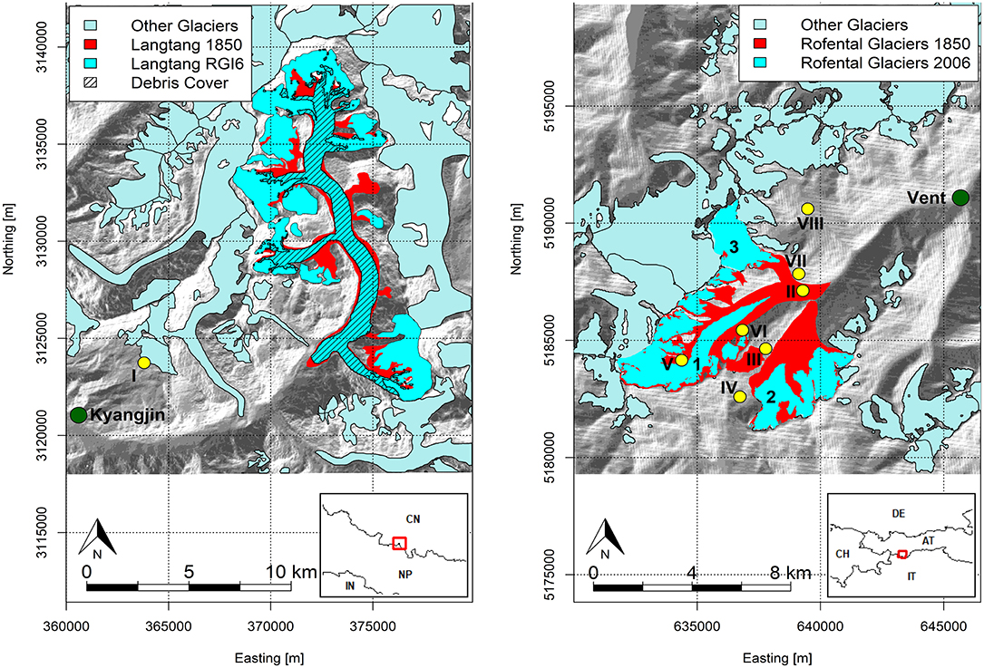
Figure 1. The Langtang Glacier (left) and Hintereisferner (right) with the glacier outlines of 1850 (turquoise), the current glacier outlines (red), and the current debris extents (black stripes; Langtang Glacier). The other glaciers (light blue) and the locations of the primary and secondary meteorological stations (green and yellow dots, respectively) in the region are also shown. The numbers 1, 2, and 3 denote the locations of the Hintereisferner, Hochjochferner, and Kesselwandferner, respectively. The numbers I–VIII denote the locations of the Yala base camp (I), Hochjochhospiz (II), Latschbloder (III), Bella Vista (IV), Hintereis (V), Rofenberg (VI), Proviantdepot (VII), and Vernagtbrücke (VIII) stations. Source of the glacier outlines are the Randolph Glacier Inventory v6 (Pfeffer et al., 2014) and the Austrian glacier inventories (Abermann et al., 2009; Fischer et al., 2015). The debris extents are obtained from Kraaijenbrink et al. (2017).

Langtang Glacier (28.296972 °N 85.709775°E) is a debris-covered valley glacier, which is located ~70 km north of Kathmandu. The glacier has a length of ~18 km and covers an area of 46.5 km² (2006; Ragettli et al., 2016). The elevation ranges from 4370 m a.s.l. at the terminus to 7119 m a.s.l. in the northernmost part of the catchment. The glacier surface slope varies from 4 to 88% with a mean of 32%. About 35% of Langtang Glacier is covered with debris, where most of the debris can be found in the ablation areas below 5200 m. a.s.l. The transition from debris-covered to clean-ice surfaces is very short and the heterogeneous surface of the Langtang Glacier is characterized by scattered ice cliffs and supraglacial ponds throughout all seasons (Ragettli et al., 2016; Steiner et al., in review). The climate in the Langtang Valley is dominated by the Indian monsoon with predominant easterly winds during the monsoon period and westerly winds from October to May (Immerzeel et al., 2012). During the monsoon period, more than 70% of the annual precipitation falls, whereas winters are relatively dry (Immerzeel et al., 2012; Collier and Immerzeel, 2015). In general, precipitation decreases with altitude during the monsoon season, whereas during the winter season precipitation increases with altitude (Collier and Immerzeel, 2015). The mean daily temperature at Kyangjin meteorological station (3930 m a.s.l.; located ~12 km from Langtang Glacier) is 4.0°C, and the mean annual precipitation sum 665 mm (over 1988–2016).

Hintereisferner (46.798814°N 10.770068°E) is a clean-ice valley glacier located in the upper part of the Rofental, Ötztal Alps, Austria. The glacier has a long record of investigations with the first measurements dating from 1894 and is classified as a “reference glacier” by the World Glacier Monitoring Service. This means that glacier changes are mainly driven by climate inputs and are not subject to other major influences, such as heavy debris cover, avalanching, surging, ice calving, or artificial snow (WGMS, 2018). The glacier has a length of approximately 7 km and an area of 7.4 km² (2006; Charalampidis et al., 2018). The total area of glaciers (including the adjacent Kesselwandferner and Hochjochferner) amounts to 19.5 km². During the LIA, the length of the Hintereisferner reached up to about 10 km. Further, the Kesselwandferner used to be linked with the Hintereisferner, but has been detached since the 1920s (Kuhn et al., 1985). The elevation ranges from 2238 m a.s.l. at the LIA terminus of the Hintereisferner to 3661 m a.s.l. The glacier surface slope varies from <1 to 78% with a mean of 25%. The climate in the Rofental can be characterized as a dry inner alpine climate with the lowest precipitation sums during winter (~125 mm) and the highest precipitation sums during summer (~265 mm) at the meteorological station in Vent (1,900 m a.s.l.; located ~10 km from the Hintereisferner) (over 1987–2016). The mean annual precipitation sum amounts to 750 mm and the higher annual precipitation sums (>1,500 mm) are mainly measured at the higher altitudes around 3000 m a.s.l. (Strasser et al., 2018). The annual average temperature at the meteorological station in Vent is 3°C (over 1988–2016).

Data and Methods

Historical and Reference Daily Climate Forcing

The glacier mass balance and ice-flow model is forced with climate data for the period 1851–2016. The forcing consists of two datasets: observed climate data derived from local meteorological stations and modeled climate data derived from GCM outputs.

The observed climate data consists of daily precipitation and mean air temperature data extracted from the Vent and Kyangjin stations for a 30-year period (1987–2016) and a 29-year period (1988–2016), respectively. The meteorological data of Vent station were complete, whereas the data of Kyangjin station required some gap filling. About 13% of the data is missing and gaps mainly occur randomly with the majority of the missing values occurring in the periods 1989–1994 and 2012–2016. These gaps were filled with bias-corrected ERA-Interim data (Dee et al., 2011). The temperature data are spatially interpolated by lapsing temperature from the station elevation to the grid cell elevation, using a 30 m DEM and vertical monthly temperature lapse rates. We use the SRTM DEM (Farr et al., 2007) and the EU-DEM (EEA, 2017) for the Langtang Glacier and Hintereisferner, respectively. The monthly temperature lapse rates for the Langtang Glacier are derived from daily mean air temperature data for the period 2013–2014, which are measured at Kyangjin station and Yala base camp station (28.23252°N 85.61208°E; 5090 m a.s.l.). For the Hintereisferner, the monthly temperature lapse rates are derived from daily mean air temperature records for the period 2013–2016, which are measured at the Vent, Latschbloder (46.80118°N 10.80561°E; 2910 m a.s.l.), and Bella Vista (46.78284°N 10.79138°E; 2805 m a.s.l.) stations (Strasser et al., 2018). The derived temperature lapse rates are subsequently corrected by correction factors to account for the long-term uncertainty in the derived lapse rates. To this end, the mean elevation of the 0°C isotherm derived by Heynen et al. (2016) and the long-term mean elevation of the 0°C isotherm (3220 m a.s.l.) derived by Fischer (2010) are used as reference for Langtang Glacier and Hintereisferner, respectively. The corrected averaged annual temperature lapse rates are 0.0064°C m⁻¹ and 0.0073°C m⁻¹ at Langtang Glacier and Hintereisferner, respectively. The corrected lapse rates are 0.001°C m⁻¹ and 0.0015°C m⁻¹ higher than the original rates derived from the meteorological stations. On monthly basis the corrected maximum (minimum) lapse rates are 0.0076 (0.0052)°C m⁻¹ in March-April (July) at Langtang Glacier and 0.0086 (0.0049)°C m⁻¹ in March (December) at Hintereisferner. The monthly lapse rates are subsequently used to distribute the daily mean air temperature data from the Kyangjin and Vent stations over the Langtang Glacier and Hintereisferner areas, respectively.

The precipitation data are spatially distributed using a 30 m DEM, vertical monthly precipitation lapse rates for the Hintereisferner, and normalized monsoon and winter precipitation fields for Langtang Glacier. The monthly precipitation lapse rates are derived from monthly precipitation sums measured at the Vent, Latschbloder, Hochjochhospiz (46.82310°N 10.82616°E; 2360 m a.s.l.), Vernagtbrücke (46.85461°N 10.82979°E; 2600 m a.s.l.), Proviantdepot (46.82951°N 10.82407°E; 2737 m a.s.l.), Rofenberg (46.80847°N 10.79344°E; 2827 m a.s.l.), and Hintereis (46.79727°N 10.76096°E; 2964 m a.s.l.) stations (over the period 1987–2016) (Strasser et al., 2018). The precipitation lapse rates vary between 1.3 and 4.7% km⁻¹, with the highest and lowest lapse rates in the summer and winter seasons, respectively. The monthly precipitation lapse rates are subsequently used to distribute the daily precipitation data from Vent station over the Hintereisferner area. For Langtang Glacier, tabulated gradients of accumulated precipitation reported by Collier and Immerzeel (2015) for the monsoon and winter seasons are used in combination with a 30 m DEM to derive spatial precipitation distributions for Langtang Valley. The monsoon gradients are in general negative above 3000 m a.s.l., whereas during the winter season the situation is reversed, with in general positive gradients (Collier and Immerzeel, 2015). The spatial distributions are normalized and used to distribute precipitation from Kyangjin station over upper Langtang Valley. Normalized winter distributions are used for the winter, pre-monsoon, and post-monsoon seasons, and normalized monsoon distributions are used for the monsoon season.

For the representation of historical climate change, we force the glacier mass balance and flow model with an ensemble of downscaled general circulation models (GCMs) that are realizations from the historical experiment (1851–2005), i.e., forced with combined anthropogenic and natural forcings (e.g., solar and volcanic). For each region of interest, four GCM runs are selected from the CMIP5 multi-model ensemble (Taylor et al., 2012) for the historical experiment. The GCMs runs are selected by using an advanced envelop-based approach (Lutz et al., 2016b), and are selected to represent the full CMIP5 ensemble in terms of simulated ranges in the means of historical air temperature and precipitation, and have sufficient skill in the simulation of the present-day climate over our region of interest. The selected GCM runs and their simulated changes in air temperature and precipitation are listed in Table 1.

TABLE 1

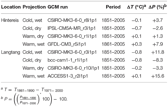
Table 1. Selected ensemble of historical GCM runs for the Hintereisferner and Langtang glaciers with simulated basin-averaged changes in mean temperature and precipitation in 1861–1890 relative to 1971–2000.

The selected models are statistically downscaled using the meteorological data of the Kyangjin and Vent stations by applying a Quantile Mapping methodology that performs well for mountainous terrains (Themeßl et al., 2011). This method is applied by constructing monthly empirical cumulative distribution functions that are calculated for the meteorological data and the historical GCM runs. This encompasses the period 1988–2005 for the Kyangjin station and 1987–2005 for the Vent station. The empirical cumulative distribution functions of the meteorological data and the historical GCM runs are used to calculate correction factors that are subsequently used to bias-correct the historical GCM runs spanning 1851–2005 at a daily time step. The bias-corrected GCM runs are subsequently spatially distributed by using the same temperature and precipitation lapse rates and normalized precipitation fields that are used for the spatial distribution of the meteorological data.

To separately assess the effects of anthropogenic climate change on glacier mass balance and dynamics, we follow two different scenarios: FULL (i.e., combined anthropogenic and natural climate change) and NATURAL (i.e., natural climate change only). The FULL scenario follows climate change simulations according to the outputs of the selected GCMs. To follow the NATURAL scenario, an approach is used that deviates from the CMIP5 approach, which uses climate models that are realizations of the historicalNat experiment, i.e., forced with natural climate forcings only. A different approach is used due to uncertainties that might be introduced by the downscaling of climate change simulations of the historicalNat experiment and by the inconsistencies in the simulated temperature trends that may rise between climate models from the historical experiment and historicalNat experiment. In this study, the NATURAL scenario follows climate change simulations that consist of two parts. The first covers the period 1851–1980 and is identical to the historical GCM runs. The second covers the period 1971–2016 and repeats the historical GCM runs that span the period 1925–1970. By means of this approach we remove the trend in historical climate change simulations after 1970. There is evidence that the anthropogenic climate signal has become a prevailing explanation for the observed decrease in glacier mass since the 1980s (Marzeion et al., 2014; Hirabayashi et al., 2016). Furthermore, the temperature shows stronger increases since the late 1970s and early 1980s (Hartmann et al., 2013; Figure 3). For this reason, we choose to remove the trend in historical climate change simulations after 1970 and to retain the statistics of 1925–1970 in order to cover the second part of the climate change simulations that represent the NATURAL scenario.

Glacier Mass Balance and Ice-Flow Model

We use a spatially-distributed coupled glacier mass balance and ice-flow model to simulate the glacier response under historical climate change. The mass balance model is based on a glacier model developed by Immerzeel et al. (2012) and further refined by Immerzeel et al. (2013) and Shea et al. (2015). The model is set up at a spatial resolution of ~30 × 30 m and runs on a daily time step.

Daily accumulation is assumed to be equal to the total precipitation when the daily air temperature is below a critical threshold temperature. Daily melt (ablation) is simulated by a degree-day approach that distinguishes the effects of aspect and occurs when the daily air temperature is above a critical threshold temperature (Konz and Seibert, 2010; Immerzeel et al., 2012):

$\begin{array}{ll}\mathit{M}=\mathit{D}\mathit{D}{\mathit{F}}_{\mathit{M}}\mathbf{\ast }(\mathit{T}-{\mathit{T}}_{\mathit{c}}):\mathit{f}\mathit{o}\mathit{r}\mathit{T}>{\mathit{T}}_{\mathit{c}}& (1)\end{array}$

where M (mm d⁻¹) is the amount of melt, T (°C) is the daily air temperature, T_c (°C) is the critical threshold temperature, and DDF_M is the modified degree-day factor. The modified degree-day factor is calculated as (Immerzeel et al., 2012):

$\begin{array}{ll}\mathit{D}\mathit{D}{\mathit{F}}_{\mathit{M}}=\mathit{D}\mathit{D}\mathit{F}(1-{\mathit{R}}_{\exp }\mathbf{\text{cos}}\theta )& (2)\end{array}$

where DDF is the degree-day factor (mm°C⁻¹ d⁻¹) and R_exp is a factor that quantifies the aspect (θ) dependence of the degree-day factor. For debris-covered glaciers, an elevation-dependent melt factor, R_debris, is applied to account for the effect of the debris thickness on melt rates, where the magnitude of melt rates generally decreases with increasing debris thickness. The debris melt factors are derived for 50 m elevation bands by using a relative relation between the mean debris thickness in each elevation band and ablation rates (Østrem, 1959). The debris thickness is estimated by an exponential relation between debris thickness and surface temperature, using surface temperature grids that are derived from the TIR band 10 of the Landsat 8 composite and are corrected for emissivity using the ASTER global emissivity product (Kraaijenbrink et al., 2017). It is assumed that the debris thickness and debris melt factors remain constant over time. The effects of supraglacial ponds and ice-cliffs on melt rates are not considered explicitly.

In addition to precipitation, avalanches also contribute significantly to glacier accumulation in steep mountain terrain (Scherler et al., 2011; Ragettli et al., 2015; Shea et al., 2015; Laha et al., 2017). To simulate avalanching, the gravitational snow transport module SnowSlide (Bernhardt and Schulz, 2010) is used, which assumes snow to be transported downslope when a maximum snow-holding depth and a threshold slope of 25° are exceeded (Bernhardt and Schulz, 2010). The maximum snow-holding depth is deep for flat areas, decreases exponentially with increasing slope angle, and is calculated by an exponential regression function (Bernhardt and Schulz, 2010; Ragettli et al., 2015; Stigter et al., 2017):

$\begin{array}{ll}{SWE}_{max}={SS}_1*e^{-{SS}_2*\mathit{S}}& (3)\end{array}$

where SWE_max (m w.e.) is the maximum snow water equivalent, SS₁ (m) and SS₂ (-) are calibrated empirical coefficients, and S (°) is the slope angle. We assume that avalanching does not occur on pixels classified as glaciers. Hence, on slopes steeper than the threshold slope for avalanching (i.e., 25°), all snow water equivalent values of more than 0.5 m are identified as glaciers and the avalanching of this material is disabled.

In the original model of Immerzeel et al. (2012) glacier movement is simulated by Weertman's sliding law. This approach assumes that glaciers flow as ice slides over the bedrock. Although this simplistic approach may be reasonable to represent glacier flow in a regional-scale gridded hydrological model, it certainly does not capture the essence of glacier flow: a combination of basal sliding and internal deformation (Cuffey and Paterson, 2010). Here, we model glacier flow based on SIA in which the ice surface velocity is governed by the local ice thickness and surface slopes. Unlike existing flow-line models (Huss et al., 2007; Adhikari and Huybrechts, 2009; Banerjee and Shankar, 2013), we allow ice to flow on a regular gridded mesh in its preferred direction. This requires us to define the depth-averaged velocity in x and y direction independently as follows (Le Meur et al., 2004):

$\begin{array}{ll}({\mathit{u}}_{\mathit{x}}(\mathit{s}),{\mathit{u}}_{\mathit{y}}(\mathit{s}))=\frac{\mathit{2}\mathit{A}{(\mathit{C}\mathbf{\text{ρ}}\mathit{g})}^{\mathit{n}}}{n+1}|{\nabla }_{\mathit{x}\mathit{y}}\mathit{s}{|}^{\mathit{n}-1}\left(\frac{\partial \mathit{s}}{\partial \mathit{x}},\frac{\partial \mathit{s}}{\partial \mathit{y}}\right){\mathit{h}}^{\mathit{n}+1}& (4)\end{array}$

Note that ${\lceil {\nabla }_{xy}s\rceil }^{n-1}$ assumes that viscosity is isotropic. In the above equation, u_x (s) and u_y (s) (m d⁻¹) are horizontal depth-averaged velocity components in two dimensions as a function of the surface elevation s (m) , A (Pa⁻³ s⁻¹) is the temperature-dependent Glen's flow-law rate constant (Glen, 1955), n = 3 is Glen's flow-law exponent, ρ (kg m⁻³) is the ice density (916.7 kg m⁻³), g (m s⁻²) is the gravitational acceleration, and h (m) is the ice thickness. Equation 4 has been modified by the implementation of a correction factor C. This correction factor modifies the gravitational driving stress by accounting for higher-order physics that are not captured in the SIA model, such as resistances to ice flow due to longitudinal and lateral stress gradients, and basal sliding (Nye, 1965; Farinotti et al., 2009; Adhikari and Marshall, 2011, 2012b). The gravitational driving stress τ_z in two horizontal dimensions is described by Le Meur et al. (2004):

$\begin{array}{ll}({\tau }_{xz},{\tau }_{yz})=\rho g(\mathit{z}-\mathit{s})\left(\frac{\partial \mathit{s}}{\partial \mathit{x}},\frac{\partial \mathit{s}}{\partial \mathit{y}}\right)& (5)\end{array}$

where z (m) represents the depth of a glacier. By modifying the gravitational driving stress with the correction factor C the equation becomes:

$\begin{array}{ll}({\tau }_{xz},{\tau }_{yz})=C\rho g(\mathit{z}-\mathit{s})\left(\frac{\partial \mathit{s}}{\partial \mathit{x}},\frac{\partial \mathit{s}}{\partial \mathit{y}}\right)& (6)\end{array}$

According to Le Meur et al. (2004) equation 5 is eventually used to derive an equation that describes the change in velocity over depth z:

$\begin{array}{ll}\frac{\partial {\text{u}}_x,\partial {\mathit{u}}_y}{\partial z}=-2\mathit{A}{(\text{ρ}\mathit{g})}^{\text{n}}{(\mathit{s}-\mathbf{\text{z}})}^{\text{n}}{\lceil \nabla \mathit{s}\rceil }^{\mathit{n}-1}\left(\frac{\partial \mathit{s}}{\partial \mathit{x}},\frac{\partial \mathit{s}}{\partial \mathit{y}}\right)& (7)\end{array}$

Implementing the correction factor C it results in:

$\begin{array}{ll}\frac{\partial {\mathit{u}}_x,\partial {\mathit{u}}_y}{\partial z}=-2\mathit{A}{(\mathit{C}\mathbf{\text{ρ}}\mathit{g})}^{\mathit{n}}{(\mathit{s}-\mathit{z})}^{\mathit{n}}{\lceil \nabla \mathit{s}\rceil }^{\mathit{n}-1}\left(\frac{\partial \mathit{s}}{\partial \mathit{x}},\frac{\partial \mathit{s}}{\partial \mathit{y}}\right)& (8)\end{array}$

Eventually the integration of equation 8 from z = B (bedrock elevation) to z = s (surface elevation) leads to the formulation of equation 4, where h = s–B.

Mass conservation is ensured by a mass transport equation that relates ice thickness changes to the horizontal flux divergence and changes in the net surface mass balance (e.g., Oerlemans et al., 1998; Adhikari and Huybrechts, 2009; Cuffey and Paterson, 2010):

$\begin{array}{ll}\frac{\partial \mathit{h}}{\partial \mathit{t}}=\mathit{M}-{\nabla }_{\mathit{x}\mathit{y}}\mathit{q}& (9)\end{array}$

where M is the net surface mass balance (m w.e.) and (q_x, q_y) = (u_x(s)h, u_y(s)h) are the horizontal ice fluxes (m² d⁻¹). Equation 4 and 9 are implemented for each grid cell in the model by means of a (centered) finite difference scheme. The finite difference scheme is applied on a regular gridded mesh with a horizontal grid spacing of ~30 m. Furthermore, a forward explicit time stepping scheme with a daily step is used, which is found to be stable.

Model Initialization

To initialize the model, the ice thickness for the Hintereisferner and Langtang Glacier in 1850 is reconstructed.

Hintereisferner

The initial ice thickness for the Hintereisferner is reconstructed using glacier outlines obtained from the Austrian glacier inventories of 1850 and 2006 (Abermann et al., 2009; Fischer et al., 2015), recent (EU-DEM) and reconstructed (1850) DEMs of the glacier surface, and observed ice thickness profiles over the period 1855–2006 that are extracted from Schlosser (1997) and Kuhn (2008). The reconstruction of the initial ice thickness consists of four steps. First, the ice thickness of 2006 and the bed elevation is estimated by the GlabTop2 approach (Frey et al., 2014) using the 2006 outline and the recent surface DEM. Second, average mass balance changes between 1850 and 2006 are derived from the observed ice thickness profiles for 100 m elevation zones. Combined with the recent surface DEM and the 1850 outline, the average mass balance changes are used to derive a first temporary ice thickness map. Third, a surface DEM for 1850 is constructed by inverse distanced weighted interpolation of the 1850 outline elevation. The 1850 surface DEM and the bed elevations are used to derive a second temporary ice thickness map. The final 1850 ice thickness map is the maximum thickness of both temporary maps.

Langtang Glacier

For the Langtang Glacier, observations of ice thickness profiles are not available. For this reason, a different approach is followed to reconstruct the initial ice thickness for 1850. The initial ice thickness is reconstructed by using recent glacier outlines obtained from the Randolph Glacier Inventory (RGI) v6 (Pfeffer et al., 2014), reconstructed glacier outlines (1850), and recent (SRTM) and reconstructed (1850) DEMs of the glacier surface. The reconstruction of the initial ice thickness consists of four steps as well. First, the present ice thickness and bed elevation are estimated by the GlabTop2 approach (Frey et al., 2014) using recent glacier outlines and a recent surface DEM. Second, a first temporary ice thickness map is derived by using the GlabTop2 approach (Frey et al., 2014) in combination with glacier outlines and a surface DEM for 1850. The glacier outlines for 1850 are reconstructed based on the LIA moraines that are derived from Landsat 8 imagery (Roy et al., 2014). Subsequently, the 1850 surface DEM is constructed by inverse distance weighted interpolation of the 1850 lateral moraine elevation. Finally, the 1850 surface DEM and the bed elevations are used to calculate a second temporary ice thickness map. The final 1850 ice thickness map is the maximum thickness of both temporary maps. Due to the lack of knowledge of the 1850 debris extent on Langtang Glacier, we assumed the initial debris extent to be similar to the present-day debris extent (Kraaijenbrink et al., 2017), but extended it laterally (and longitudinal at the terminus) to cover the larger footprint of the glacier in 1850.

Model Calibration and Validation

We use the Parameter ESTimation (PEST) algorithm (Doherty, 2018) to calibrate the model. The model is calibrated in a three-step approach. First, we run the model manually from 1851 to 2005 for each GCM that follows the FULL scenario by applying several iterations. The simulated ice thickness and glacier extents at the end of each run are compared to the current glacier extents and ice thickness, i.e., the outlines and ice thickness of the RGI and 2006 for the Langtang Glacier and Hintereisferner, respectively. The model results from the single GCM runs that, eventually, correspond best to the current outlines and ice thickness are used as initialization for the model calibration runs. These are the cold-wet (Langtang Glacier) and cold-dry (Hintereisferner) GCM-glacier model combinations. Secondly, the model is calibrated on zonal-averaged observed glacier surface velocities and mean glacier surface elevation changes that are estimated over 50-m elevation zones (see below for details). The model is run from 2006 to 2016 and seven parameters are calibrated that influence glacier dynamics and mass balance: the degree day factors for clean-ice (DDF_C) and snow (DDF_S), the critical threshold temperature (T_c), the Glen's flow rate factor (A), the correction factor that accounts for resistances to ice flow due to lateral and longitudinal stress gradients, and basal sliding (C), and the empirical coefficients SS₁ and SS₂. The model is calibrated on the main trunks of Langtang Glacier and Hintereisferner. Finally, several model parameters (see Table 2) and debris melt factors (i.e., R_debris) are manually optimized to improve the long-term model performance. The manual optimization is necessary since the PEST algorithm is not able to optimize the debris melt factors and some of the model parameters (Table 2). To evaluate the model performance, the coefficient of determination (R²) and correlation (R) are used as main efficiency criteria, where the coefficients represent the overall standardized performance of the model in simulating both surface velocities and elevation changes. Additionally, the performance is evaluated on the simulation of surface velocities and elevation changes separately by using the Mean Absolute Error (MAE) as criterium.

TABLE 2

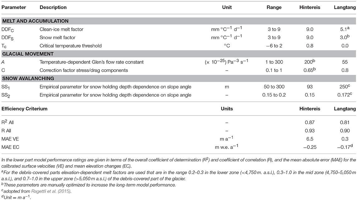
Table 2. Calibrated model parameters, their calibration ranges, and their calibrated values.

The zonal-averaged observed glacier velocities are calculated using COSI-Corr (Co-registration of Optically Sensed Images and Correlation) (Leprince et al., 2007). For Hintereisferner, we derived velocities over the period 2016–2018 using PLANET VNIR bands with an initial window of 128 × 128 pixels (px), a final window of 8 × 8 px, and a step size of 4 px. For Langtang Glacier, velocities are derived over the period 2010–2012, using ASTER VNIR band 2 with an initial window of 64 × 64 px, a final window of 16 × 16 px, and a step size of 4 px. The calculated glacier velocities are subsequently averaged over 50 m elevation zones, which are then used for the calibration of glacier surface velocities. The calibration on zonal-averaged glacier surface elevation changes on Langtang Glacier (over 2006–2014) and Hintereisferner (over 2006–2011) is conducted by using mean annual surface elevation change grids of Langtang Glacier and Hintereisferner that are calculated by means of DEM differencing. We refer to Ragettli et al. (2016) and Klug et al. (2018) for more detailed descriptions on the DEM differencing and the calculation of mean surface elevation changes on Langtang Glacier and Hintereisferner, respectively. The mean surface elevation changes are subsequently averaged over 50 m elevation zones, which are then used for model calibration.

The best performing parameter sets are used to run the model from 1851 till 2016 by using the modeled (1851–2005) and observed (2006–2016) climate data, and to validate the calibrated model on glacier area changes and ice thickness. To reveal the anthropogenic influence on the response of glaciers the model results for the FULL and NATURAL scenarios are compared with each other. The comparison is done for the period 1971–2016 and is conducted by using the outcomes of GCM-glacier model combinations that generate outcomes in close agreement with the observed changes in the glacier mass balance and flow.

Sensitivity Analysis

To gain an improved insight on the sensitivity of surface velocities and elevation changes to model parameter changes, a local One-At-A-Time (OAT) sensitivity analysis (Pianosi et al., 2016) is performed using the SENSAN sensitivity analyser of the PEST algorithm (Doherty, 2018). The analysis is done by varying values of calibration parameters (DDF_C, DDF_S, T_c, A, C, SS₁, and SS₂) independently within ranges that are listed in Table 2 but does not account for parameter interactions. To conduct the analysis, surface velocities and elevation changes are averaged over the calibration period (2006–2016) and the main trunks of Langtang Glacier and Hintereisferner. The sensitivity of these variables are measured by the average linear sensitivity index (ALS) of Nearing et al. (1989):

$\begin{array}{ll}\mathit{A}\mathit{L}\mathit{S}=\frac{\left[\frac{y_2-y_1}{y}\right]}{\left[\frac{x_2-x_1}{x}\right]}& (10)\end{array}$

where y₂ and y₁ represent the output values (y) obtained for the maximum (x₂) and minimum (x₁) of the input parameter ranges (x) (Table 2). x and y represent the means of the parameter values (x₁ and x₂) and respective output values (y₁ and y₂).

Results

Model Calibration and Validation

The best performing parameter sets that result from the calibration approach are listed in Table 2. The parameters associated with melt and accumulation (DDF_C, DDF_S, and T_c) agree well with those observed/modeled in other studies (Hock, 2003; Konz and Seibert, 2010; Lambrecht et al., 2011; Immerzeel et al., 2013). However, the calibrated degree-day factor for snow at the Hintereisferner (i.e., 9 mm°C⁻¹ d⁻¹) is higher than the snow degree-day factors observed/modeled in most studies (i.e., 3–6 mm°C ⁻¹ d⁻¹) (Braithwaite and Zhang, 2000; Singh et al., 2000; Hock, 2003). A potential explanation is the absence of sublimation in the model that can amount to 150 mm yr⁻¹ at Hintereisferner (Kaser, 1983). This might cause mass balance changes to be corrected by a higher snow degree-day factor. The Glen's flow rate constant (A) calibrated for Langtang Glacier is in range of values typical for temperate glaciers (Cuffey and Paterson, 2010). Also, the correction factor (C) of 0.8 falls within the expected range [i.e., 0.45–0.85, based on the study of Farinotti et al. (2009)]. The same applies for the C factor of 0.65 calibrated for Hintereisferner. However, the calibrated Glen's flow rate constant for the Hintereisferner is high and falls outside the expected range. There are several factors that may contribute to the high Glen's flow rate constant as it is affected by factors that are related to the ice rheology of the glacier, such as temperature, density, and water content (Cuffey and Paterson, 2010), and vary widely in space and time. The parameters associated with snow avalanching (SS₁ and SS₂) in the Langtang area are adopted from former studies conducted in the region (Ragettli et al., 2015). The parameters for the Hintereisferner are difficult to compare since no studies have been conducted before in the region using the SnowSlide algorithm. However, the parameters are similar with those in the study of Shea et al. (2015). The debris melt factors are lowest at the lower reaches of the Langtang Glacier due to the presence of thick debris, and highest in the central and upper reaches of the debris-covered part of Langtang Glacier. The high debris melt factors can most likely be explained by thinner debris layers, which cause a smaller reduction of melt rates, and the higher number of supraglacial ponds and ice cliffs in the central domain of the glacier that locally enhance melt (Ragettli et al., 2016; Steiner et al., in press). An alternative explanation for the high debris melt factors are reduced emergence velocities, which also have been found to contribute to increased thinning on debris-covered glaciers (Brun et al., 2018).

Figure 2 shows the simulated and observed surface velocities and elevation changes for Langtang Glacier and Hintereisferner. The best overall model performance is achieved for Hintereisferner (R² = 0.87; Table 2). The mean (minimum/maximum) elevation change is −1.53 (−6.36/+3.73) m w.e. a⁻¹, which is larger than the mean (minimum/maximum) observed elevation change of −1.32 (−6.50/+1.87) m w.e. a⁻¹ (Table 3). The differences between simulated and observed elevation changes can most likely be attributed to local avalanches; at the western margin of the main trunk the maximum and mean simulated positive elevation changes are higher than the observed elevation changes. The largest differences can be found between the observed and simulated velocities with a zonal MAE of 6.5 m a⁻¹ (Table 2), where the mean (minimum/maximum) simulated velocity is 6 (0/26) m a⁻¹ and the mean (minimum/maximum) observed velocity is 12 (0/27) m a⁻¹. The large differences can mainly be explained by the presence of large distortions in the upper part of the glacier that are found in the satellite-derived velocities and reduces the reliability of the observed values. Nevertheless, the modeled velocities are comparable with observed velocities at stone line 6 (i.e., at this location ice flow velocities are measured in situ by using the annual motion of stones placed on the ice surface as a proxy) (Figure 2, Span et al., 1997). The model simulates velocities of 3.2 m a⁻¹ in 2016, which is close to the observed velocities of about 4 m a⁻¹ (Stocker-Waldhuber et al., 2019). The maximum ice thickness of 215 m simulated at the end of 2006 is comparable with the ice thickness estimated with GlabTop2 (220 m). Furthermore, the model can simulate glacier area changes that are in reasonable agreement with the observed ones. The model simulates a glacier area reduction of about 0.5 km² over the period 2006–2011, whereas the observations indicate a reduction of about 0.6 km² (Charalampidis et al., 2018; Klug et al., 2018).

TABLE 3

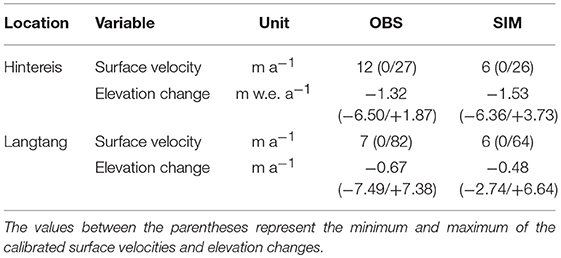
Table 3. Simulated and observed mean surface velocities and elevation changes per glacier tongue.

FIGURE 2

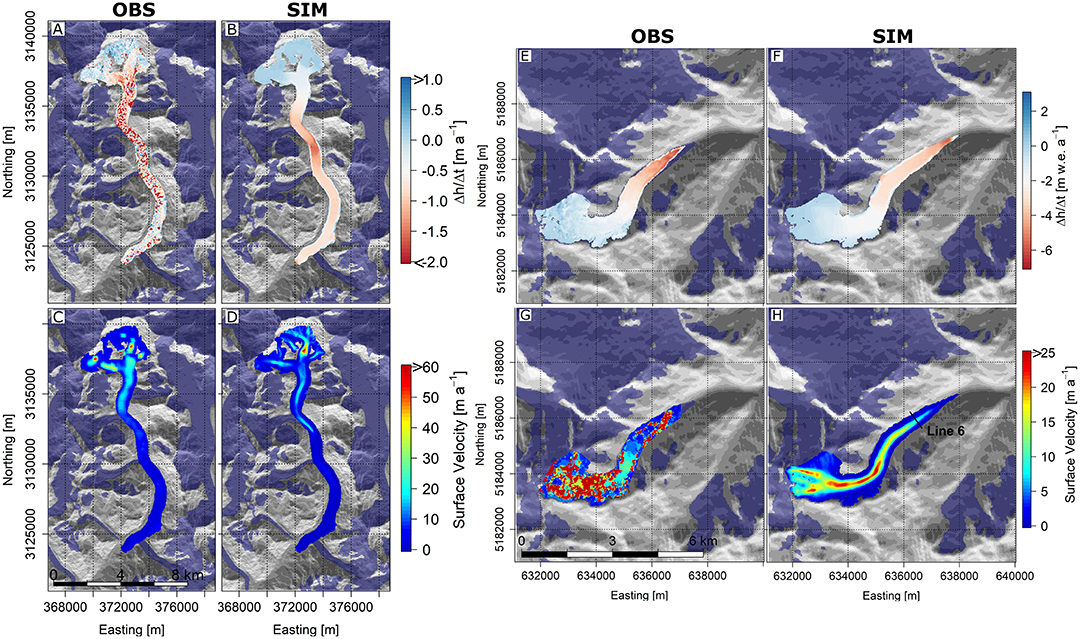
Figure 2. Observed (OBS) and simulated (SIM) mean surface elevation change (A,B,E,F) and velocities (C,D,G,H) for the Langtang (A–D) and Hintereisferner (E–H) glaciers. Line 6 indicates the location of stone line 6 (Span et al., 1997). Source of the observed mean surface elevation change grids are Ragettli et al. (2016) for the Langtang Glacier and Klug et al. (2018) for the Hintereisferner.

The overall fit between the observations and calibrated outcomes (R² = 0.81) is satisfactory for Langtang Glacier as well. The mean (minimum/maximum) elevation change is −0.48 (−2.74/+6.64) m a⁻¹, which is lower than the mean (minimum/maximum) observed elevation change of −0.67 (−7.49/+7.38) m a⁻¹. The largest elevation changes are simulated in the central reaches of the main trunk (4800–5100 m a.s.l.). The high elevation changes can primarily be explained by the higher debris melt factors in this part of the glacier that are due to the presence of melt-enhancing ice cliffs and supraglacial ponds. The model is, however, not able to represent the spatial distribution of ice cliffs and supraglacial ponds sufficiently, which can explain the underestimation of the modeled mean elevation change. The simulated positive elevation changes are largest at the glacier head, i.e., in the accumulation zone, and along the margins of the tongue. The positive elevation changes along the margins can mainly be attributed to avalanching, which is especially large at the eastern side of the main trunk due to the steep side walls generating more avalanches. The observed and modeled velocities are comparable with each other with mean (minimum/maximum) values of 7 (0/82) m a⁻¹ and 6 (0/64) m a⁻¹, respectively. The maximum ice thickness of about 280 m simulated at the end of 2001 (i.e., year of RGI glacier outline) is comparable with the ice thickness estimated with GlabTop2 (290 m), where the maximum ice thickness is simulated in the upper reaches of the main trunk. Further, the modeled glacier area changes between 2006 and 2015 are with 0.55 km² in reasonable agreement with the observed glacier area decline of 0.45 km² (Ragettli et al., 2016).

Model Sensitivity

Table 4 lists the sensitivity of surface velocities and elevation changes to model parameter changes. The modeled velocities are most sensitive to changes in the correction factor C followed by Glen's flow rate constant A. Modeled elevation changes are most sensitive to changes in DDF_C, where Langtang Glacier tends to be less sensitive to changes in DDF_C than the Hintereisferner. The lower sensitivity can most likely be explained by the presence of a thick debris layer at Langtang Glacier that reduces ice melt. Further, modeled velocities and elevation changes are more sensitive for changes in the snow avalanching parameters SS₁ and SS₂ than on the Hintereisferner. The higher sensitivity can most likely be explained by the larger contributions of snow avalanching to accumulation at Langtang Glacier.

TABLE 4

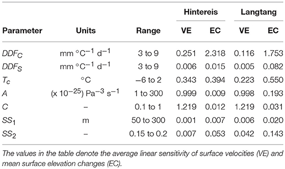
Table 4. Model parameters and parameter ranges used for the sensitivity analysis.

Past Climate Forcing

Since the end of the LIA, both precipitation and temperature have changed in magnitude and distribution. Figure 3 shows the 10-years moving average of daily air temperature and precipitation at the Kyangjin and Vent stations for the FULL and NATURAL scenarios over the past 166 years, i.e., 1851–2016. The precipitation has decreased by 5% (range: −7 to −1%) for FULL and 2% (−3 to −1%) for NATURAL between 1861–1890 and 1981–2010 at Vent station. At Kyangjin station the decreases are a bit larger with relative changes of 6 and 5% for FULL and NATURAL (−18 to +3% for FULL and −11 to +3% for NATURAL), respectively. At the same station the temperature has increased with 0.8°C (range: −0.1 to +1.3°C) for FULL and 0.3°C (−0.3 to +0.6°C) for NATURAL between 1861–1890 and 1981–2010. At Vent station the temperature has increased with 0.6°C (−0.1 to +1.3°C) for FULL and 0.2°C for NATURAL (−0.1 to +0.7°C). The NATURAL scenario shows a decline in temperature after 2000 at the Kyangjin and Vent stations, which is equivalent to the decline in temperature that is simulated by the climate models between the mid 1950s and 1970. This equivalence can be explained by the preservation of the statistics for the period 1925–1970 after 1970. The spread in model hindcasts for precipitation is highly variable in time at both stations, whereas the model spread for temperature shows a clear diverging pattern with the largest spread at the end of the LIA and the smallest at present. For the NATURAL scenario, the model spread after 1970 is equal to the model spread prior to 1970, since the statistics for the period 1925–1970 have been retained.

FIGURE 3

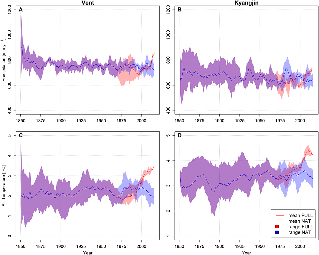
Figure 3. 10-yrs moving averages of simulated precipitation (A,B) and temperature (C,D) changes for the period 1971–2016 for FULL (red) and NATURAL (blue). The moving averages are given for the Vent (A,C) and Kyangjin (B,D) stations. The colored bands denote the range of the simulations.

Glacier Evolution and Dynamics

Figure 4 shows the change in the glacier areas, volumes, and specific mass balance of the Langtang Glacier and Hintereisferner between 1850 and 2016 for the different climate models. At Langtang Glacier, the largest area and volume reductions are simulated under warm climate conditions with an area (volume) reduction from about 60 km² (5.5 km³) in 1850 to about 39 km² (2.0 km³) in 2016. For cold climate conditions the model shows a smaller decline in area (volume) from 60 km² (5.5 km³) to about 50 km² (3 km³). Under both cold/dry and cold/wet climate conditions the modeled extent is in close agreement with the observed extent in 1974 (53.5 km²; Pellicciotti et al., 2015). The modeled extent under cold/dry conditions is in closest agreement with the observed extent in 2006 (46.5 km²; Ragettli et al., 2016) compared to the modeled extents under other climate conditions. Under cold climate conditions, the model following a wet climate scenario shows a slightly smaller loss in ice mass than the model following a dry climate scenario, which is explained by the differences in precipitation since both models simulate the same temperature trends (Table 1). With a cumulative mass loss of about 40 m w.e. since the end of the LIA, the models following cold climate scenarios show a smaller mass loss than those following warm climate scenarios, which simulate a mass loss up to about 70 m w.e.

FIGURE 4

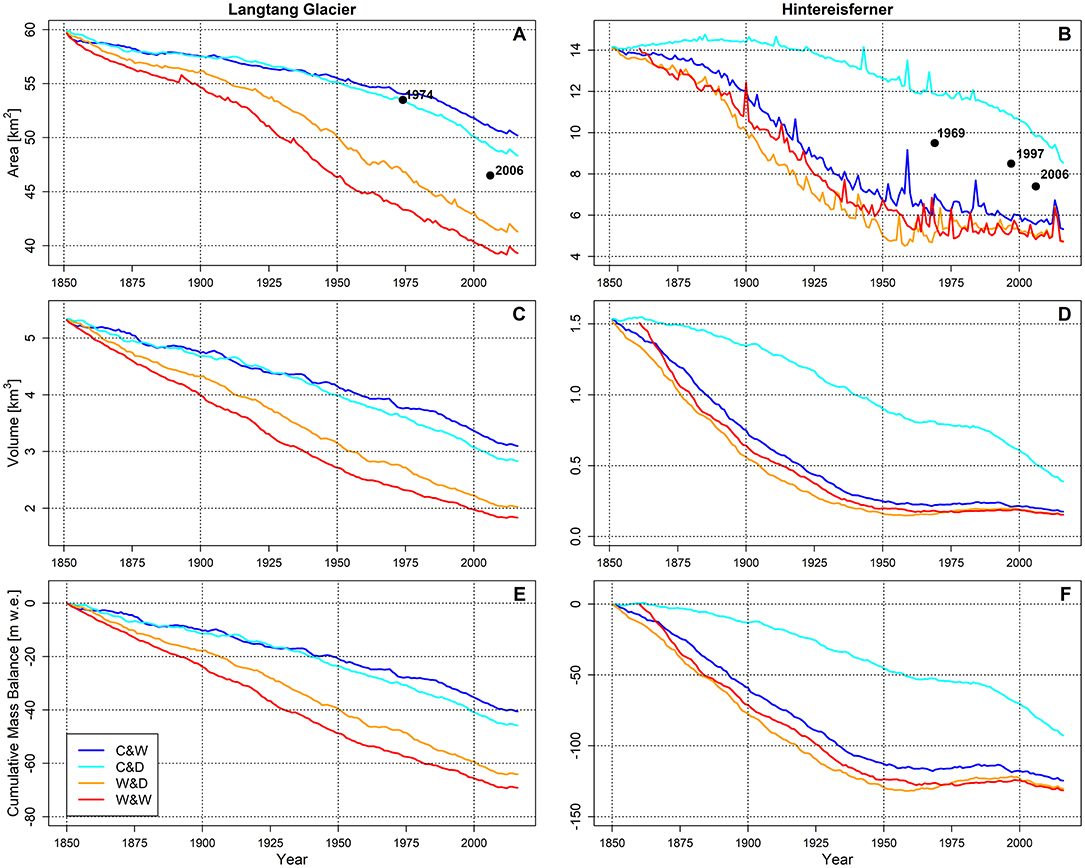
Figure 4. Modeled changes in glacier area (A,B), volume (C,D), and specific mass balance (E,F) of the Langtang Glacier (A,C,E) and Hintereisferner (B,D,F) for four different historical climate change simulations (CW: cold and wet; CD: cold and dry; WW: warm and wet; WD: warm and dry). The black points denote the observed glacier extents at Langtang Glacier (1974, 2016; Pellicciotti et al., 2015; Ragettli et al., 2016) and Hintereisferner (1969, 1997, 2006; Abermann et al., 2009; Patzelt, 2013; Charalampidis et al., 2018).

At Hintereisferner, the largest area (volume) reductions are simulated under warm and cold/wet climate conditions with a decline in area/volume from 14 km² (1.5 km³) up to about 5 km² (0.15 km³), and are accompanied by cumulative mass losses up to about 135 m w.e. Under cold/dry climate conditions, area (volume) reductions are smaller with a decline in area/volume up to about 8 km² (0.4 km³) and a cumulative mass loss up to about 90 m w.e. Under these conditions, extents are simulated that are in closest agreement with the observed extents in 1969 (9.5 km²), 1997 (8.5 km²), and 2006 (7.4 km²) (Abermann et al., 2009; Patzelt, 2013; Charalampidis et al., 2018). All model simulations on the extents show strong inter-annual variability. Since the model reports the ice thickness used for the estimation of extents at the end of the year (i.e., during the winter season), the temporal peaks might be explained by extensive snowfall. This would subsequently cause the threshold value used for the identification of glaciers (0.5 m w.e.) to be exceeded, which explains the short temporal increases in extent. The cumulative mass balance shows a period of reduced mass loss or even a slight mass gain between the 1960s and 1990s, which is commonly known as a period with close-to-balanced climate conditions in the European Alps (Huss, 2012).

Along with changes in the glacier area and volume, surface velocities also change over time. Figure 5 shows transient time series of surface velocity for three different transects along the glaciers. In general, velocity decreases over time at most transects, especially at the main trunks. In the uppermost reaches of Langtang Glacier, velocities are relatively constant after 1875. In the central and lower reaches of the glacier, velocities increase during the late Nineteenth and early Twentieth century, which can most likely be explained by a redistribution of ice mass from the side branches into the main trunk itself. The simulated velocities under cold/wet and warm/dry conditions are with a velocity of about 10 m a⁻¹ in closest agreement with the observed satellite-derived velocities (10 m a⁻¹ for 2010–2012) in the upper domain of the glacier. In central and lower reaches, the simulations deviate from the observations, which can most likely be explained by higher ablation rates that result from neglecting varying surface conditions by the model, e.g., no temporal variation of debris thickness and supraglacial features. Models forced with cold climate models simulate velocities that are in a closer agreement with the observed velocities than the models forced with warmer climate models. In the uppermost reaches of the Hintereisferner, velocities are also relatively constant with exception of the period between the 1960s and 1990s where the velocity time series show a slight increase under warm and cold/wet climate conditions. The slight increases can most likely be explained by the positive mass balance during this period. In the central and lower reaches of the glacier, most simulations show the velocity to become zero due the disappearing glacier in these domains. In the central reaches, the model forced by cold/dry climate change simulations simulates velocities that are comparable with the observed velocities at stone line 6 (Span et al., 1997; Stocker-Waldhuber et al., 2019). The model is however not able to simulate the higher velocities in the 1940s, 1970s, and 1980s, which can most likely be explained by neglecting changing surface or englacial conditions.

FIGURE 5

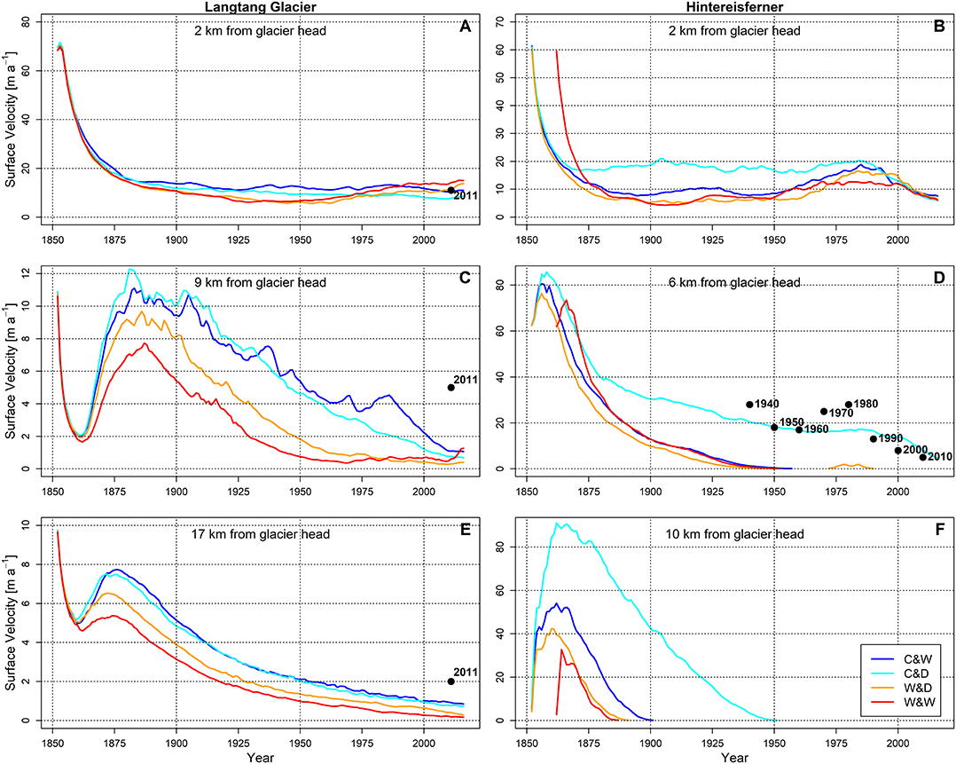
Figure 5. Modeled changes in surface velocity at three different transects along the Langtang Glacier (A,C,E) and Hintereisferner (B,D,F) for four different historical climate change simulations (CW: cold and wet; CD: cold and dry; WW: warm and wet; WD: warm and dry). The locations of the three transects are given in Figure 6. The black points denote the observed velocities at Langtang Glacier (2011) and Hintereisferner (1940, 1950, 1960, 1970, 1980, 1990, 2000; Stocker-Waldhuber et al., 2019).

Figure 6 shows the simulated spatial ice thickness and surface velocity fields for 1850, 1860 (i.e., only for surface velocity) and 2016 under cold/dry and cold/wet conditions, which are selected as conditions that are in closest agreement with the observed changes at Hintereisferner and Langtang Glacier, respectively. At Langtang Glacier the model shows a very limited decrease in length up to about 50 m between 1850 and 2016 (Figure 7), which can mainly be explained by the strong reduction of melt rates due to the presence of thick debris at the lower reaches of the glacier. The limited decrease in length is accompanied by a thinning of the glacier from about 200–300 m (maximum: 355 m) to 100–150 m (maximum: 273 m) under current conditions. An average thinning rate (over 1850–2016) of −0.32 m a⁻¹ and −0.27 m a⁻¹ is estimated for the debris-covered tongue of the glacier and the entire glacier, respectively. These changes are accompanied by decreases in the velocities from up to about 275 m a⁻¹ to 66 m a⁻¹ in the higher parts of the glacier and from about 10–15 m a⁻¹ to about 1–2 m a⁻¹ at the terminus of the glacier. The very low velocities at the terminus of the glacier are typical for the debris-covered Langtang Glacier. Due to enhanced melt in the central reaches of the main trunks (which can be attributed to supraglacial features or reduced emergence velocities) the thinning rate increases, which eventually result in a shallower slope and a stagnation of the terminus. Similar observations have been made in other studies at the Langtang Glacier, and at other debris-covered glaciers in the Central Himalayas as well (Ragettli et al., 2016; Brun et al., 2018; Steiner et al., in press).

FIGURE 6

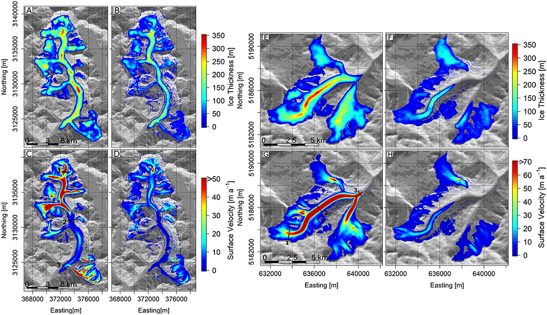
Figure 6. Ice thickness and surface velocity fields of Langtang Glacier (A–D) and Hintereisferner (E–H), showing modeled ice thickness/velocity in 1850/1860 (A,C,E,G) and 2016 (B,D,F,H) for cold/wet (Langtang Glacier) and cold/dry climate conditions (Hintereisferner). The numbers denote the locations of the transects at 2 (2) km, 6 (9) km, and 10 (17) km of the glacier head of Hintereisferner (Langtang Glacier). These transects are used for the modeled velocities given in Figures 5, 8.

FIGURE 7

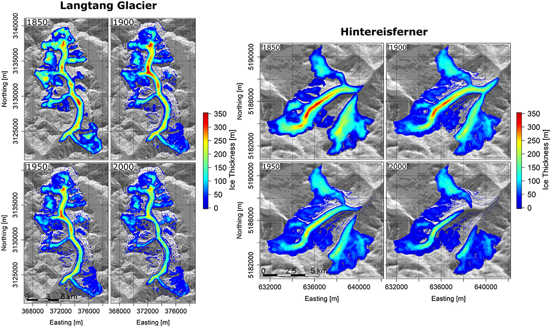
Figure 7. The modeled glacier extents and ice thickness fields of Langtang Glacier (Left) and Hintereisferner (Right) in 1850, 1900, 1950, and 2000 for cold/wet (Langtang Glacier) and cold/dry climate conditions (Hintereisferner).

The Hintereisferner shows a different trend with a significant decrease in length and reduction of ice thickness. The model simulates a decrease in length of about 3 km, which is close to the observed changes in glacier length (e.g., Leclercq and Oerlemans, 2012), and a reduction in ice thickness from about 340 m to about 180 m. Thereby, an average thinning rate (over 1850–2016) of −0.47 m a⁻¹ is estimated for the main trunk of the glacier. Initially the Kesselwandferner and Hintereisferner (Figure 1) were attached to each other, whereas the Hochjochferner was detached. However, the distance between the terminal point of the Hochjochferner and the tongue of the Hintereisferner was with only 50–100 m very short (Blümcke and Hess, 1895). Under cold/dry conditions the model simulates an advance of the Hintereisferner and Hochjochferner in the late Nineteenth and early Twentieth century, which eventually results in a re-connection of the two glaciers (Figure 7). The modeled connection lasts till the 1940s followed by the detachment of the Hintereisferner and Kesselwandferner in the 1980s, which is about six decades later than the observed detachment (Kuhn et al., 1985). This modeled re-connection between the Hochjochferner and Hintereisferner has however never been observed, which can most likely be explained by biases between the climate inputs and the observed climate change, or the limitation of the ice-flow model to simulate changes in the flow characteristics of the glacier. The changes in ice thickness are accompanied by a decline in surface velocities from about 310 m a⁻¹ to about 25 m a⁻¹ at the Hintereisferner. Initially, the highest velocities are simulated at the Hintereisferner. Under current conditions, the model simulates the highest velocities of about 77 m a⁻¹ at the terminus of the Kesselwandferner, which can mainly be attributed to the relatively steep slope (40–45°).

Anthropogenic vs. Natural Influences

Figure 8 shows the changes in glacier area, volume and cumulative mass balance for Langtang Glacier and Hintereisferner under the FULL and NATURAL scenarios between 1971 and 2016. The differences in outcomes between the FULL and NATURAL scenarios are less pronounced for Langtang Glacier. Here, the changes remain negative also under a colder scenario (NATURAL), although the changes are smaller. Only in the late 1980s and early 2010s the glacier mass balance is close to equilibrium. The relative difference in area, volume, and cumulative mass balance between the FULL and NATURAL scenarios is 3, 9, and 40%, respectively, in 2016. At Hintereisferner, glacier area, volume and mass balance decrease initially and are almost balanced after 2000. In 1989, 2005, and 2013, the extent of Hintereisferner shows short temporal increases, which can mainly be explained by extensive snowfall that causes the snow-ice threshold to be exceeded. This phenomenon can also be observed in Figure 4. The relative difference in area, volume, and cumulative mass balance is more pronounced at Hintereisferner with relative differences of 18, 39, and 64%, respectively.

FIGURE 8

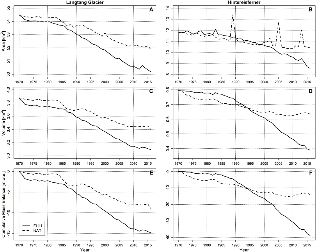
Figure 8. Modeled changes in glacier area (A,B), volume (C,D), and specific mass balance (E,F) of the Langtang Glacier (A,C,E) and Hintereisferner (B,D,F) for the cold/wet (Langtang Glacier) and cold/dry (Hintereisferner) FULL (solid) and NATURAL scenarios (dashed).

The differences in response between Langtang Glacier and Hintereisferner under the FULL and NATURAL scenarios can mainly be explained by differences in the response time. First, the response time of Langtang Glacier is significantly longer than the response time of Hintereisferner. Based on the method of Johannesson et al. (1989), which calculates the response time at the glacier terminus by a ratio between the ice thickness and the mass balance rate, a response time of about 300 years is estimated for Langtang Glacier, whereas Hintereisferner has an estimated response time of about 20 years. These estimates are an indicator for the time a glacier requires to respond to climatic changes. The estimated response times are in the range of those that are found for other debris-covered and clean-ice glaciers (e.g., Shea et al., 2015). The longer response time at Langtang Glacier can most likely be explained by the debris cover that results in a relatively stable terminus position. For this reason, the differences in area, volume, and mass balance are less pronounced between the FULL and NATURAL scenarios. Contrastingly, for Hintereisferner, the differences are pronounced.

The changes in glacier area, volume, and mass balance eventually also influence glacier dynamics. Figure 9 shows the surface velocity time series for two transects in the upper and central reaches of Langtang Glacier and Hintereisferner that are simulated for the FULL and NATURAL scenarios. In the upper reaches of Langtang Glacier, the velocity generally decreases between the late 1980s and late 2000s, and increases during the 1970s, early 1980s, early 1990s, and early 2010s. The increases are most likely due to higher accumulation in the upper reaches of the glacier during these periods. Similar changes are simulated in the upper reaches of Hintereisferner after 1990. In the central reaches, velocity initially decreases, followed by velocities that do not change significantly or show a slight increase. These changes can most likely be explained by higher accumulations compared to the FULL scenario or close to equilibrium conditions that implies the ice thickness does not change and subsequently the velocity does not change either. The velocity changes for Langtang Glacier are smaller than the velocity changes at Hintereisferner. These differences can mainly be explained by the shorter response times at Hintereisferner. The shorter response time causes the glacier to react faster to climatic changes and thinning rates to be higher under a FULL scenario. At Hintereisferner a thinning rate of −0.59 m a⁻¹ is estimated (over 1971–2016) for a FULL scenario relative to an estimated thinning rate of −0.16 m a⁻¹ for a NATURAL scenario, whereas at the debris-covered tongue of Langtang Glacier thinning rates of −0.56 m a⁻¹ and −0.43 m a⁻¹ are estimated for the FULL and NATURAL scenarios, respectively. The higher thinning rates at Hintereisferner lead subsequently to a larger decline in velocity and thus explain the larger changes in velocity. The changing surface velocities and associated changes in thinning rates found at Hintereisferner and Langtang Glacier are in agreement with the recently observed link between glacier flow and thinning rates in High Mountain Asia (Dehecq et al., 2019).

FIGURE 9

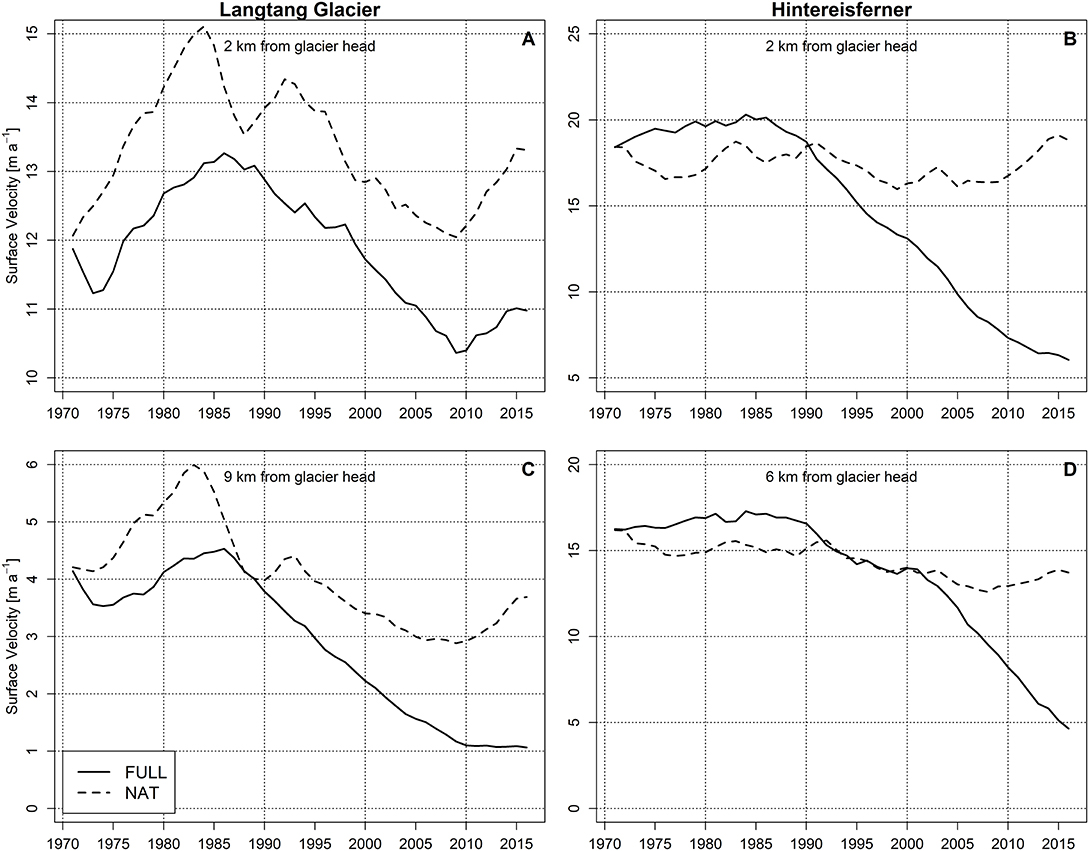
Figure 9. Modeled changes in surface velocity at two different transects along Langtang Glacier (A,C) and Hintereisferner (B,D) for the cold/wet (Langtang Glacier) and cold/dry (Hintereisferner) FULL (solid) and NATURAL scenarios (dashed). The locations of the two transects are given in Figure 6.

The less negative or even close to equilibrium glacier mass balance at Langtang Glacier and Hintereisferner eventually result in larger ice thickness at the end of a model run. Figure 10 shows the ice thickness and velocity fields at the end of a FULL-run and a NATURAL-run. At Langtang Glacier the difference between the maximum ice thickness of 283 m for NATURAL and 273 m for FULL is small. The higher ice thickness leads subsequently to higher flow velocities up to about 87 m a⁻¹. At Hintereisferner the differences in outcomes between the FULL and NATURAL scenarios are larger. Instead of a maximum ice thickness of about 180 m, ice thickness up to about 230 m is simulated for NATURAL. The associated velocities are higher with rates up to about 156 m a⁻¹ at the terminus of the Kesselwandferner. There, the high velocities can mainly be attributed to the relatively steep slope in combination with a larger ice thickness than simulated for the FULL scenario. It can therefore be concluded that human-induced climate change has a significant impact on the mass balance and dynamics of glaciers. The magnitude of impact depends on the response time of the glacier, where a debris-covered glacier such as the Langtang Glacier shows a longer response time than a clean-ice glacier such as the Hintereisferner. It is therefore likely that that human-induced climate change has a larger impact on clean-ice glaciers than on debris-covered glaciers.

FIGURE 10

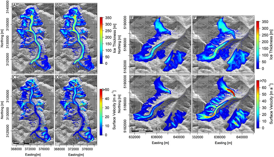
Figure 10. Ice thickness and surface velocity fields of the Langtang Glacier (A–D) and Hintereisferner (E–H), showing modeled ice thickness/velocity in 2016 for the cold/wet (Langtang Glacier) and cold/dry (Hintereisferner) FULL (A,C,E,G) and NATURAL scenarios (B,D,F,H).

Discussion

Uncertainties and Limitations

The outcomes of the glacier mass balance and ice-flow model are subject to several uncertainties and limitations that can be subdivided into three main groups: climate change simulations, the parameterization and representation of physical processes in the model, and the calibration procedure.

To assess the response of glaciers to historical climate change, an ensemble of four distributed and bias-corrected GCMs were used that cover a wide range of possible climate conditions. These models have been selected by means of an advanced envelope-based selection approach based on changes in climatic means and their skill in simulating the local climate. The outputs of the selected climate models are bias-corrected on meteorological data of the Kyangjin and Vent stations and are subsequently spatially distributed by using local monthly temperature lapse rates, normalized seasonal precipitation fields and high-resolution digital elevation models. The lapse rates are assumed to be constant in space and from year-to-year, whereas lapse rates are variable in space and time (Kirchner et al., 2013; Immerzeel et al., 2014; Heynen et al., 2016; Steiner and Pellicciotti, 2016). The lack of interannual and spatial variability might eventually introduce uncertainties in the climate fields, which propagates into the model results. The lack of spatiotemporal variability in lapse rates also introduce long-term uncertainties, especially since glaciers are sensitive to temperature changes that emerge from small changes in temperature lapse rates. Therefore, a correction of lapse rates might be needed to improve the long-term performance of the model. In our study temperature lapse rate corrections resulted in steeper lapse rates with monthly maximum (minimum) lapse rates that amount to 0.0076 (0.0052)°C m⁻¹ in March-April (July) at Langtang Glacier and 0.0086 (0.0049)°C m⁻¹ in March (December) at Hintereisferner. Thereby, the corrected lapse rates at Langtang Glacier fall in range with the lapse rates observed by Heynen et al. (2016). The corrected lapse rates at Hintereisferner are relatively steep compared to lapse rates that are mostly found in the European Alps (Rolland, 2003), but are still comparable with lapse rates found in other parts of the European Alps (Nigrelli et al., 2018). In addition, the limited data availability at higher altitudes hampers the validation of climate fields, especially in areas with difficult accessibility, such as upper Langtang Valley. Techniques, such as dynamical downscaling using high-resolution weather models, might contribute to an improvement of the accuracy and quality of climate fields in the complex mountainous environments of the upper Langtang and Rofental valleys (Bonekamp et al., 2018).

To separately assess the effects of human-induced climate change on the glacier response we followed two scenarios: FULL and NATURAL. The FULL scenario followed climate change simulations according to GCM outputs that follow the historical experiment of the CMIP5 archive, whereas the NATURAL scenario followed climate change simulations that are identical to the FULL scenario (until 1970) and retained the statistics of the climate change simulations prior to 1970 (i.e., 1925–1970). A limitation of retaining the statistics is that temperature trends such as the temperature decline simulated at the Kyangjin and Vent stations between the mid 1950s and 1970 are repeated after 1970, which subsequently introduces uncertainties in the model outcomes. An alternative approach would be to follow climate change simulations of the historicalNat experiment (i.e., GCM experiment forced with natural forcings only). However, the limitation of this approach is that simulations of the historicalNat experiment are difficult to bias-correct which might introduce additional uncertainties. Additionally, the selection approach we followed would allow us to select the same ensemble models and members as the historical experiment. This might have a limitation since the forcing of a historicalNat experiment is different, which in combination with a different parameterization might lead to a trend opposite of what is expected under natural climate conditions, i.e., increasing temperatures relative to a historical experiment instead of constant or decreasing temperatures. Since our aim was to attribute the response of glaciers to anthropogenic and natural climate change, we chose to remove the trend in historical climate change simulations after 1970, which are clearly anthropogenic due to the strong observed human-induced increases in temperature, and to repeat the historical GCM runs spanning the period 1925–1970.

The glacier mass balance and dynamics were simulated by using a coupled glacier mass balance and ice-flow model that is based on a gridded formulation of the shallow ice approximation. One limitation is that sublimation processes are not included in the model, which is a considerable loss term in high mountain environments. For instance, at Hintereisferner sublimation losses of about 150 mm yr⁻¹ have been reported by Kaser (1983). In the Langtang Valley, sublimation losses can amount up to 21% of the total snowfall, and can even be higher at wind-exposed locations (Stigter et al., 2018). The model might correct for these mass losses by adapting degree-day factors to increase the amount of loss by melt, which subsequently might result in overestimation of the calibrated glacier and snow degree-day factors. Another scenario is that snow storage and cover is overestimated, particularly at the high ridges that are prone to wind-blown transport of snow. To account for sublimation techniques are required that do not have a high data demand, but still can give reasonable sublimation estimates. Another limitation might be the use of a simple degree-day approach for the simulation of ice and snowmelt. Gabbi et al. (2014) found in a model comparison study that parameters of a simplified degree-day approaches are not robust in time and require recalibration for different climate conditions. The authors found that models including a separate term for shortwave radiation are able to produce robust simulations of ice and snowmelt. Therefore, these types of models can be seen as a suitable alternative to simplified degree-day approaches. Similar findings were also found by Litt et al. (2019) who tested the performance of (enhanced) temperature-index approaches in the Central Himalayas. The authors found however that these approaches can be underperforming where sublimation or other wind-driven processes contribute to ablation, such as in the accumulation zones. To improve the performance of the simplified degree-day approach applied in this study we distinguish the effect of aspect and include an elevation-dependent melt factor that accounts for the effect of debris thickness on melt rates.

A limitation that also might affect the model outcomes is the way how avalanching is simulated in the model. To simulate avalanching the gravitational snow transport module SnowSlide (Bernhardt and Schulz, 2010) is used. The drawback of this approach is that the module is solely restricted in use to snow avalanching, which disables the possibility to apply the algorithm for pixels that are classified as glacier. This means that on slopes steeper than the threshold slope (i.e., 25°) the avalanching of this material needs to be disabled, achieved in this study by assuming a threshold value that identifies a pixel as a glacier when the snow water equivalent is higher than 0.5 m. Although the model is able to simulate avalanches sufficiently at Langtang Glacier (i.e., especially at the eastern margins with steep side walls; Figure 2), the threshold value might also introduce uncertainties. For instance, the strong interannual variability in glacier area at Hintereisferner can mainly be attributed to the used threshold value. It is, however, difficult to validate the threshold value and the contribution of avalanching to the mass balance of the glaciers due to a lack of reliable snowfall observations. Further improvements in the simulation of avalanching might be achieved by the combination of the SnowSlide module with existing modeling tools, such as the mass-conserving algorithm of Gruber (2007). This algorithm is an extension of flow-routing and terrain parameterization techniques and has the advantage that it can simulate the gravitational transport of other types of movements, such as ice avalanches or debris flows, as well. Further, the algorithm can easily be integrated in glacier mass balance and ice-flow models similar to the one presented here.

Flow velocities are largely dependent on ice rheology and dynamics as well as ice thickness and surface slope. Large unknowns, or processes not considered in the model, likely introduced uncertainties. Large unknowns are for instance the ice thickness changes since the end of the LIA, especially at Langtang Glacier where observations are lacking. Processes that have not been considered in the model are, for instance, the role of crevassing. Crevasses can play a crucial role in the mass balance and dynamics of glaciers by locally enhancing ablation and ice flow velocities (Colgan et al., 2016).

Another limitation is the assumed stationarity of model parameters in the model, which is also recognized as a major limitation in other type of models, such as hydrological models (e.g., Merz et al., 2011; Westra et al., 2014; Wijngaard et al., 2018). For instance, the spatial distribution of supraglacial debris, ponds and cliffs are highly variable over time. The spatio-temporal variability influences melt factors that in the model are assumed to be constant over time, which eventually might result in a local over- or underestimation of melt and subsequently also in an over- or underestimation of flow velocities. In addition, the debris and supraglacial characteristics of Langtang Glacier at the end of the LIA are a large unknown. Another example is the spatio-temporal variability in ice parameters, such as ice density or ice temperature, which influences ice viscosity and subsequently ice dynamics (e.g., Zhang et al., 2013). Since ice flow parameters, such as ice density, the temperature-dependent flow rate parameter A, and the correction factor C are assumed to be stationary, uncertainties might be introduced in the simulated flow velocities. For instance, the assumed stationarity of the correction factor C might be an explanation for the underestimated flow velocities at Hintereisferner during the 1940s, 1970s, and 1980s. To improve the representation of feedbacks between ice temperature and flow velocities, combined modeling approaches including models that simulate the thermodynamical behavior of a glacier would be a future improvement. To improve the spatio-temporal variability of supraglacial debris and thus the amount of melt on the glacier, coupled mass balance and ice-flow models need to be combined with modeling approaches that can simulate the spatio-temporal evolution of supraglacial debris (Naito et al., 2000; Jouvet et al., 2011; Rowan et al., 2015).

The coupled glacier mass balance and ice-flow model is calibrated on observed mean surface elevation changes and surface velocities that are both derived from spaceborne imagery. This can be major advantage in remote areas where mass balance or surface velocity data are limited or not available at all. The limitation, however, is that the use of satellite images is restricted in use to several conditions, such as the absence of clouds and snow. When satellite images are available, the images might be prone to noise or distortions, which, in turn, hampers calibration of the model. Further, uncertainties might have been introduced through the calibration approach. The model parameters have been calibrated using an automatic optimization algorithm followed by a manual optimization. No distinctions have been made in the performance of the model in simulating separate components of the high-mountain cryosphere, such as snow cover. Because of that equifinality problems might have been introduced that affect the amount of melt simulated by the model. To minimize equifinality problems in the future, systematic approaches (Pellicciotti et al., 2012; Lutz et al., 2016a; Wijngaard et al., 2017) are recommended that can calibrate the model in multiple consecutive steps by using the combination of snow cover, mass balance, and surface velocity data.

Shallow Ice Approximation

To assess the response of glaciers under changing climate conditions we apply a coupled glacier mass balance and ice-flow model that is based on a spatially-distributed formulation of the SIA. The main advantage of this approach is that the model does not require a priori information on the flowline geometry, but also has other advantages which are mainly related to the low computational expense and complexity. There is a concern that the SIA becomes deficient for fast-flowing glaciers and steep/narrow glacier since the approach does not account for higher-order physics, such as longitudinal and lateral stress gradients (Le Meur et al., 2004; Adhikari and Marshall, 2013). According to Le Meur et al. (2004) the slope is the most important criterion for the applicability of the SIA, where SIA models can still be considered as acceptable for bedrock slopes smaller than 20%. The mean (minimum/maximum) bedrock slope of Langtang Glacier and Hintereisferner are 44 (0/93%) and 44 (0/81%), respectively, which means from this point of view the SIA approach would be deficient. However, Le Meur et al. (2004) did not include correction factors that account for higher-order physics, which are normally neglected by the SIA approach. Also, the authors did not calibrate the Glen's flow rate constant. In our model correction factors that account for longitudinal and lateral stress gradients are included (Nye, 1965; Adhikari and Marshall, 2011, 2012b). Furthermore, Glen's flow rate constant is calibrated on observed surface velocities. This combination results in valid outcomes, which shows that the SIA approach is even reliably on steeper slopes. For example, at the Kesselwandferner velocities up to 77 m a⁻¹ are simulated where the bedrock slope is ~44%. Although these velocities do not agree with the present-day observed velocities of ~20 m a⁻¹ (i.e., ablation stakes L8, L9, and L10) due to an overestimation of ice thickness, velocities with the same order of magnitude (80–90 m a⁻¹) have been observed in the 1970s/1980s (Stocker-Waldhuber et al., 2019). It illustrates the ability of the model to simulate realistic velocities at steeper slopes. Additionally, the use of correction factors in combination with the SIA approach sustains the simplicity of ice flow models, which makes it suitable for potential application in catchment- or regional scale (cryospheric-)hydrological models.

Conclusions and Outlook

The aim of this study is to develop and apply a spatially distributed coupled glacier mass balance and ice-flow model to attribute the response of two glaciers to anthropogenic and natural climate change. We focus on two glaciers with contrasting surface characteristics: the debris-covered Langtang Glacier in the Central Himalayas, and the clean-ice Hintereisferner in the European Alps. We apply the model from the end of the Little Ice Age (1850) to the present-day (2016) by forcing the model with bias-corrected and distributed GCM runs that represent a wide range of region-specific possible climate conditions. The model outputs are used to analyse the evolution and dynamics of the two glaciers, and subsequently to reveal the anthropogenic influence by comparing outputs of two scenarios: one scenario considering the human-induced rapid increases in temperature after 1970 and one scenario that retains the climate conditions prior to 1970.

The results indicate that the coupled glacier mass balance and ice-flow model, based on a gridded formulation of the shallow ice approximation, performs reasonably well for both clean-ice and debris-covered glaciers.

Both glaciers experience the largest area and volume reductions under warm climate conditions, whereas for cold climate conditions the model show a smaller reduction. In addition, the cold model (i.e., cold/dry for Hintereisferner and cold/wet for Langtang) simulates changes that are close to the observed trends. These models simulate area (volume) reductions of 16 (42%) for the Langtang Glacier and of 40 (75%) for the Hintereisferner between 1850 and 2016. Simultaneously with changes in the extents and volumes, surface velocities generally decrease over time from up to 275 to 66 m a⁻¹ at Langtang Glacier and from up to 310 to 25 m a⁻¹ at Hintereisferner. The simulated changes over time are smaller in magnitude for the Langtang Glacier, which can mainly be attributed to the debris cover that insulates the surface and thus reduces the amount of melt. Additionally, the debris cover maintains the position of the terminus. Instead the glacier thins, which eventually result in a shallower profile and a stagnation of velocities at the terminus of the glacier. At Hintereisferner melt rates are higher and the glacier retreats with about 3 km over length under cold/dry climate conditions.

Simulations show that anthropogenic climate change has been accompanied with a rapid increase in temperature after 1970. This has resulted in a larger decline in area/volume compared to a scenario where the anthropogenic influence is less significant (i.e., NATURAL scenario). At Langtang Glacier, the changes in area, volume, and ice thickness remain negative for the NATURAL scenario. Only in the late 1980s and early 2010s the glacier mass balance is close to equilibrium. The relative area, volume and cumulative mass balance difference between a cold/wet FULL and NATURAL scenario at the end of 1971–2016 is 3, 9, and 40%, respectively. At Hintereisferner the glacier area, volume, and ice thickness decrease initially followed by an almost balanced state after 2000. Here, the relative area, volume and cumulative mass balance difference between a cold/dry FULL and NATURAL scenario at the end of 1971–2016 is 18, 39, and 64%, respectively. The decline in area, volume, and ice thickness are accompanied by changing surface velocities that generally increase or do not change significantly. The difference in the response of glaciers between a FULL and a NATURAL scenario is larger for the Hintereisferner mainly due to shorter response times. The shorter response times cause the glacier to react faster to climatic changes and thinning rates to be larger. The larger thinning rates do subsequently lead to a larger decline in area, volume, cumulative balance, and velocity. The simulated velocity changes and associated changes in thinning rates are in agreement with the recently observed link between glacier flow and thinning rates in High Mountain Asia. For a debris-covered glacier the differences are less pronounced due to a longer response time, which can mainly be attributed to the debris cover that insulates the glacier surface and reduces melt.

The outcomes of this study show that the gridded formulation of the shallow ice approximation performs well and is a suitable alternative for higher order or Stokes approaches, especially while modeling a large-scale ensemble of glaciers. Although improvements are needed in future research, the combination of satellite-based imagery and the use of the gridded formulation of the shallow ice approximation should be explored toward investigating the dynamical response of glaciers and its implications for hydrology at a regional scale.

Author Contributions

The study is designed by RW, SA, AB, and WI. The model was run by RW. The data used for calibration of the data were prepared and provided by JS, PK, and CK. The analyses on the simulation outcomes were performed by RW. RW prepared the paper. The figures were prepared by RW. Finally, the proof reading was performed by all (co-)authors.

Funding

This project has received funding from the European Research Council (ERC) under the European Union's Horizon 2020 research and innovation program (grant agreement No. 676819). This work is part of the research program VIDI with project number 016.161.208, which is (partly) financed by the Netherlands Organization for Scientific Research (NWO).

Conflict of Interest Statement

AL was employed by the company FutureWater.

The remaining authors declare that the research was conducted in the absence of any commercial or financial relationships that could be construed as a potential conflict of interest.

Acknowledgments

We thank Silvan Ragettli for sharing the mean annual surface elevation change grids of Langtang Glacier. We thank Maxime Litt and Sonu Khanal for the helpful discussions. We thank two reviewers and the associate editor for their constructive remarks and suggestions that helped us to improve the manuscript significantly.

References

Aðalgeirsdóttir, G., Guð*mundsson, S., Björnsson, H., Palsson, F., Jóhannesson, T., Hannesdóttir, H., et al. (2011). Modelling the 20th and 21st century evolution of Hoffellsjökull glacier, SE-Vatnajökull, Iceland. Cryosphere 5, 1961–1975. doi: 10.5194/tc-5-961-2011

CrossRef Full Text | Google Scholar

Abermann, J., Lambrecht, A., Fischer, A., and Kuhn, M. (2009). Quantifying changes and trends in glacier area and volume in the Austrian Ötztal Alps (1969-1997-2006). Cryosphere 3, 205–215. doi: 10.5194/tc-3-205-2009

CrossRef Full Text | Google Scholar

Adhikari, S., and Huybrechts, P. (2009). Numerical modelling of historical front variations and the 21st-century evolution of glacier AX010, Nepal Himalaya. Ann. Glaciol. 50, 27–34. doi: 10.3189/172756409789624346

CrossRef Full Text | Google Scholar

Adhikari, S., and Marshall, S. J. (2011). Improvements to shear-deformational models of glacier dynamics through a longitudinal stress factor. J. Glaciol. 57, 1003–1016. doi: 10.3189/002214311798843449

CrossRef Full Text | Google Scholar

Adhikari, S., and Marshall, S. J. (2012a). Glacier volume-area relation for high-order mechanics and transient glacier states. Geophys. Res. Lett. 39:L16505. doi: 10.1029/2012GL052712

CrossRef Full Text | Google Scholar

Adhikari, S., and Marshall, S. J. (2012b). Parameterization of lateral drag in flowline models of glacier dynamics. J. Glaciol. 58, 1119–1132. doi: 10.3189/2012JoG12J018

CrossRef Full Text | Google Scholar

Adhikari, S., and Marshall, S. J. (2013). Influence of high-order mechanics on simulation of glacier response to climate change: insights from Haig Glacier, Canadian Rocky Mountains. Cryosphere 7, 1527–1541. doi: 10.5194/tc-7-1527-2013

CrossRef Full Text | Google Scholar

Adhikari, S., Marshall, S. J., and Huybrechts, P. (2011). On characteristic timescales of glacier AX010 in the Nepalese Himalaya. Bull. Glaciol. Res. 29, 19–29. doi: 10.5331/bgr.29.19

CrossRef Full Text | Google Scholar

Banerjee, A. (2017). Brief communication: thinning of debris-covered and debris-free glaciers in a warming climate. Cryosphere 11, 133–138. doi: 10.5194/tc-11-133-2017

CrossRef Full Text | Google Scholar

Banerjee, A., and Shankar, R. (2013). On the response of Himalayan glaciers to climate change. J. Glaciol. 59, 480–490. doi: 10.3189/2013JoG12J130

CrossRef Full Text | Google Scholar

Beniston, M., Farinotti, D., Stoffel, M., Andreassen, L. M., Coppola, E., Eckert, N., et al. (2018). The European mountain cryosphere: a review of its current state, trends, and future challenges. Cryosphere 12, 759–794. doi: 10.5194/tc-12-759-2018

CrossRef Full Text | Google Scholar

Bernhardt, M., and Schulz, K. (2010). SnowSlide: a simple routine for calculating gravitational snow transport. Geophys. Res. Lett. 37:L11502. doi: 10.1029/2010GL043086

CrossRef Full Text | Google Scholar

Berthier, E., and Vincent, C. (2012). Relative contribution of surface mass-balance and ice-flux changes to the accelerated thinning of Mer de Glace, French Alps, over 1979-2008. J. Glaciol. 58, 501–512. doi: 10.3189/2012JoG11J083

CrossRef Full Text | Google Scholar

Blümcke, A., and Hess, H. (1895). Der Hochjochferner in Jahre 1893. Zeitschrift Dtsch Österreichischen Alpenvereins 26:340. Available online at: https://www.e-rara.ch/zut/content/zoom/11639790

Bonekamp, P. N. J., Collier, E., and Immerzeel, W. W. (2018). The impact of spatial resolution, land use, and spinup time on resolving spatial precipitation patterns in the Himalayas. J. Hydrometeorol. 19, 1565–1581. doi: 10.1175/JHM-D-17-0212.1

CrossRef Full Text | Google Scholar

Braithwaite, R. J., and Zhang, Y. (2000). Sensitivity of mass balance of five Swiss glaciers to temperature changes assessed by tuning a degree-day model. J. Glaciol. 46, 7–14. doi: 10.3189/172756500781833511

CrossRef Full Text | Google Scholar

Brun, F., Wagnon, P., Berthier, E., Shea, J. M., Immerzeel, W. W., Kraaijenbrink, P. D. A., et al. (2018). Ice cliff contribution to the tongue-wide ablation of Changri Nup Glacier, Nepal, central Himalaya. Cryosphere 12, 3439–3457. doi: 10.5194/tc-12-3439-2018

CrossRef Full Text | Google Scholar

Charalampidis, C., Fischer, A., Kuhn, M., Lambrecht, A., Mayer, C., Thomaidis, K., et al. (2018). Mass-budget anomalies and geometry signals of three Austrian glaciers. Front. Earth Sci. 6:218. doi: 10.3389/feart.2018.00218

CrossRef Full Text | Google Scholar

Clarke, G. K. C., Jarosch, A. H., Anslow, F. S., Radić, V., and Menounos, B. (2015). Projected deglaciation of western Canada in the twenty-first century. Nat. Geosci. 8, 372–377. doi: 10.1038/ngeo2407

CrossRef Full Text | Google Scholar

Colgan, W., Rajaram, H., Abdalati, W., McCutchan, C., Mottram, R., Moussavi, M. S., et al. (2016). Glacier crevasses: observations, models, and mass balance implications. Rev. Geophys. 54, 119–161. doi: 10.1002/2015RG000504

CrossRef Full Text | Google Scholar

Collier, E., and Immerzeel, W. W. (2015). High-resolution modeling of atmospheric dynamics in the Nepalese Himalaya. J. Geophys. Res. 120, 9882–9896. doi: 10.1002/2015JD023266

CrossRef Full Text | Google Scholar

Cuffey, K. M., and Paterson, W. S. B. (2010). Physics of Glaciers, Fourth Edition. Amsterdam: Academic Press Inc.

Dee, D. P., Uppala, S. M., Simmons, A. J., Berrisford, P., Poli, P., Kobayashi, S., et al. (2011). The ERA-interim reanalysis: configuration and performance of the data assimilation system. Q. J. R. Meteorol. Soc. 137, 553–597. doi: 10.1002/qj.828

CrossRef Full Text | Google Scholar

Dehecq, A., Gourmelen, N., Gardner, A. S., Brun, F., Goldberg, D., Nienow, P. W., et al. (2019). Twenty-first century glacier slowdown driven by mass loss in high mountain Asia. Nat. Geosci. 12, 22–27. doi: 10.1038/s41561-018-0271-9

CrossRef Full Text | Google Scholar

Doherty, J. (2018). PEST: Model-Independent Parameter Estimation, User Manual: 7th Edition. Brisbane, QLD: Watermark Numerical Company.

EEA (2017). Digital Elevation Model over Europe (EU-DEM). Available online at: https://www.eea.europa.eu/data-and-maps/data/eu-dem (accessed September 26, 2017).

Egholm, D. L., Knudsen, M. F., Clark, C. D., and Lesemann, J. E. (2011). Modeling the flow of glaciers in steep terrains: the integrated second-order shallow ice approximation (iSOSIA). J. Geophys. Res. Earth Surf. 116:F02012. doi: 10.1029/2010JF001900

CrossRef Full Text | Google Scholar

Faillettaz, J., Funk, M., and Vincent, C. (2015). Avalanching glacier instabilities: review on processes and early warning perspectives. Rev. Geophys. 53, 203–224. doi: 10.1002/2014RG000466

CrossRef Full Text | Google Scholar

Farinotti, D., Huss, M., Bauder, A., Funk, M., and Truffer, M. (2009). A method to estimate the ice volume and ice-thickness distribution of alpine glaciers. J. Glaciol. 55, 422–30. doi: 10.3189/002214309788816759

CrossRef Full Text | Google Scholar

Farr, T. G., Rosen, P. A., Caro, E., Crippen, R., Duren, R., Hensley, S., et al. (2007). The shuttle radar topography mission. Rev. Geophys. 45:RG2004. doi: 10.1029/2005RG000183

CrossRef Full Text | Google Scholar

Fischer, A. (2010). Glaciers and climate change: interpretation of 50 years of direct mass balance of Hintereisferner. Glob. Planet. Change 71, 13–26. doi: 10.1016/j.gloplacha.2009.11.014

CrossRef Full Text | Google Scholar

Fischer, A., Seiser, B., Stocker-Waldhuber, M., Mitterer, C., and Abermann, J. (2015). Tracing glacier changes in Austria from the Little Ice Age to the present using a lidar-based high-resolution glacier inventory in Austria. Cryosphere 9, 753–766. doi: 10.5194/tc-9-753-2015

CrossRef Full Text | Google Scholar

Frey, H., Haeberli, W., Linsbauer, A., Huggel, C., and Paul, F. (2010). A multi-level strategy for anticipating future glacier lake formation and associated hazard potentials. Nat. Hazards Earth Syst. Sci. 10, 339–352. doi: 10.5194/nhess-10-339-2010

CrossRef Full Text | Google Scholar

Frey, H., Machguth, H., Huss, M., Huggel, C., Bajracharya, S. R., Bolch, T., et al. (2014). Estimating the volume of glaciers in the Himalayan-Karakoram region using different methods. Cryosphere 8, 2313–2333. doi: 10.5194/tc-8-2313-2014

CrossRef Full Text | Google Scholar

Gabbi, J., Carenzo, M., Pellicciotti, F., Bauder, A., and Funk, M. (2014). A comparison of empirical and physically based glacier surface melt models for long-term simulations of glacier response. J. Glaciol. 60, 1140–1154. doi: 10.3189/2014JoG14J011

CrossRef Full Text | Google Scholar

Glen, J. W. (1955). The creep of polycrystalline ice. Proc. R. Soc. A 228, 519–538. doi: 10.1098/rspa.1955.0066

CrossRef Full Text | Google Scholar

Gregory, J. M., White, N. J., Church, J. A., Bierkens, M. F. P., Box, J. E., Van den Broeke, M. R., et al. (2013). Twentieth-century global-mean sea level rise: is the whole greater than the sum of the parts? J. Clim. 26, 4476–4499. doi: 10.1175/JCLI-D-12-00319.1

CrossRef Full Text | Google Scholar

Greuell, W. (1992). Hintereisferner, Austria: mass-balance reconstruction and numerical modelling of the historical length variations. J. Glaciol. 38, 233–244. doi: 10.1017/S0022143000003646

CrossRef Full Text | Google Scholar

Gruber, S. (2007). A mass-conserving fast algorithm to parameterize gravitational transport and deposition using digital elevation models. Water Resour. Res. 43:W06412. doi: 10.1029/2006WR004868

CrossRef Full Text | Google Scholar

Haeberli, W., Schaub, Y., and Huggel, C. (2017). Increasing risks related to landslides from degrading permafrost into new lakes in de-glaciating mountain ranges. Geomorphology 293, 405–417. doi: 10.1016/j.geomorph.2016.02.009

CrossRef Full Text | Google Scholar

Hambrey, M. J., Quincey, D. J., Glasser, N. F., Reynolds, J. M., Richardson, S. J., and Clemmens, S. (2009). Sedimentological, geomorphological and dynamic context of debris-mantled glaciers, Mount Everest (Sagarmatha) region, Nepal. Quat. Sci. Rev. 28:1084. doi: 10.1016/j.quascirev.2009.04.009

CrossRef Full Text | Google Scholar

Hanzer, F., Förster, K., Nemec, J., and Strasser, U. (2018). Projected cryospheric and hydrological impacts of 21st century climate change in the Ötztal Alps (Austria) simulated using a physically based approach. Hydrol. Earth Syst. Sci. 22, 1593–1614. doi: 10.5194/hess-22-1593-2018

CrossRef Full Text | Google Scholar

Hartmann, D. L., Klein Tank, A. M. G., Rusticucci, M., Alexander, L. V., Brönnimann, S., Charabi, Y. A. R., et al. (2013). “Observations: atmosphere and surface,” in Clim. Chang. 2013 Physics Science Basis Contribution Work. Gr. I to Fifth Assess. Rep. Intergov. Panel Clim. Chang.

Google Scholar

Heynen, M., Miles, E., Ragettli, S., Buri, P., Immerzeel, W. W., and Pellicciotti, F. (2016). Air temperature variability in a high-elevation Himalayan catchment. Ann. Glaciol. 57, 212–222. doi: 10.3189/2016AoG71A076

CrossRef Full Text | Google Scholar

Hirabayashi, Y., Nakano, K., Zhang, Y., Watanabe, S., Tanoue, M., and Kanae, S. (2016). Contributions of natural and anthropogenic radiative forcing to mass loss of Northern Hemisphere mountain glaciers and quantifying their uncertainties. Sci. Rep. 6:29723. doi: 10.1038/srep29723

PubMed Abstract | CrossRef Full Text | Google Scholar

Hock, R. (2003). Temperature index melt modelling in mountain areas. J. Hydrol. 282, 104–115. doi: 10.1016/S0022-1694(03)00257-9

CrossRef Full Text | Google Scholar

Huss, M. (2012). Extrapolating glacier mass balance to the mountain-range scale: the European Alps 1900-2100. Cryosphere 6, 713–727. doi: 10.5194/tc-6-713-2012

CrossRef Full Text | Google Scholar

Huss, M., and Hock, R. (2018). Global-scale hydrological response to future glacier mass loss. Nat. Clim. Chang. 8, 135–140. doi: 10.1038/s41558-017-0049-x

CrossRef Full Text | Google Scholar

Huss, M., Sugiyama, S., Bauder, A., and Funk, M. (2007). Retreat scenarios of Unteraargletscher, Switzerland, using a combined ice-flow mass-balance model. Arct. Antarct. Alp. Res. 39, 422–431. doi: 10.1657/1523-0430(06-036)[HUSS]2.0.CO;2

CrossRef Full Text | Google Scholar

Hutter, K. (1983). Theoretical Glaciology: Material Science of Ice and the Mechanics of Glaciers and Ice Sheets. Dordrecht: Reidel Publishing Company.

Google Scholar

Immerzeel, W. W., Pellicciotti, F., and Bierkens, M. F. P. (2013). Rising river flows throughout the twenty-first century in two Himalayan glacierized watersheds. Nat. Geosci. 6, 742–745. doi: 10.1038/ngeo1896

CrossRef Full Text | Google Scholar

Immerzeel, W. W., Petersen, L., Ragettli, S., and Pellicciotti, F. (2014). The importance of observed gradients of air temperature and precipitation for modeling runoff from a glacierized watershed in the Nepalese Himalayas. Water Resour. Res. 50, 2212–2226. doi: 10.1002/2013WR014506

CrossRef Full Text | Google Scholar

Immerzeel, W. W., van Beek, L. P. H., and Konz, M. (2012). Hydrological response to climate change in a glacierized catchment in the Himalayas. Clim. Change 110, 721–736. doi: 10.1007/s10584-011-0143-4

PubMed Abstract | CrossRef Full Text | Google Scholar

Johannesson, T., Raymond, C., and Waddington, E. (1989). Time-scale for adjustment of glaciers to changes in mass balance. J. Glaciol. 35, 355–369. doi: 10.3189/S002214300000928X

CrossRef Full Text | Google Scholar

Jouvet, G., and Funk, M. (2014). Modelling the trajectory of the corpses of mountaineers who disappeared in 1926 on Aletschgletscher, Switzerland. J. Glaciol. 60, 255–261. doi: 10.3189/2014JoG13J156

CrossRef Full Text | Google Scholar

Jouvet, G., Huss, M., Funk, M., and Blatter, H. (2011). Modelling the retreat of Grosser Aletschgletscher, Switzerland, in a changing climate. J. Glaciol. 57, 1033–1045. doi: 10.3189/002214311798843359

CrossRef Full Text | Google Scholar

Kaser, G. (1983). Über die Verdunstung auf dem Hintereisferner. Zeitschrift für Gletscherkd. und Glazialgeol. 19, 149–162.

Kaser, G., Grosshauser, M., and Marzeion, B. (2010). Contribution potential of glaciers to water availability in different climate regimes. Proc. Natl. Acad. Sci. U.S.A. 107, 20223–20227. doi: 10.1073/pnas.1008162107

PubMed Abstract | CrossRef Full Text | Google Scholar

Kirchner, M., Faus-Kessler, T., Jakobi, G., Leuchner, M., Ries, L., Scheel, H. E., et al. (2013). Altitudinal temperature lapse rates in an Alpine valley: trends and the influence of season and weather patterns. Int. J. Climatol. 33, 539–555. doi: 10.1002/joc.3444

CrossRef Full Text | Google Scholar

Klug, C., Bollmann, E., Galos, S. P., Nicholson, L., Prinz, R., Rieg, L., et al. (2018). Geodetic reanalysis of annual glaciological mass balances (2001-2011) of Hintereisferner, Austria. Cryosphere 12, 833–849. doi: 10.5194/tc-12-833-2018

CrossRef Full Text | Google Scholar

Konz, M., and Seibert, J. (2010). On the value of glacier mass balances for hydrological model calibration. J. Hydrol. 385, 238–246. doi: 10.1016/j.jhydrol.2010.02.025

CrossRef Full Text | Google Scholar

Kraaijenbrink, P. D. A., Bierkens, M. F. P., Lutz, A. F., and Immerzeel, W. W. (2017). Impact of a global temperature rise of 1.5 degrees Celsius on Asia's glaciers. Nature 549, 257–260. doi: 10.1038/nature23878

PubMed Abstract | CrossRef Full Text | Google Scholar

Kuhn, M. (2008). A history of research on Hintereisferner. 40. Available online at: https://www.projects.science.uu.nl/iceclimate/karthaus/archive/lecturenotes/2009/kuhn/MichaelKuhn.pdf

Kuhn, M., Markl, G., Kaser, G., Nickus, U., Obleitner, F., and Schneider, H. (1985). Fluctuations of climate and mass balance: different responses of two adjacent glaciers. Zeitschrift für Gletscherkd. Glazialgeol. 21, 409–416.

Google Scholar

Laha, S., Kumari, R., Singh, S., Mishra, A., Sharma, T., Banerjee, A., et al. (2017). Evaluating the contribution of avalanching to the mass balance of Himalayan glaciers. Ann. Glaciol. 58, 110–118. doi: 10.1017/aog.2017.27

CrossRef Full Text | Google Scholar

Lambrecht, A., Mayer, C., Hagg, W., Popovnin, V., Rezepkin, A., Lomidze, N., et al. (2011). A comparison of glacier melt on debris-covered glaciers in the northern and southern Caucasus. Cryosphere 5, 525–538. doi: 10.5194/tc-5-525-2011

CrossRef Full Text | Google Scholar

Le Meur, E., Gagliardini, O., Zwinger, T., and Ruokolainen, J. (2004). Glacier flow modelling: a comparison of the shallow ice approximation and the full-Stokes solution. Comptes Rendus Phys. 5, 709–722. doi: 10.1016/j.crhy.2004.10.001

CrossRef Full Text | Google Scholar

Leclercq, P. W., and Oerlemans, J. (2012). Global and hemispheric temperature reconstruction from glacier length fluctuations. Clim. Dyn. 38, 1065–1079. doi: 10.1007/s00382-011-1145-7

CrossRef Full Text | Google Scholar

Leclercq, P. W., Oerlemans, J., and Cogley, J. G. (2011). Estimating the Glacier Contribution to Sea-Level Rise for the Period 1800-2005. Surv. Geophys. 32, 519–535. doi: 10.1007/s10712-011-9121-7

CrossRef Full Text | Google Scholar

Leprince, S., Barbot, S., Ayoub, F., and Avouac, J. P. (2007). Automatic and precise orthorectification, coregistration, and subpixel correlation of satellite images, application to ground deformation measurements. IEEE Trans. Geosci. Remote Sens. 45, 1529–1558. doi: 10.1109/TGRS.2006.888937

CrossRef Full Text | Google Scholar

Leysinger Vieli, G. J.-M. C., and Gudmundsson, G. H. (2004). On estimating length fluctuations of glaciers caused by changes in climatic forcing. J. Geophys. Res. Earth Surf. 109:F01007. doi: 10.1029/2003JF000027

CrossRef Full Text | Google Scholar

Litt, M., Shea, J., Wagnon, P., Steiner, J., Koch, I., Stigter, E., et al. (2019). Glacier ablation and temperature indexed melt models in the Nepalese Himalaya. Sci. Rep. 9:5264. doi: 10.1038/s41598-019-41657-5

PubMed Abstract | CrossRef Full Text | Google Scholar

Lutz, A. F., Immerzeel, W. W., Kraaijenbrink, P. D. A., Shrestha, A. B., and Bierkens, M. F. P. (2016a). Climate change impacts on the upper indus hydrology: sources, shifts and extremes. PLoS ONE 11:e0165630. doi: 10.1371/journal.pone.0165630

PubMed Abstract | CrossRef Full Text | Google Scholar

Lutz, A. F., Immerzeel, W. W., Shrestha, A. B., and Bierkens, M. F. P. (2014). Consistent increase in high Asia's runoff due to increasing glacier melt and precipitation. Nat. Clim. Chang. 4, 587–592. doi: 10.1038/nclimate2237

CrossRef Full Text | Google Scholar

Lutz, A. F., ter Maat, H. W., Biemans, H., Shrestha, A. B., Wester, P., and Immerzeel, W. W. (2016b). Selecting representative climate models for climate change impact studies: an advanced envelope-based selection approach. Int. J. Climatol. 36, 3988–4005. doi: 10.1002/joc.4608

CrossRef Full Text | Google Scholar

Marzeion, B., Cogley, J. G., Richter, K., and Parkes, D. (2014). Attribution of global glacier mass loss to anthropogenic and natural climate forcing. Science 345, 919–921. doi: 10.1126/science.1254702

CrossRef Full Text | Google Scholar

Merz, R., Parajka, J., and Blöschl, G. (2011). Time stability of catchment model parameters: implications for climate impact analyses. Water Resour. Res. 47:W02531. doi: 10.1029/2010WR009505

CrossRef Full Text | Google Scholar

Myhre, G., Shindell, D., Bréon, F. M., Collins, W., Fuglestvedt, J., Huang, J., et al. (2013). “Anthropogenic and natural radiative forcing,” in Climate Change 2013 Physical Science Basis The Working Group I Contribution to Fifth Assessment Report of the Intergovernmental Panel on Climate Change, 659–740.

Naito, N., Nakawo, M., Kadota, T., and Raymond, C. F. (2000). “Numerical simulation of recent shrinkage of khumbu glacier, Nepal Himalayas,” in Debris-covered Glaciers: Proceedings of an International Workshop Held at the University of Washington in Seattle (Seattle, WA), 245–254.

Google Scholar

Nearing, M. A., Deer-Ascough, L., and Chaves, H. M. L. (1989). “WEPP model sensitivity analysis,” in Water Erosion Prediction Project: Hillslope Model Documentation, USDA-ARS NSERL Report 2, eds L. J. Lane and M. A. Nearing (West Lafayette, IN: USDA-ARS National Soil Erosion Research Laboratory), 14.1–14.33.

Nicholson, L., and Benn, D. I. (2006). Calculating ice melt beneath a debris layer using meteorological data. J. Glaciol. 52, 463–470. doi: 10.3189/172756506781828584

CrossRef Full Text | Google Scholar

Nigrelli, G., Fratianni, S., Zampollo, A., Turconi, L., and Chiarle, M. (2018). The altitudinal temperature lapse rates applied to high elevation rockfalls studies in the Western European Alps. Theor. Appl. Climatol. 131, 1479–1491. doi: 10.1007/s00704-017-2066-0

CrossRef Full Text | Google Scholar

Nye, J. F. (1965). The flow of a glacier in a channel of rectangular, elliptic or parabolic cross-section. J. Glaciol. 5, 661–690. doi: 10.1017/S0022143000018670

CrossRef Full Text | Google Scholar

Oerlemans, J., Anderson, B., Hubbard, A., Huybrechts, P., Jóhannesson, T., Knap, W. H., et al. (1998). Modelling the response of glaciers to climate warming. Clim. Dyn. 14, 267–274. doi: 10.1007/s003820050222

CrossRef Full Text | Google Scholar

Østrem, G. (1959). Ice melting under a thin layer of Moraine, and the existence of ice cores in Moraine Ridges. Geogr. Ann. 41, 228–230. doi: 10.1080/20014422.1959.11907953

CrossRef Full Text | Google Scholar

Patzelt, G. (2013). Austrian Glacier Inventory 1969 (G I). doi: 10.1594/PANGAEA.807098

Pellicciotti, F., Buergi, C., Immerzeel, W. W., Konz, M., and Shrestha, A. B. (2012). Challenges and uncertainties in hydrological modeling of remote Hindu Kush–Karakoram–Himalayan (HKH) basins: suggestions for calibration strategies. Mt. Res. Dev. 32, 39–50. doi: 10.1659/MRD-JOURNAL-D-11-00092.1

CrossRef Full Text | Google Scholar

Pellicciotti, F., Stephan, C., Miles, E. S., Herreid, S., Immerzeel, W. W., and Bolch, T. (2015). Mass-balance changes of the debris-covered glaciers in the Langtang Himal, Nepal, from 1974 to 1999. J. Glaciol. 61, 373–386. doi: 10.3189/2015JoG13J237

CrossRef Full Text | Google Scholar

Pfeffer, W., Arendt, A. A., Bliss, A., Bolch, T., Cogley, J. G., Gardner, A. S., et al. (2014). The Randolph Glacier Inventory: a globally complete inventory of glaciers. J. Glaciol. 60, 537–552. doi: 10.3189/2014JoG13J176

CrossRef Full Text | Google Scholar

Pianosi, F., Beven, K., Freer, J., Hall, J. W., Rougier, J., Stephenson, D. B., et al. (2016). Sensitivity analysis of environmental models: a systematic review with practical workflow. Environ. Model. Softw. 79, 214–232. doi: 10.1016/j.envsoft.2016.02.008

CrossRef Full Text | Google Scholar

Radić, V., and Hock, R. (2011). Regionally differentiated contribution of mountain glaciers and ice caps to future sea-level rise. Nat. Geosci. 4, 91–94. doi: 10.1038/ngeo1052

CrossRef Full Text | Google Scholar

Ragettli, S., Bolch, T., and Pellicciotti, F. (2016). Heterogeneous glacier thinning patterns over the last 40 years in Langtang Himal, Nepal. Cryosphere 10, 2075–2097. doi: 10.5194/tc-10-2075-2016

CrossRef Full Text | Google Scholar

Ragettli, S., Pellicciotti, F., Immerzeel, W. W., Miles, E. S., Petersen, L., Heynen, M., et al. (2015). Unraveling the hydrology of a Himalayan catchment through integration of high resolution in situ data and remote sensing with an advanced simulation model. Adv. Water Resour. 78, 94–111. doi: 10.1016/j.advwatres.2015.01.013

CrossRef Full Text | Google Scholar

Reid, T. D., and Brock, B. W. (2010). An energy-balance model for debris-covered glaciers including heat conduction through the debris layer. J. Glaciol. 56, 903–916. doi: 10.3189/002214310794457218

CrossRef Full Text | Google Scholar

Rolland, C. (2003). Spatial and seasonal variations of air temperature lapse rates in alpine regions. J. Clim. 16, 1032–1046. doi: 10.1175/1520-0442(2003)016 <1032:SASVOA>2.0.CO;2

CrossRef Full Text | Google Scholar

Rowan, A. V., Egholm, D. L., Quincey, D. J., and Glasser, N. F. (2015). Modelling the feedbacks between mass balance, ice flow and debris transport to predict the response to climate change of debris-covered glaciers in the Himalaya. Earth Planet. Sci. Lett. 430, 427–438. doi: 10.1016/j.epsl.2015.09.004

CrossRef Full Text | Google Scholar

Roy, D. P., Wulder, M. A., Loveland, T. R., Woodcock, C. E., Allen, R. G., Anderson, M. C., et al. (2014). Landsat-8: science and product vision for terrestrial global change research. Remote Sens. Environ. 145, 154–172. doi: 10.1016/j.rse.2014.02.001

CrossRef Full Text | Google Scholar

Scherler, D., Bookhagen, B., and Strecker, M. R. (2011). Hillslope-glacier coupling: the interplay of topography and glacial dynamics in High Asia. J. Geophys. Res. Earth Surf. 116:F02019. doi: 10.1029/2010JF001751

CrossRef Full Text | Google Scholar

Schlosser, E. (1997). Numerical simulation of fluctuations of Hintereisferner, Ötztal Alps, since AD 1850. Ann. Glaciol. 24, 199–202. doi: 10.1017/S0260305500012179

CrossRef Full Text | Google Scholar

Seroussi, H., Morlighem, M., Rignot, E., Larour, E., Aubry, D., Ben Dhia, H., et al. (2011). Ice flux divergence anomalies on 79north Glacier, Greenland. Geophys. Res. Lett. 38:L09501. doi: 10.1029/2011GL047338

CrossRef Full Text | Google Scholar

Shea, J. M., Immerzeel, W. W., Wagnon, P., Vincent, C., and Bajracharya, S. R. (2015). Modelling glacier change in the Everest region, Nepal Himalaya. Cryosphere 9, 1105–1128. doi: 10.5194/tc-9-1105-2015

CrossRef Full Text | Google Scholar

Singh, P., Kumar, N., and Arora, M. (2000). Degree-day factors for snow and ice for Dokriani Glacier, Garhwal Himalayas. J. Hydrol. 235, 1–11. doi: 10.1016/S0022-1694(00)00249-3

CrossRef Full Text | Google Scholar

Span, N., Kuhn, M., and Schneider, H. (1997). 100 years of ice dynamics of Hintereisferner, Central Alps, Austria, 1894-1994. Ann. Glaciol. 24, 297–302. doi: 10.3189/S0260305500012349

CrossRef Full Text | Google Scholar

Steiner, J. F., Buri, P., Miles, E. S., Ragettli, S., and Pellicciotti, F. (in press). Supraglacial ice cliffs ponds on debris-covered glaciers: spatio-temporal distribution characteristics. J. Glaciol.

Steiner, J. F., and Pellicciotti, F. (2016). Variability of air temperature over a debris-covered glacier in the Nepalese Himalaya. Ann. Glaciol. 24, 297–302. doi: 10.3189/2016AoG71A066

CrossRef Full Text | Google Scholar

Stigter, E. E., Litt, M., Steiner, J. F., Bonekamp, P. N. J., Shea, J. M., Bierkens, M. F. P., et al. (2018). The importance of snow sublimation on a Himalayan glacier. Front. Earth Sci. 6:108. doi: 10.3389/feart.2018.00108

CrossRef Full Text | Google Scholar

Stigter, E. E., Wanders, N., Saloranta, T. M., Shea, J. M., Bierkens, M. F. P., and Immerzeel, W. W. (2017). Assimilation of snow cover and snow depth into a snow model to estimate snow water equivalent and snowmelt runoff in a Himalayan catchment. Cryosphere 11, 1647–1664. doi: 10.5194/tc-11-1647-2017

CrossRef Full Text | Google Scholar

Stocker-Waldhuber, M., Fischer, A., Helfricht, K., and Kuhn, M. (2019). Long-term records of glacier surface velocities in the Ötztal Alps (Austria). Earth Syst. Sci. Data 11, 705–715. doi: 10.5194/essd-11-705-2019

CrossRef Full Text | Google Scholar

Strasser, U., Marke, T., Braun, L., Escher-Vetter, H., Juen, I., Kuhn, M., et al. (2018). The Rofental: a high alpine research basin (1890-3770ma.s.l.) in the Ötztal Alps (Austria) with over 150 years of hydrometeorological and glaciological observations. Earth Syst. Sci. Data 10, 151–171. doi: 10.5194/essd-10-151-2018

CrossRef Full Text | Google Scholar

Taylor, K. E., Stouffer, R. J., and Meehl, G. A. (2012). An overview of CMIP5 and the experiment design. Bull. Am. Meteorol. Soc. 93, 485–498. doi: 10.1175/BAMS-D-11-00094.1

CrossRef Full Text | Google Scholar

Themeßl, M. J., Gobiet, A., and Heinrich, G. (2011). Empirical-statistical downscaling and error correction of regional climate models and its impact on the climate change signal. Clim. Change 112, 449–468. doi: 10.1007/s10584-011-0224-4

CrossRef Full Text | Google Scholar

Van De Wal, R. S. W., and Oerlemans, J. (1995). Response of valley glaciers to climate change and kinematic waves: a study with a numerical ice-flow model. J. Glaciol. 41:142–52. doi: 10.3189/S0022143000017834

CrossRef Full Text | Google Scholar

Weertman, J. (1957). On the sliding of glaciers. J. Glaciol. 3, 33–38. doi: 10.3189/S0022143000024709

CrossRef Full Text | Google Scholar

Westra, S., Thyer, M., Leonard, M., Kavetski, D., and Lambert, M. (2014). A strategy for diagnosing and interpreting hydrological model nonstationarity. Water Resour. Res. 50, 5090–5113. doi: 10.1002/2013WR014719

CrossRef Full Text | Google Scholar

WGMS (2018). Reference Glaciers for Mass Balance. Available online at: https://wgms.ch/products_ref_glaciers/ (accessed November 30, 2018).

Wijngaard, R. R., Biemans, H., Lutz, A. F., Shrestha, A. B., Wester, P., and Immerzeel, W. W. (2018). Climate change vs. socio-economic development: understanding the future South Asian water gap. Hydrol. Earth Syst. Sci. 22, 6297–6321. doi: 10.5194/hess-22-6297-2018

CrossRef Full Text | Google Scholar

Wijngaard, R. R., Lutz, A. F., Nepal, S., Khanal, S., Pradhananga, S., Shrestha, A. B., et al. (2017). Future changes in hydro-climatic extremes in the Upper Indus, Ganges, and Brahmaputra River basins. PLoS ONE 12:26. doi: 10.1371/journal.pone.0190224

PubMed Abstract | CrossRef Full Text | Google Scholar

Zekollari, H., Fürst, J. J., and Huybrechts, P. (2014). Modelling the evolution of Vadret da Morteratsch, Switzerland, since the Little Ice Age and into the future. J. Glaciol. 60, 1208–1220. doi: 10.3189/2014JoG14J053

CrossRef Full Text | Google Scholar

Zhang, T., Xiao, C., Colgan, W., Qin, X., Du, W., Sun, W., et al. (2013). Observed and modelled ice temperature and velocity along the main flowline of East Rongbuk Glacier, Qomolangma (Mount Everest), Himalaya. J. Glaciol. 3, 33–38. doi: 10.3189/2013JoG12J202

CrossRef Full Text | Google Scholar