Measuring Height Change Around the Periphery of the Greenland Ice Sheet With Radar Altimetry

Introduction

When an ice sheet or ice cap is in equilibrium, the melt and ice discharge at the periphery is balanced by accumulation and outward ice movement under the force of gravity. When an ice sheet losses mass, as Greenland has in recent decades (e.g., Van den Broeke et al., 2016), it is particularly important to measure changes at the periphery as this is where summer ablation is strongest and discharge through outlet glaciers can accelerate. Figures in both Helm et al. (2014) and Nilsson et al. (2016) illustrate height loss based on 3 years of CryoSat data (2011–2014) and show clearly that the ice loss is primarily at the edge of the ice sheet. Various techniques have been used to document ice loss from the Greenland Ice Sheet (e.g., Shepherd et al., 2012; Enderlin et al., 2014; Helm et al., 2014; Kahn et al., 2015; McMillan et al., 2016; Nilsson et al., 2016; Van den Broeke et al., 2016). These studies have highlighted the importance of changes in the periphery of the ice sheet, the challenges associated with large-footprint radar altimeters in this region, the sparse coverage provided by the ICESat-1 laser-altimetry mission and the low resolution of the GRACE results. With the recent gap in both the GRACE satellite gravity and ICESat laser altimetry missions, a temporally continuous and spatially dense record of ice-sheet mass change is needed to understand the changes in the ice sheet. In following the impact of climate change on ice loss and the recent increase in mass loss, it is important to create as long a record as possible and link the results from different techniques.

Since its commissioning in 2010, the synthetic aperture radar altimeter (SIRAL) on CryoSat has acquired approximately 18 million height estimates around the ice sheet periphery using the new “SARIn” interferometric mode (Wingham et al., 2006; Parrinello et al., 2018). This mode has a smaller footprint than previous satellite radar altimeters and the coherent along-track processing and interferometric capability allows geocoding of the footprint. In the along-track direction the footprint size is ∼380 m (Bouzinac, 2012) and normally ∼300 to 800 m in the across-track direction dependent on the cross-track slope and slope curvature. These capabilities represent improvements for ice sheet topography in relation to prior satellite radar altimeters, particularly when slopes are relatively large as they are at the periphery of the ice sheet. CryoSat data have been used in earlier studies of change in Greenland (Helm et al., 2014; McMillan et al., 2016; Nilsson et al., 2016). The work by Gray et al. (2017) on SARIn mode validation and calibration for glacial ice included the area around the Jakobshavn glacier because the coverage with the NASA Operation IceBridge Airborne Terrain Mapper (ATM; Krabill et al., 2002, 2018) is particularly comprehensive there. The Airborne Terrain Mapper is a scanning laser altimeter which provides surface height change data accurate to better than 10 cm (Krabill et al., 2002; Krabill, 2014). Airborne data have been collected from flights predominantly in the spring of each year. In comparing airborne laser-based height change with CryoSat-based height change both data sets should be averaged over the same relatively large area (∼100 km²) and the CryoSat data should span a time period around the airborne data acquisition as closely as possible. Comparison of the yearly spring-to-spring height change between CryoSat and airborne laser data in this area (Gray et al., 2017), together with some of the work reported here for other relatively low accumulation areas, shows good agreement.

Despite the advantage in spatial and temporal coverage, the interpretation of the CryoSat data for surface height change can be complicated because the radar waves penetrate the surface to an extent which can be dependent on changing surface and near-surface conditions. Satellite radar imagery has shown that the melt-refreeze structures in the percolation zone lead to strong radar backscatter (Fahnestock et al., 1993; Rignot et al., 1993; Jezek et al., 1994). Further, data from high resolution airborne Ku-band radar altimetry (Hawley et al., 2006; Helm et al., 2007; Patel et al., 2015) have confirmed that the melt-refreeze structures create strong signals in the time history of the nadir radar returns (the altimeter waveform). The 2012 extreme melt event (Nghiem et al., 2012) created a denser more reflective layer even at high elevations in what is normally a dry snow zone, and this led to an increase in the average altimeter height of 56 ± 26 cm in the area around the North Greenland Eemian Ice Drilling Project camp in comparison to previous years (Nilsson et al., 2015).

To fully exploit the excellent temporal and spatial coverage of CryoSat we need to understand and account for changes in radar response with changes in the surface and near-surface ice sheet conditions. We provide results for several different basins (Zwally et al., 2012) and areas around Greenland (Figure 1) with supporting information from NASA IceBridge flights and automatic weather station (AWS) data from the PROMICE (Program for Monitoring the Greenland Ice Sheet) network of weather stations. We include results from two western areas of the peripheral ice sheet. In the first we compare the CryoSat height change with that from the airborne laser scanner, both averaged over the same extended area (∼13,000 km²). As the airborne data in this area included flights every spring, and in the fall of 2015 and 2016, we were able to compare CryoSat and laser tracked summer height loss for these years. Kjeldsen et al. (2013) have documented the large ice loss from a NW basin. We have selected part of this basin to check if it is possible to link changes in outlet glacier ice dynamics to upstream ice elevation change. For the northern areas of the ice sheet converging CryoSat orbits provide excellent coverage and 30-day temporal height change can be obtained for different elevation ranges. Here we compare the surface height change associated with winter accumulation and summer melt at the weather station site with that obtained by averaging CryoSat data over an appropriately selected area encompassing the weather station site. The relatively dense coverage afforded by the northern site allows a comparison of the average waveforms for different seasons and elevation ranges, and how the changing waveform shape could impact the detected position of the surface. In southern Greenland, we compare a high accumulation basin in the east with an adjacent basin immediately to the west of the central ice divide to illustrate the impact of changing snow accumulation over the higher density layer from the previous summer melt.

FIGURE 1

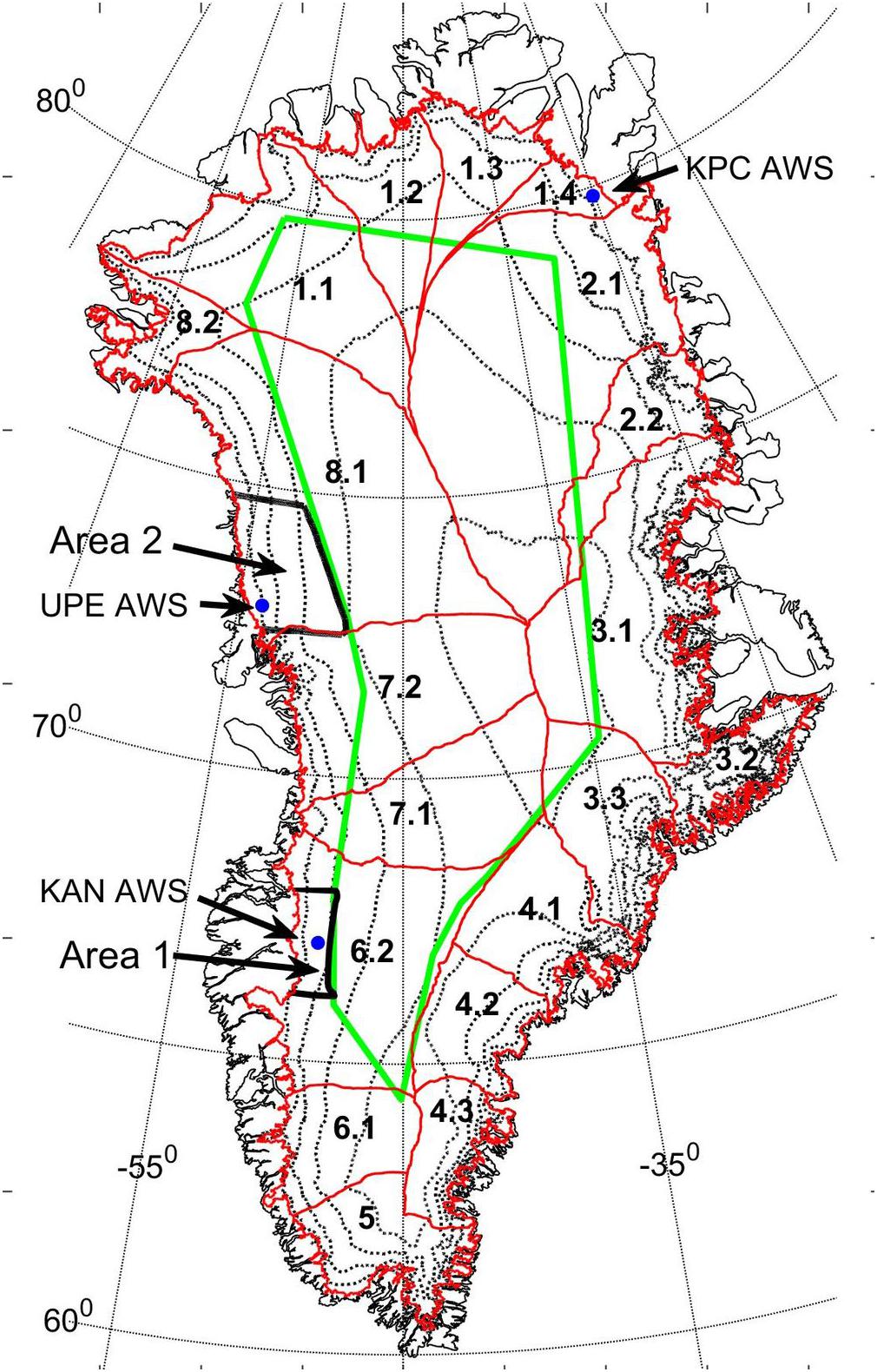
Figure 1. Illustration of the positions of the three Program for Monitoring the Greenland Ice Sheet (PROMICE) automatic weather stations (AWS) referred to in this study and the red-outlined Zwally basins. The outer red line reflects the outer edge of the ice sheet. The green line delineates the inner extent of coverage of the SARIn mode of the CryoSat radar altimeter and the outlines of the two areas referred to in the results section “Temporal Height Change in the Ablation and Lower Percolation Regions of Western Greenland” are outlined in black.

Data and Methods

CryoSat

We derived the CryoSat heights from ESA baseline C Level 1b files using the processing described in Gray et al. (2015, 2017). The estimated position of the surface is derived from each SARIn waveform by finding the point of inflection on the first significant leading edge. The algorithm which estimates the surface position from the waveform is referred to as the “retracker,” and other studies (Nilsson et al., 2016; Smith et al., 2017) have adopted a similar processing scheme.

In the cross-track direction, the slopes at the edge of the ice sheet are such that the cross-track look angle to the nearest point on the ice surface often exceeds 0.55° and 2π must then be added or subtracted to the differential phase for correct geocoding of the footprint. In our processing scheme, mapping solutions are calculated for three phase values; a slightly smoothed version of the L1b phase and that phase ± 2π (Gray et al., 2017). The Greenland Ice Mapping Project Digital Elevation Model (GIMP DEM; Howat et al., 2014) is used to help identify the most likely of the three solutions, but there is still the possibility of a mapping error, particularly if the incorrect phase solution is chosen. Large along-track slopes (>∼0.5°) affect the distribution of power in the 64 fore-aft beams or “looks” that are summed in the Delay-Doppler processing to create the waveform in the L1b file (Raney, 1998; Wingham et al., 2006). This can affect the shape of the composite waveform and thereby the selection of the position in the waveform from the retracker and the geocoding solution. The centroid of the 64 looks is available in the L1b file and is a function of the along-track slope at the footprint, the satellite pitch angle, and the vertical Doppler (which can be calculated from the satellite state vectors and the time history of the satellite height above the WGS-84 ellipsoid, Galin et al., 2014). The along-track slope can then be estimated by assuming that the line-of-sight for the strongest “look” will be perpendicular to the along-track surface.

Some editing is undertaken during the initial processing stage: The average power of the first five waveform samples should be less than −152 dB; if not it is probable that the tracking loop has missed the ice surface and no height solution value is obtained from the retracker algorithm. Some parameters are saved after the initial processing, including the along-track slope discussed above, so that further editing can be carried out in subsequent processing. In the current work, we removed retracker solutions if the along-track slope estimates were greater than 0.5°; the coherence at the position retracker point position was less than 0.7; the ratio of the waveform maximum to the average of the first 5 values was less than 6 dB; and if the leading-edge slope was less than 4.10E-16 W/sample, where the in-air sample size is 0.47 m. These values, while somewhat arbitrary, are based on minimizing the standard deviation of the difference between airborne laser and CryoSat heights which were closely spaced temporally and spatially.

We calculate the temporal height change for specific areas and elevation ranges using the point-to-point method described in Gray et al. (2015). An area is selected over which we expect the point-to-point height change to change slowly. In some regions this area can be relatively large, even 10⁴ km². Having selected the area over which we want to calculate the temporal height change the next step is to segment the data set for that area into separate time periods. The shortest practical time window is the 30-day sub-cycle of the satellite orbit (Wingham et al., 2006), but in southern Greenland the increased orbit track separation reduces the density of points and we have used 60-day time windows in some cases. To estimate the average temporal height change, every height point in one time period is compared with every point in all the other time periods. While this is computationally tedious, it does have an advantage in that it provides a method for removing poor values. If the distance between the two points is less than a preset limit, usually 400 m, the height difference is saved. In this way the mean and standard deviation for that area and time difference are available and a criterion can be used to eliminate values that exceed the criterion. In the current work height differences of greater than 10 m from the mean were removed. As the standard deviation of the individual height change estimates is typically 1.5 to 3 m, this exceeds the often-adopted criterion of ± 3 standard deviations.

The success of this approach depends on the total number of height estimates and the size of the area used. Ideally each 30- or 60-day time period should have ∼1000 or more height samples, and in the comparison of any two time periods there should be at least 100 pairs of points satisfying the separation criterion. When comparing the average height change from one time period (A) to two other time periods (B and C), different points will be used in creating the AB height change and the AC height change. Consequently, an independent estimate of height difference AB can be obtained by calculating AC – BC. This allows a check on the consistency and statistical error in the results. For example, if there are 100 30-day time periods in the overall results then there are 99 estimates of the height difference from the first time period to any subsequent time period; one direct estimate between the two time periods and 98 estimates involving an intermediate or subsequent period (Gray et al., 2015). In creating the final average height difference a weight of 1 is used for the direct estimate and a weight of $1/\sqrt{2}$ for those estimates which use an additional time period. For any height change result an approximate statistical error is given by the average of the standard deviations divided by the square root of the number of samples. In the temporal height change plots, the vertical bar at each height change is ± 2 times this estimate, typically ± 10 cm. However, this is an underestimate of the potential error in surface height change as it neglects the effect of a possible variation in bias between the surface and CryoSat height with changing conditions, and the fact that the height samples may not be uniformly distributed in either time or space. CryoSat data are only available for some days during each 30- or 60-day time period, the average height of the samples in any time period may be slightly different from those in another, and the spatial distribution of the samples in the overall area will be slightly different for each time period. These complications can lead to additional bias errors which are hard to quantify, however, attempts to monitor, measure and minimize them are on-going.

Two main processes have led to ice sheet ice loss over the last 10–20 years: meltwater run-off has increased (Van den Broeke et al., 2009), and ice flux has increased through a change in ice dynamics (Rignot and Kanagaratnam, 2006; Joughin et al., 2018). Because the change in ice dynamics can affect areas smaller than those we have used for the 30- or 60-day height change results, we have modified our method to provide better spatial resolution for the height change results in this case. In this modification of the data processing, we increase the duration of the time window to try to offset the reduction in the area sampled. Images of height change have been included in the results for the north-west and north example areas. The spatial sampling for these examples was 0.1° in latitude (11.1 km) and 0.2° in longitude (5.8 km at 75°N) with a bin size of 0.2° in latitude and 0.4° in longitude (∼65 km²), and a temporal bin size covering the winter from mid-October to mid-May.

Airborne Ku-Band Altimeter

Data from the airborne Ku-band altimeter measurements over Greenland (Patel et al., 2015; Leuschen et al., 2017) were downloaded from the NSIDC Operation IceBridge web site portal¹. Individual files span ∼33 s, cover ∼5 km along-track, and include the position and elevation of the aircraft and all the necessary timing and radar parameters required for subsequent data analysis. The range resolution of the airborne Ku altimeter is much better than that of the CryoSat SARIn data. The bandwidth, and therefore range resolution, of the airborne altimeter was 3.5 GHz in the 2011 spring Greenland campaign, and 6 GHz in subsequent years. This is more than an order of magnitude better than the 0.32 GHz bandwidth used in the CryoSat SARIn mode.

Each waveform is converted to the amplitude domain from the logarithmic dB format and smoothed with a filter designed to reduce high frequency noise. The aircraft height above the surface is calculated using the delay time for which the return amplitude first reaches a particular amplitude. The minimum of all the maximum amplitudes of all the waveforms in the file is obtained, and the surface is estimated to correspond to the point in each waveform at 35% of this value. Samples from 100 points before the detected surface to 899 points after the detected surface are merged for the desired sequence of files. After smoothing, the airborne Ku altimeter vertical resolution in the near-surface snow layer (assuming a density of ∼340 kg/m³ and permittivity of ∼1.6) is reduced from ∼3 to ∼10 cm. Although the snow/firn density and permittivity will change with conditions and depth (Fausto et al., 2018), this will only affect the depth scale on the figures illustrating the airborne Ku-band results and doesn’t affect the conclusions or comparison with the CryoSat results. For presentation purposes, averaging is also carried out in the along-track direction: eleven waveforms are averaged, and the averages are saved at a spacing of five waveforms. Smoothing along-track is then over ∼50–60 m and the result is sampled at 25–30 m. For visualization purposes, the results are converted back to the dB format.

Airborne Lidar Surface Height Measurements

The NSIDC web portal² provides a convenient link to access many years of NASA airborne laser scanner data. We have used the Level 2 (L2) ATM data (Krabill et al., 2002; Studinger, 2018) as a surface height reference in order to check the accuracy with which CryoSat can estimate surface height change. The accuracy of these data for surface height measurement is better than 12 cm with a precision of 9 cm (Brunt et al., 2017). All the heights, including those from the CryoSat processing, are referenced to the WGS 84 ellipsoid. In comparing results from the airborne laser scanner with Cryosat heights and height change, it is important to acknowledge that the footprints and temporal acquisitions are quite different. Individual ATM L2 footprints are at least two orders of magnitude smaller in area than the CryoSat footprints. Often the IceBridge flight lines were repeated each spring so that height change over an area could be estimated by averaging the height difference of pairs of footprints whose centers were less than 10 m apart. This method was used in estimating average surface height change between the spring and fall of 2015 and 2016 over the area 1 in Figure 1. This approach is possible provided that the area over which the averaging is done does not include large changes in height loss, e.g., the Jakobshavn Glacier, and that both averages are representative of the whole area.

Year-to-year surface height change data are also available on the NSIDC web site (Level 4, ATM³, Studinger, 2017). We also used these data in comparing CryoSat and airborne laser height change for yearly spring-to-spring periods for specific areas. Again, we derived the average height change independently for CryoSat and the ATM L4 height change results over specific areas. Again, with this approach it is necessary to check that the average heights were comparable and that the distribution of CryoSat and ATM L4 points in the sampled areas was comparable and reflected the area in question. For these comparisons the time window for CryoSat acquisitions about the airborne acquisition was typically ∼2 months.

PROMICE Automatic Weather Station (AWS) Data

Program for Monitoring the Greenland Ice Sheet (PROMICE) is operated by the Geological Survey of Denmark and Greenland (GEUS), in collaboration with the Technical University of Denmark (DTU Space), and Asiaq, Greenland Survey. The program maintains AWSs in eight areas around the Greenland Ice Sheet with 2 – 4 AWS’s at different elevations in each of these areas, but mostly in the ablation zone (Van As et al., 2011).

Standard meteorological parameters are recorded every 10 min (temperature, pressure, wind speed, direction, etc.), as well as hourly position from a single frequency GPS receiver. More specialized sensors adapted for ice sheet monitoring include; a radiometer for measuring down- and upward radiative fluxes, sonic rangers to monitor relative surface height change associated with local accumulation and melt; and a buried pressure transducer to provide data on mass loss above the transducer (Fausto et al., 2012; Fausto and van As, 2019).

Results

Temporal Height Change in the Ablation and Lower Percolation Regions of Western Greenland

Figure 2A illustrates an area north and south of the PROMICE KAN-M AWS that has had coverage from IceBridge flights every spring, and in the fall of 2015 and 2016. Although the footprint sizes and sampling in time are quite different, Figure 2B illustrates the good agreement between the CryoSat and laser scanner height changes averaged over the same region, including the height change associated with summer melt and winter accumulation for both 2015 and 2016. When an ice sheet is in long-term equilibrium the upward, emergent ice movement below the equilibrium line altitude (ELA) in the ablation zone would balance the net ice ablation and provide similar ice heights in the long-term (Cuffey and Patterson, 2010). However, we see that there has been a net thinning of 3–4 m since the winter of 2011 and that the area below 1300 m elevation (fawn data in Figure 2B) lost more height than the area above 1300 m (light blue data).

FIGURE 2

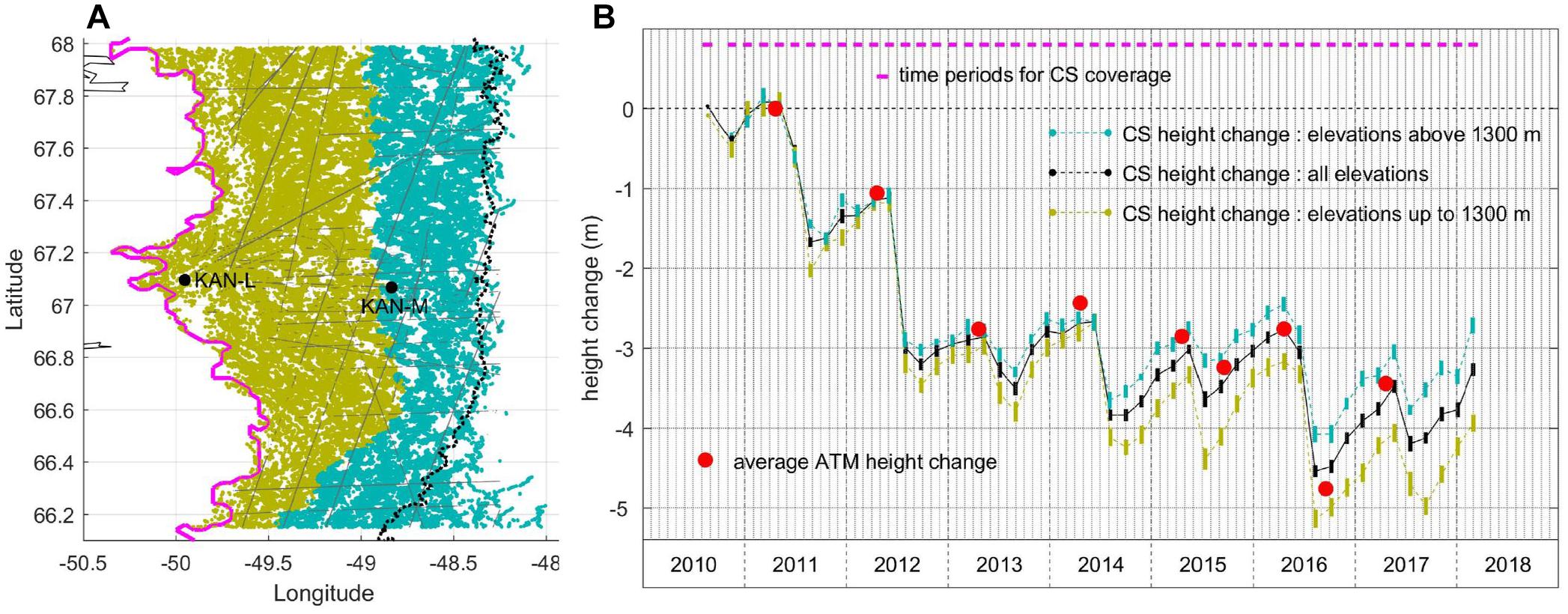
Figure 2. (A) Positions of the CryoSat height estimates for two elevation ranges, above (87,000 samples in light blue) and below 1300 m (79,500 samples in fawn), and of two of the PROMICE KAN weather stations. The solid magenta line indicates the ice sheet edge and the dotted black line is the 1500 m contour. IceBridge laser terrain mapper (ATM) data were collected in this area in the springs of 2011 to 2017 and in the falls of 2015 and 2016, and their positions are shown by the gray dots. (B) Temporal height change with respect to the winter 2011 for all the data (black), data < 1300 m (fawn) and data > 1300 m (light blue). The data was binned in intervals of 60-days, the actual time periods are shown as the sequence of short magenta lines at the top of B. The red dots illustrate the ATM height change averaged over the same geographic area and referenced to the spring of 2011.

The KAN-M AWS at 1270 m elevation also provides evidence that the Cryosat height changes can follow at least relative melt. The buried pressure transducer at KAN-M showed net summer ablations of 2.1 ± 0.2 m (2012), 0.8 ± 0.2 m (2103), 2.2 ± 0.2 m (2016) and 0.5 ± 0.2 m (2017), compared to the average CryoSat height losses of 1.9 ± 0.3 m (2012), 0.6 ± 0.3 m (2013), 1.8 ± 0.3 m (2016), and 0.7 ± 0.3 m (2017) for the whole area in Figure 2A. The long-term mean ELA (1990–2011) in this area was estimated to be 1553 m (Van de Wal et al., 2012), and subsequent work (Smeets et al., 2018) suggests a continuing upward trend in the long-term ELA. At this latitude (67°N) in western Greenland the SARIn mode data is restricted to elevations less than ∼1500 m so that all the available SARIn data in this area is normally from the ablation zone. Any quantitative use of CryoSat surface height change in terms of snow accumulation or summer melt needs to consider the vertical component of ice movement. In the ablation zone there will be a vertically upward, emergent component to the particle path motion (Cuffey and Patterson, 2010), and this component will increase as the elevation decreases down-slope from the long-term ELA region between the accumulation and ablation zones. While the weather stations do record GPS data these are not accurate enough for precise vertical displacements. Consequently, in this area we would expect the temporal CryoSat height change results to be less than that associated with net ablation and sublimation. For this time period, the plots in Figure 2B show the large melts in increasing order, for 2011, 2016, and 2012, the relatively low melt seasons in 2013 and 2017, and the relatively high accumulations for the winters of 2013/14, 2015/16, and 2016/17.

In summary, the airborne Ku-band radar altimeter normally exhibits a strong surface return in west Greenland, and we show that the CryoSat height change history averaged over an extended area around the KAN–M weather station is in good agreement with the surface height change derived from the airborne laser scanner averaged over the same area.

Temporal Height Change in a High Loss Area in North-Western Greenland

The north-western coastal area of Greenland has exhibited significant ice loss in recent decades (Kjeldsen et al., 2013). The net ice flux from most of the outlet glaciers in this area continues to increase (Joughin et al., 2018) and this, coupled with recent increase in meltwater run-off (Van den Broeke et al., 2016), has made this a key area for measuring temporal change in ice loss. Here we link the CryoSat height changes to changes in ice speed, and to information from the PROMICE UPE-U AWS that is situated between two arms of the Upernavik glacier and is moving at ∼200 m/year.

Over the lifetime of CryoSat we have ∼780,000 height estimates from the ∼40,000 km² area shown in Figure 3A. The large ice loss in this area is concentrated at the lower ice sheet elevations and is illustrated by the average 30-day height change for the Cryosat points between the edge of the ice sheet and 1400 m elevation (Figure 3B). The Cryosat height loss, and by inference average ice loss, is then less for the elevation range from 1400 to 2000 m, and even less in the range 2000–2600 m. Figure 4A illustrates the speed change between 2009 and 2016 (Joughin et al., 2018), and the spatial distribution of the 7-year Cryosat height change (Figure 4B) as a color overlay on a Radarsat image mosaic (Joughin et al., 2016). The height change has been calculated using a spatial window of 0.2° in latitude (22.3 km N/S) and 0.6° in longitude (19.6 km E/W) sampled at 0.1° in latitude and 0.3° in longitude with a 7-month winter-spring time window. (15 October to 15 May).

FIGURE 3

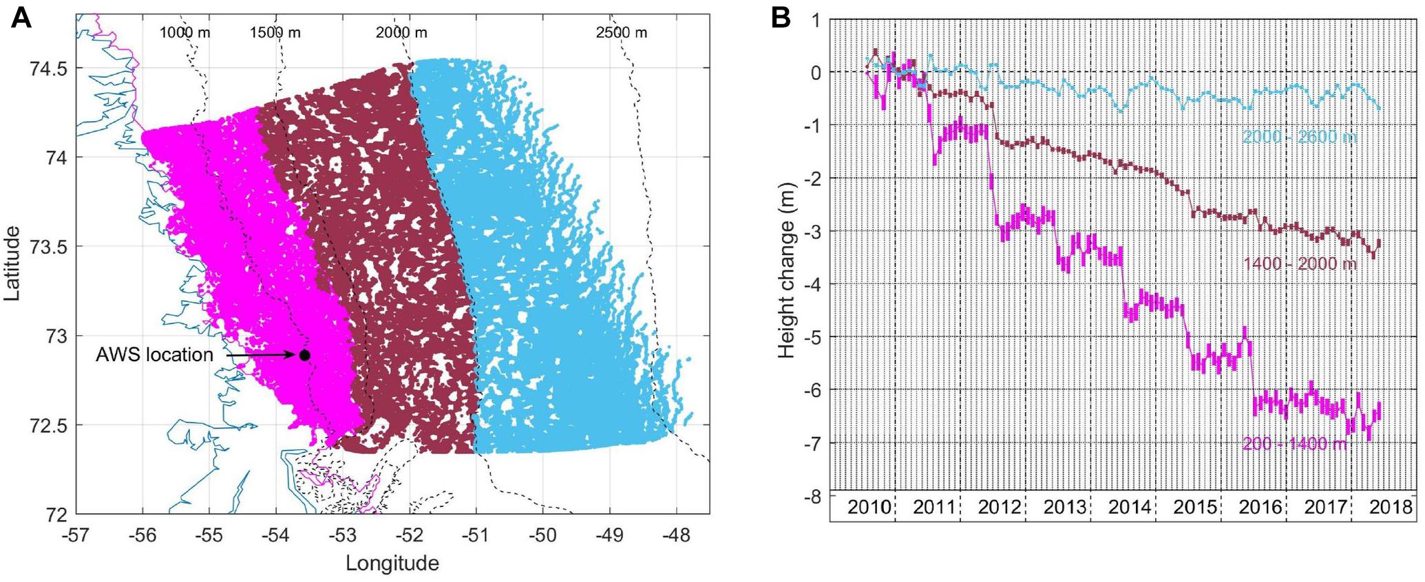
Figure 3. (A) The positions of the CryoSat data from three elevation ranges in NW Greenland (Area 2 in Figure 1) are illustrated in color (272,105 samples > 2000 m in blue; 342,119 samples 1400–2000 m in maroon; 169,029 samples 200–1400 m in magenta). The position of the UPE-U AWS is shown by the large black dot. (B) The average temporal height change for the data in the three elevation ranges is shown in B. In this case the temporal CryoSat height change has used 30-day bins.

FIGURE 4

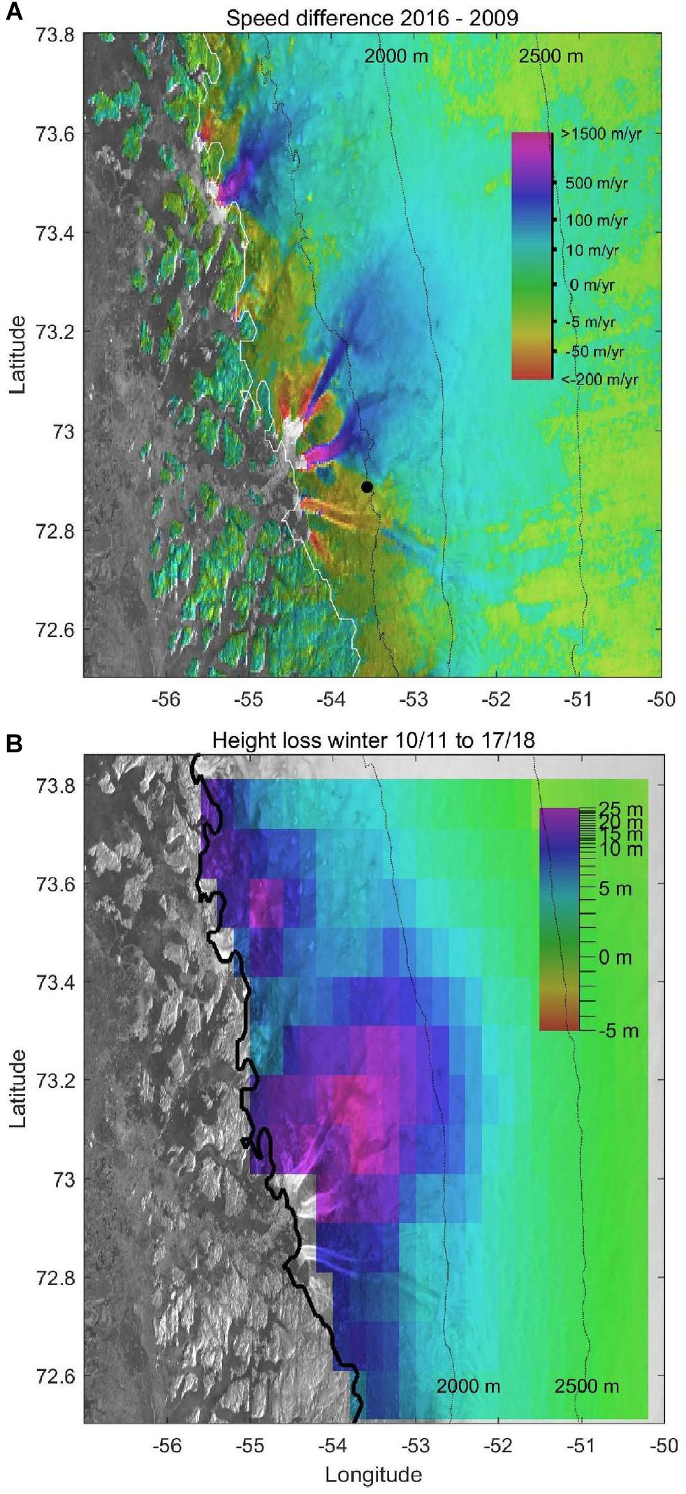
Figure 4. (A) The difference in ice speed between the winter of 2016/17 and 2009/10 is shown as a color overlay superimposed on a Radarsat mosaic image of the ice sheet. The position of the UPE-U AWS is shown by the black dot. (B) Height change between the winter/spring of 2010/11 and the same period in 2017/18 again illustrated as color on the Radarsat image.

The height loss over the CryoSat time frame is particularly large close to two of the northern arms of the Upernavik glacier (Andresen et al., 2014), and this is related to the increased ice flux across the grounding line over almost the same time period. There are three large branches of the Upernavik glacier, two north of the UPE AWS (black dot in Figure 4A) and one south. The change in speed for these branches was documented by Larsen et al. (2016) up to and including 2013. This study showed that of the two large branches north of the weather station position, the northern branch sped up first. The recent speed change data (Figure 4A) shows that the southern branch of the pair has now sped up significantly while the other has slowed at the edges of the glacier close to the coast, but the upstream speeds for both are still larger in 2016/17 than in 2009/10. In this area the increase in ice speed from 2009/10 to 2016/17 has led to the large height loss shown by the Cryosat results. Note that the third arm of the Upernavik glacier south of UPE-U has slowed slightly in the same period and the height change is much more modest in this area. This shows that the balance between ice loss due to melt run-off and that due to increased outlet glacier speed can be quite different, even over relatively small distances.

The ablation pressure sensor at UPE-U shows the large melt each summer (Figure 5A, blue). The year-to-year absolute height change from CryoSat has been interpolated to the weather station site (Figure 5A, magenta) and mirrors the local surface ablation but the overall magnitude is about 20% less. The comparison of the year-to-year height change between the CryoSat results and the pressure sensor (Figure 5B) shows a good correlation except for the 2011 – 2012 and 2012 – 2013 differences where the pressure sensor height losses are more than that estimated from the CryoSat data. The CryoSat data is an average over the winter; from October 15 to May 15 and covers a relatively large area (∼65 km²⁾, whereas the pressure sensor data has been selected at 15 Feb. each year and represents the ice loss at one location. As at KAN-M, the local surface height change from the ablation sensor does not include the upward emergent component of ice movement. As the UPE-U AWS is in the ablation zone, this may explain at least part of the difference between the two plots.

FIGURE 5

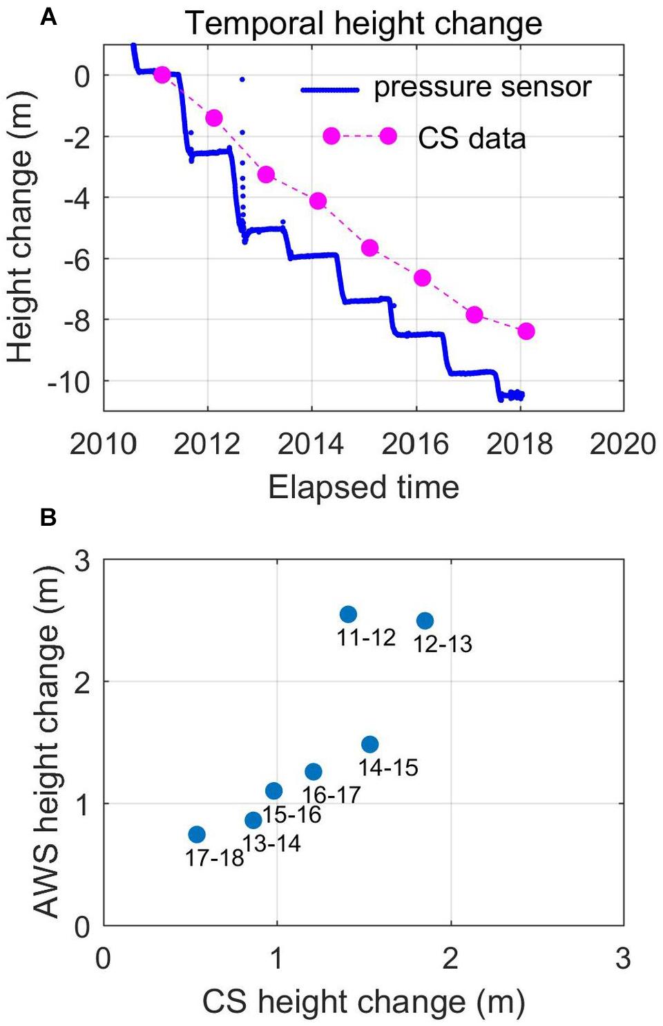
Figure 5. (A) Ice melt from the UPE-U AWS ablation pressure sensor is shown in blue, and the winter-to-winter CryoSat height change interpolated to the position of the UPE-U AWS is shown in red. (B) Plot of the winter-to-winter height change for the CryoSat and ablation sensor data (at 15 February each year).

Impact of High Accumulation and Spring Melt on Derived Heights

We illustrate the influence of winter snow accumulation on CryoSat results by comparing the temporal height change derived for two basins (Figure 6A) in southern Greenland. The annual accumulation is much larger (1–3 m) in basin 4.3 on the east side of the central divide than in basin 6.1 (<1 m) on the west (Hanna et al., 2006; Koenig et al., 2016). The 30-day temporal CryoSat height change for three different elevation ranges for basin 6.1 is shown in Figure 6B and for two elevation ranges in Figure 6C for basin 4.3. The temporal height change plot for the lower elevation range (500–2000 m) for the western basin 6.1 reflects summer melt and winter accumulation, and illustrates the large melts in 2012, 2011, and 2016, and the much weaker melt seasons in 2013, 2015, and 2017. The temporal height changes for the two elevation ranges for the eastern, high accumulation, basin 4.3 are quite different. In particular, there is a significant decrease in CryoSat height over the winter months. In the winters of 2014/15 and 2016/17 the Cryosat height decreases by ∼2 m in the 2500–2930 m elevation ranges and slightly more in the 100–2500 m elevation range. We explain this apparent anomaly using airborne Ku-band radar and laser results.

FIGURE 6

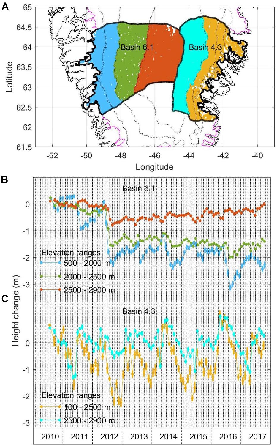
Figure 6. (A) Positions of the CryoSat footprints for three elevation ranges in basin 6.1 (167,792 blue samples, 207,437 green samples, and 211,661 brown samples) and two (125,92 light blue samples and 225,728 fawn samples) in basin 4.3. The 30-day temporal height change in meters with respect to the winter of 2010/11 is shown for the different elevation ranges in basin 6.1 (B) and basin 4.3 (C).

Under cold spring conditions the dominant reflecting layer for airborne Ku-band radar altimeters is often the last-summer melt layer (Hawley et al., 2006; Helm et al., 2007; Patel et al., 2015). The airborne Ku-band waveform (Figure 7) from the April 13, 2015 flight-line segment CD in Figure 8 at ∼64°N has been averaged over 1.1 km and shows an initial peak corresponding to the snow surface and a much stronger delayed peak corresponding to the sub-surface high-density layer from the last-summer melt. Four days after the NASA flight on April 17, 2015 the same area was covered by CryoSat. However, the surface and delayed returns from the melt layer were not resolved in the average of over 70 CryoSat waveforms (red line in Figure 7) because of the much larger footprint size and coarser range (height) resolution. The 380 m along-track footprint size (Bouzinac, 2012) is defined by the Delay-Doppler processing (Raney, 1998), and in the cross-track direction by the range resolution and the cross-track surface curvature. We used the GIMP DEM (Howat et al., 2014) to estimate the cross-track footprint size for this area. The resulting distribution was broad and asymmetric with a median value of 438 m. Consequently, assuming there are no strong specular reflections from, e.g., a wet ice surface or supraglacial lake (Gray et al., 2017), the average CryoSat footprint is a few thousand times larger than the footprint area of the airborne Ku-band altimeter. While the incident wave is perpendicular to the surface at the area of closest approach, the returns from the last summer layer are range ambiguous with surface returns from both sides of the cross-track retracked position. The “shoulder” on the leading edge of the red waveform in Figure 7 is suggestive of a surface return, but the algorithm used in this work to identify the CryoSat surface height from the waveform corresponds more closely to the strong subsurface returns in this region.

FIGURE 7

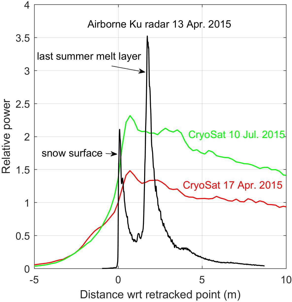
Figure 7. Comparison of CryoSat (red and green), and airborne Ku-band altimeter waveforms (black) from close to the intersection of IceBridge flight lines CD and EF in Figure 8. The red and green waveform plots are averages of all the CryoSat waveforms from two closely spaced descending passes (EF) on April 17, 2015 and July 10, 2015, between 63.9° and 64.1°N. The x axis is range distance from the position estimated from the retracker algorithm.

FIGURE 8

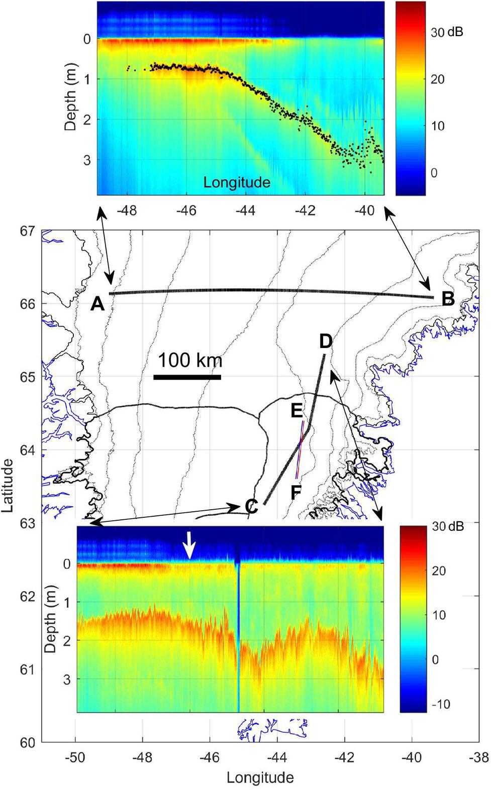
Figure 8. The positions of two airborne IceBridge Ku-band altimeter flight line segments from April 13, 2015 are marked as AB and CD. The two insert images illustrate the airborne Ku-band altimeter results in which the waveforms have been aligned, smoothed along-track, and the return power in dB represented in color. The white arrow in the lower insert image indicates the position of the airborne Ku-band waveform in Figure 7. The black dots in the upper insert image show the estimated depth of the last-summer melt layer in meters and the strong west-east gradient in snow accumulation. The two closely spaced lines at EF are the positions of two CryoSat passes from April 17, 2015 and July 10, 2015. Part of the boundaries of basins 6.1 and 4.3 are shown on either side of the central ice divide. The limit of the ice sheet is marked in black and the coastline in blue.

The shape of the CryoSat waveforms is dictated by the size and condition of the surface and near-surface patch contributing to the sequence of range gate cells in the receive window. By July 10, the average waveform for this location (green plot in Figure 7) has a larger peak amplitude, a steeper leading edge and, as implied by Figure 6C, the derived height increases in relation to the April results. This is consistent with increased near-surface snow moisture, leading initially to reduced returns but as melt progresses to a stronger surface reflectivity and decreased or eliminated returns from the last-summer melt layer (Wang et al., 2016; Gray et al., 2017). Consequently, we suggest there are two mechanisms leading to the apparent decrease in derived height between the late-fall and winter in the high accumulation basin 4.3: the strongly reflecting last-summer melt layer will sink with accumulation and firn compaction during the winter, and over the same time the thickening dry snow layer above the melt layer acts as a dielectric, slowing the radar waves and contributing to the apparent decease in CryoSat height.

NASA flew some of the Greenland lines in the fall of 2015 as well as in the spring of both 2015 and 2016, thus providing a convenient way of measuring the downward movement of the last-summer layer due to firn compaction associated with overlaying snow and firn. We use data collected over part of the CD flight line segment in Figure 8 to illustrate the method. Using the surface height difference between fall 2015 and spring 2016 from the airborne laser terrain mapper data, and the depth of the last-summer layer from airborne Ku-band altimeter data from the spring 2016 flight, we estimate the absolute vertical downward movement of the 2015 melt layer between the fall of 2015 and the spring of 2016 (Figure 9A). If there was some accumulation on top of the denser summer layer by the time of the fall flight on October 13, 2015 then the 1.5–1.8 m estimate of vertical downward movement of the last-summer melt layer at ∼2500 m elevation may too large. If the last-summer layer provides the dominant contribution to the CryoSat waveform then the reduction in the height estimate due to the change in wave speed in the winter snow layer is $\left(n-1\right)D$, where $n$ is the refractive index of the near surface snow layer and $D$ is the thickness. Using $n=1.27$ this would lead to an additional apparent height decrease of ∼0.27 m per meter of snow above the last-summer melt layer. This very likely overestimates the bias in the estimated surface height because the reflection from the snow-air interface will also contribute to the measured waveform so that the height estimate will fall somewhat between the surface and the (biased) last-summer height. This effect, a decrease in derived height over the winter months, was also observed in basins 4.2 and 4.1. Data from an elevation range from 2000 to 2600 m, was used and the results showed that the magnitude of the winter height reduction was less in these basins, especially for basin 4.1.

FIGURE 9

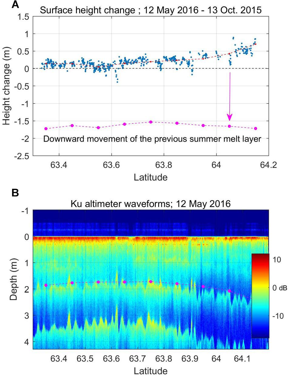
Figure 9. (A) The small surface height increase from October 13, 2015 to May 12, 2016 has been derived from the repeat airborne laser scanner data along part of flight line CD in Figure 8 and is shown as blue dots. The approximate position of the last-summer melt layer with respect to the October 13, 2015 surface is plotted as a dashed magenta line. (B) The pseudo image of the May 2016 Ku-band airborne Ku-band altimeter data shows the last summer melt layers from both 2014 and 2015. The dashed magenta line indicates the approximate depth of the 2015 last-summer layer which was used in estimating the approximate downward movement of the 2015 melt layer.

It is important to emphasize that under cold spring conditions, the relative contribution from the last-summer melt layer may vary from year-to-year as the strength and duration of melt can vary year-to-year. Note that the contribution from the 2015 last-summer layer in the May 12, 2016 airborne Ku waveforms (Figure 9B) is less than the surface contribution, and apparently less than the 2014 last-summer layer in the 2015 spring Ku waveforms. This difference probably reflects the fact that the spring 2016 flight was on 12 May and the snow surface had changed to the point that the dominant returns were now from the surface. Also, in Figure 9B showing the stacked Ku altimeter waveforms from May 2016, we can see the returns from the buried dense layers from the summers of both 2015 and 2014, but in the April 13, 2015 plot from the same area (Figure 8) it appears that the dense layer from summer 2013 is absent. The conclusion from these observations is that winter-spring CryoSat height estimates in this region can depend quite strongly on the meteorological conditions and history in a way that makes interpretation difficult. Two approaches could be used to minimize this problem: changing the retracker algorithm that picks the height to one that positions the “surface” on the early part of the waveform leading edge (Davis, 1997; Helm et al., 2014), or simply ignoring the winter-spring data and estimating year-to-year height change by concentrating on the late summer-early fall data when the returns are predominantly from the surface. Neither approach is ideal, but we favor the latter as it is difficult to eliminate the effect of the strong sub-surface returns.

Height Change in a Northern Basin; Winter Accumulation and Summer Melt

Figure 10A shows the positions of the PROMICE KPC-U weather station (870 m elevation) and the CryoSat data for three elevation ranges in basin 1.4 in northern Greenland. The 30-day average temporal height change plots over the three elevation ranges are shown in Figure 10B. As expected, the height loss is primarily at the lowest elevation range, up to 1100 m, and shows a clear annual variation related to winter accumulation and summer melt. Figure 10C shows the spatial distribution of height loss between the winters of 2010/11 and 2016/17. In this basin there are no large marine-terminating outlet glaciers with changing ice flux, and the height loss has occurred primarily along the ice sheet edge with slightly more in the SE corner, adjacent to the large 79N-fjord glacier.

FIGURE 10

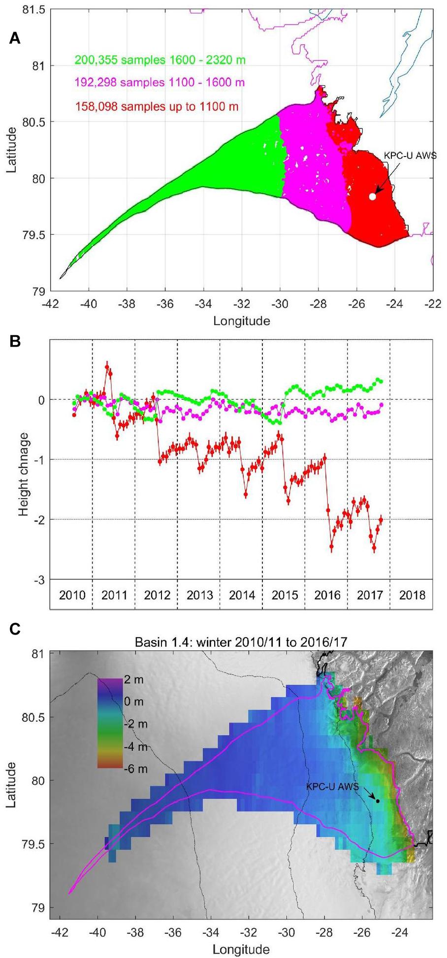
Figure 10. (A) The red, magenta and green colored dots indicate the positions of the Cryosat data in basin 1.4. The elevation ranges are: red; ice sheet edge to 1100 m, magenta; 1100–1600 m, and green; 1600–2320 m. (B) Temporal height change for the three elevation ranges in A. (C) Six-year height loss derived from Cryosat data. Position of the KPCU AWS is shown with the black dot.

We compare the KPC-U AWS ablation/accumulation data with the CryoSat height change for the area up to 1100 m. The mean height for this area is the same as the weather station height (∼870 m) and is approximately equal to the average ELA over this time period. Figure 11 illustrates the comparison between the average CryoSat height change over the blue area in Figure 10A with the local relative surface height change measured by the sonic ranger attached to a stake assembly frozen in the ice. To improve the comparison, we have assumed a constant downward movement of the stake assembly of 0.29 m/year. With this assumption, the correspondence between the average height change for the blue area in Figure 10A and the local height change at the weather station is clear. For example, the CryoSat data has captured snow events in the late spring of 2011, and the low accumulation in the winter of 2012/13. Although there are differences, the two plots have similar shapes and the CryoSat data mirror the local height change related to accumulation and melt. However, the temporal height change for the green curve (CryoSat samples from 1600 to 2320 m) in Figure 10B often exhibits a decreasing height in the winter months and an increase in height in the summer. For example, from fall 2011 to late spring 2012 the CryoSat height decreases by 40 ± 10 cm but then increases by about the same amount in mid-summer 2012. Considering the ice sheet wide warming in July 2012, it is very unlikely that the average surface height at these elevations (1600–2320 m) increased at exactly the time when the lower elevation range loses ∼1 m in elevation. It is much more likely that there is a seasonal variation in the bias between the actual and the detected surface, and that the surface elevation between 1600 and 2320 m either changed little or decreased during the warm summer of 2012.

FIGURE 11

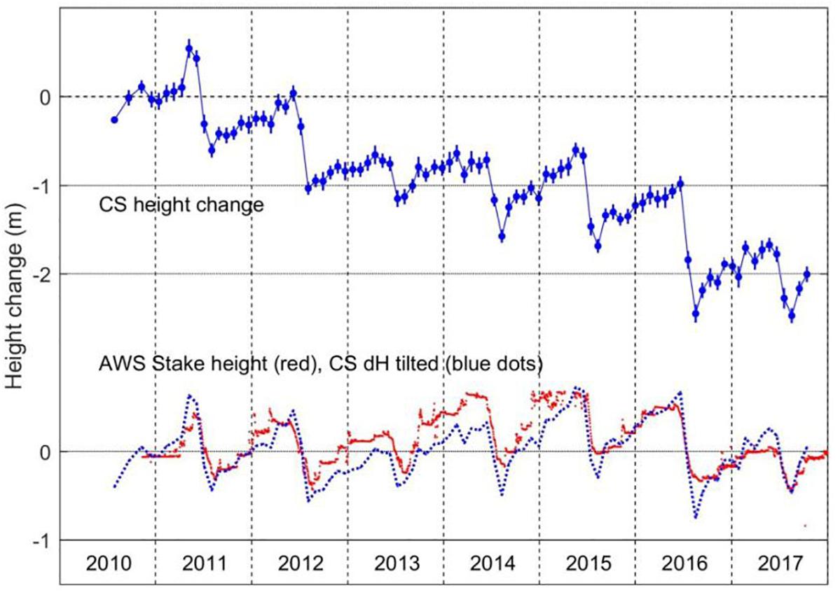
Figure 11. Illustration of the correlation between the temporal height change from the CryoSat data (upper blue plot) and the relative height change from the stake mounted sonic ranger sensor on the KPCU AWS (lower red plot). The blue dotted plot superimposed on the red AWS stake height plot is the height change corrected for an assumed constant downward motion of the AWS.

Further tests were carried out in basin 1.3 to the west of basin 1.4 to check whether this anomalous height change result existed elsewhere along the northern ice sheet. The test site is 20 km EW and 275 km NS and extends into the accumulation zone at the higher elevations (Figure 12). The temporal height change is shown for two elevation ranges above and below 2000 m in the upper insert plot, and the results mirror the high elevation band from basin 1.4 shown in Figure 10B. In addition, waveform data are selected from three descending passes from September 2011, from three descending passes in the same area from April 2012 prior to the onset of the summer 2012 melt, and from three descending passes from September 2012. The 2012 fall lines overlap the 2011 fall lines due to the satellite’s 369 day repeat cycle. By averaging over 2,000 waveforms for each period, we see that there is a systematic change in the waveform shape and peak amplitude. The width of the average 2012 April waveform at half height is 155% wider than the average waveform from fall 2011 and over twice as wide as that from fall 2012. We expect that the shape of the first peak in the waveform reflects composite surface and volume scattering modulated by the size of the cross-track footprint created by the surface slope and slope curvature. It is reasonable to assume that due to the increased summer temperatures and solar insolation, the surface will become more reflective due to densification of the near-surface layers. As a result, we expect that the first return width will decrease, and the leading edge will steepen as the surface component to the composite return increases. This is exactly what is observed here and in other higher elevation test sites across the northern edge of the ice sheet. This again implies that changing conditions from the previous summer can change the subsequent winter and spring waveform shape in a way that could lead to a changing bias between the surface and the CryoSat detected surface height. We note a significant increase (∼45 ± 10 cm) in the average CryoSat height occurred in the summer of 2015 in basin 1.4 (green data in Figure 10B) and in other test sites above 2000 m across northern areas of the ice sheet, and that summer temperatures were above normal in this region in 2015 (Tedesco et al., 2016).

FIGURE 12

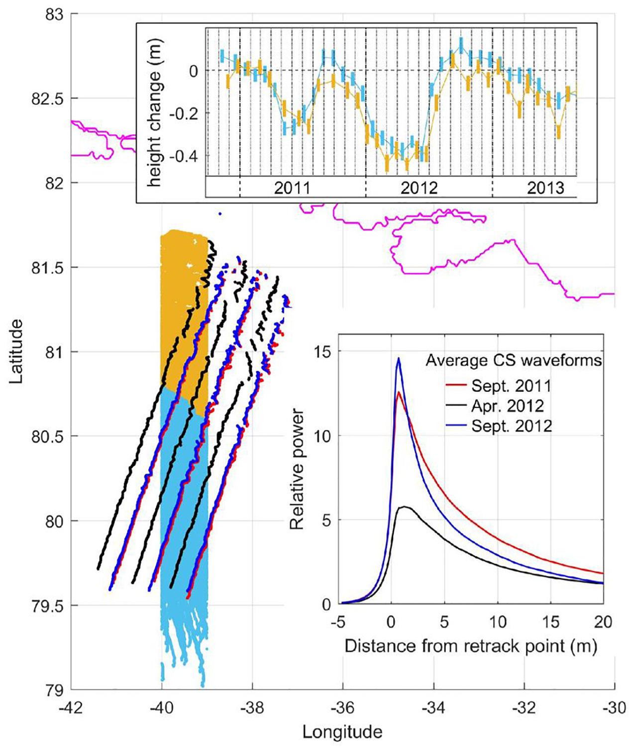
Figure 12. Positions of the CryoSat data in the basin 1.3 test site are shown as 88,906 fawn dots (<2000 m) and 100,182 light blue dots (>2000 m). The 30-day temporal height change derived from these two data sets are shown in the upper insert plot using the same colors. Over 2000 CryoSat footprint positions are shown from each of 3 descending passes in 3-time frames; September 2011 in red, April 2012 in black and September 2012 in blue. The average waveform from each time frame is plotted in the lower insert graph using resampled waveforms such that the retracked position was set to zero.

Discussion and Conclusion

Since its commissioning in 2010, the ESA CryoSat SARIn mode has demonstrated excellent temporal and spatial coverage and an improved ability to track surface height change in comparison with radar altimeters that do not use dual-channel interferometric Delay-Doppler processing. In comparing the ability of CryoSat SARIn mode to track peripheral ice loss with other techniques, the following points should be made: while satellite laser altimeters, like ICESat, can provide more accurate estimates of surface heights in comparison with CryoSat, the relative paucity of results has led to the need to fit the temporal height change to a model, for example the seasonal variation is often modeled as a sinusoid. As shown here, model fits are not required with CryoSat data and, except for the SE ice sheet, 30-day or 60-day temporal height change results can track winter accumulation and summer melt. Data from the Gravity Recovery and Climate Experiment (GRACE) satellites have provided mass change estimates but the spatial resolution is low, and it can be difficult to isolate the ice sheet mass change from the overall mass change.

We relate the varying bias between the true surface elevation and the CryoSat detected elevation in the SE ice sheet to the changing dry snow layer accumulating in winter above the denser, more radar reflective, previous summer melt layer. IceBridge data have allowed an estimate of the downward motion of the last summer melt layer that supports our explanation of the varying bias. The waveform leading edge shape reflects the composite surface and subsurface returns. Changing conditions may then change the leading edge such that the detected or “retracked surface” also changes with respect to the true surface. While the magnitude of the problem may be less with a threshold retracker which uses an early time on the leading edge (Davis, 1997), it will exist to some extent for basin 4.3 data with any of the possible algorithms. In this regard, prior experiments over ice sheets and ice caps (Helm et al., 2014; Nilsson et al., 2016; Gray et al., 2017; Sørensen et al., 2018) have shown that algorithms which use the first significant leading edge in the SARIn waveforms provide more accurate estimates of surface height change than algorithms that use the whole waveform. While smaller than the effect in the SE, results from the accumulation zone in the northern periphery of the ice sheet also show a similar seasonal change in the bias between the detected surface and the real surface. As a result, we recommend that year-to-year surface height change with SARIn data, particularly in the SE, are best done with data collected in the late summer and fall period to minimize the possibility of a varying bias between surface height change and that estimated with the altimeter data.

To make an estimate of the winter accumulation or summer melt with the temporal height change plots, one must pick an area over which the average net vertical motion is very small. To do this we have selected areas with an average elevation equal to our estimate of the long-term ELA; the last-summer-layer moves slowly downward above this elevation and upward below it. In comparing these CryoSat data with some of the PROMICE AWS data, it is important to remember that very different measurements are being made. The weather station data are site specific and the estimates of accumulation and melt are made from a moving platform so that absolute vertical displacements are not normally measured. While the weather station data represent an area around the station, the relative scarcity of surface measurements around Greenland does limit the ability to validate surface mass balance models that are currently an important element in tracking ice loss. The CryoSat estimates of accumulation and melt on the other hand are based on grouping data over a large area and time period, usually 30 days, so that a lot of averaging is involved. Although the accuracy for these measurements is still being evaluated, these initial results suggest that this capability can complement other approaches for assessing yearly ice loss and snow accumulation.

In the nine-year CryoSat lifetime to date, there has been significant and widespread change in the speed of many of the outlet glaciers around Greenland (Joughin et al., 2018). Here we link the change in speed with change in upstream height by showing the significant ice loss in the area where the northern two arms of the Upernavik Glacier have sped up. Again, this illustrates the possibility of complementarity between two techniques involved in estimating mass balance. Further, by using larger time windows it is also possible to preserve enough spatial resolution to see the surface draw-down associated with changes in ice dynamics.

While changing conditions can complicate the interpretation of the CryoSat results, as more is learned about the change in the leading edge of the return waveform with changes in surface and near-surface glacial ice conditions, the importance of interferometric Delay-Doppler radar altimeters, like CryoSat, for measurements of ice sheet and ice cap change can only increase. No other system can provide anything like the temporal and spatial coverage, especially when swath-mode results can be used (Gray et al., 2013), for example in the work of Foresta et al. (2016), Dawson and Bamber (2017), Smith et al. (2017), Gourmelen et al. (2018).

Author Contributions

LG conceived the study, carried out the analysis, and wrote the first draft of the manuscript. PG, JP, and CL provided data and expertise on the Operation IceBridge Radars. DvA and RF provided the AWS data and expertise. BS and IJ provided DEM and ice speed data. DB, LC, and KL provided guidance on aspects of glaciology based on many years of field work on various ice caps and ice sheets. All the authors contributed to the final version of the manuscript.

Funding

Support for DB was provided through the Climate Change Geoscience Program, Earth Sciences Sector, Natural Resources Canada and the GRIP program of the Canadian Space Agency. NSERC funding to LC is gratefully acknowledged. The airborne radar data products were generated with support from NASA NNX16AH54G, Lilly Endowment Incorporated, and Indiana METACyt Initiative. Most of the support for faculty, staff and students to develop early versions of the Ultra-Wideband (UWB) Ku-band radar development was provided by the Center for Remote Sensing of the Ice Sheets (CReSIS) through the National Science Foundation Science and Technology Center (STC) Award. Support for BS was provided through NASA grant NNX13AP96G.

Conflict of Interest Statement

The authors declare that the research was conducted in the absence of any commercial or financial relationships that could be construed as a potential conflict of interest.

Acknowledgments

This work was supported by the European Space Agency through the provision of CryoSat-2 data. NASA supported the IceBridge flights over Greenland, while NSIDC facilitated provision of the airborne IceBridge data. The IceBridge teams are gratefully acknowledged for the acquisition and provision of the airborne data used in this work, especially the work of M. Studinger, NASA. Data from the Programme for Monitoring of the Greenland Ice Sheet (PROMICE) and the Greenland Analogue Project (GAP) were provided by the Geological Survey of Denmark and Greenland (GEUS) at http://www.promice.dk. We acknowledge the reviewers AS and RH and the editor TS who have all helped improve the manuscript.

Footnotes

1. ^ https://nsidc.org/data/irkub1b
2. ^ https://nsidc.org/icebridge/portal/map
3. ^ https://nsidc.org/data/IDHDT4

References

Andresen, C. S., Kjeldsen, K. K., Harden, B., Norgaard-Pedersen, N., and Kjaer, K. H. (2014). Outlet glacier dynamics and bathymetry at Upernavik Isstrom and Upernavik Isfjord, North-West Greenland. Geol. Surv. Den. Greenland Bull. 31, 79–82.

Google Scholar

Bouzinac, C. (2012). CryoSat-2 Product Handbook, Technical Report. Paris: European Space Agency.

Google Scholar

Brunt, K. M., Hawley, R. L., Eric, R., Lutz, E. R., Studinger, M., Sonntag, J. G., et al. (2017). Assessment of NASA airborne laser altimetry data using ground-based GPS data near Summit Station, Greenland. Cryosphere 11, 681–692. doi: 10.5194/tc-11-681-2017

CrossRef Full Text | Google Scholar

Cuffey, K., and Patterson, W. S. B. (2010). The Physics of Glaciers, 4th Edn. Cambridge: Academic Press, 704.

Google Scholar

Davis, C. H. (1997). A robust threshold retracking algorithm for measuring ice-sheet surface elevation change from satellite radar altimeters. IEEE Trans. Geosci. Remote Sens. 35, 974–979. doi: 10.1109/36.602540

CrossRef Full Text | Google Scholar

Dawson, G. J., and Bamber, J. L. (2017). Antarctic grounding line mapping from CryoSat-2 radar altimetry. Geophys. Res. Lett. 44:893. doi: 10.1002/2017GL075589

CrossRef Full Text | Google Scholar

Enderlin, E. M., Howat, I. M., Jeong, S., Noh, J., van Angelen, J. H., and van den Broeke, M. R. (2014). An improved mass budget for the Greenland ice sheet. Geophys. Res. Lett. 41, 866–872. doi: 10.1002/2013GL059010

CrossRef Full Text | Google Scholar

Fahnestock, M., Bindschadler, R., Kwok, R., and Jezek, K. (1993). Greenland Ice sheet surface properties and ice dynamics from ERS-1 Imagery, (1993). Science 262, 1530–1534. doi: 10.1126/science.262.5139.1530

PubMed Abstract | CrossRef Full Text | Google Scholar

Fausto, R. S., Box, J. E., Vandecrux, B., van As, D., Steffen, K., MacFerrin, M., et al. (2018). A snow density dataset for improving surface boundary conditions in Greenland ice sheet firn modeling. Front. Earth Sci. 6:51. doi: 10.3389/feart.2018.00051

CrossRef Full Text | Google Scholar

Fausto, R. S., and van As, D. (2019). Programme for Monitoring of the Greenland Ice Sheet (PROMICE): Automatic Weather Station Data. Version: v03. Copenhagen: Geological Survey of Denmark and Greenland.

Google Scholar

Fausto, R. S., Van As, D., Ahlstrøm, A. P., and Citterio, M. (2012). Assessing the accuracy of Greenland ice sheet surface ablation measurements by pressure transducer. J. Glac. 58, 1144–1150. doi: 10.3189/2012JoG12J075

CrossRef Full Text | Google Scholar

Foresta, L., Gourmelen, N., Pálsson, F., Nienow, P., Björnsson, H., and Shepherd, A. (2016). Surface elevation change and mass balance of Icelandic ice caps derived from swath mode CryoSat-2 altimetry. Geophys. Res. Lett. 43, 138–112.

Google Scholar

Galin, N., Wingham, D. J., Cullen, R., Francis, R., and Lawrence, I. (2014). Measuring the pitch of CryoSat-2 using the SAR mode of the SIRAL altimeter. IEEE Geosci. Remote Sens. Lett. 11, 1399–1403. doi: 10.1109/LGRS.2013.2293960

CrossRef Full Text | Google Scholar

Gourmelen, N., Escorihuela, M. J., Shepherd, A., Foresta, L., Muir, A., Garcia-Monde’jar, A., et al. (2018). CryoSat-2 swath interferometric altimetry for mapping ice elevation and elevation change. Adv. Space Res. 62, 1226–1242. doi: 10.1016/j.asr.2017.11.014

CrossRef Full Text | Google Scholar

Gray, L., Burgess, D., Copland, L., Cullen, R., Gallin, N., Hawley, R., et al. (2013). Interferometric swath processing of cryosat data for glacial ice topography. Cryosphere 7, 1857–1867. doi: 10.5194/tc-7-1857-2013

CrossRef Full Text | Google Scholar

Gray, L., Burgess, D., Copland, L., Demuth, M. N., Dunse, T., Langley, K., et al. (2015). CryoSat-2 delivers monthly and inter-annual surface elevation change for arctic ice caps. Cryosphere 9, 1895–1913. doi: 10.5194/tc-9-1895-2015

CrossRef Full Text | Google Scholar

Gray, L., Burgess, D., Copland, L., Dunse, T., Langley, K., and Moholdt, G. (2017). A revised calibration of the interferometric mode of the CryoSat-2 radar altimeter improves ice height and height change measurements in western Greenland. Cryosphere 11, 1041–1058. doi: 10.5194/tc-9-1895-2015

CrossRef Full Text | Google Scholar

Hanna, E., McConnell, J., Das, S., Cappelen, J., and Stephens, A. (2006). Observed and modeled greenland ice sheet snow accumulation, 1958–2003, and links with regional climate forcing. J. Clim. 19, 344–358. doi: 10.1175/JCLI3615.1

CrossRef Full Text | Google Scholar

Hawley, R., Morris, E., Cullen, R., Nixdorf, U., Shepherd, A., and Wingham, D. (2006). ASIRAS airborne radar resolves internal annual layers in the dry-snow zone of Greenland. Geophys. Res. Lett. 33:L04502. doi: 10.1029/2005GL025147

CrossRef Full Text | Google Scholar

Helm, V., Humbert, A., and Miller, H. (2014). Elevation and elevation change of Greenland and Antarctica derived from CryoSat-2. Cryosphere 8, 1539–1559. doi: 10.5194/tc-8-1539-2014

CrossRef Full Text | Google Scholar

Helm, V., Rack, W., Cullen, R., Nienow, P., Mair, D., Parry, V., et al. (2007). Winter accumulation in the percolation zone of Greenland measured by airborne radar altimeter. Geophys. Res. Lett. 34:L06501. doi: 10.1029/2006GL029185

CrossRef Full Text | Google Scholar

Howat, I. M., Negrete, A., and Smith, B. E. (2014). The Greenland Ice Mapping Project (GIMP) land classification and surface elevation data sets. Cryosphere 8, 1509–1518. doi: 10.5194/tc-8-1509-2014

CrossRef Full Text | Google Scholar

Jezek, K. C., Gogenini, P., and Shanableh, M. (1994). Radar measurements of melt zones on the Greenland Ice sheet. Geophys. Res. Lett. 21, 33–36. doi: 10.1029/93gl03377

CrossRef Full Text | Google Scholar

Joughin, I., Smith, B. E., and Howat, I. (2018). Greenland ice mapping project: ice flow velocity variation at sub-monthly to decadal timescales. Cryosphere 12, 2211–2227. doi: 10.5194/tc-12-2211-2018

PubMed Abstract | CrossRef Full Text | Google Scholar

Joughin, I., Smith, B. E., Howat, I. M., Moon, T., and Scambos, T. A. (2016). A SAR record of early 21st century change in Greenland. J. Glaciol. 62, 62–71. doi: 10.1017/jog.2016.10

CrossRef Full Text | Google Scholar

Kahn, S. A., Aschwanden, A., Bjork, A. A., Wahr, J., Kjeldsen, K. K., and Kjaer, K. H. (2015). Greenland ice sheet mass balance: a review. Rep. Prog. Phys. 78:046801. doi: 10.1088/0034-4885/78/4/046801

PubMed Abstract | CrossRef Full Text | Google Scholar

Kjeldsen, K. K., Khan, S. A., Wahr, J., Korsgaard, N. J., Kjær, K. H., Bjørk, A. A., et al. (2013). Improved ice loss estimate of the northwestern Greenland ice sheet. J. Geophys. Res. Solid Earth 118, 698–708. doi: 10.1029/2012JB009684

PubMed Abstract | CrossRef Full Text | Google Scholar

Koenig, L. S., Ivanoff, I., Alexander, P. M., MacGregor, J. A., Fettweis, X., Panzer, B., et al. (2016). Annual Greenland accumulation rates (2009-1012) from airborne snow radar. Cryosphere 10, 1739–1752. doi: 10.5194/tc-10-1739-2016

CrossRef Full Text | Google Scholar

Krabill, W. B. (2014). IceBridge ATM L4 Surface Elevation Rate of Change. Boulder, CO: NASA DAAC at the National Snow and Ice Data Center.

Google Scholar

Krabill, W. B., Abdalati, W., Frederick, E. B., Manizade, S. S., Martin, C. F., Sonntag, J. G., et al. (2002). Aircraft laser altimetry measurement of elevation changes of the Greenland ice sheet: technique and accuracy assessment. J. Geodyn. 34, 357–376. doi: 10.1016/S0264-3707(02)00040-6

CrossRef Full Text | Google Scholar

Larsen, S. H., Khan, S. A., Ahlstrom, A. P., Hvidberg, C. S., Willis, M. J., and Andersen, S. G. (2016). Increased mass loss and asynchronous behavior of marine-terminating outlet glaciers at Upernavik Isstrom, NW Greenland. J. Geophys. Res. Earth Surface 121, 241–256. doi: 10.1002/2015JF003507

CrossRef Full Text | Google Scholar

Leuschen, C., Gogineni, P., Rodriguez-Morales, F., Paden, J., and Allen, C. (2017). IceBridge Ku-Band Radar L1B Geolocated Radar Echo Strength Profiles, Version 2. Boulder, CO: NASA National Snow and Ice Data Center Distributed Active Archive Center.

Google Scholar

McMillan, M., Leeson, A., Shepherd, A., Briggs, K., Armitage, T. W. K., Hogg, A., et al. (2016). A high-resolution record of Greenland mass balance. Geophys. Res. Lett. 45, 7002–7010. doi: 10.1002/2016GL069666

PubMed Abstract | CrossRef Full Text | Google Scholar

Nghiem, S. V., Hall, D. K., Mote, T. L., Tedesco, M., Albert, M. R., Keegan, K., et al. (2012). The extreme melt across the Greenland ice sheet in 2012. Geophys. Res. Lett. 39, 3919–3926. doi: 10.1029/2012GL053611

CrossRef Full Text | Google Scholar

Nilsson, J., Gardner, A., Sandberg Sørensen, L., and Forsberg, R. (2016). Improved retrieval of land ice topography from CryoSat-2 data and its impact for volume change estimation of the Greenland ice sheet. Cryosphere 10, 2953–2969. doi: 10.5194/tc-10-2953-2016

CrossRef Full Text | Google Scholar

Nilsson, J., Vallelonga, P., Simonsen, S. B., Sørensen, L. S., Forsberg, R., Dahl-Jensen, D., et al. (2015). Greenland 2012 melt event effects on CryoSat-2 radar altimetry. Geophys. Res. Lett. 42, 3919–3926. doi: 10.1002/2015GL063296

CrossRef Full Text | Google Scholar

Parrinello, T., Shepherd, A., Buffard, J., Badessi, S., Casal, T., Davidson, M., et al. (2018). CryoSat: ESA’s ice mission – Eight years in space. Adv. Space Res. 62, 1178–1190. doi: 10.1016/j.asr.2018.04.014

CrossRef Full Text | Google Scholar

Patel, A., Paden, J., Leuschen, C., Kwok, R., Gomez-Garcia, D., Panzer, B., et al. (2015). Fine-resolution radar altimeter measurements on Land and Sea Ice. IEEE Trans. Geosc. Rem. Sens. 53, 2547–2564. doi: 10.1109/TGRS.2014.2361641

CrossRef Full Text | Google Scholar

Raney, R. K. (1998). The delay/doppler radar altimeter. IEEE Trans. Geosci. Remote 36, 1578–1588. doi: 10.1109/36.718861

CrossRef Full Text | Google Scholar

Rignot, E. J., and Kanagaratnam, P. (2006). Changes in the velocity structure of the Greenland ice sheet. Science 311, 986–990. doi: 10.1126/science.1121381

PubMed Abstract | CrossRef Full Text | Google Scholar

Rignot, E. J., Ostro, S. J., van Zyl, J. J., and Jezek, K. C. (1993). Unusual radar echoes from the Greenland Ice Sheet. Science 261, 1710–1713. doi: 10.1126/science.261.5129.1710

PubMed Abstract | CrossRef Full Text | Google Scholar

Shepherd, A., Ivins, E. R., Geruo, A., Barletta, V. R., Bentley, M. J., Bettadpur, S., et al. (2012). A reconciled estimate of ice-sheet mass balance. Science 338, 1183–1189. doi: 10.1126/science.1228102

PubMed Abstract | CrossRef Full Text | Google Scholar

Smeets, P. C. J. P., Kuipers Munneke, P., van As, D., van den Broeke, M. R., Boot, W., Oerlemans, H., et al. (2018). The K-transect in west Greenland: Automatic weather station data (1993–2016). Arct. Antarct. Alpine Res. 50:S100002. doi: 10.1080/15230430.2017.1420954

CrossRef Full Text | Google Scholar

Smith, B. E., Gourmelen, N., Huth, A., and Joughin, I. (2017). Connected subglacial lake drainage beneath Thwaites Glacier, West Antarctica. Cryosphere 11, 451–467. doi: 10.5194/tc-11-451-2017

CrossRef Full Text | Google Scholar

Sørensen, L. S., Simonsen, S. B., Langley, K., Gray, L., Helm, V., Nilsson, J., et al. (2018). Validation of CryoSat-2 SARIn data over Austfonna Ice Cap using airborne laser scanner measurements. Remote Sens. 10:1354. doi: 10.3390/rs10091354

CrossRef Full Text | Google Scholar

Studinger, M. (2017). IceBridge ATM L4 Surface Elevation Rate of Change, Version 1. Boulder, CO: NASA National Snow and Ice Data Center Distributed Active Archive Center.

Google Scholar

Studinger, M. (2018). IceBridge ATM L2 Icessn Elevation, Slope, and Roughness, Version 2. Boulder, CO: NASA National Snow and Ice Data Center Distributed Active Archive Center.

Google Scholar

Tedesco, M., Box, J., Cappelen, J., Fausto, R. S., Fettweis, X., Mote, T., et al. (2016). Greenland ice sheet [in “State of the Climate in 2015”]. Bull. Am. Meteor. Soc. 97, S140–S142.

Google Scholar

Van As, D., and Fausto, R. S. Promice Project Team. (2011). Programme for monitoring of the Greenland Ice Sheet (PROMICE): first temperature and ablation records. Geol. Surv. Denmark Greenland Bull. 23, 73–76.

Google Scholar

Van de Wal, R. S. W., Boot, W., Smeets, C. J. P. P., Snellen, H., van den Broeke, M. R. J., and Oerlemans, M. R. (2012). Twenty-one years of mass balance observations along the K-transect, West. Western Greenland. Earth Syst. Sci. Data 4, 31–35. doi: 10.5194/essd-4-31-2012

CrossRef Full Text | Google Scholar

Van den Broeke, M., Bamber, J., Ettema, J., Rignot, E., Schrama, E., van de Berg, W., et al. (2009). Partitioning recent Greenland Mass Loss. Science 326, 984–986. doi: 10.1126/science.1178176

PubMed Abstract | CrossRef Full Text | Google Scholar

Van den Broeke, M. R., Enderlin, E. M., Howat, I. M., Kuipers Munneke, P., Noel, B. P. Y., van der Berg, W. J., et al. (2016). On the recent contribution of the Greenland ice sheet to sea level change. Cryosphere 10, 1933–1946. doi: 10.5194/tc-10-1933-2016986

CrossRef Full Text | Google Scholar

Wang, L., Toose, P., Brown, R., and Derksen, C. (2016). Frequency, and distribution of winter melt events from passive microwave satellite data in the pan-Arctic,. 1988–2013. Cryosphere 10, 2589–2602. doi: 10.5194/tc-10-2589-2016

CrossRef Full Text | Google Scholar

Wingham, D., Francis, C. R., Baker, S., Bouzinac, C., Cullen, R., de Chateau-Thierry, P., et al. (2006). CryoSat-2: a mission to determine the fluctuations in earth’s land and marine ice fields. Adv. Space Res. 37, 841–871. doi: 10.1016/j.asr.2005.07.027

CrossRef Full Text | Google Scholar

Zwally, H. J., Giovinetto, M. B., Beckley, M. A., and Saba, J. L. (2012). Antarctic and Greenland Drainage Systems. Available at http://icesat4.gsfc.nasa.gov/cryo_data/ant_grn_drainage_systems.php (accessed May 29, 2019).

Google Scholar