An Automated Approach for Estimating Snowline Altitudes in the Karakoram and Eastern Himalaya From Remote Sensing

Introduction

Identifying various surfaces on glaciers (fresh snow, clean glacier ice, and supra-glacial debris cover) and extracting glacier snowlines are needed for glacier mass balance calibration and validation, as demonstrated in a growing body of literature (Rabatel et al., 2005, 2008, 2017; Gardelle et al., 2013; Huss et al., 2013; Kienholz et al., 2017; Barandun et al., 2018). Snowline altitudes (SLAs), when measured at the end of the melt season, represent the equilibrium line altitude (ELA) of a glacier (Meier, 1962), which is an indicator of seasonal/annual glacier mass balance and its response to climatic variability (Paterson, 1994). ELA is the altitude at which annual glacier mass balance is zero, and is inferred from direct mass balance measurements using the traditional “glaciologic method” with stakes and pits (Meier and Post, 1962). However, in remote areas of High Mountain Asia (HMA), access to glaciers, especially to their accumulation areas, is limited by rugged terrain and difficult logistics. Such measurements are sparse in global glacier databases such as the Randolph Glacier Inventory (RGI) (Pfeffer et al., 2014) or the Global Land Ice Monitoring from Space (GLIMS) database (Raup et al., 2007). In HMA, only a handful of glaciers have been surveyed systematically for mass balance (Bolch et al., 2012; Azam et al., 2018). Field-based ELAs for HMA are reported in Wagnon et al. (2007, 2013) for Chhota Shigri and Mera/Pokalde glaciers in the Khumbu region and Acharya and Kayastha (2019) for Yala glacier in Trishuli basin in Nepal. However, long-term records are limited. The relationship between ELA and the end-of-summer SLA can be applied to infer annual mass balance from remotely sensed snowlines in such areas with limited field-based measurements as well as for missing years (Rabatel et al., 2012). However, the SLA/ELA relationship is not straightforward, as it is complicated by the presence of patches of firn (old snow) and superimposed ice in the accumulation area of glaciers due to melting of snow and refreezing of water (Paterson, 1994). Superimposed ice causes the ELA to be situated below the end-of-season SLA (Llibutry, 1998), though this may not always be the case (Wu et al., 2014). Conversely, late in the ablation season, under climate warming conditions, the snowline may retreat beyond the firnline, but optical satellite imagery in this case detects the firnline rather than the snowline.

Separating snow and ice surfaces also allows inferring the accumulation-area-ratio (AAR) of a glacier, defined as the ratio of the accumulation area to the entire area of the glacier (Meier, 1962). AAR fluctuations at the end of a hydrological year are an indicator of glacier mass balance at local or regional scales (Dyurgerov et al., 2009). ELA/AAR have been used to estimate glacier mass balances at regional scales using remote sensing methods (Kulkarni, 1992; Dyurgerov, 1996; Rabatel et al., 2008). The “AAR/ELA method” developed by Kulkarni (1992) for the Western Himalaya allows inferring glacier mass balance at regional scales from satellite imagery (Kulkarni et al., 2004). A “template” method based on the relationship between AAR and glacier mass balance was developed by Dyurgerov (1996), and Khalsa et al. (2004). However, the wide application of these methods in HMA is limited by lack of field-based SLA/ELA measurements needed to develop the AAR-mass balance relationship.

In lack of any field-based measurements, ELA can be inferred using indirect methods such as Toe-to-Headwall Altitude Ratios, the Area-Altitude-Ratio, the Area Altitude Balance Ratio and the Area Altitude Balance Index methods and Median Elevation. These methods were reviewed in detail in other studies (Kaser and Osmaston, 2002; Benn et al., 2005; Osmaston, 2005); here we only highlight a few of these. For example, the Toe-to-headwall Altitude Ratio method was used to reconstruct ELAs since the Little Ice Age in the Nepalese Himalaya (Kayastha and Harrison, 2008). The median elevation approach is fast, and only requires glacier outlines and a digital elevation model (DEM). Braithwaite and Raper (2009) used this method to estimate ELAs using glacier inventory data from the 21st century and considered the uncertainties to be acceptable (±82 m) (Braithwaite and Raper, 2009). However, they point out that ELAs are underestimated when glaciers are in a state of negative mass balance. King et al. (2017) also used the median elevation method for glacier mass balance in central Himalaya in the last decade and likewise pointed out potential underestimates due to negative mass balance of glaciers in this area (Bolch et al., 2012; Brun et al., 2017). The topographic map-based method estimates ELAs from the inflections of contours on topographic maps (Leonard and Fountain, 2017). Zhao et al. (2016) found a good correlation between ELAs derived using this method and median glacier elevations for Chinese glaciers (R² = 0.92). Pellicciotti et al. (2015) assumed an AAR of 0.66 for the Langtang region in Central Himalaya to infer regional ELAs for their melt model. However, this is problematic for debris covered glaciers where AAR values are lower (0.2–0.4) (Kulkarni, 1992). Modeling approaches rely on empirical curves based on temperature and precipitation gradients to estimate modern-day steady-state ELA values (ELA₀), as described in Ohmura and Boettcher (2018). Using a similar method, for HMA, Fujita and Nuimura (2011) estimated the “ideal” ELAs for present glaciers based on an energy balance model with downscaled climate variables, validated with several field-based ELAs. All these methods each have advantages and disadvantages, and choosing one or the other may depend on the data available as well as the scale of analysis. Median elevation might be an appropriate proxy for ELA for global applications or when past reconstructions are desired; however, at smaller scales, remote sensing methods might be more accurate. Topographic maps in HMA are not readily available or are outdated, so the topographic method should be used with a DEM. The wide application of empirical methods is hampered by limited climate data at regional or local scales in HMA.

Satellite imagery provides opportunities to improve regional ELA estimates using high temporal and spatial resolution data, provided that systematic approaches are developed. While snow and ice boundaries are well visible on satellite imagery acquired with good contrast or appropriate instrument gains to minimize pixel saturation, distinguishing between snow, firn and ice on the glacier surface is challenging using conventional methods. Huss and Hock (2015) parameterized their melt model by prescribing “firn” above the median glacier elevation easily available in RGI datasets and “bare ice” below it. Thakur et al. (2017) used SAR imagery to separate glacier facies for a small sub-basin in the North West Himalayas, but the large scale application of this method might be limited by the availability of the SAR data and the extensive data processing. Kienholz et al. (2017) defined the limit between ice/firn and snow in Alaska on the basis of Landsat false color composites and a DEM and manually extracted multi-temporal SLAs. Huss et al. (2013) and Barandun et al. (2018) extracted SLAs based on ground photographs and a DEM using an innovative method, but this was only applied to a few glaciers. Zhang and Kang (2017) tracked the evolution of snowlines over two decades in the Pamir using Landsat, but no detail is given on the process used for the actual extraction of the SLAs. Guo et al. (2014) extracted SLAs as a single value per year for the Western Himalaya using surface albedo calculated from atmospherically and topographically corrected images overlaid on topographic map for each year studied. In the French Alps and the Andes, SLA/ELA was extracted mainly by manual digitization on aerial photographs or color composites of satellite images (Rabatel et al., 2005, 2008, 2012, 2017). While field-based validation showed good agreement with manually derived remote-sensing ELAs in these studies, manual digitization is time-consuming, and is not applicable over large areas. Klein and Isacks (1999) used spectral unmixing of satellite images to separate the ablation and accumulation areas of glaciers and to extract ELAs on two tropical glaciers and found this to be superior to band ratio techniques.

Despite recent advances in partitioning snow and ice and estimating SLA/ELA, existing optical remote sensing methods are hampered by deep shadows on the glacier accumulation area due to steep topography, icefalls and crevasses. Moreover, the precise date of end-of-ablation season is difficult to define, especially in monsoon-dominated catchments of the eastern Himalaya where snow accumulation and ablation occur concomitantly (Ageta and Higuchi, 1984; Thayyen and Gergan, 2010). SLA extraction methods are not standardized, and guidelines and recommendations such as those established for glacier mapping within the GLIMS project (Racoviteanu et al., 2009) are missing.

In this study, we present an automated method using Landsat imagery to separate various surfaces: exposed glacier ice, snow on ice, snow on land and/or on debris, debris covered ice from “other” (bare, non-glacier/non-snow terrain) and to extract SLAs/ELAs at monthly and annual time scales in two glacierized areas of HMA – the Karakoram and eastern Himalaya. Here we are not distinguishing snow from firn, but rather we consider firn to be included in the snow on ice class. This study was developed to parameterize a temperature index melt model within the framework of the Contribution to High Mountain Asia Runoff from Ice and Snow collaborative project (CHARIS¹) (Armstrong et al., 2019). Here we describe the methodology used in the cited study to partition the surface types. The two-step decision-based procedure was implemented in Python, allowing loop-processing series of satellite images and extracting the SLA automatically at each time step. We constructed monthly SLA time series in the Hunza (2013) and Trishuli (2016) subset areas, and estimated ELAs from 2000 to 2016. We automated part of the post-classification correction of problematic areas, and assessed the impact of these corrections on SLA estimates, as an effort toward standardizing snowline mapping procedures using remote sensing and applying them at regional scales in HMA and beyond.

Materials and Methods

Study Area

This study focuses on two climatically distinct regions of HMA: a subset of the Upper Indus basin in the Karakoram (Hunza sub-basin, 4,861 km² and mean elevation 4,863 m a.s.l.) and a subset of the Trishuli basin in the eastern Himalaya (6,086 km², mean elevation 4,699 m a.s.l.) (Figure 1A). For simplicity, in the paper we refer to these study areas as the “Hunza” and “Trishuli,” and subsets of the two regions. The first study area (“Hunza”) is part of the Northern Areas of Pakistan centered on Shimshal Valley, and includes the fast moving surging glacier Khurdopin. The growing terminus lake of Kurdopin glacier poses concerns for hazards and Hispar glacier, which has been undergoing active surges since 2013 (Rashid et al., 2018) (Figure 1B). Climatically, the region is mostly arid, and is primarily influenced by mid-westerly winds originating from the Mediterranean and Caspian Sea regions (Bookhagen and Burbank, 2010). This area receives maximum precipitation as snow in the winter and spring (Fowler and Archer, 2006). Glaciers in the Karakoram are considered of “winter-accumulation-type” (Benn and Owen, 1998; Thayyen and Gergan, 2010) and have been mostly stable or growing, a condition known as the “Karakoram anomaly” (Hewitt, 2005; Minora et al., 2016), most recently attributed to anomalous summer cooling (Forsythe et al., 2017). Field-based glacier ELAs are almost non-existent in this rugged area. Remote sensing regional ELA estimates are sparse and variable, ranging from 4,845 m a.s.l. (Scherler et al., 2011) to 4,300–5,500 m a.s.l. based on Landsat imagery (Khan et al., 2015). Estimates vary considerably from one watershed to another due to a strong east-west gradient in precipitation patterns (Mukhopadhyay and Khan, 2016).

FIGURE 1

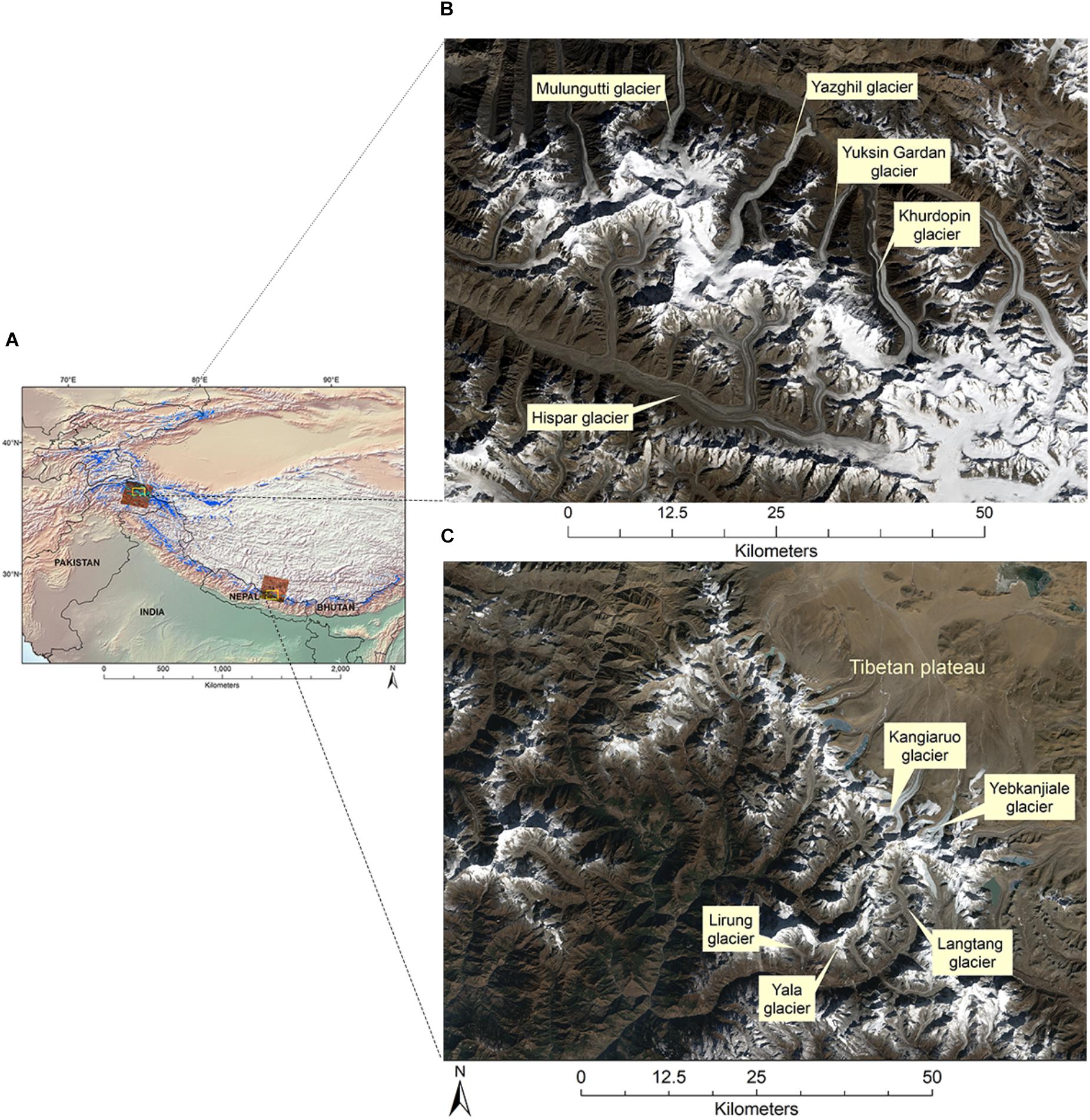
Figure 1. Study area with the two subset regions investigated: (A) location map showing High Mountain Asia and the two subset areas, with the glacier outlines (in blue) from the Randolph Glacier Inventory (Pfeffer et al., 2014) and background shaded from Natural Earth; (B) part of the Hunza basin (Shimshal Valley) in Western Himalaya, Northern Pakistan; and (C) part of the Trishuli basin in Central Himalaya, Nepal. Snowlines are well visible on (B) and (C) Landsat 8 true color composites (bands 4, 3, and 2) acquired late in the year (November and December), respectively.

The second study area is part of the Narayani basin the Central-Eastern Himalaya of Nepal (Figure 1C). Climatically, this region is influenced by the south-west Asian summer monsoon circulation system (Yanai et al., 1992; Benn and Owen, 1998). Moist air masses from the Bay of Bengal interact with the topography of the Himalaya and Tibetan Plateau (HTP), causing maximum precipitation on the southern slopes of the Himalaya during the summer months (June–September) (Shrestha, 2000; Bookhagen and Burbank, 2006). Glaciers in this monsoon-influenced part of the Himalaya are of “summer-accumulation” type (Ageta and Higuchi, 1984; Thayyen and Gergan, 2010). The headwaters of glaciers in the Trishuli basin originate from China; our study area spans both the southern and the northern slopes of the Himalaya (Figure 1C). ELA measurements are scarce in this area as well, and most estimates come from indirect methods (Kayastha and Harrison, 2008) or modeling approaches (Acharya and Kayastha, 2019).

Data Sources

The main satellite data sources for this study are from the Landsat 7 Enhanced Thematic Mapper (ETM +) and the Landsat 8 Operational Land Imager (OLI) and Thermal Infrared Sensor (TIRS), obtained from the USGS. These two sensors have been acquiring imagery in the visible, near infrared, short wave infrared and thermal bands of the electromagnetic spectrum since 1999 and 2013, respectively [see USGS (2016) for more details]. Monthly Landsat OLI scenes from 2013 (for Hunza) and 2016 (for Trishuli) were used to determine seasonal SLAs fluctuations and to estimate the approximate date of end-of-ablation season in each region (Table 1). The years were selected based on maximum number of cloud-free images with good contrast over snow and ice in each area. The year 2013 had snowy and cloudy conditions in the Trishuli, making it hard to obtain suitable images, so we could not use the same year as for the Hunza for the seasonal analysis. Annual Landsat ETM+ scenes (2000–2012) and OLI (2013 and 2016) were used to map ELAs and to assess ELA fluctuations over the 16-year record. These scenes were selected using a 4-month window in each area (August–October for the Hunza and September–December for the Trishuli) based on the seasonal SLAs and on previous literature (Thayyen and Gergan, 2010). We used digital numbers (DNs) rather than atmospheric reflectance since the latter was not available at the onset of our study.

TABLE 1

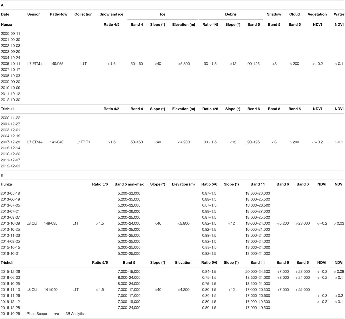
Table 1. Landsat 7 ETM+ and Landsat 8 OLI remote sensing data used in this study, with the optimized thresholds applied to band ratios and topographic criteria to partition the snow, ice, and debris surfaces. DN ranges represent the (minimum and maximum) values used to map ice and debris cover. Thresholds were used for: A: annual analysis (2000–2016) and B: seasonal analysis (2013 for the Hunza and 2016 for the Trishuli).

To extract SLAs, we used elevations from the Shuttle Radar Topography Mission (SRTM), which acquired near-global data in February 2000. We used two SRTM versions: (a) the hydrologically sound, void-filled SRTM DEM from the Consultative Group for International Agriculture Research Consortium for Spatial Information (CGIAR-CSI version 4.1) at 3-arc seconds (∼90 m); this dataset was released in 2008 (Jarvis et al., 2008), with void-filling procedures described in Reuter et al. (2007) and (b) the NASA SRTM Version 3.0 (SRTMGL1), at 1-arc second (∼30 m); this was released in 2015 and was void-filled using elevation data mostly from the Advanced Spaceborne Thermal Emission and Reflection Radiometer (ASTER) Global Digital Elevation Model 2 (GDEM2) (NASA-JPL, 2013). The SRTM global DEM targeted a vertical accuracy of ±16 m (Rabus et al., 2003) but in rugged terrain, accuracy can be considerably lower (Berthier et al., 2006; Fujita et al., 2008). In a recent study, Mukul et al. (2017) evaluated the 90 and 30 m versions of the SRTM DEMs and reported an uncertainty (as vertical root mean square error, RMSE_z) of 47.2 and 23.5 m, respectively, based on ground control points in the Himalaya. Bias correction improved the accuracy of both of these DEMs in the cited study. In our study, we accounted for DEM errors in our SLA/ELAs on the basis of the uncertainties reported by Mukul et al. (2017).

Surface Partitioning: Clean Glacier Ice, Snow on Ice, Snow on Land, and Debris Cover

The various snow-ice-debris surfaces were separated using a multi-criteria method implemented in Python as a series of conditional statements, based on band ratios and topographic criteria. Thresholds for various band ratios, elevation, slope, and temperature criteria were selected based on visual inspection of Landsat color composites, previous literature and a priori knowledge. Thresholds for the monthly series were adjusted since they varied seasonally; thresholds for the annual time series were standardized for all images. The criteria used, along with their thresholds, are reported in Table 1; an overview of the surface partition process is presented in Figure 2. The output of surface partition algorithm was a four-class raster when no seasonal snow was present (Figures 2A,B) or a five-class raster for the months when seasonal snow was present.

FIGURE 2

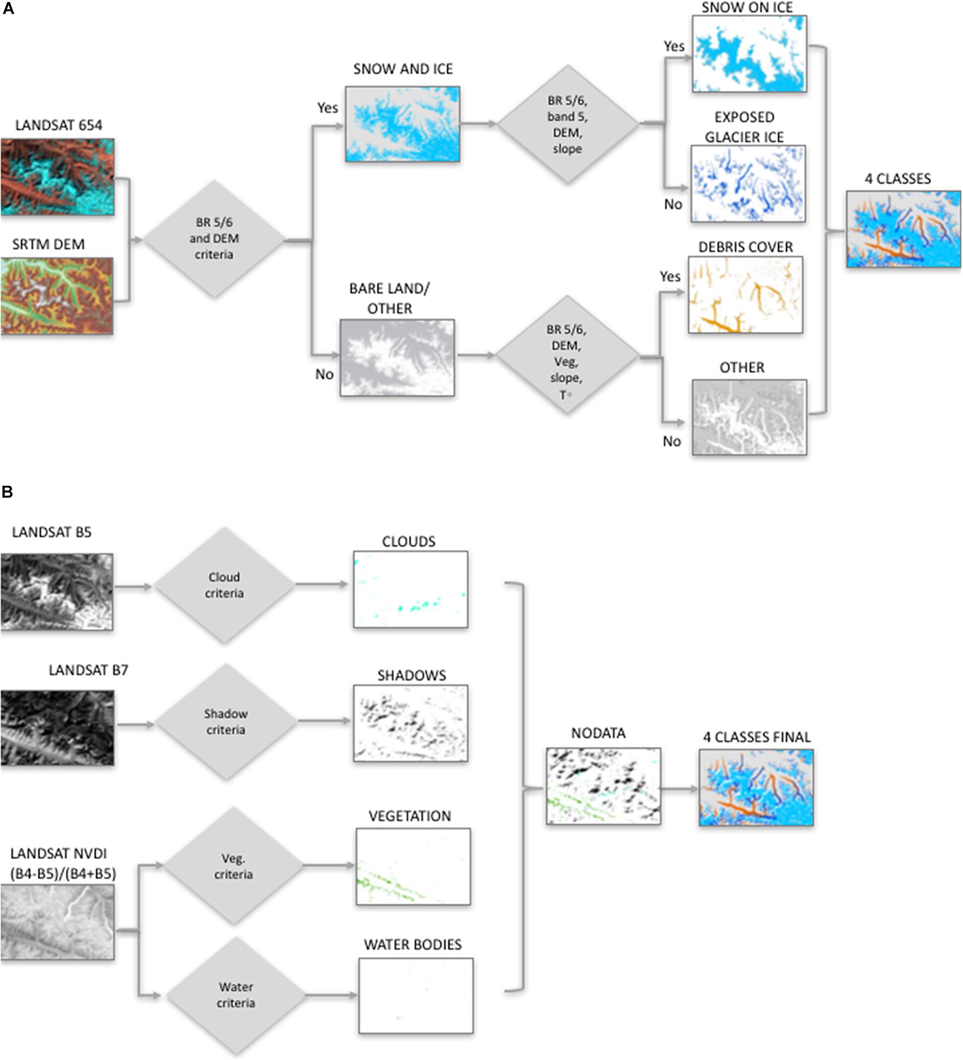
Figure 2. Surface partition workflow using Landsat bands and a DEM, and its outputs: (A) band ratios for separating exposed glacier ice, snow on ice and debris covered ice from bare land; and (B) band ratios for delineating clouds, shadows, vegetation, and water bodies.

In a preliminary step, we used single band ratios to mask areas under shadow, clouds, and surface water, which pose challenges for the semi-automated band ratio methods (Racoviteanu et al., 2009). Deep shadows are common in mountainous areas on steep slopes especially in the winter due to the low sun angles in the morning around the time of acquisition of the Landsat scenes (∼05:36 GMT or ∼10:36 local time for this particular area). Shadows appear darker than other surfaces in the near-infrared, so we used this wavelength to map shadows from steep terrain, including cast shadow from clouds, which are also an issue (Racoviteanu and Williams, 2012). We applied a threshold to band 5 (ETM+) or band 6 (OLI), which we checked and adjusted for each month in the time series to obtain shadow “masks.” Tests for the cloud mapping techniques based on the FMask algorithm (Zhu et al., 2015; Zhu and Helmer, 2018) failed to distinguish between snow and clouds in this area. Therefore, in this study, clouds were mapped using a single band threshold. At near infrared (ETM+ band 5: 1.55–1.75 μm) and shortwave infrared wavelengths (OLI band 6: 1.57–1.65 μm), snow and ice surfaces are dark and clouds are bright, making these two types of surfaces distinguishable. We carefully adjusted the DN thresholds to avoid misclassifying illuminated bare terrain as clouds (Table 1), even though we consider that this would have little/no effect on our surface classifications. Shadow and cloud raster masks were assigned “NoData” values in the final maps (Figure 2B). Vegetated areas were mapped using the Normalized Difference Vegetation Index (NDVI), defined here as the difference between visible and near infrared bands, i.e.,

$${\text{NDVI}}_{\text{TM}}=\mathrm{}{\displaystyle \frac{\mathrm{band}\mathrm{\hspace{0.33em}3}-\mathrm{band}\mathrm{\hspace{0.33em}4}}{\mathrm{band}\mathrm{\hspace{0.33em}3}+\mathrm{band}\mathrm{\hspace{0.33em}4}}}\text{and} {\text{NDVI}}_{\text{OLI}}=\mathrm{}{\displaystyle \frac{\mathrm{band}\mathrm{\hspace{0.33em}4}-\mathrm{band}\mathrm{\hspace{0.33em}5}}{\mathrm{band}\mathrm{\hspace{0.33em}4}+\mathrm{band}\mathrm{\hspace{0.33em}5}}}(1)$$

The NDVI algorithm results in a raster with values from −1 to 1. This was used to map both the vegetation areas (negative values) and water bodies (positive values) (Table 1), which were excluded from the potential debris cover map and assigned to the “bare land” class. Mapping the water bodies (lakes and rivers) was only introduced in the Trishuli subset as an improvement of the method, though this did not affect the surface partition on glaciers.

Glacierized areas (clean glacier ice and snow) were mapped using the standard semi-automated “band ratio” technique, which is robust and easy to apply over large areas, and widely used by the glaciological community (Racoviteanu et al., 2009; Bolch et al., 2010; Paul et al., 2013). This technique takes advantage of the spectral difference between snow and ice surfaces and other types of terrain in the visible and near-infrared parts of the electromagnetic spectrum. We calculated the ratio of DNs using two bands ($\frac{\mathrm{band}\mathrm{\hspace{0.33em}4}}{\mathrm{band}\mathrm{\hspace{0.33em}5}}$ for ETM+ and $\frac{\mathrm{band}\mathrm{\hspace{0.33em}5}}{\mathrm{band}\mathrm{\hspace{0.33em}6}}$ for OLI) and thresholded the resulting raster to obtain a binary map (1 = “snow/ice,” 0 = “other”) (Figure 2A). The segmentation of band ratio images using raw DNs has been found to be superior over band ratios using atmospherically corrected images when cast shadow was present (Paul et al., 2002). We used a band ratio threshold of 1.5 for all our images (Table 1). We tested various thresholds from the literature (1.2–2) on the basis of false Landsat color composites (ETM+ bands 5, 4, 3 and OLI bands 6, 5, and 3) and we conducted a sensitivity analysis to these thresholds (section “Sensitivity Analysis”). The lower threshold of 1.5 compared to the ones used for glacier mapping (Andreassen et al., 2008; Racoviteanu et al., 2015) allowed mapping the full extent of snow and ice for each time step. The minimum snow and ice area for any given year (2013 for Hunza, 2016 for Trishuli) was considered to represent the glacier surface for that year and was used as a “glacier mask” for the subsequent steps described below.

Snow on ice in the accumulation area of glaciers was separated from exposed glacier ice in the ablation area by thresholding the near-infrared band (ETM+ band 4 at 0.77–0.90 μm and OLI band 5 at 0.851–0.879 μm), along with an elevation and a slope criteria (Figure 2A). At these wavelengths, ice and snow have different brightness temperatures, making them distinguishable from each other. Due to differences in illumination conditions, the thresholds varied depending on each image. To pick a threshold, for OLI band 5, for example we defined regions of interest (ROI) on exposed glacier ice surfaces and extracted summary statistics from OLI band 5 over 1 year. On the basis of mean statistics, we tested various thresholds to compute an “optimized” ratio for each month, which was adjusted for each time step based on visual inspection (Table 1). The sensitivity of the resulting SLAs to these thresholds will be discussed later (section “Sensitivity Analysis”). We concurrently applied a slope criterion (ice <40°) and an elevation criterion (ice >2,800 m a.s.l. for the Hunza and ice >4,200 m a.s.l. for the Trishuli) to further constrain the clean ice class, i.e., to exclude steep slopes (rock) and lower elevations (illuminated moraines and bright surface water) from the snow/ice class. The slope thresholds are consistent with previous studies in the Hunza (Hewitt, 2011; Khan et al., 2015), where slopes >35° represent internal rocks in the accumulation area of glaciers. Based on visual interpretation, here we chose a maximum value of 40° to constrain the ice class. The outcomes of this step were clean ice and snow on ice classes.

Debris covered ice was mapped by thresholding the band ratio (ETM+ 4/5, OLI 5/6), a slope derived from the DEM, a thermal band (ETM+ band 6, OLI band 11) and an elevation layer. Each threshold was adjusted for each image on the basis of the visual interpretation of color composites; these are reported in Table 1. The thresholds for slope and thermal band were based on previous research (Racoviteanu and Williams, 2012). Minimum and maximum values of thermal bands were adjusted based on visual interpretation; these are generally lower in the fall or winter months, when debris covered ice surfaces are cooler due to less solar heating and lower temperatures, but they vary due to different illumination conditions. Only the exposed (snow-free) part of the debris covered ice was mapped in this step.

Snow on land was estimated for each image using the minimum snow and ice area, i.e., the “glacier mask” described in this section. For any given time step, when the extent of snow and ice was larger than the initial glacier mask area, the additional pixels were classified as seasonal snow and output as snow on land. For the purposes of parameterizing the melt model used in Armstrong et al. (2019), any snow present on the surface of debris covered tongues was also mapped and referred to as snow or land. We performed post-classification corrections to adjust misclassified areas, which included: (a) some glacier edges misclassified as snow as a result of the mixed spectra from glacier ice and rock; (b) shadows in the accumulation areas of glaciers which have a similar spectral signature to ice and were misclassified as exposed glacier ice; and (c) bare illuminated terrain misclassified as debris covered ice. Manual corrections were applied only to the subset study areas for purposes of conducting a sensitivity analysis to manual corrections.

Misclassified areas from (a) and (c) were adjusted manually, with only minimal processing of debris cover, which was not the focus here. Shadows misclassified as ice (b) were corrected automatically by creating a negative buffer (−2,000 m) inside the full glacier ice and snow mask, i.e., “shrinking” the mask. The false snowlines located within the shrunken mask were “erased” automatically with an overlay vector operation for all dates, thus reducing the time needed for manual edits. We refer to the resulting versions over subset areas as “corrected” and the raw, full extent versions as “uncorrected.”

Automated Snowline Extraction: The “Buffer” Method

Snowlines were extracted in an automated way using a buffer applied to the snow and ice areas obtained from the surface partition at each time step (Figures 3A–H). Buffers have been used to extract snowline elevations in the Central Himalaya (Garg et al., 2017) or to estimate uncertainties in mapped glacier area in the Cascades (Granshaw and Fountain, 2017). While Garg et al. (2017) extracted snowlines only over the centerline of glaciers, here we estimated snowlines over the full extent of glaciers. Furthermore, while Garg et al. (2017) fixed the buffer size to 30 m around manually delineated snow areas, in this study we adapted the buffer size to the two DEMs tested (50-m buffer size for the 90-m CGIAR, and a 15-m buffer for the 30 m SRTMGL1). We performed a sensitivity analysis to the DEM and the buffer size used (section “Sensitivity Analysis”). For each time step, we intersected snow buffers to obtain a snowline interval, and then extracted elevations on a pixel-by-pixel basis from the DEM to obtain snowline elevations (Figure 3). Pixel-by-pixel SLA values are sensitive to outliers, so we estimated regional SLAs as the median elevation within the buffer interval over the full or subset image. Using the median rather than the mean accounts for non-normally distributed data in some of the months. The maximum SLA in a given year was considered the ELA for that year (Figure 3). SLAs were output automatically in tables, along with the ID of the scene and the parameters used for each run.

FIGURE 3

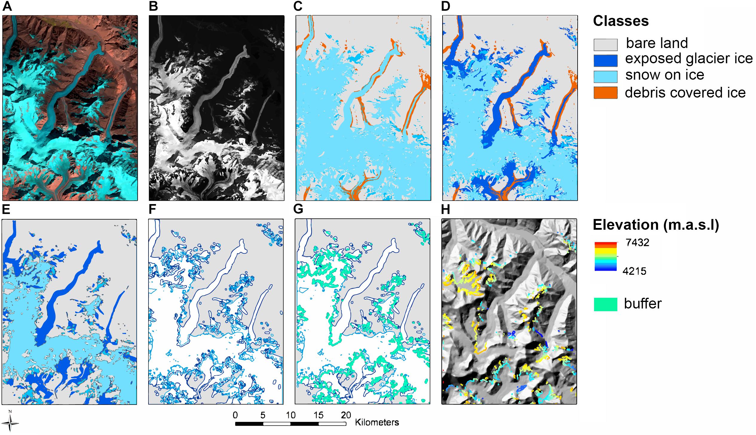
Figure 3. Intermediate products from the buffer method used in extracting the snowlines from Landsat images. Here we show an example from the Hunza: (A) false color composite (bands 6, 5, 4); (B) band 5; (C) separating ice and snow from debris covered ice; (D) separating snow on ice, clean ice, debris cover, and bare land; (E) extracting clean ice vs. snow on ice; (F) converting raster to ice and snow polygons, buffering the polygons and intersecting the polygons; (G) extracting the buffer polygon; and (H) extracting the elevation of pixels inside the buffer.

Uncertainty Estimates

Snow and ice mapping derived from remote sensing are subject to uncertainties issued from image classification techniques, mixed pixels and internal rocks, as discussed in previous studies (Racoviteanu et al., 2009; Paul et al., 2013). In this study, we used a standardized band ratio method to distinguish snow and ice from surrounding terrain, with carefully chosen thresholds. On the basis of previous studies (Paul et al., 2013), the accuracy of the glacier outlines derived from remote sensing using the automated technique is estimated as ± 1 pixel size (30 m). Multiple digitizing experiments have also found the accuracy of the automated glacier outlines to be within the variability of those obtained by manual digitization (Paul et al., 2013). Since here we only mapped the entire ice masses, and intersected them to get snowlines, we are not reporting the glacier outline accuracy directly, but we rather focus on the snowline accuracy.

Sources of uncertainty in the SLA estimates come from: (1) the accuracy of the DEM used for the surface partition (90 m CGIAR and 30 m SRTMGL1); (2) the size of the buffer used to extract the snowlines; (3) uncertainty in snow and ice area estimates; and (4) overall uncertainties in the automated method used to partition the surfaces. These were defined and estimated as follows:

• ε_dem is the vertical error of the SRTM DEM (RMSE_z), defined as 47.2 m for the 90 m CGIAR DEM and ± 23.5 m for the 30 m SRTMGL1 DEM based on Mukul et al. (2017).

• ε_buffer represents the buffer size used for the snowline extraction, defined as ±15 m for the 30 m SRTMGL1 and ±50 m for CGIAR (see section “Automated Snowline Extraction: The ‘Buffer’ Method”).

• ε_outlines is considered to be 1/2 of the pixel size of the Landsat satellite imagery used, i.e., ±15 m. We consider this error to be embedded in the buffer size of ±15 and ±50 m.

• ε_edit is related to uncertainties in the algorithm itself, which varies with each image and is related to the choice of band ratios thresholds and elevation criteria chosen for each time step. We quantified this error as the difference in SLAs resulting from the uncorrected (raw) and corrected (manually edited) versions of the surface partition for each time step (see section “Surface Partitioning: Clean Glacier Ice, Snow on Ice, Snow on Land and Debris Cover”).

Assuming that the individual sources of error are uncorrelated, we estimated SLA accuracy as root mean square error (RMSE_z) for the uncorrected and corrected versions. For the snowlines issued from the uncorrected versions (full and subset extents), the total error (ε_uncorr) is:

$${\text{ε}}_{\text{uncorr}}=\sqrt{{\text{ε}}_{\text{dem}}^2+{\mathrm{\epsilon }}_{\text{buffer}}^2+{\mathrm{\epsilon }}_{\text{edit}}^2}(2)$$

For the snowlines issued from manually corrected surface partitions, the total error (ε_corr) is:

$${\text{ε}}_{\text{corr}}=\sqrt{{\text{ε}}_{\text{dem}}^2+{\mathrm{\epsilon }}_{\text{buffer}}^2}(3)$$

Snowline Validation

We validated the snowlines in one of our study areas (Trishuli), where PlanetScope high-resolution imagery was available for the same date as the Landsat OLI scene (October 25, 2016) (Planet_Team, 2017). There were no Planet scenes available for the Hunza area, so we could not perform a similar validation there. The PlanetScope sensor acquires data at visible to near-infrared wavelengths (four bands), with a swath width of 24.6 × 16.4 km and 3 m ground resolution. PlanetScope provides image stripes of orthorectified, Top of Atmosphere radiance (at sensor), as analysis-ready data. Image stripes were combined in a single mosaic and bands 4, 3, and 2 were used to create false color composites. We manually digitized a total of 32 visible snowlines as vectors on the PlanetScope image using these color composites for individual glaciers from RGI. We rasterized the lines and extracted elevations along each digitized line based on the SRTMGL1 DEM (30 m), and averaged these to obtain PlanetScope SLAs for each glacier. Given the DEM cell size, a 15 m buffer is automatically embedded in the calculation of PlanetScope SLAs. We compared the OLI-based SLAs with those derived from PlanetScope using parametric statistical tests and basic statistics.

Results

Monthly Surface Partition: Hunza (2013) and Trishuli (2016)

Here we present the monthly fluctuations of the various surfaces for Hunza (May–December 2013) (Figure 4) and Trishuli (June–December 2016) (Figure 5). The areas of “NoData” represent shadows and clouds; while most images are cloud-free over glaciers, deep shadows get progressively larger in the winter (November through December) in both areas due to low sun angles and the effect of rugged terrain. Clouds are more prevalent in the Trishuli, especially during the months of October to December. In Table 2 and Figure 6 we present summaries of total area for surfaces on the glacier and off-glacier in the subset areas (Hunza and Trishuli). In both areas, as snow decreases, exposed glacier ice increases. For example, for the Hunza subset in 2013, the exposed glacier ice increased from a minimum of 4.5% of the glacierized area on May 18 to a maximum of 24.1% of the glacierized area on October 9, and then decreased again to 6.2% in November after snowfall (Table 2). These seasonal fluctuation patterns are visible in Figure 4, which shows glacier ice progressively being exposed as the season progresses until October 9, and then snow on land increasing to a maximum on November 26. The same patterns are visible in the Trishuli (Figure 5). In the winter months, almost no exposed glacier ice is visible over the entire extent (Figures 4, 5). In the Trishuli, the exposed glacier ice increased from a minimum of 4.7% of the glacierized area on June 3 to a maximum of 26.8% on December 12, 2016, which was the maximum for this particular year (Table 2 and Figure 6). Minimum exposed glacier ice occurred roughly around the same time of the year (May–June) for both areas, but the maximum occurred later in the season in the Trishuli (December 2016) compared to the Hunza (October 2013) for the years studied (Table 2). In the Trishuli, the total glacierized area exhibited an apparent decline by about 200 km² in exposed glacier ice from spring to winter in 2013; however, this was due to a large number of NoData values due to clouds or shadows obscuring the glacier surface during winter season in this area, and was not a “true” glacier ice loss.

FIGURE 4

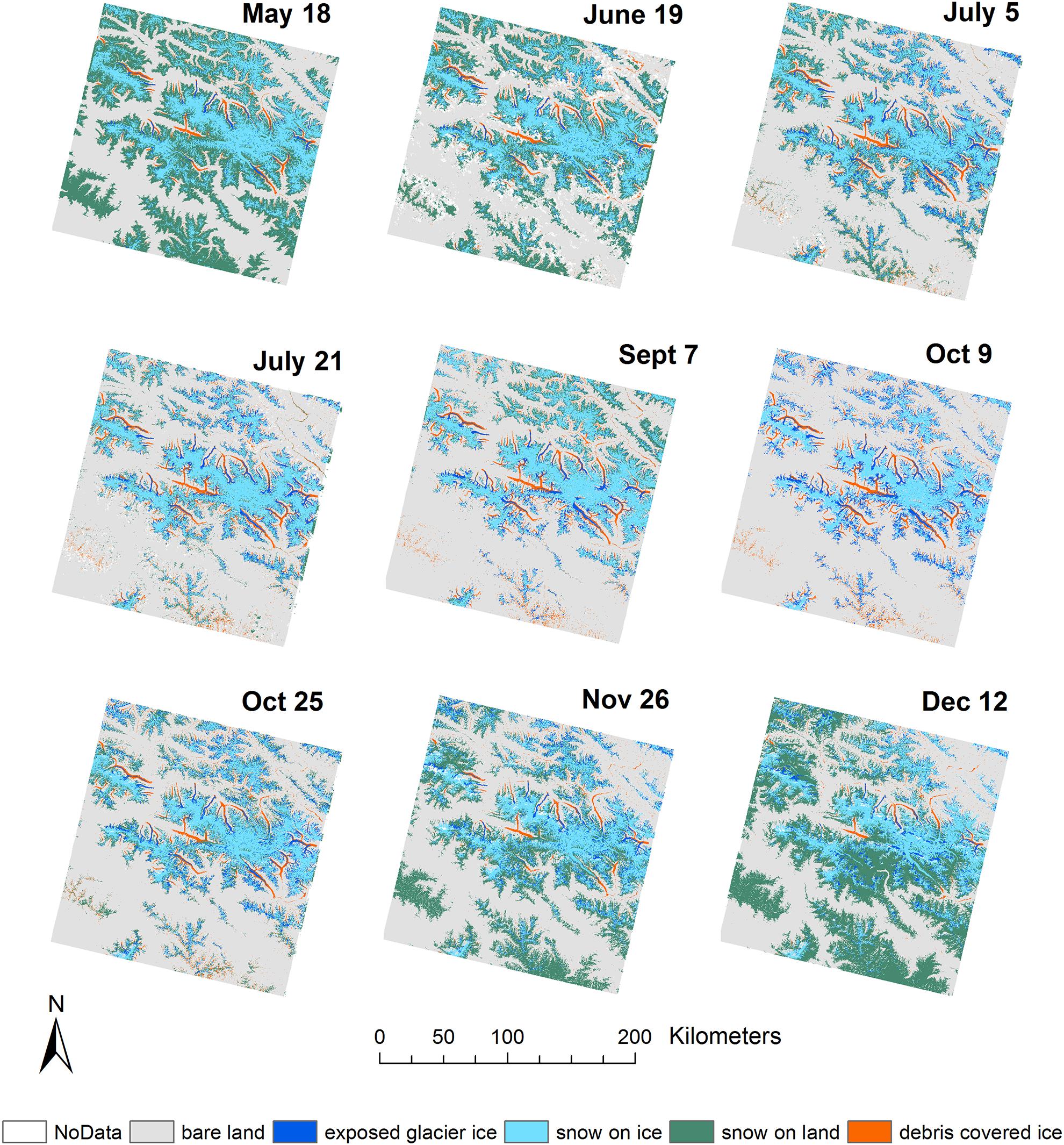
Figure 4. Time series of the monthly partition of the snow, ice and debris surfaces for the full extent of the Hunza (May–October 2013) using raw, uncorrected outputs based on the 90 m CGIAR. Seasonal snow on land increases toward December when there is almost no exposed glacier ice visible. Some topographic shadows in the accumulation areas are mis-classified as glacier ice, needing manual correction.

FIGURE 5

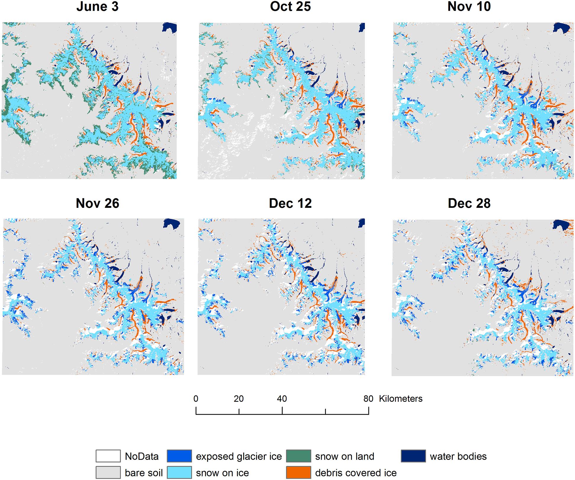
Figure 5. Time series of the monthly partition of the snow, ice and debris surfaces for the subset extent of the Trishuli where glaciers are located (June–December 2016). The water bodies are shown in dark blue for reference but are not discussed in the text.

TABLE 2

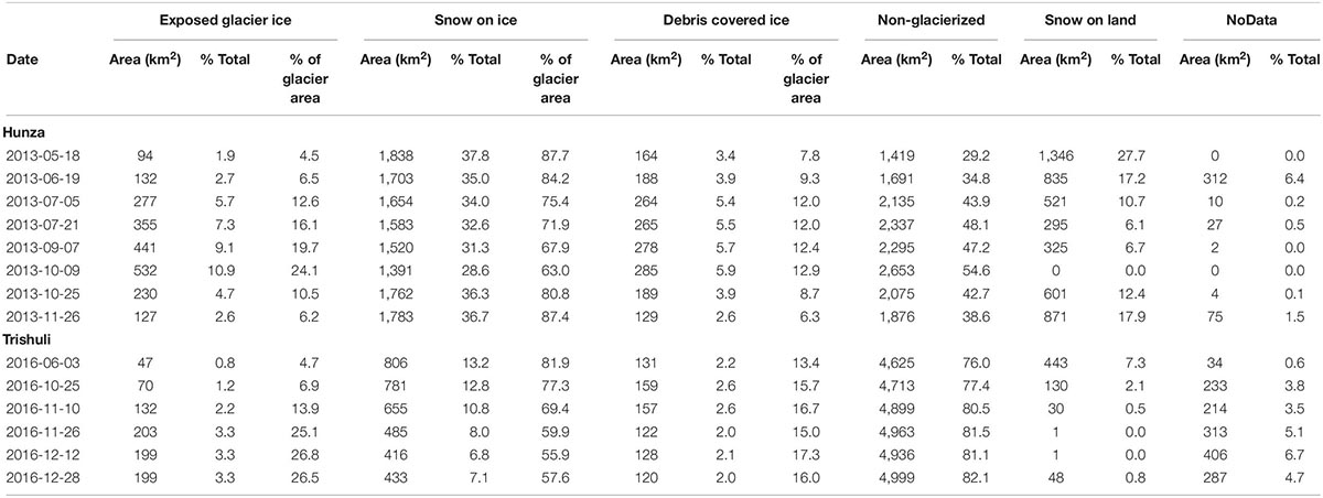
Table 2. Monthly surface partition for the Hunza and Langtang subset areas for 2013 and 2016, respectively, after the manual corrections. NoData refers to areas under clouds or shadow. The NGL class includes water bodies (Trishuli only). The areas occupied by non-glacierized (bare) terrain are reported for reference, but are not discussed here.

FIGURE 6

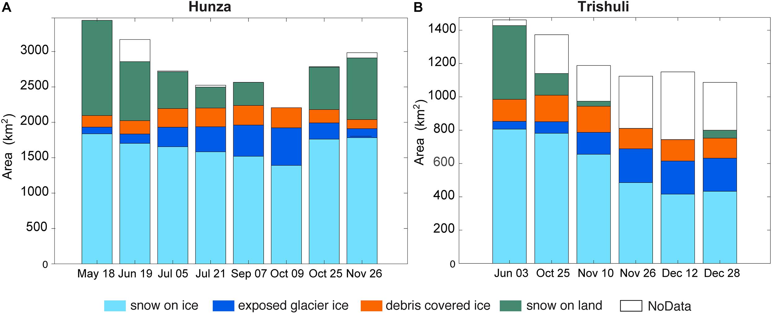
Figure 6. Summarized areas for each month for snow on ice, exposed glacier ice, debris covered ice snow on land, and NoData: (A) Hunza and (B) Trishuli.

Snow on ice in the Hunza decreased from a maximum of 87.7% of the glacierized area on May 18 to a minimum of 63.0% of the glacier area on October 9, when maximum glacier ice was exposed and then increased again to 87.4% on November 26 (Table 2). In the Trishuli, snow on ice decreased from 81.9% of the glacierized area on June 3 to 55.9% on December 12 (Table 2 and Figure 6) and then increased slightly to 57.6%. The debris covered ice area showed little variability, since debris cover is not expected to change significantly throughout the year (Table 2). Debris covered surfaces were being progressively exposed as snow at the debris surface melted (Figure 6). Since the snow on land class includes snow on debris as well, the debris covered ice area fluctuation was not a true surface area change. In the Hunza, the debris covered ice area ranged from a minimum of 7.8% of the study area in the spring, when part of the debris covered glacier tongues were covered by snow, to a maximum of 12.9% on October 9 after all snow had melted. Similarly, for the Trishuli, debris cover extent ranged from a minimum of 13.4% on June 3 to a maximum of 17.3% on December 12 (Table 2).

Outside the glacierized area, snow on land fluctuated from 27.7% of the total subset area in the Hunza on May 18 to a minimum of 0.0% on October 9 in the Hunza and from 7.3% of the total subset area in Trishuli in June to 0.01% on November 26 and December 12. Snow outside glaciers diminished as the melt season progressed, as expected (Table 2 and Figure 6).

Monthly Snowline Fluctuation in the Hunza (2013) and Trishuli (2016)

In the subset area of Hunza (Shimshal valley), the automated surface partition with manual corrections yielded the lowest SLA of 4,727 ± 69 m a.s.l. on May 18 and the highest SLA of 5,171 ± 69 m a.s.l. on October 9 (Table 3 and Figure 7A). After this date, SLA decreased in late fall/winter, which is consistent with the increase in seasonal snow in November and December (Table 2). The date of highest SLA in the Hunza coincides with the maximum exposed glacier ice on October 9, and therefore we consider this date to be the end of the ablation season in 2013 in this area. This is in general agreement with Minora et al. (2016), who used the Julian day 273 or nearby date as an indicator of the end-of-the-summer SLA in their remote sensing study of glaciers from 2001 to 2011 in the Central Karakoram in northern Pakistan. By contrast, a previous study (Khan et al., 2015) had used July—August as the window of time to estimate maximum SLA for the Hunza, which is earlier than our findings.

TABLE 3

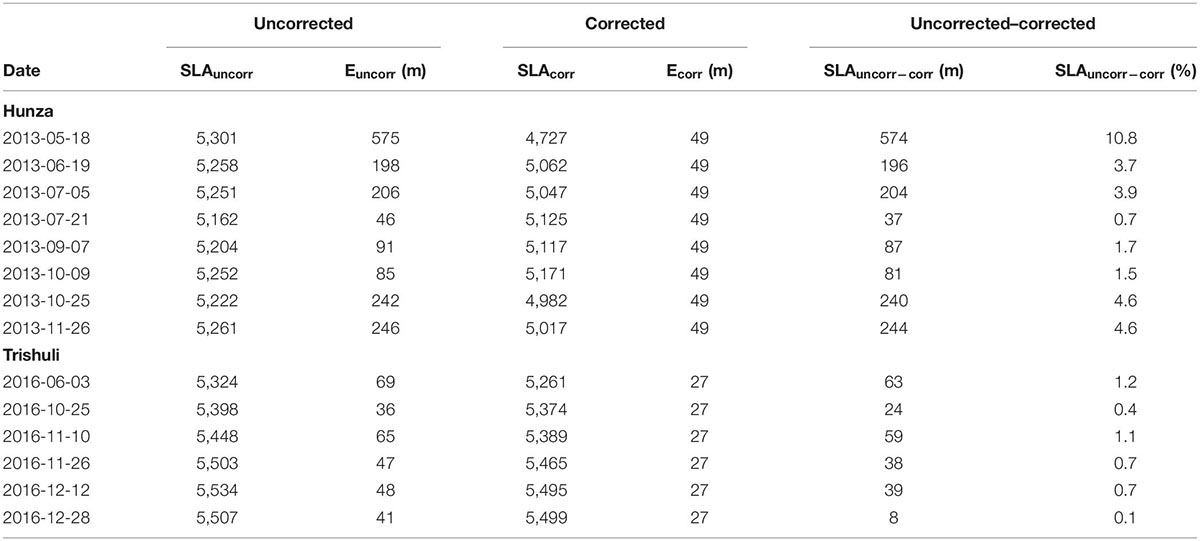
Table 3. Snowline altitudes for the Hunza and Trishuli subset extents obtained from the “uncorrected” and “corrected” versions of the partitioning, using the SRTMGL1 (30 m) and a 15-m buffer. Here, we refer to SLAs as median of all pixels classified as SLA for the subset and full extent of Landsat. Respective error estimates E uncorr and Ecorr represent RMSEz (see section Uncertainty estimates). Manual corrections of the surface partitioning had the biggest impact on the resulting SLAs for the spring and late fall months, particularly in the Hunza study area where the errors were the largest.

FIGURE 7

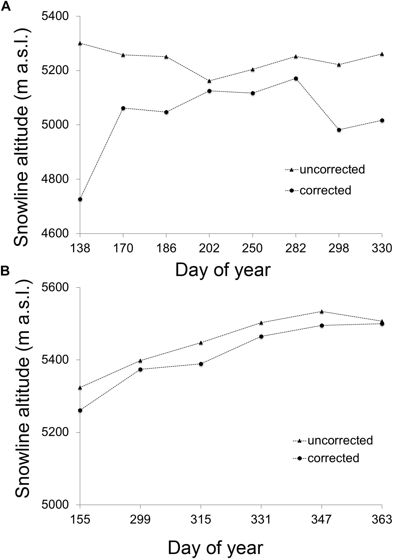
Figure 7. Monthly SLAs before and after the manual corrections applied to the surface partition in the subset extents for: (A) Hunza and (B) Trishuli.

For the Trishuli, manual corrections of the surface partition yielded the lowest SLA of 5,261 ± 27 m a.s.l. on June 3, and the highest SLAs of 5,495 ± 27 m a.s.l. on December 12, and 5,499 ± 27 m a.s.l. on December 28 (Table 3 and Figure 7B). Since on the December 28 image we detected some seasonal snow (0.8%) (Table 2 and Figure 6), we consider December 12 to be the end of the ablation season for 2016.

The month marking the end of the ablation season was different in the two regions. In the Hunza, the highest SLA in 2013 occurred in October, versus in December in Trishuli in 2016. We cannot elaborate on the potential causes but we speculate that this later-than-usual highest SLA in the Trishuli could be linked with increased summer air temperature trends as noted in the Nepal Himalaya (Fujita and Nuimura, 2011), and potentially drier conditions in 2016. The temporal frequency of images from Landsat does not allow us to determine the precise day of the highest SLA, only the month.

Annual ELAs in the Hunza and Trishuli (2000–2016)

Annual ELAs extracted from images from the end-of-ablation season date established above (October-November) (Figure 8) show little variability from year to year from 2000 to 2016 in both areas (on average within ± 100 roughly with a few exceptions), indicating somewhat stable glacier conditions. In the Hunza, annual ELAs ranged from 5,142 ± 100 m a.s.l. in 2009 to 5,228 ± 97 m a.s.l. in 2013, with an average of 5,176 ± 100 m a.s.l. over the entire period (2000–2016). This is in general agreement with other ELA estimates in the Karakoram for the same time period, for example Minora et al. (2016), who reported an average ELA of ∼ 5,200 to 5,300 m a.s.l. for the 2001–2010 period in Central Karakoram based on Landsat images; they assumed Julian day 273 or nearest date as the reference for the end of summer. Since they reported the ELA as a single elevation over the entire period, we cannot compare our results with theirs at annual time steps. Our ELA estimates are lower than those of Kääb et al. (2012) (ELA: 5,540 m a.s.l.) for the Karakoram region based on Landsat scenes.

FIGURE 8

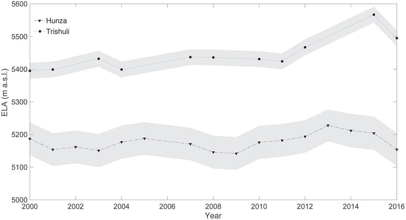
Figure 8. Annual ELAs in the Hunza and Trishuli from 2000 to 2016, based on surface partition using the SRTMGL1 DEM (30 m) with a 15 m buffer. ELAs are expressed as the maximum snowline altitude (SLA) of each year. Error intervals are shown as ±1/2 of the RMSEz of total uncertainties (see section “Uncertainty Estimates”).

In the Trishuli, annual ELAs varied from a minimum of 5,395 ± 48 m a.s.l. in 2000 to a maximum of 5,567 ± 48 m a.s.l. in 2016, with an average of 5,444 ± 48 m a.s.l. over the entire period (2000–2016). This is in close agreement with regional ELAs of ∼5,400 m a.s.l. used in recent hydrologic studies in the same area (Ragettli et al., 2015). In a previous study, we estimated mean ELA values of 5,468 m a.s.l. in 2003 based on manual digitization on ASTER imagery (Racoviteanu et al., 2013). In the present study, we obtained an ELA of 5,432 m a.s.l. for the same year (2003), in close agreement with the previous value. Regional ELAs estimated in the current study for 2011 and 2012 (5,424 and 5,467 m a.s.l.) are also in agreement with ELA values reported in Acharya and Kayastha (2019) for the Yala glacier (5,441 and 5,412 m a.s.l., respectively). The higher annual ELAs in 2015 and 2016 in the Trishuli (ELA: 5,567 and 5,495 m a.s.l., respectively) (Figure 8) are in agreement with Acharya and Kayastha (2019) (ELA: 5,451 m.a.s.l.; ELA: 5,555 m.a.s.l), explained by more negative summer mass balance conditions in the cited study. A careful assessment of the 2015 ELA showed no bias or significant errors, so we speculate that the higher ELAs in 2015 and 2016 may be linked with local climatic conditions. Huss and Hock (2015) used a single ELA value of 5,215 m a.s.l. for southwest Asia for their model and projected a rise in the regionally average glacier ELAs by 100 to 500 m from 2010 to 2100. Due to the time scale of our analysis (2000–2016) and the lack of a clear temporal upward trend in ELA, we cannot make any statements with regards to the suggested trends in the cited study. On the contrary, for the Hunza, our results imply relatively stable conditions, in agreement with cooling trends in summer temperature noted in the last decade (Forsythe et al., 2017).

Comparison With SLAs From High Resolution Imagery

In the Trishuli, the comparison between semi-automated (Landsat 8 OLI) vs. manual (PlanetScope) SLAs (Figure 9) yielded an average difference of 41 m, with a standard deviation of 64 m and a RMSEz of 137 m. SLA values obtained from Landsat and Planet had equal variances based on an F-test at 95% confidence interval. The mean SLA values from PlanetScope (5,301 m a.s.l.) vs. Landsat OLI (5,258 m a.s.l.) were not statistically different based on the t-test for two sample assuming equal variances. On a glacier-by-glacier basis, differences in Planet vs. Landsat SLAs ranged from −53 m (overestimated) to +240 m (under-estimated). In general, the semi-automated algorithm using Landsat 8 OLI underestimated most SLAs compared to PlanetScope, but results show good agreement (R² = 0.95) (Figure 9). The underestimation in OLI SLAs is due to the presence of brighter pixels or old snow in the lower ablation area of glaciers. Due to the similarly spectral signal of these ice pixels to snow, the algorithm detects an ice-snow boundary and classifies these pixels as part of the snowlines. Since these patches are situated at lower altitudes, these misclassified pixels introduce negative biases in the SLA estimates, and they need to be filtered out manually.

FIGURE 9

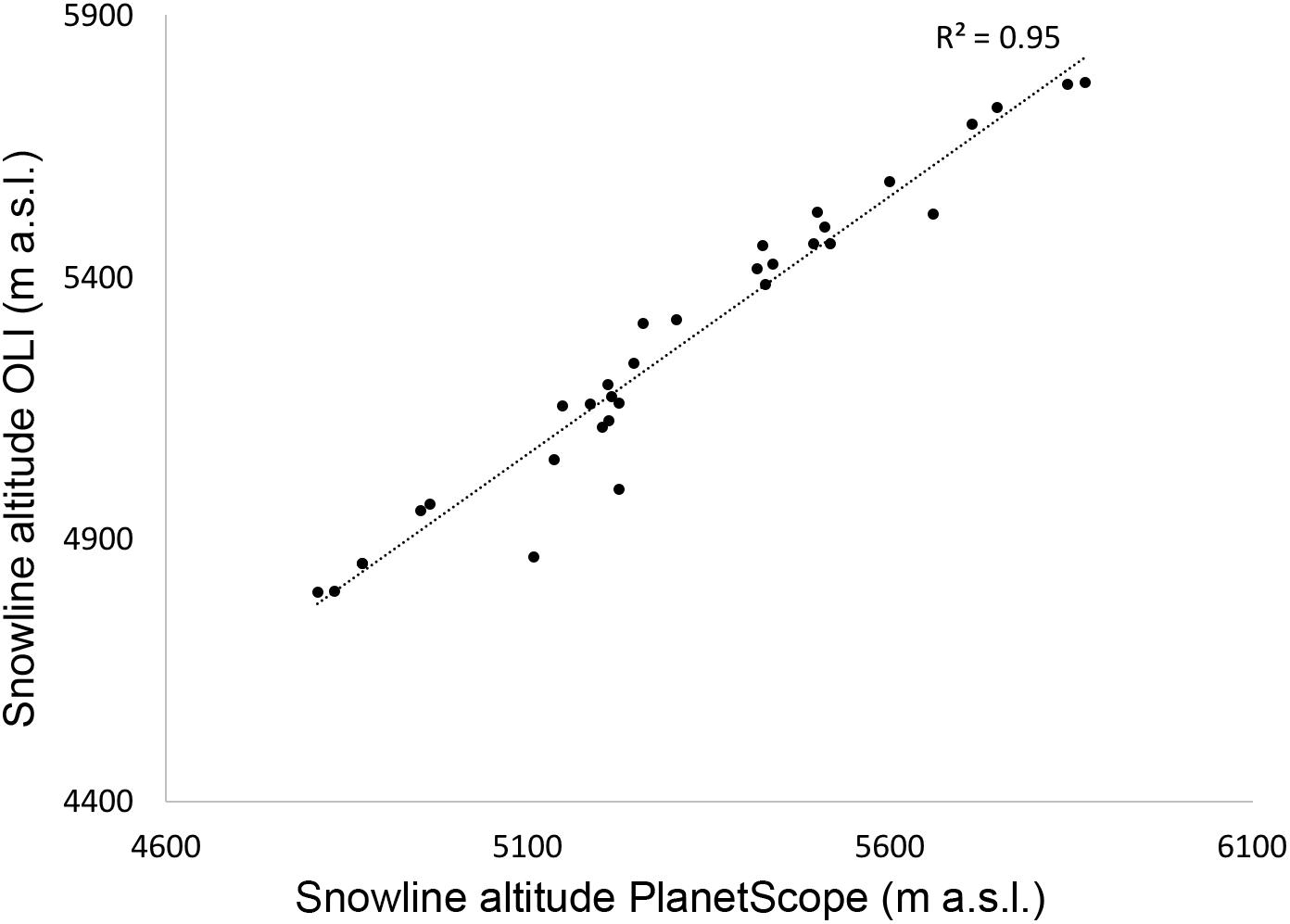
Figure 9. Comparison between semi-automated Landsat OLI SLA with manually derived PlanetScope SLAs in the Trishuli for the October 25, 2016 image.

Discussion

Spatial Patterns in SLA/ELA and Possible Links With Climate

Spatial patterns in SLAs for the month of October in the Hunza (2013) and in the Trishuli (2016) show a variability in SLA for both areas (Figure 10). In the Hunza (Figure 10A), SLAs decrease by 0.5 m vertical per 1 km eastward and increase by 8 m vertical per 1 km northward. The gradient is oriented slightly in the southeast – northwest direction (176.4°), with lower SLA values in the southeast and higher in the northwest. Our results agree with Mukhopadhyay and Khan (2016), who pointed out a strong east-west gradient in precipitation patterns in this area, causing ELA to vary across the Karakoram from about 4,840 to 6,200 m a.s.l. In the Trishuli subset area (Figure 10B), SLAs increase by 11 m vertical per 1 km eastward and 13 m vertical per 1 km change northward, and the trend is northeast (49.6°). SLA values in the Trishuli exhibit a larger spatial gradient in SLA than in the Hunza, as they increase toward the drier Tibetan Plateau, on the northeast side of our study region. In the Trishuli, SLA values ranged from 4,414 m a.s.l. on the south side of the divide to a maximum of 6,581 m a.s.l. the north side of the divide (Tibetan Plateau), with an average of 5,425 m a.s.l. This is in agreement with our estimates of mean ELA values of 5,468 m a.s.l. in this area from the previous study based on manual digitization on ASTER imagery (Racoviteanu et al., 2013), as well as other studies mentioned previously (Benn and Owen, 2005; Kayastha and Harrison, 2008; Ragettli et al., 2015). The high SLA values of up to 6,581 m a.s.l. in the northern part of the Trishuli area may be due to the drier climate compared to the southern slopes, caused by a decrease in moisture content in the northeast from orographic forcing of monsoon air masses over the Himalaya. The strong gradients in SLA values towards the northeast (Tibetan Plateau) indicate that SLA values calculated over the entire Landsat extent may not be representative of the entire region in this area. To test this, we calculated SLAs separately on the northern slopes of the Himalaya (Tibetan Plateau) and southern slopes (Trishuli basin) of the subset area. Using only the SLA pixels on the southern slopes, we obtained an average SLA of 5,222 m a.s.l., which is about 4% lower than the overall estimates over the entire scene including the Tibetan Plateau (5,425 m a.s.l). On the northern side of the divide, more glacier ice is exposed in late season than on the southern side. The larger expanse of exposed glacier ice on the northern slope, and the higher SLAs appear to bias the regional trends when analyzing the entire Landsat scene in this area. When SLA values are calculated using an entire scene which spans distinct climatic regions, regional SLA values are overestimated by ∼200 m, so a basin-by-basin approach would be more appropriate. This observation has important implications for regional ELA estimates intended for mass balance applications, as glacier trends, including ELA trends, do not often follow hydrologic boundaries.

FIGURE 10

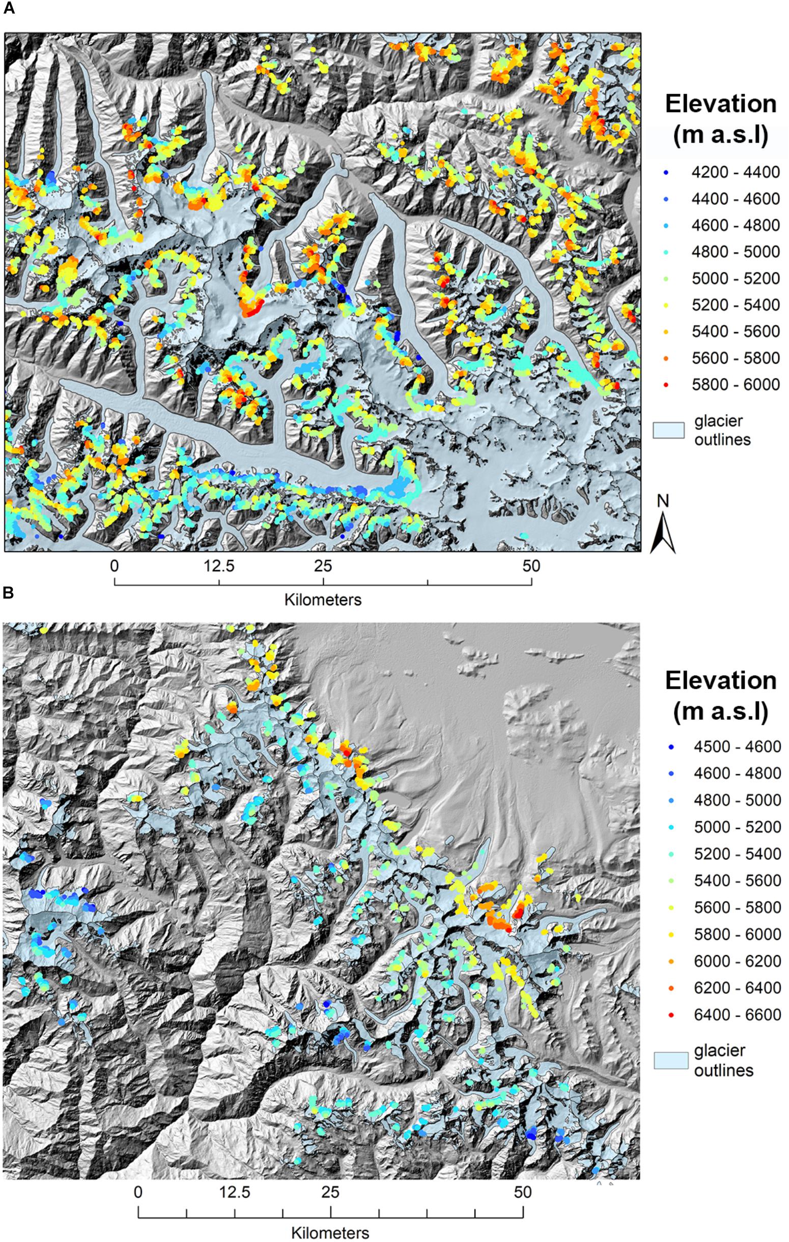
Figure 10. Spatial patterns in snowline altitudes during the month of October represented with a blue (lower SLAs) to red (higher SLAs): (A) Hunza Shimshal valley and (B) Langtang valley in the Trishuli. Each dot represents median elevations of snowlines extracted from the SRTM DEM. Also shown are glacier areas from the Randolph Glacier Inventory (RGI v.6) for reference.

Sensitivity Analysis

While band ratio thresholds are fairly consistent throughout glacierized regions worldwide (e.g., Paul and Andreassen, 2009; Racoviteanu et al., 2009), it is generally advisable that the thresholds be checked in each region. We found that the SLAs were not very sensitive to the threshold used for band ratios to distinguish snow and ice from surrounding terrain. When using thresholds 1.2 and 2, the differences in resulting SLAs ranged from −73 to +26 m, on average −0.2 to −0.04% compared to SLA using the chosen threshold (1.5) (Table 4).

TABLE 4

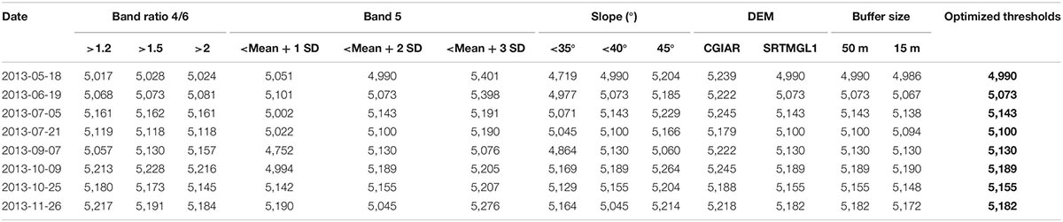
Table 4. Sensitivity of derived snowline altitudes to key parameters used for surface partitioning for the full extent of the Landsat OLI/TIRS imagery using the Hunza monthly series (2013) as test site. No manual corrections were applied for the sensitivity analysis. The “optimized” thresholds used for the final version of the SLAs reported here are based on the sensitivity analysis and adjustments based on visual interpretation. The SLA values resulting from each parameter are reported in m a.s.l.

With respect to OLI band 5 used to distinguish snow from ice on the glacier surface, we tested two thresholds based on statistics extracted from the ROIs: mean + 1 SD and mean + 3 SD (Figure 11). Since the ROIs digitized on glacier tongues and used to extract band ratio statistic were chosen lower in the (darker) ablation areas of glaciers, we estimated that the adequate DN threshold would be above the mean. The sensitivity analysis for Band 5 (Table 4) showed that the SLAs were fairly sensitive to the choice of threshold, with SLA differences ranging from −244 m (underestimate) to +411 m (overestimated). Band 5 DN values calculated over the ice ROIs show seasonal variability (Figure 11). We found that the optimized DN chosen corresponds closely to mean + 1 SD in the spring and late fall months, and to the mean + 2 SD during the summer season (June to October). The average SLA differences were 1–3% lower than those obtained using the optimized threshold. SLA differences were larger in the spring (May) and late fall (November), when snow covered more of the glacier tongues where ROIs were chosen.

FIGURE 11

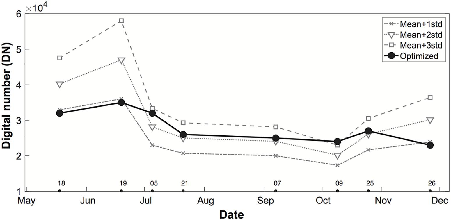
Figure 11. Sensitivity of the calculated SLAs to the choice of DN threshold for Band 5 for the Hunza subset data, based on mean statistics from 20 regions of interest (ROIs) digitized in the ablation area of several glaciers. The DN threshold corresponds to mean + 1 SD for the May–June and December, when the tongues may be covered with snow (brighter), and to mean + 2 SD during July–November when more glacier ice is exposed (darker). The black line shows the “optimized” DN, which was chosen based on the ROI statistics and visual checking using color composites.

Season snowline altitude estimates were sensitive to the topographic slope threshold during the months of May and November (Table 4). For these months, SLA differences ranged from −271 to +214 m, however these were still within our SLA uncertainty estimates for those months (Table 3). During the months at the end of ablation season (October and November), SLA differences ranged from −26 to +63 m. Overall, SLA differences due to the various slope thresholds only amount to −1 to 2% compared to those obtained using the optimized value.

To quantify the sensitivity of the snowlines to the DEM used for the surface partition step (90 m CGIAR vs. 30 m SRTMGL1), we compared SLAs obtained from the uncorrected partitioning for the full extent of the Landsat imagery in the Hunza based on the two DEMs, using the same buffer size (50 m). In this area, the uncorrected SLAs over the full extent of the Landsat scene using the 90 m CGIAR ranged from 5,239 ± 575 m a.s.l. (May) to 5,245 ± 86 m a.s.l (October). Using the 30 m SRTM DEM, resulting SLAs ranged from 4,990 ± 575 m a.s.l. (May) to 5,189 ± 106 m a.s.l. for (October) (Table 4). SLAs obtained using the CGIAR were lower than the values obtained using the SRTMGL1. The differences (CGIAR–SRTMGL1) decreased from the spring and early summer months (May and June) (167 m on average) to the fall months (October–November) (35 m on average) (Table 4). This difference, calculated as percentage of the CGIAR-based SLA, amounts to a maximum of 4.8% in the spring months and a minimum of 0.6% in October. The two sets of SLA estimates were statistically different based on two sample t-tests at 95% confidence interval (p < 0.05), suggesting that the choice of the DEM significantly impacts the snowline estimates. Regardless of the DEM, we consider the SLA results from the spring months to be less reliable due to poorer image quality, more clouds and more snow. When different DEMs were used only in the last step of the analysis (i.e., extracting elevations along the SLAs) from the same version for partition, differences in resulting SLAs were negligible (∼2 m on average). The size of the buffer (50 m vs. 15 m) used to extract the snowlines after surface partition had little impact on the resulting SLAs based on sensitivity tests for the Hunza full extent (Table 4). Differences in SLA calculated using the 50 and 15 m buffers, respectively, ranged from −1 m in October 9 to 10 m on November 26, with an average of +5 m, or +0.1% difference between the two versions (Table 4). We conclude that SLAs are not sensitive to the size of the buffer used to extract the snowlines.

To quantify the impact of manual corrections on the SLAs, we compared the SLA resulting from the uncorrected and corrected surface partition in the Hunza and Trishuli. In the Hunza subset area, SLAs from “uncorrected” surface partition ranged from 5,301 ± 578 m a.s.l. in May 18 to 5,261 ± 254 m a.s.l. on November 26, with a month-to-month variability. After manual corrections, SLAs in the subset area ranged from 4,727 m a.s.l. ± 69 (May) to 5,171 ± 69 m a.s.l. (October), with the biggest difference in the spring month (574 m, or 11%) (Table 3). SLAs resulting from the “corrected” surface partitions were generally lower than the “uncorrected” version (a mean difference of ∼208 m or about 4% of the uncorrected version). The difference in SLA values from uncorrected vs. corrected partition was generally smaller in the summer and fall months (July to October) due to better image quality and less seasonal snow (Figure 7A). For these months, the average difference in median SLAs between these two versions was on average 68 m, about 75% less than the average difference in the spring and winter months (291 m). In the Trishuli subset area, SLAs from “uncorrected” partition in the Trishuli subset ranged from 5,324 ± 27 m a.s.l. in June to a maximum of 5,534 ± 48 m a.s.l. in December (Table 3). After corrections, SLAs in the subset Trishuli ranged from 5,261 m a.s.l. in June to 5,495 m a.s.l. in December, with the biggest difference between the uncorrected and the corrected version in the summer month (June) (63 m difference, or 1.2%). After the corrections, similarly to the Hunza, SLAs in Trishuli were on average lower than before the corrections (a mean difference of 39 m, or 0.7% compared to the uncorrected values) (Figure 7B). Most likely, the lower SLAs after corrections are due to removal of shadows in accumulation area, initially misclassified as ice. To assess the effectiveness of the manual corrections, we used a paired t-test on the pre-corrected and post-corrected versions. The test indicated that SLAs computed after the manual corrections were statistically different than those issued from the uncorrected version at 95% confidence interval (p < 0.05) in both areas, implying that the corrections significantly changed the mean values. Similarly to the Hunza, in the Trishuli subset area, after manual corrections of the surface partition, SLA values were statistically different than the ones obtained from the uncorrected partition (Table 3), based on two-sample t-test at 95% confidence interval, p < 0.05.

Continuity From Landsat 7 ETM+ to Landsat 8 OLI and Impact on Estimated ELA

The temporal trends of ELA may be subject to uncertainties associated with the Landsat sensors used: ETM+ (2000–2012) and OLI (2013–2016), and with respect to the transition from ETM+ to OLI in 2013. In this study, we used Landsat L1T products (pre-collection) and L1TP T1 (collection 1), which are registered, radiometrically calibrated and orthorectified using ground control points GCPs and a DEM (USGS, 2015). These products have stated 50 m global geolocation accuracy, but the actual accuracy was found to be better than the projected. The alignment of the scenes with respect to one another was assessed visually, and further co-registration was not considered necessary. A source of error in the Landsat 7 ETM+ is that scenes acquired after 2003 had the scan line corrector (SLC) turned off due to failure and have data gaps, visible as “stripes” on the images. These were more pronounced toward the edges of the images in our study area, and they were treated as “NoData” in our study. The gaps in the data decrease the total sample size for Landsat 7, when present. The Landsat 8 data used after 2013 has several advantages with respect to ETM+, notably narrower spectral bands, improved calibration and signal-to-noise ratio (SNR), better geometry and 12-bit radiometric resolution compared to 8-bit for Landsat ETM+ (Irons et al., 2012). Landsat OLI data are not saturated, while Landsat ETM+ has pixels that are saturated in bands 1, 2, or 3 (the visible bands), which may appear darker than they really are. In addition, the USGS uses cubic-convolution resampling to smooth the data, not nearest neighbor resampling. As a result, saturated pixels can be mixed with nearby un-saturated ones in this resampling, making it difficult to identify and exclude those from our analysis. Overall, we consider the results from OLI to be more reliable based on these characteristics, with an accuracy of 50 m based on comparison with PlanetScope (section “Uncertainty Estimates”). As no clear ETM+ vs. OLI trend was detected, we did not attempt any inter-calibration, but future studies might consider this issue.

Limitations and Further Work

Delineating the snow/firn-ice boundary using remote sensing in mountainous terrain using optical remote sensing is challenging due to shadows, since snow in shadow appears spectrally similar to clean ice or dirty ice in the ablation area of glaciers. Limitations of the current study include:

• Our method does not allow making the distinction between snowline and firnline, but we acknowledge that under warming conditions, the snowline may retreat beyond the firnline. Applying this method on daily high-resolution imagery may facilitate this distinction.

• Distinguishing snow on land from snow on ice remains a challenge, since snow has the same spectral signature on and off the glacier; here we relied on a glacier mask at each step.

• Band ratio algorithms, while fairly robust, are prone to misclassification errors over frozen lakes and deep/cast shadows over snow and ice (Racoviteanu et al., 2009). Using topographically corrected surface reflectance to reduce variability in illumination instead of top of atmosphere data might mitigate post-classification correction efforts.

• Some snowlines are obscured by shadow and they often do not appear as continuous lines, which may slightly bias our regional estimates especially in areas which span different climatic areas.

• The thresholds used for surface partition rely on a-priory knowledge to some extent. Using a single threshold is challenging in rough terrain due to differences in topographic illumination or image saturation as well as climatic differences across regions. However, in this study, we used a consistent threshold across all images as much as possible.

• Further steps to improve the efficacy of our algorithm include more sophisticated cloud mapping techniques and automated shadow detection using sub-pixel methods (Sirguey et al., 2009).

• Post-classification manual corrections of the surface partition were most needed for spring and winter image(s), with minimal corrections and greater accuracy for images acquired later in the season, which were more contrasted and generally cloud-free. We developed tools to automate the post-classification corrections in areas of shadow over snow in the accumulation areas to reduce the time needed for manual edits.

• SLA/ELA estimates are limited to monthly temporal resolutions due to the revisit time of the Landsat imagery (16 days), but the method can be easily applied to Sentinel-2 data (5 days). With further testing and refinement and perhaps calibration with field measurements of SLA/ELA, this method can be modified for daily satellite data such as PlanetScope to derive sub-monthly SLAs.

Conclusion

Manual digitization of snow and ice on glaciers and subsequent extraction of SLAs is generally a time-consuming process and is difficult to apply over large areas, especially when time series of the snowlines are needed. Here we developed an automated method to separate snow-ice-debris surfaces in two areas of the Himalayas at multi-temporal scales based on Landsat ETM+ and OLI band ratios and topographic criteria. We extracted snowline elevations pixel-by-pixel and estimated ELAs in two areas of HMA: Hunza and Trishuli at monthly time scales (2013 and 2016, respectively) and annual time scales (2000–2016). SLA estimates were significantly sensitive to the manual corrections applied to the snow and ice partition results, and fairly sensitive to the topographic slope, the DEM and the band ratio thresholds, particularly during the spring and winter months due to more snow. Snowlines were less sensitive to the size of the buffer used to extract the snowlines.

Using this method, we obtained a maximum SLA (∼ELA) of 5,171 ± 27 m a.s.l. in October of 2013 for the Hunza and 5,495 ± 27 m a.s.l. for the month of December of 2016 for the Trishuli., after manual corrections. Over the period studied (2000–2016), end-of-the-ablation season annual ELAs fluctuated from 4,917 to 5,336 m a.s.l. for the Hunza, with a 16-year average of 5,177 ± 108 m a.s.l., and 5,395 to 5,565 m a.s.l. for the Trishuli, with an average of 5,444 ± 63 m a.s.l. SLA trends obtained over a smaller subset of the Landsat scenes were representative of the full extent of the image, with an average difference of 100 m. We consider that regional SLA/ELA values obtained using this method are adequate for regional applications such as melt models, when image quality, time of the year, uncertainties due to the DEM used, and band ratio thresholds are considered and assessed. Caution is needed when extracting a “regional” annual ELA value when an image spans various climatic regions, as SLAs may be biased. The time series of snow, ice and debris in two regions provides a valuable training dataset, which may be used in future work to classify images using more sophisticated algorithms such as machine learning classifiers, such as random forests.

Data Availability

The datasets generated for this study are available on request to the corresponding author.

Author Contributions

AR ordered and processed the satellite imagery, developed the python scripts and remote sensing methods to partition the different surfaces and to extract the snowlines, and was also responsible for writing the main body of the manuscript. KR contributed to the development of the algorithm though versioning and feedback, figure generation, and extensive manuscript editing. RA contributed to the theoretical glaciological concepts and manuscript editing. All authors contributed to this work.

Funding

AR, KR, and RA were primarily supported by the Contribution to High Asian Runoff from Ice and Snow (CHARIS) project, funded by the United States Agency for International Development (USAID, Cooperative Agreement No. AID-0AA-A-11-00045). Additional support for AR was from the European Union’s Horizon 2020 Research and Innovation Programme under the Marie Skłodowska-Curie grant agreement No 663830. KR was also supported by the NASA Applied Science Grant 80NSSC18K0427 and the NASA HiMAT project.

Conflict of Interest Statement

The authors declare that the research was conducted in the absence of any commercial or financial relationships that could be construed as a potential conflict of interest.

Acknowledgments

We acknowledge the CHARIS project; the USGS EROS Data Center for providing free access to the Landsat imagery; the Randolph Consortium for providing the glacier outlines; the Planet Labs Inc., for providing free access to the PlanetScope imagery through their API program; and Antoine Rabatel for providing his feedback and suggestions on the snowline mapping.

Footnotes

1. ^ nsidc.org/charis

References

Acharya, A., and Kayastha, R. B. (2019). Mass and energy balance estimation of Yala Glacier (2011–2017), Langtang Valley, Nepal. Water 11:6. doi: 10.3390/w11010006

CrossRef Full Text | Google Scholar

Ageta, Y., and Higuchi, K. (1984). Estimation of mass balance components of a summer-accumulation type glacier in the Nepal Himalaya. Geogr. Ann. Ser. A 66, 249–255. doi: 10.1080/04353676.1984.11880113

CrossRef Full Text | Google Scholar

Andreassen, L. M., Paul, F., Kääb, A., and Hausberg, J. E. (2008). The new Landsat-derived glacier inventory for Jotunheimen, Norway, and deduced glacier changes since the 1930s. Cryosphere Discuss. 2, 299–339. doi: 10.5194/tcd-2-299-2008

CrossRef Full Text | Google Scholar

Armstrong, R. L., Rittger, K., Brodzik, M. J., Racoviteanu, A., Barrett, A. P., Khalsa, S.-J. S., et al. (2019). Runoff from glacier ice and seasonal snow in High Mountain Asia: separating melt water sources in river flow. Reg. Environ. Change 19, 1249–1261. doi: 10.1007/s10113-018-1429-0

CrossRef Full Text | Google Scholar

Azam, M. F., Wagnon, P., Berthier, E., Vincent, C., Fujita, K., and Kargel, J. S. (2018). Review of the status and mass changes of Himalayan-Karakoram glaciers. J. Glaciol. 64, 61–74. doi: 10.1017/jog.2017.86

CrossRef Full Text | Google Scholar

Barandun, M., Huss, M., Usubaliev, R., Azisov, E., Berthier, E., Kääb, A., et al. (2018). Multi-decadal mass balance series of three Kyrgyz glaciers inferred from modelling constrained with repeated snow line observations. Cryosphere 12, 1899–1919. doi: 10.5194/tc-12-1899-2018

CrossRef Full Text | Google Scholar

Benn, D., and Owen, L. A. (2005). Equilibrium-line altitudes of the last glacial maximum for the Himalaya and Tibet: an assessment and evaluation of results. Quat. Int. 138-139, 55–58.

Google Scholar

Benn, D. I., and Owen, L. A. (1998). The role of the Indian summer monsoon and the mid-latitude westerlies in Himalayan glaciation: review and speculative discussion. J. Geol. Soc. 155, 353–363. doi: 10.1144/gsjgs.155.2.0353

CrossRef Full Text | Google Scholar

Benn, D. I., Owen, L. A., Osmaston, H. A., Seltzer, G. O., Porter, S. C., and Mark, B. (2005). Reconstruction of equilibrium-line altitudes for tropical and sub-tropical glaciers. Quat. Int. 138-139, 8–21. doi: 10.1016/j.quaint.2005.02.003

CrossRef Full Text | Google Scholar

Berthier, E., Arnaud, Y., Vincent, C., and Remy, F. (2006). Biases of SRTM in high-mountain areas: implications for the monitoring of glacier volume changes. Geophys. Res. Lett. 33:L08502. doi: 10.01029/02006GL025862

CrossRef Full Text | Google Scholar

Bolch, T., Kulkarni, A., Kääb, A., Huggel, C., Paul, F., Cogley, J. G., et al. (2012). The state and fate of Himalayan Glaciers. Science 336:310. doi: 10.1126/science.1215828

PubMed Abstract | CrossRef Full Text | Google Scholar

Bolch, T., Menounos, B., and Wheate, R. (2010). Landsat-based inventory of glaciers in western Canada, 1985–2005. Remote Sens. Environ. 114, 127–137. doi: 10.1016/j.rse.2009.08.015

CrossRef Full Text | Google Scholar

Bookhagen, B., and Burbank, D. W. (2006). Topography, relief and TRMM-derived rainfall variations along the Himalaya. Geophys. Res. Lett. 33:L08405. doi: 10.1029/2006gl026037

CrossRef Full Text | Google Scholar

Bookhagen, B., and Burbank, D. W. (2010). Toward a complete Himalyan hydrological budget: spatiotemporal distribution of snowmlet ad rainfall and their impact on river discharge. J. Geophys. Res. 115:F03019. doi: 10.1029/2009JF001426

CrossRef Full Text | Google Scholar

Braithwaite, R., and Raper, S. (2009). Estimating equilibrium-line altitude (ELA) from glacier inventory data. Ann. Glaciol. 50, 127–132. doi: 10.3189/172756410790595930

CrossRef Full Text | Google Scholar

Brun, F., Berthier, E., Wagnon, P., Kääb, A., and Treichler, D. (2017). A spatially resolved estimate of High Mountain Asia glacier mass balances from 2000 to 2016. Nat. Geosci. 10:668. doi: 10.1038/ngeo2999

PubMed Abstract | CrossRef Full Text | Google Scholar

Dyurgerov, M. (1996). Substitution of long-term mass balance data by measurements of one summer. Z. Gletscherkunde Glazialgeol. 32, 177–184.

Google Scholar

Dyurgerov, M., Meier, M. F., and Bahr, D. B. (2009). A new index of glacier area change: a tool for glacier monitoring. J. Glaciol. 55, 710–716. doi: 10.3189/002214309789471030

CrossRef Full Text | Google Scholar

Forsythe, N., Fowler, H. J., Li, X.-F., Blenkinsop, S., and Pritchard, D. (2017). Karakoram temperature and glacial melt driven by regional atmospheric circulation variability. Nat. Clim. Change 7, 664–670. doi: 10.1038/nclimate3361

CrossRef Full Text | Google Scholar

Fowler, H. J., and Archer, D. R. (2006). Conflicting signals of climatic change in the Upper Indus Basin. J. Clim. 19, 4276–4293. doi: 10.1175/jcli3860.1

CrossRef Full Text | Google Scholar

Fujita, K., and Nuimura, T. (2011). Spatially heterogeneous wastage of Himalayan glaciers. Proc. Natl. Acad. Sci. U.S.A. 108, 14011–14014. doi: 10.1073/pnas.1106242108

PubMed Abstract | CrossRef Full Text | Google Scholar

Fujita, K., Suzuki, R., Nuimura, T., and Sakai, A. (2008). Performance of ASTER and SRTM DEMs, and their potential for assessing glacial lakes in the Lunana region, Bhutan Himalaya. J. Glaciol. 54, 220–228. doi: 10.3189/002214308784886162

CrossRef Full Text | Google Scholar

Gardelle, J., Berthier, E., Arnaud, Y., and Kaab, A. (2013). Region-wide glacier mass balances over the Pamir-Karakoram-Himalaya during 1999-2011 (vol 7, pg 1263, 2013). Cryosphere 7, 1885–1886. doi: 10.5194/tc-7-1885-2013

CrossRef Full Text | Google Scholar

Garg, P. K., Shukla, A., and Jasrotia, A. S. (2017). Influence of topography on glacier changes in the central Himalaya, India. Glob. Planet. Change 155, 196–212. doi: 10.1016/j.gloplacha.2017.07.007

CrossRef Full Text | Google Scholar

Granshaw, F. D., and Fountain, A. (2017). Glacier change (1958–1998) in the North Cascades National Park Complex, Washington, USA. J. Glaciol. 52, 251–256. doi: 10.3189/172756506781828782

CrossRef Full Text | Google Scholar

Guo, Z., Wang, N., Kehrwald, N. M., Mao, R., Wu, H., Wu, Y., et al. (2014). Temporal and spatial changes in Western Himalayan firn line altitudes from 1998 to 2009. Glob. Planet. Change 118, 97–105. doi: 10.1016/j.gloplacha.2014.03.012

CrossRef Full Text | Google Scholar

Hewitt, K. (2005). The Karakoram anomaly- Glacier expansion and the -elevation effect,- Karakoram Himalaya. Mt. Res. Dev. 25, 332–340. doi: 10.1659/0276-4741(2005)025

CrossRef Full Text | Google Scholar

Hewitt, K. (2011). Glacier Change, Concentration, and Elevation Effects in the Karakoram Himalaya, Upper Indus Basin. Mt. Res. Dev. 31, 188–200. doi: 10.1659/MRD-JOURNAL-D-11-00020.1

CrossRef Full Text | Google Scholar

Huss, M., and Hock, R. (2015). A new model for global glacier change and sea-level rise. Front. Earth Sci. 3:54. doi: 10.3389/feart.2015.00054

CrossRef Full Text | Google Scholar

Huss, M., Sold, L., Hoelzle, M., Stokvis, M., Salzmann, N., Farinotti, D., et al. (2013). Towards remote monitoring of sub-seasonal glacier mass balance. Ann. Glaciol. 63, 75–83. doi: 10.3189/2013aog63a427

CrossRef Full Text | Google Scholar

Irons, J. R., Dwyer, J. L., and Barsi, J. A. (2012). The next landsat satellite: the landsat data continuity mission. Remote Sens. Environ. 122, 11–21. doi: 10.1016/j.rse.2011.08.026

CrossRef Full Text | Google Scholar

Jarvis, A., Reuter, H. I., Nelson, A., and Guevara, E. (2008). Hole-filled Seamless SRTM Data V4, International Centre for Tropical Agriculture (CIAT) [Online]. Available at: http://srtm.csi.cgiar.org (accessed July 17, 2018).

Google Scholar

Kääb, A., Berthier, E., Nuth, C., Gardelle, J., and Arnaud, Y. (2012). Contrasting patterns of early twenty-first-century glacier mass change in the Himalayas. Nature 488, 495–498. doi: 10.1038/nature11324

PubMed Abstract | CrossRef Full Text | Google Scholar

Kaser, G., and Osmaston, H. A. (2002). Tropical Glaciers. Oxford: Cambridge University Press.

Google Scholar

Kayastha, R. B., and Harrison, S. P. (2008). Changes of the equilibrium-line altitude since the Little Ice Age in the Nepalese Himalaya. Ann. Glaciol. 48, 93–99. doi: 10.3189/172756408784700581

CrossRef Full Text | Google Scholar

Khalsa, S. J. S., Dyurgerov, M. B., Khromova, T., Raup, B. H., and Barry, R. G. (2004). Space-based mapping of glacier changes using ASTER and GIS tools. IEEE Trans. Geosci. Remote Sens. 42, 2177–2183. doi: 10.1109/tgrs.2004.834636

CrossRef Full Text | Google Scholar

Khan, A., Naz, B. S., and Bowling, L. C. (2015). Separating snow, clean and debris covered ice in the Upper Indus Basin, Hindukush-Karakoram-Himalayas, using Landsat images between 1998 and 2002. J. Hydrol. 521, 46–64. doi: 10.1016/j.jhydrol.2014.11.048

CrossRef Full Text | Google Scholar

Kienholz, C., Hock, R., Truffer, M., Bieniek, P., and Lader, R. (2017). Mass balance evolution of Black Rapids Glacier, Alaska, 1980–2100, and its implications for surge recurrence. Front. Earth Sci. 5, 56. doi: 10.3389/feart.2017.00056

CrossRef Full Text | Google Scholar

King, O., Quincey, D. J., Carrivick, J. L., and Rowan, A. V. (2017). Spatial variability in mass loss of glaciers in the Everest region, central Himalayas, between 2000 and 2015. Cryosphere 11, 407–426. doi: 10.5194/tc-11-407-2017

CrossRef Full Text | Google Scholar

Klein, A. G., and Isacks, B. L. (1999). Spectral mixture analysis of Landsat thematic mapper images applied to the detection of the transient snowline on tropical Andean glaciers. Glob. Planet. Change 22, 139–154. doi: 10.1016/S0921-8181(99)00032-6

CrossRef Full Text | Google Scholar

Kulkarni, A. V. (1992). Mass balance of Himalayan Glaciers using AAR and ELA methods. J. Glaciol. 38, 101–104. doi: 10.1017/s0022143000009631

PubMed Abstract | CrossRef Full Text | Google Scholar

Kulkarni, A. V., Rathore, B. P., and Alex, S. (2004). Monitoring of glacial mass balance in the Baspa basin using accumulation area ratio method. Curr. Sci. 86, 185–190.

Google Scholar

Leonard, K. C., and Fountain, A. G. (2017). Map-based methods for estimating glacier equilibrium-line altitudes. J. Glaciol. 49, 329–336. doi: 10.3189/172756503781830665

CrossRef Full Text | Google Scholar

Llibutry, L. (1998). “Glaciers of the dry Andes,” in Satellite Image Atlas of Glaciers of the World: South America, eds R. S. J. Williams and J. G. Ferrigno (Reston, VA: United States Geological Survey).

Google Scholar

Meier, M. (1962). Proposed definitions for glacier mass budget terms. J. Glaciol. 4, 252–261.

Google Scholar

Meier, M. F., and Post, A. S. (1962). “Recent variations in mass net budgets of glaciers in western North America,” in Proceedings of Symposium of Obergurgl, 1962, (Obergurgl: IASH-AISH Publication), 63–67.

Google Scholar

Minora, U., Bocchiola, D., D’Agata, C., Maragno, D., Mayer, C., Lambrecht, A., et al. (2016). Glacier area stability in the Central Karakoram National Park (Pakistan) in 2001–2010: the “Karakoram Anomaly” in the spotlight. Prog. Phys. Geogr. 40, 629–660. doi: 10.1177/0309133316643926

CrossRef Full Text | Google Scholar

Mukhopadhyay, B., and Khan, A. (2016). Altitudinal variations of temperature, equilibrium line altitude, and accumulation-area ratio in Upper Indus Basin. Hydrol. Res. 48, 214–230. doi: 10.2166/nh.2016.144

CrossRef Full Text | Google Scholar

Mukul, M., Srivastava, V., Jade, S., and Mukul, M. (2017). Uncertainties in the shuttle radar topography mission (SRTM) heights: insights from the Indian Himalaya and Peninsula. Sci. Rep. 7:41672. doi: 10.1038/srep41672

PubMed Abstract | CrossRef Full Text | Google Scholar

NASA-JPL (2013). NASA Shuttle Radar Topography Mission Global 1 Arc Second [Data set]. Pasadena, CA: NASA-JPL.

Google Scholar

Ohmura, A., and Boettcher, M. (2018). Climate on the equilibrium line altitudes of glaciers: theoretical background behind Ahlmann’s P/T diagram. J. Glaciol. 64, 489–505. doi: 10.1017/jog.2018.41

CrossRef Full Text | Google Scholar

Osmaston, H. A. (2005). Estimates of glacier equilibrium line altitudes by the area×altitude, the area×altitude balance ratio and the area×altitude balance index methods and their validation. Quat. Int. 138-139, 22–31. doi: 10.1016/j.quaint.2005.02.004

CrossRef Full Text | Google Scholar

Paterson, W. S. B. (1994). The Physics of Glaciers, 3rd Edn. Oxford: Pergamon.

Google Scholar

Paul, F., and Andreassen, L. M. (2009). A new glacier inventory for the Svartisen region, Norway, from Landsat ETM+ data: challenges and change assessment. J. Glaciol. 55, 607–618. doi: 10.3189/002214309789471003

CrossRef Full Text | Google Scholar

Paul, F., Barrand, N., Berthier, E., Bolch, T., Casey, K., Frey, H., et al. (2013). On the accuracy of glacier outlines derived from remote sensing data. Ann. Glaciol. 54, 171–182. doi: 10.3189/2013AoG63A296

CrossRef Full Text | Google Scholar

Paul, F., Kääb, A., Maisch, M., Kellenberger, T., and Haeberli, W. (2002). The new remote-sensing-derived Swiss glacier inventory: I. Methods. Ann. Glaciol. 34, 355–361. doi: 10.3189/172756402781817941

CrossRef Full Text | Google Scholar

Pellicciotti, F., Stephan, C., Miles, E., Herreid, S., Immerzeel, W. W., and Bolch, T. (2015). Mass-balance changes of the debris covered glaciers in the Langtang Himal, Nepal, from 1974 to 1999. J. Glaciol. 61, 373–386. doi: 10.3189/2015jog13j237

CrossRef Full Text | Google Scholar

Pfeffer, W. T., Arendt, A. A., Bliss, A., Bolch, T., Cogley, J. G., Gardner, A. S., et al. (2014). The Randolph Glacier inventory: a globally complete inventory of glaciers. J. Glaciol. 60, 537–552. doi: 10.3189/2014JoG13J176

CrossRef Full Text | Google Scholar

Planet_Team (2017). Planet Application Program Interface. Space for Life on Earth [Online]. Available at: https://api.planet.com (accessed August 25, 2019).

Google Scholar

Rabatel, A., Bermejo, A., Loarte, E., Soruco, A., Gomez, J., Leonardini, G., et al. (2012). Can the snowline be used as an indicator of the equilibrium line and mass balance for glaciers in the outer tropics? J. Glaciol. 58, 1027–1036. doi: 10.3189/2012JoG3112J3027

CrossRef Full Text | Google Scholar

Rabatel, A., Dedieu, J.-P., Thibert, E., Letreguilly, A., and Vincent, C. (2008). Twenty-five years of equilibrium-line altitude and mass balance reconstruction on the Glacier Blanc, French Alps (1981-2005), using remote-sensing method and meteorological data. J. Glaciol. 54, 307–314. doi: 10.3189/002214308784886063

CrossRef Full Text | Google Scholar

Rabatel, A., Dedieu, J. P., and Vincent, C. (2005). Using remote-sensing data to determine equilibrium-line altitude and mass-balance time series: validation on three French glaciers, 1994-2002. J. Glaciol. 51, 539–546. doi: 10.3189/172756505781829106

CrossRef Full Text | Google Scholar

Rabatel, A., Sirguey, P., Drolon, V., Maisongrande, P., Arnaud, Y., Berthier, E., et al. (2017). Annual and seasonal glacier wide surface mass balance quantified from changes in glacier surface state: a review on existing methods using optical satellite imagery. Remote Sens. 9:507. doi: 10.3390/rs9050507

CrossRef Full Text | Google Scholar

Rabus, B., Eineder, M., Roth, A., and Bamler, R. (2003). The shuttle radar topography mission–a new class of digital elevation models acquired by spaceborne radar. ISPRS J. Photogram Rem. Sens. 57, 241–262. doi: 10.1016/s0924-2716(02)00124-7

CrossRef Full Text | Google Scholar

Racoviteanu, A., Paul, F., Raup, B., Khalsa, S. J. S., and Armstrong, R. (2009). Challenges and recommendations in mapping of glacier prameters from space: results of the 2008 Global Land Ice Measurements frpom Space (GLIMS) workshop, Boulder, Colorado, USA. Ann. Glaciol. 50, 53–69. doi: 10.3189/172756410790595804

CrossRef Full Text | Google Scholar

Racoviteanu, A. E., Armstrong, R., and Williams Mark, W. (2013). Evaluation of an ice ablation model to estimate the contribution of melting glacier ice to annual discharge in the Nepal Himalaya. Water Resourc. Res. 49, 5117–5133. doi: 10.1002/wrcr.20370

CrossRef Full Text | Google Scholar

Racoviteanu, A. E., Arnaud, Y., Williams, M. W., and Manley, W. F. (2015). Spatial patterns in glacier characteristics and area changes from 1962 to 2006 in the Kanchenjunga,ÄìSikkim area, eastern Himalaya. Cryosphere 9, 505–523. doi: 10.5194/tc-9-505-2015

CrossRef Full Text | Google Scholar

Racoviteanu, A. E., and Williams, M. W. (2012). Decision tree and texture analysis for mapping debris covered glaciers: a case study from Kangchenjunga, eastern Himalaya. Remote Sens. Spec. Issue 4, 3078–3109. doi: 10.3390/rs4103078

CrossRef Full Text | Google Scholar

Ragettli, S., Pellicciotti, F., Immerzeel, W. W., Miles, E. S., Petersen, L., Heynen, M., et al. (2015). Unraveling the hydrology of a Himalayan catchment through integration of high resolution in situ data and remote sensing with an advanced simulation model. Adv. Water Resourc. 78, 94–111. doi: 10.1016/j.advwatres.2015.01.013

CrossRef Full Text | Google Scholar

Rashid, I., Abdullah, T., Glasser, N. F., Naz, H., and Romshoo, S. A. (2018). Surge of Hispar Glacier, Pakistan, between 2013 and 2017 detected from remote sensing observations. Geomorphology 303, 410–416. doi: 10.1016/j.geomorph.2017.12.018

CrossRef Full Text | Google Scholar

Raup, B., Racoviteanu, A., Singh Khalsa, S. J., Helm, C., Armstrong, R., and Arnaud, Y. (2007). The GLIMS geospatial glacier database: a new tool for studying glacier change. Glob. Planet. Change 56, 101–110. doi: 10.1016/j.gloplacha.2006.07.018

CrossRef Full Text | Google Scholar

Reuter, H. I., Nelson, A., and Jarvis, A. (2007). An evaluation of void filling interpolation methods for SRTM data. Int. J. Geogr. Inform. Sci. 21, 983–1008. doi: 10.1080/13658810601169899

CrossRef Full Text | Google Scholar

Scherler, D., Bookhagen, B., and Strecker, M. R. (2011). Spatially variable response of Himalayan glaciers to climate change affected by debris cover. Nat. Geosci. 4, 156–159. doi: 10.1038/ngeo1068

CrossRef Full Text | Google Scholar

Shrestha, M. L. (2000). Interannual variation of summer monsoon rainfall over Nepal and its relation to the Souther Oscillation index. Meteor. Atmos. Phys. 75, 21–28. doi: 10.1007/s007030070012

CrossRef Full Text | Google Scholar

Sirguey, P., Mathieu, R., and Arnaud, Y. (2009). Subpixel monitoring of the seasonal snow cover with MODIS at 250¬†m spatial resolution in the Southern Alps of New Zealand: methodology and accuracy assessment. Remote Sens. Environ. 113, 160–181. doi: 10.1016/j.rse.2008.09.008

CrossRef Full Text | Google Scholar

Thakur, P. K., Aggarwal, S. P., Arun, G., Sood, S., Senthil Kumar, A., Mani, S., et al. (2017). Estimation of snow cover area, snow physical properties and glacier classification in parts of Western Himalayas using C-Band SAR data. J. Indian Soc. Remote Sens. 45, 525–539. doi: 10.1007/s12524-016-0609-y

CrossRef Full Text | Google Scholar

Thayyen, R. J., and Gergan, J. T. (2010). Role of glaciers in watershed hydrology: a preliminary study of a “Himalayan catchment”. Cryosphere 4, 115–128. doi: 10.5194/tc-4-115-2010

CrossRef Full Text | Google Scholar

USGS (2015). Landsat Processing Details [Online]. Reston, VA: USGS.

Google Scholar

USGS (2016). Landsat8 (L8) Data Users Handbook. LSDS-1574 Version 2.0. Reston, VA: USGS.

Google Scholar

Wagnon, P., Kumar, R., Arnaud, Y., Linda, A., Sharma, P., Vincent, C., et al. (2007). Four years of mass balance on Chhota Shigri Glacier, Himachal Pradesh, India, a new benchmark glacier in the western Himalaya. J. Glaciol. 53, 603–611. doi: 10.3189/002214307784409306

CrossRef Full Text | Google Scholar

Wagnon, P., Vincent, C., Arnaud, Y., Berthier, E., Vuillermoz, E., Gruber, S., et al. (2013). Seasonal and annual mass balances of Mera and Pokalde glaciers (Nepal Himalaya) since 2007. Cryosphere 7, 1769–1786. doi: 10.5194/tc-7-1769-2013

CrossRef Full Text | Google Scholar

Wu, Y., He, J., Guo, Z., and Chen, A. (2014). Limitations in identifying the equilibrium-line altitude from the optical remote-sensing derived snowline in the Tien Shan, China. J. Glaciol. 60, 1093–1100. doi: 10.3189/2014jog13j221

CrossRef Full Text | Google Scholar

Yanai, M., Li, C., and Song, Z. (1992). Seasonal heating of the Tibetan plateau and its effect on the evolution of the Asian summer monsoon. J. Meteorol. Soc. Jpn. 70, 319–351. doi: 10.2151/jmsj1965.70.1b_319

CrossRef Full Text | Google Scholar

Zhang, Q., and Kang, S. (2017). Glacier snowline altitude variations in the Pamirs, Tajikistan, 1998-2013: insights from remote sensing images. Remote Sens. Lett. 8, 1220–1229. doi: 10.1080/2150704X.2017.1375611

CrossRef Full Text | Google Scholar

Zhao, L., Ding, R., and Moore, J. C. (2016). The High Mountain Asia glacier contribution to sea-level rise from 2000 to 2050. Ann. Glaciol. 57, 223–231. doi: 10.3189/2016AoG71A049

CrossRef Full Text | Google Scholar

Zhu, X., and Helmer, E. H. (2018). An automatic method for screening clouds and cloud shadows in optical satellite image time series in cloudy regions. Remote Sens. Environ. 214, 135–153. doi: 10.1016/j.rse.2018.05.024

CrossRef Full Text | Google Scholar

Zhu, Z., Wang, S., and Woodcock, C. E. (2015). Improvement and expansion of the Fmask algorithm: cloud, cloud shadow, and snow detection for Landsats 4–7, 8, and Sentinel 2 images. Remote Sens. Environ. 159, 269–277. doi: 10.1016/j.rse.2014.12.014

CrossRef Full Text | Google Scholar