A Joint Landsat- and MODIS-Based Reanalysis Approach for Midlatitude Montane Seasonal Snow Characterization

Introduction

Midlatitude montane seasonal snowpacks are a vital part of the global water and energy budget and the resulting snowmelt-driven runoff provides fresh water to a significant fraction of the global population (Barnett et al., 2005; Mankin et al., 2015). However, the lack of in situ data networks in key mountain ranges, i.e., in the Western U.S. where sampling is perhaps densest but still unrepresentative of all elevation ranges (Serreze et al., 1999) to High-Mountain Asia (HMA) where it is essentially non-existent (Rohrer et al., 2013), makes answering basic science questions about the spatio-temporal distribution of snow water mass and how it is changing difficult (Dozier et al., 2016). This necessarily requires that estimates of snow distribution rely on remote sensing data and/or models (i.e., global or regional climate models or offline land surface snow and hydrology models).

While monitoring of snow covered area (SCA) has been measured from space over much of the modern remote sensing era, estimating snow water equivalent (SWE) with spaceborne observations remains elusive (Lettenmaier et al., 2015). This is in part because there is currently no dedicated research or operational satellite specifically designed for retrieving SWE. Large-scale SWE retrieval algorithms have primarily been developed based on active (Ulaby and Stiles, 1980; Tsang et al., 2007) and passive (Chang et al., 1987; Kwon et al., 2017) microwave sensors. However, accurate and generally applicable SWE retrieval algorithms based on these measurements are complicated by many factors including (Li et al., 2017): coarse-scale measurements (in the case of passive microwave sensors) that do not capture sub-grid variations, decreasing sensitivity with respect to deep SWE, and a lack of sensitivity altogether to SWE in forest-covered or wet snow conditions. All of these factors lead to significant retrieval errors, especially in mountainous terrain (Tedesco et al., 2010; Frei et al., 2012).

Physically based modeling in mountain regions has its own set of difficulties with respect to SWE estimation. In the case of coupled land-atmosphere models, significant progress has been made in estimating SWE using regional climate models (e.g., Wrzesien et al., 2018 and references therein), however, snowfall precipitation in complex terrain is highly sensitive to the parameterizations that are used (e.g., Rhoades et al., 2018), which can lead to significant biases in SWE and its distribution. Coarse-gridded general circulation models often significantly smooth topography, requiring the need for downscaling procedures to resolve snow processes (e.g., Pierce et al., 2014). In the case of offline land surface snow modeling, which can be applied at high-enough resolution to resolve topography, biases in precipitation from in situ or other meteorological datasets (Adam and Lettenmaier, 2003) can lead to first-order errors in snow accumulation, while uncertainties in other meteorological fields (e.g., air temperature, radiation), combined with the complexity of the terrain, can lead to significant snowmelt errors (Baldo and Margulis, 2017).

One approach to address these issues is to use ensemble-based data assimilation (DA) methods for SWE estimation. DA methods are attractive because they can naturally incorporate remote sensing observations in ways that take advantage of their spatially distributed nature, while accounting for measurement errors and filling gaps in between measurements that leverage physically based model information. Examples of remote sensing-based DA approaches to snow estimation generally include those that incorporate passive microwave-based data (e.g., Durand and Margulis, 2007; Durand et al., 2009; De Lannoy et al., 2010; Li et al., 2017) and those that use visible/near-infrared based SCA data (e.g., Andreadis and Lettenmaier, 2006; Clark et al., 2006; Su et al., 2008; Arsenault et al., 2013; Girotto et al., 2014a, b; Margulis et al., 2015, 2016a) or combinations thereof (e.g., De Lannoy et al., 2012; Liu et al., 2013; Kumar et al., 2015a). From this body of work, several overarching conclusions have emerged: (1) Methods that rely solely on passive microwave-based data tend to suffer from biases in the retrieved SWE that is assimilated and/or cannot provide SWE at the scales of variation desired due to the coarse-scale of the measurements; (2) Filtering (sequential) methods that assimilate SCA show limited improvement over model-based estimates as they are reliant on the instantaneous SCA-SWE relationship, which is generally weak. Recent applications that assimilate fractional SCA (fSCA), but using a retrospective “smoother” framework (e.g., Girotto et al., 2014a; Margulis et al., 2016a; Cortes and Margulis, 2017) have been shown to perform well by instead leveraging the fact that SWE and the set of SCA data over the course of the melt season have a much higher correlation. In essence, these methods constrain the SWE estimates such that they match the depletion record in the fSCA time series.

In this methodological paper we generalize a previous fSCA DA approach for global-scale applications over midlatitude mountain regions. In particular we are motivated to build a framework capable of deriving snow reanalysis estimates over domains like HMA where in situ meteorological and snow data is extremely limited, thereby limiting knowledge of seasonal snow processes. As such we focus on developing a method that jointly uses Landsat- and MODIS-derived fSCA in an effort to maximize the number of cloud-free images and allow for deriving snow estimates at relatively high resolution (∼500 m). The method is further developed to account for MODIS viewing-angle impacts on fSCA estimates – a factor that is often neglected.

Study Sites

The primary objective of the method presented herein is to provide snow estimates in remote midlatitude montane areas where in situ information is generally limited to non-existent (e.g., HMA). The new method is applied at a site in the Sierra Nevada range of California, where a unique Lidar-derived dataset is used for verification, and is then applied over select sub-domains across HMA to illustrate the technique over domains without verification data. The HMA sample results are the first step in the development of a large-scale HMA reanalysis that is the subject of ongoing work.

Tuolumne Watershed in Sierra Nevada (CA, United States)

The Tuolumne River watershed (Figure 1A) drains ∼1100 km² from the western slopes of the Sierra Nevada in California (central coordinates: 38°N, 119.5°W). The basin is a high-elevation, snow-dominated basin with complex terrain and an elevation range between ∼1600 m to above 3500 m and provides water supply for downstream use from snowmelt-driven runoff. The terrain has aspect values mostly distributed between directions facing NW and SE. Forest cover exists at lower elevations (mostly below ∼2700 m) with fractional forest coverage ranging up to 50%. The climatology of Tuolumne is characterized by a strong seasonal precipitation pattern, with the majority of precipitation falling in the winter (December–March) as a result of frontal and atmospheric river systems that tend to result in ∼11 storms per winter season (on average), often with a few storms contributing to the bulk of the snowpack (Huning and Margulis, 2017). The choice of Tuolumne is made primarily because of the existence of the Airborne Snow Observatory (ASO) data [see Section Verification Data: Airborne Snow Observatory (ASO) Data], which provides a unique set of spatially distributed SWE estimates for evaluation of the method.

FIGURE 1

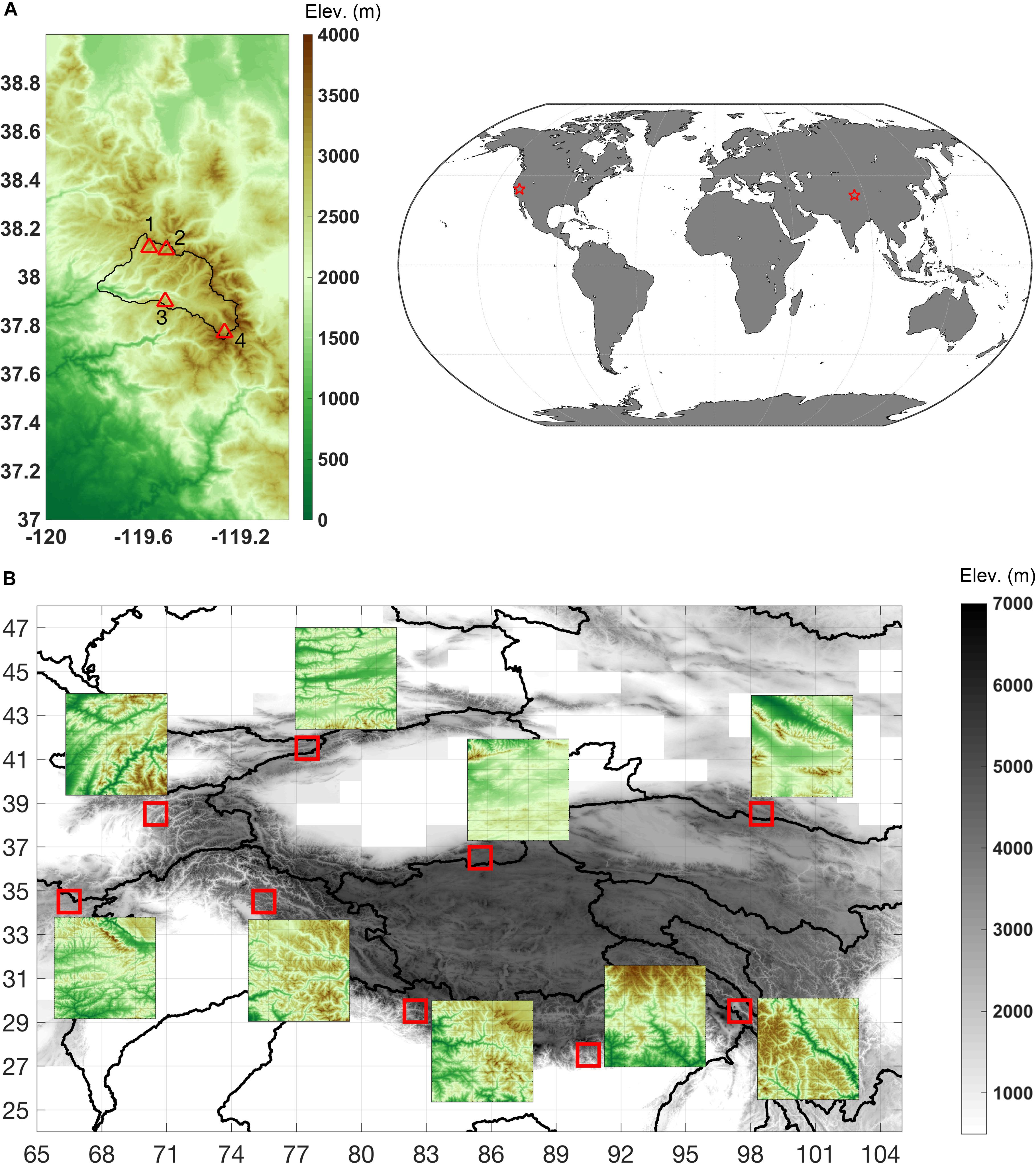
Figure 1. Site maps showing the DEMs (elevations in meters) for (A) the verification site in Tuolumne River watershed in California and (B) the sample tiles across High-Mountain Asia (HMA). The Tuolumne watershed boundary is shown with the black line in panel (A) along with four sample locations used to illustrate verification in Figure 7. Sample tiles over HMA are outlined in red with the color insets showing the respective DEMs in more detail. Inset DEMs do not use the same colorbar range across all tiles, but instead a localized range for each tile to emphasize the spatial patterns that are seen in subsequent figures. The tiles examined are labeled with their lower left corner and consist of: (34°N, 66°E), (4°N, 77°E), (34°N, 75°E), (38°N, 70°E), (29°N, 82°E), (36°N, 85°E), (27°N, 90°E), (29°N, 97°E), (38°N, 98°E).

Test Sub-Domains in High Mountain Asia

After verifying the method over Tuolumne we provide some sample results from sub-domains in HMA. A set of nine 1^° × 1^° tiles are examined in Liu and Margulis (unpublished) to derive a MERRA-2 precipitation uncertainty parameterization for use in generating the forthcoming HMA snow reanalysis dataset. For consistency, we use the same tiles (Figure 1B) herein for illustration of the type of data that will ultimately be generated for the whole HMA domain. The tiles (labeled with their lower left corner) were chosen to sample a range of climatological and physiographic variability across HMA. Four tiles are located in the western part of the domain covering portions of the Hindu Kush, Tien Shan, Pamir, and Karakorum ranges, three tiles are located in the southern part of the domain covering portions of the Himalaya and Hengduan ranges, and the remaining two tiles cover the north central and eastern parts of the domain covering portions of the Kunlun and Qilian ranges. More details on the physiographic and climatological characteristics of the tiles are given in Liu and Margulis (unpublished).

Methods and Data

Bayesian Snow Reanalysis Framework

The method developed and demonstrated herein builds on our previous work (Margulis et al., 2015, 2016a) using a Bayesian snow reanalysis (data assimilation) framework. The “reanalysis” term is used to convey a framework that aims to provide physically based space-time continuous estimates of snow states and fluxes using a snow model that is constrained by remotely sensed snow measurements (in this case fSCA). The methodology is first presented generally, with the specific datasets used as inputs and constraints described in more detail in subsequent sections. The methods and framework are designed with the overarching goal of being globally applicable in any relevant mountainous region.

The specific method presented in this paper is the Particle Batch Smoother (PBS; Margulis et al., 2015). A “smoother” identifies the fact that the fSCA data is assimilated in a single batch (i.e., all images at once) over the full water year (WY) rather than sequentially, as done in a filtering scheme. The primary reason for this choice is that fSCA has limited instantaneous information on SWE, but the depletion (i.e., time series) of fSCA over the melt season, combined with information on energy fluxes that drive snowmelt (via the snow model) is strongly correlated with the evolving SWE time series. Hence it is the batch smoother approach that is primarily responsible for transforming fSCA information into SWE. Such approaches cannot be applied in real-time, but rather provide retrospective estimates once the remotely sensed fSCA time series is available. This is not necessarily a drawback when the goal is to develop historical datasets for improving insight into space-time dynamics of snow processes. The modular framework consists of two main components, highlighted as red and blue boxes in the schematic shown in Figure 2. The first component (red boxes) involves a spatially distributed ensemble-based land surface model-snow depletion curve (LSM-SDC) that is applied to generate so-called prior estimates of snow states and fluxes at each grid cell. The LSM-SDC used herein is the same setup in our previous work with the SSiB-SAST LSM (Sun and Xue, 2001; Xue et al., 2003) coupled to the Liston (2004) SDC, but other models could be used within the framework. The LSM serves to take model inputs (i.e., meteorological time series and static model parameters) and transform them to grid-averaged snow accumulation and surface energy balance fluxes that drive snowmelt. The SDC assumes a lognormal sub-grid distribution for SWE and evolves the grid-averaged SWE and fSCA based on the snow accumulation, melt, and the sub-grid SWE coefficient of variation parameter (β).

FIGURE 2

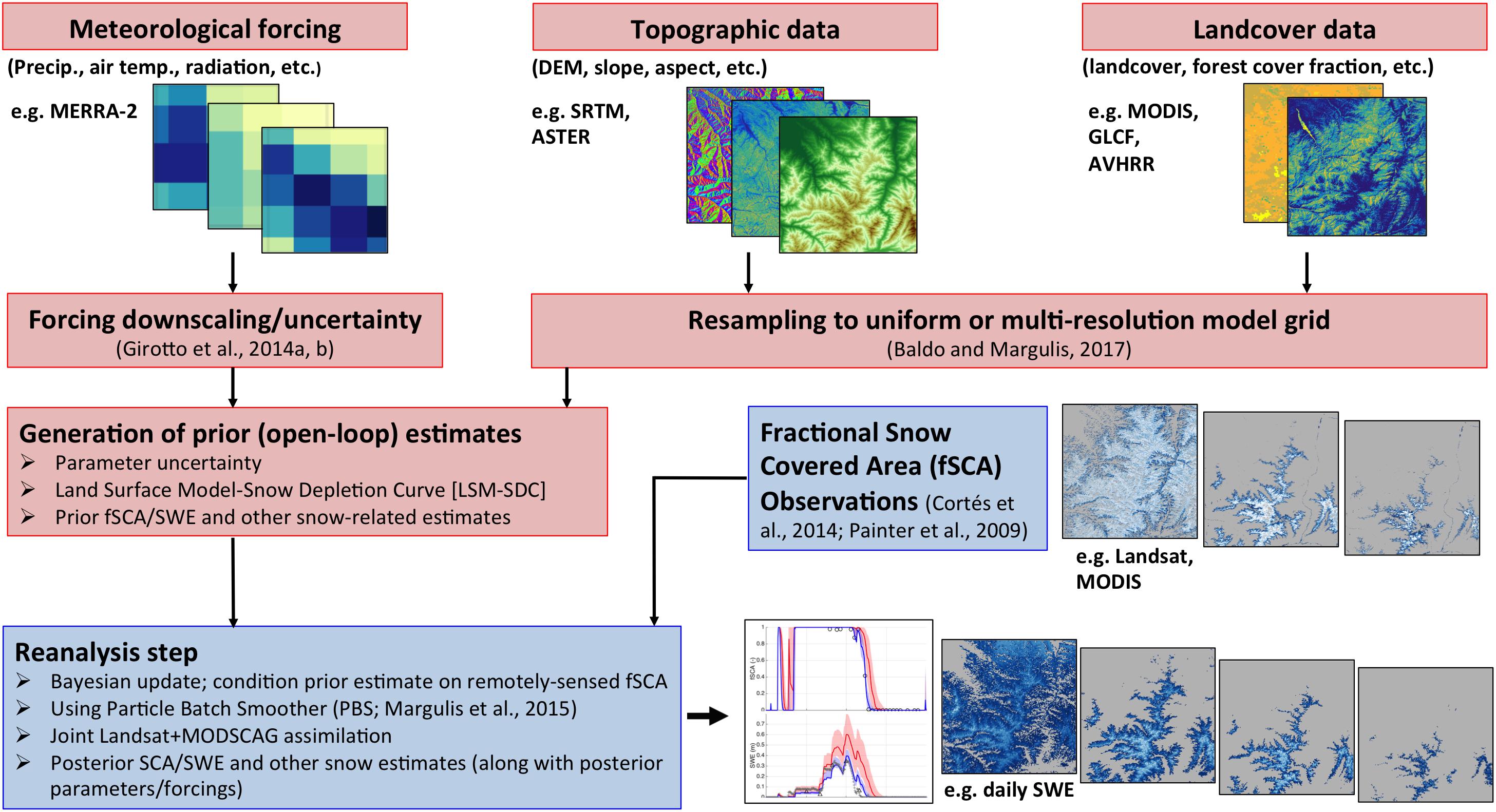
Figure 2. Schematic representation of the Bayesian snow reanalysis framework that consists of an ensemble-based prior modeling system (red boxes) and a posterior update component for assimilating remotely sensed fractional snow covered area (SCA) data from Landsat and MODIS (blue boxes).

Uncertainties in model inputs are a key driver of uncertainty in snow states/fluxes in mountainous environments. The input uncertainties are postulated and explicitly propagated through the modeling framework using an ensemble (Monte-Carlo) approach. Precipitation, which is typically the most important control on SWE accumulation and most uncertain input variable in mountain environments, is treated as follows:

$$P_j^{-}(x_r,t)=b_{j,nom}{(x_r)}^{*}{P}_{nom}(x_{nom},t)(1)$$

where the j subscript represent the ensemble realization and t represents time respectively, while the ‘−’ superscript represents that this is a prior (a Bayesian a priori) estimate (i.e., not conditioned on independent observations). The variable P_nom is the nominal precipitation input that is being used, and is typically a gridded product (e.g., MERRA-2 as described below) on a grid (x_nom) that is considerably coarser than the model grid (x_r). The random variable b is often prescribed as a lognormally distributed multiplicative factor that is used to allow for the first-order uncertainty in the nominal precipitation. The a priori distributional parameters (e.g., mean and coefficient of variation) of b are typically specified based on postulated uncertainty or via derivation by comparison with in situ data. Liu and Margulis (unpublished) provide an example of how these parameters can be derived for areas like HMA where such in situ data does not exist (using the reanalysis framework described herein). The formulation in Equation (1) implies a precipitation downscaling (and bias-correction) scheme. What is unique about this approach is that the spatial patterns in the downscaling parameter b are not specified a priori, but instead are derived from the reanalysis framework through the conditioning on fSCA data. Hence the method not only derives reanalysis estimates for snow states, but for the key input variable (snowfall). Other (non-precipitation) meteorological forcings (i.e., air temperature, radiation, humidity, surface pressure) are downscaled to the modeling resolution using commonly applied topographic downscaling parameterizations, where uncertainty is also added based on postulated or derived distributional parameters (Girotto et al., 2014a). Zonal and meridional components of wind speed are downscaled following the approach of Liston and Elder (2006). Uncertainty is also included in the sub-grid CV parameter (β) and in the snow albedo module (through a scaling parameter C_VIS), both of which are discussed in more detail in Girotto et al. (2014a).

The ensemble LSM-SDC provides an N-replicate estimate of snow states and fluxes at each grid cell and time step, where it is assumed that each prior realization is given the same weight ($w_j^{-}=1/N$). To condition the estimate on the independent fSCA measurements (Figure 2, blue boxes), a measurement model must be employed that maps the model states to the measurement space. For the purposes of the measurement operator, the LSM-SDC is used to generate estimates of SWE and fSCA for the forest-covered and bare fractions of each pixel. As done in our previous work (Girotto et al., 2014a; Margulis et al., 2016a), rather than apply a forest correction to the measurements, we instead apply the assumption that snow under the forest canopy is not visible to the sensor and that only snow in the bare areas are. Moreover we acknowledge the fact that in complex terrain, even in unforested areas, there are often portions of the measurement pixel that are covered by steep rock outcrops that will rarely be covered by snow. To account for both factors, the measurement model used to make predictions of the measured fSCA at a measurement time is of the form:

$$fSC{A}_{pred,j}^{-}(x_r)=fSC{A}_{bare,j}^{-}(x_r)[1-f_{forest}\left(x_r\right)-f_{rock}\left(x_r\right)](2)$$

where $fSC{A}_{bare}^{-}$ is the fSCA over the bare (non-forested) fraction of the grid cell (i.e., visible to the sensor), and f_forest and f_rock are respectively the specified grid-cell forest fraction and persistent exposed rock fraction. The latter two parameters are assumed static and are estimated as described below in Section “Data.” The measured fSCA [fSCA_meas; see Sections “Landsat-Based fSCA Data,” “MODIS-Based fSCA (MODSCAG) Data,” and “MODSCAG Screening, CDF-Matching to Landsat Data, and fSCA Measurement Errors] and a Bayesian update are used to generate posterior (a posteriori) estimates of SWE and other state/flux variables by updating the individual realization weights using (Margulis et al., 2015):

$$w_j^{+}(x_r)=\frac{c_0}{N}{p}_V[(fSC{A}_{meas}\left(x_r\right)-fSC{A}_{pred,j}^{-}(x_r)),C_V](3)$$

where the ‘+’ superscript denotes that this is a posterior estimate, p_V[] is the specified (multivariate Gaussian) probability density function (PDF) for the fSCA measurement error vector V [typically assumed as zero-mean with specified error covariance C_V; see Sections “Landsat-Based fSCA Data,” “MODIS-Based fSCA (MODSCAG) Data,” and “MODSCAG Screening, CDF-Matching to Landsat Data, and fSCA Measurement Errors] and c₀ is a normalization constant used to ensure a valid posterior PDF. It should be noted that in Equation (3), which is applied pixel-wise, the difference between measured and predicted fSCA is a vector of dimension (N_m×1), where N_m is the total number of available fSCA measurements (both Landsat and MODSCAG) over the WY. The error covariance matrix at the pixel is of dimension (N_m×N_m), and is diagonal based on the assumptions that Landsat and MODSCAG measurement errors are uncorrelated with each other:

$$C_V=\left[\begin{array}{cc}\hfill C_V^{Landsat}\hfill & \hfill 0\hfill \\ \hfill 0\hfill & \hfill C_V^{MODSCAG}\hfill \end{array}\right](4)$$

where $C_V^{Landsat}$ and $C_V^{MODSCAG}$ are respectively the individual Landsat and MODSCAG error covariance matrices, which are described in more detail below.

The posterior weights provide a low-dimensional discrete estimate of the posterior PDF, which can be used to compute posterior ensemble statistics (i.e., mean, median, standard deviation, inter-quartile range, etc.) of SWE or other snow states/fluxes. In addition to snow states/fluxes the posterior weights provide a mechanism to generate posterior estimates of the precipitation multiplication factors [$b_{j,nom}^{+}(x_r)$] and thereby allow for improvements in precipitation (snowfall) characterization (and its nominal bias; i.e., Liu and Margulis, unpublished).

Data

Landsat-Based fSCA Data

Landsat data needed for fSCA retrieval is available at a resolution of 30 m since 1985 based on acquisitions from the Landsat 5 Thematic Mapper (TM; 1985-2011), Landsat 7 Enhanced Thematic Mapper (ETM+; 1999-present) and Landsat 8 Operational Land Imager (OLI; 2013-present) sensors. It should be noted that gaps in the Landsat-era record exist in some regions of the globe during some years (Kovalskyy and Roy, 2013; Wulder et al., 2016). Landsat data is available from the USGS repository¹. Landsat images with a cloud cover fraction greater than 40% are discarded and otherwise the internal cloud mask is used to identify individual cloudy pixels within the image. The nominal repeat frequency of images from a single sensor, based on the orbital characteristics and near-nadir viewing geometry of the Landsat platform, is once every 16 days, which results in a maximum of ∼23 images per WY per sensor. Cloudy images reduce this number, while years with multiple sensors (i.e., 1999–2011 and 2013-present) can increase the amount of useful data. Our previous work has generally shown this number of images to be sufficient to accurately estimate SWE, however to increase the number of images, thereby increasing the generality and accuracy of the method in varying climate regimes, we extend the method to include MODIS-based images as described below.

Images of fSCA are derived from the multi-band Landsat data using a spectral end-member unmixing approach described in Cortes et al. (2014). The 30 m fSCA data is then aggregated to the desired reanalysis model resolution. Previous regional applications have used 90 m (Margulis et al., 2016a), 180 m (Cortes and Margulis, 2017) and a multi-resolution approach (Baldo and Margulis, 2018). For the ultimate application to the large-scale HMA domain, and to make the Landsat fSCA of consistent scale with the MODIS-based fSCA, we herein used an aggregated resolution of ∼480 m (16 arcsecond grid). This choice for resolution is made primarily for computational reasons over large domains like HMA. A sample image of the derived Landsat fSCA over a Sierra Nevada tile covering Tuolumne is shown in Figure 3A.

FIGURE 3

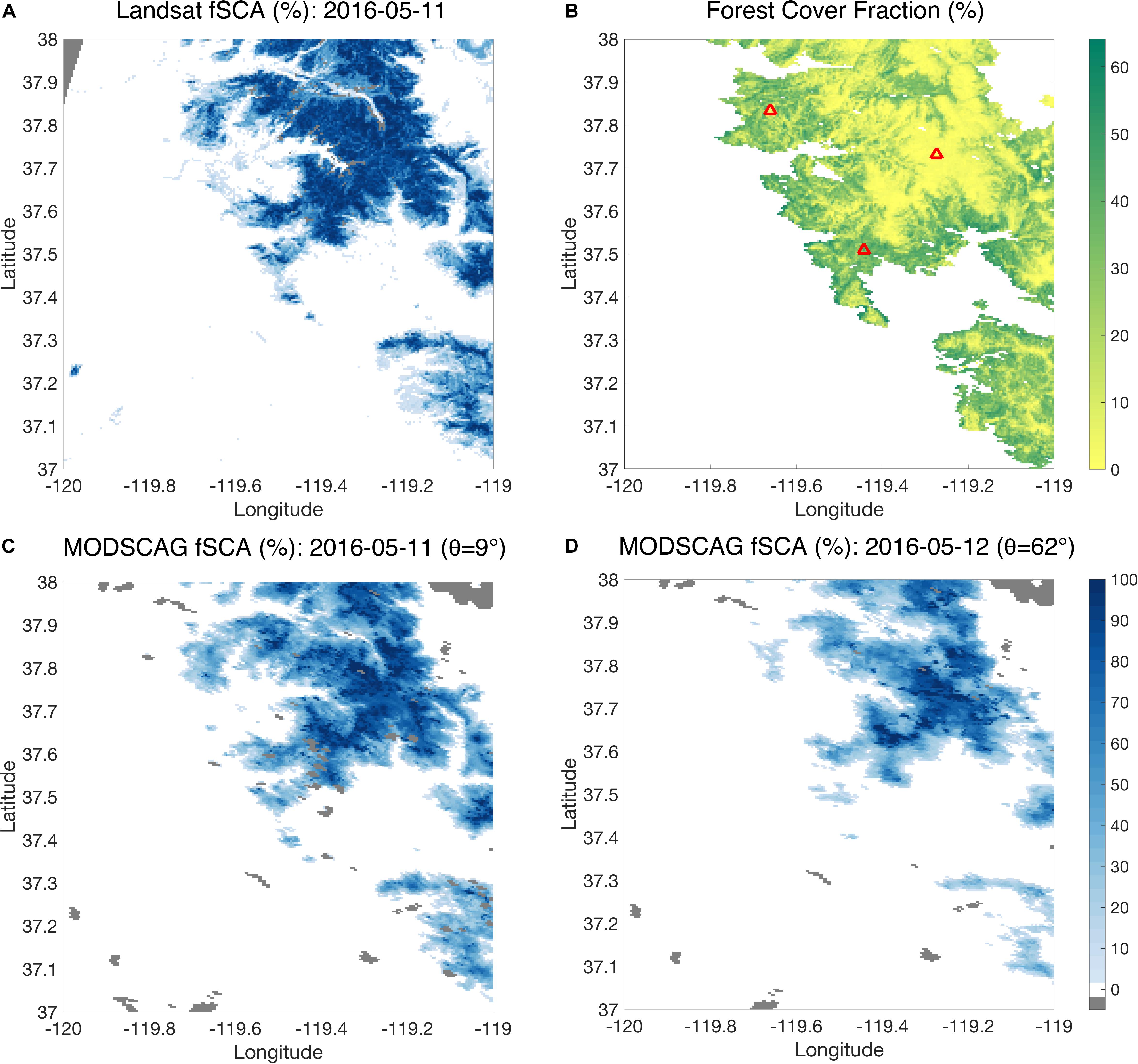
Figure 3. (A) An example of a Landsat fSCA map for a tile covering the Tuolumne River watershed examined herein. (B) Map of forest cover over the tile including three sample points (red triangles) used for illustration in Figure 6. (C) Coincident (within 1 day of Landsat image) MODSCAG fSCA maps at (C) low viewing angle and (D) high viewing angle, illustrating the differences (errors) caused by viewing geometry effects. Specifically, the effect of “pixel elongation” described in the text is apparent in (D). Gray areas in fSCA maps represent non-retrievals.

MODIS-Based fSCA (MODSCAG) Data

The MODIS-based fSCA estimates used herein, were extracted from the MODSCAG product (Painter et al., 2009; using v005 MODIS reflectances)². These estimates were derived from the MODIS sensor (Terra satellite) that are available since 2000 and are distributed on the MODIS sinusoidal tile grid (SIN). The MODSCAG fSCA is also derived from a spectral end-member unmixing approach and is therefore consistent with the Landsat-based fSCA from a retrieval algorithm perspective. We interpolated the MODSCAG products from their nominal resolution of ∼463 m to a regular 16 arcsecond (∼480 m) grid to match the reanalysis and (aggregated) Landsat fSCA resolution. Raw MODSCAG images are screened for clouds using the internal MODIS cloud mask. However, the cloud detection algorithm is generally thought to be less discriminating than the Landsat cloud mask algorithm and hence, based on manual testing, we discard any images with a diagnosed cloud cover greater than 10% to avoid using cloudy pixels that are misclassified as snow.

A key difference between MODIS and Landsat data is that MODIS revisit frequency for a given location is daily. However, the tradeoff for this daily sampling is that unlike Landsat, which is near-nadir looking, MODIS is a scanning sensor such that the daily measurements can have significant off-nadir viewing angles (up to ∼65°) at the outer edge of the swath. A schematic of the implications of the viewing geometry is shown in Figure 4. As the viewing angle increases, the sampled footprint of each pixel elongates, most notably in the scanning (i.e., cross-track) direction. Dozier et al. (2008) provide expressions for along-track and cross-track sampling pixel dimensions as a function of viewing geometry. At the outer edges of the swath, the sampled footprint can become as large 2.5 km in the cross-track direction (Dozier et al., 2008), making it about five times as large as the nominal pixel footprint. Despite this much larger sampled footprint, the reflectance data is regridded and stored on the nominal footprint grid (i.e., at ∼463 m). The implications of this are important, but seldom accounted for in analysis or usage of retrieved MODIS-based fSCA. For example, in the case of forest-covered surfaces in flat terrain (Figure 4A), the general impact is that more of the snow is obscured at larger viewing angles. This can artificially reduce the fSCA from an image at high viewing zenith angle relative to one at low viewing zenith angle. Since the reanalysis framework diagnoses SWE changes from fSCA changes, assimilating such images could lead to erroneous estimates of snow states, where viewing angle variations are (erroneously) ascribed to snow dynamics. Additionally, in the case of complex terrain (Figure 4B), the elongation of sampled footprints can be exacerbated and are not systematic. The larger sampled footprints will sample more of the surrounding terrain, which could have varying levels of snow cover, rock or vegetation making the retrieved fSCA potentially non-representative of the pixel being modeled. To further illustrate this, a sample set of MODSCAG images, within 1 day of the previously discussed Landsat image is shown in Figure 3 and demonstrates how changes in viewing geometry greatly impact the retrieved fSCA. In particular, within 1 day, the viewing angle goes from ∼ 9° to over 60°. The “pixel elongation” in the latter case is evident, while the case closer to nadir compares more favorably to the Landsat image.

FIGURE 4

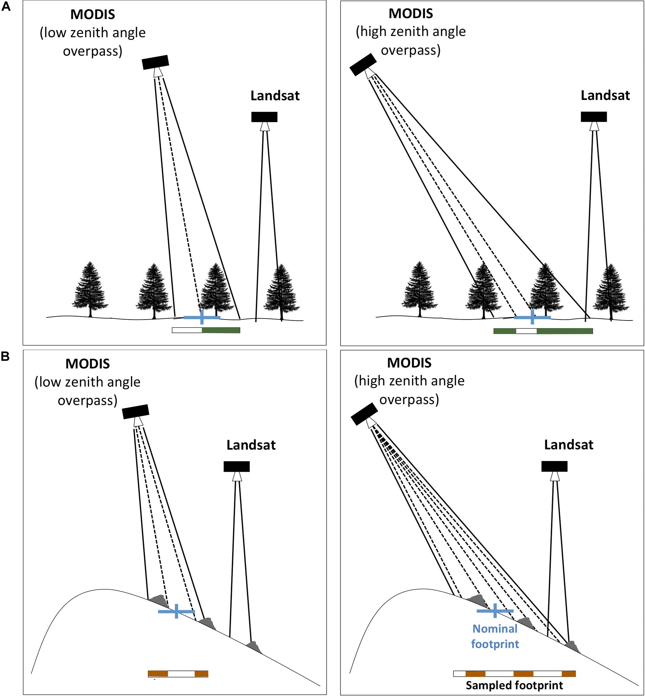
Figure 4. Schematic illustrating the time-varying viewing geometry effects of MODIS on fractional snow covered area (fSCA) retrieval: (A) illustrative impacts of forest cover on sampled footprint at two viewing angles (low zenith angle on left and high zenith angle on right). The blue lines represent a MODIS grid point center (vertical tick) and nominal resolution (horizontal line; ∼463 m), at which the retrieval is provided. The actual sampled footprint is represented by the white rectangle that is filled with white and green representing snow and forest respectively that is actually seen by the sensor within its sampled footprint. In the case shown on the right, for the same snow on the ground, the MODIS sampled footprint will see more forest and therefore less snow. (B) Illustrative impacts of topography and rock outcrops (shown in gray). The actual sampled footprint is represented by the white rectangle that is filled with white and brown (representing snow and rock respectively) within the footprint. The “stretching” of the sampled footprint in the scanning direction will distort the retrieved fSCA that is mapped into the nominal footprint due simply to the viewing angle. In contrast, the Landsat viewing angle does not change.

In the context of DA, the errors caused by viewing geometry should be reflected in the measurement error covariance structure such that more accurate/representative fSCA measurements are trusted more and less accurate/representative measurements are trusted less. Specifically, as the viewing zenith angle approaches zero the measurement error covariance should approach that of the Landsat fSCA, while at higher viewing angles the measurement error covariance should grow. For this relationship, we borrow from the developments of Dozier et al. (2008). In their work, a function based on viewing geometry was used as a weighting function (W) in a least-squares term used to fit splines to the raw MODSCAG data, i.e.:

$$W\left({\mathrm{\theta }}_s\right)=\frac{p^{2}cos\mathrm{\theta }}{p_{\parallel }{p}_{\perp }}(5)$$

where p is the linear pixel dimension at nadir (463 m), θ is the sensor viewing angle, and p_‖ and p_⊥ are the along-track and cross-track pixel dimensions at a non-nadir scan angles (see Dozier et al., 2008 for detailed expressions of these quantities). In weighted least-squares estimation, with assumed Gaussian measurement errors (consistent with the assumptions herein), the weighting function is theoretically proportional to the inverse of the measurement error covariance. Hence we use this theoretical grounding in combination with the above weighting function to specify how measurement error covariance varies with sensor viewing zenith angle:

$$C_V^{MODSCAG}\left(\mathrm{\theta }\right)=\frac{C_V^{MODSCAG}(\mathrm{\theta }=0)}{W(\mathrm{\theta })}(6)$$

where the numerator represents the specified error covariance at nadir (i.e., θ = 0). Based on the formulation in Equation (6), the MODSCAG measurement error covariance values at viewing zenith angles of ∼10°, 20°, and 35°, would be increased by a factor of ∼1.05 ∼ 1.25, and ∼2 respectively. Therefore, from the perspective of the DA framework, off-nadir measurements would be treated as less accurate than nadir measurements, and therefore trusted to a lesser degree (as desired).

MODSCAG Screening, CDF-Matching to Landsat Data, and fSCA Measurement Errors

As illustrated in Figure 3, even at near-nadir viewing angles, there are same-day differences between Landsat- and MODSCAG-retrieved fSCA. While the differences could result from a variety of potential factors (sensor differences, retrieval algorithm differences, and errors associated with the interpolation of the raw MODSCAG data to the modeling resolution) a key factor is likely the differences in scale between the raw reflectances (i.e., 30 m vs. 463 m) used to construct fSCA and the varying viewing angle sampling resolution of MODIS discussed above. The differences in sampling resolution are evident as higher-resolution features are seen in the Landsat image even though the Landsat and MODSCAG fields are both displayed at a resolution of 480 m. As discussed above, the differences become larger as the viewing zenith angle increases (Figure 3D). These systematic differences yield conflicting information in some images that needs to be addressed within the DA framework. We propose to do this in two ways: (1) MODSCAG data are screened to only assimilate those that are below a certain viewing angle threshold (i.e., those with lowest measurement errors) and (2) a CDF-matching algorithm is used to put the screened MODSCAG data on the same footing as the Landsat data. Such CDF-matching approaches are commonly used in DA frameworks where data from multiple sensors are being used (e.g., Reichle and Koster, 2004; Reichle et al., 2007; Liu et al., 2011; Kumar et al., 2015b).

The screening of MODSCAG data is designed to provide additional high-quality information (i.e., at relatively low viewing zenith angles) to supplement cloud-free Landsat data, while excluding those measurements that are most likely to be erroneous (i.e., at higher viewing angles). The viewing angle screening threshold should be treated as a user-specified adjustable parameter depending on the application and domain. We performed sensitivity tests with different screening thresholds and ultimately settled on using viewing angles (θ) less than 20° herein to screen MODSCAG data. As described in more detail below (see Section Spatially-Distributed Estimates Over Tuolumne and the Impact of Using Joint Landsat-MODSCAG Measurements4.1.2), incorporating more MODSCAG observations at higher viewing angles can have negative impacts over using Landsat and high-quality MODSCAG observations. To provide context, Figure 5 illustrates the number of cloud-free Landsat observations (including both Landsat 7 and 8) and MODSCAG observations (for θ < 20°) available over both the Tuolumne and HMA domains in WY 2016. Note that the Landsat measurement pattern is heterogeneous and includes areas where Landsat tiles overlap and areas covered by single tiles (Figure 5, top row). In the tile overlap areas, which happens to include much of the Tuolumne watershed, the number of cloud-free measurements are on the order of 60/year, while in the areas of single tile coverage are on the order of 30/year, with the exception of the southeastern portion of the HMA domain, where monsoon-driven clouds tend to reduce the number of available Landsat images. When MODSCAG images are screened by viewing angle, there is a similar pattern of high density measurements in the near-nadir MODIS overpass track locations and lower density in between tracks (Figure 5, middle row). When the Landsat and screened MODSCAG data are combined, the number of assimilated measurements are at least 40/year over both domains (Figure 5, bottom row). The tradeoffs between Landsat-only vs. incorporating additional MODSCAG observations are discussed below.

FIGURE 5

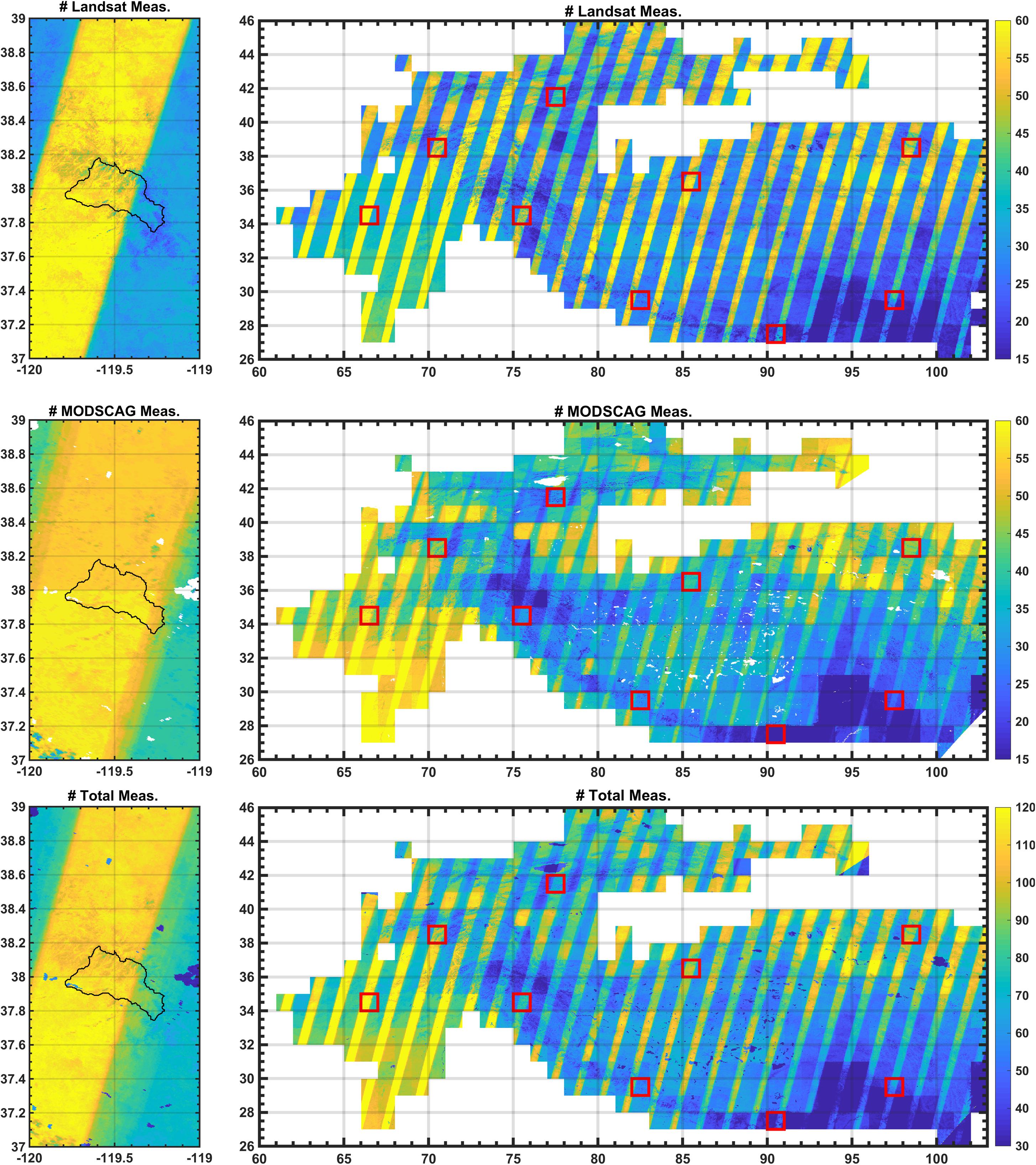
Figure 5. (Top row) Number of available cloud-free Landsat measurements over Tuolumne (left) and HMA (right) domains for WY 2016. (Middle row) Number of available cloud-free MODSCAG measurements (screened for viewing zenith angles θ < 20°) over Tuolumne (left) and HMA (right) domains for WY 2016. (Bottom row) Total number of available cloud-free Landsat and screened MODSCAG measurements over Tuolumne (left) and HMA (right) domains for WY 2016.

After screening, the CDF-matching algorithm used herein is applied as follows: Over the shared observation period of 2000–2017, all Landsat and screened MODSCAG images within 2 days of each other are collected. Each set of data (including only snow-covered cases) is used to create a pixel-specific empirical CDF for both Landsat and MODSCAG fSCA. The raw CDFs are discretized and saved at specified percentiles between 0 and 1. The two discretized CDFs (i.e., F_MODSCAG(fSCA) and F_Landsat(fSCA)) are then used to map the raw (screened) MODSCAG data to the equivalent Landsat basis using CDF-matching, i.e.:

$$fSC{A}_{meas,MODSCAG}^{\prime }=F_{Landsat}^{-1}\left[F_{MODSCAG}(fSC{A}_{meas,MODSCAG})\right](7)$$

where $fSC{A}_{meas,MODSCAG}^{\prime }$ is the transformed (CDF-matched) MODSCAG measurement. Because the empirical CDFs are discretized, linear interpolation is used in the mapping shown in Equation (7).

An example of the CDF-matching procedure is shown in Figure 6. The derived CDFs (where the MODSCAG CDFs are generated using only screened measurements) for three pixels are shown (middle column), where the three are chosen to be illustrative of three different forest-cover cases (see Figure 3B): (1) a pixel that is essentially unforested (f_forest = 1%) and in a clearing, (2) a pixel that is moderately forested (f_forest = 46%), but surrounded by less forest cover, (3) a pixel that is nearly unforested (f_forest = 4%), but surrounded by high forest cover fraction pixels. For the first pixel, where there is minimal forest at the pixel and over its surroundings, the two CDFs are very similar such that the CDF-matching generates only limited changes to the raw (screened) MODSCAG data. In the second case the CDF-matching leads to a reduction in the raw MODSCAG fSCA. This is likely because MODIS samples neighboring less-forested pixels introducing a positive bias relative to the Landsat fSCA. Finally, in the last case, the CDFs are significantly different where the CDF-matching leads to a significant increase in the raw MODSCAG fSCA. This can be explained by the pixel being surrounded by more highly forested pixels that reduce the fSCA when sampled off-nadir by MODIS. It should be noted that the arguments regarding forest cover are only one factor and that the reality is more complicated due to the complex terrain that will also lead to heterogeneity in the underlying true fSCA field that gets sampled differently by MODIS and Landsat. When applied pixel-wise to the full image the result is a transformed MODSCAG image that is more consistent with the Landsat image (Figure 6). For the three example pixels the time series of fSCA is also shown. By design the fSCA time series using the Landsat and transformed (screened) MODSCAG are more consistent with each other and amenable to simultaneous assimilation using the snow reanalysis approach. Together, the Landsat and CDF-matched (screened) MODSCAG data make up the vector fSCA_meas that appears in Equation (3).

FIGURE 6

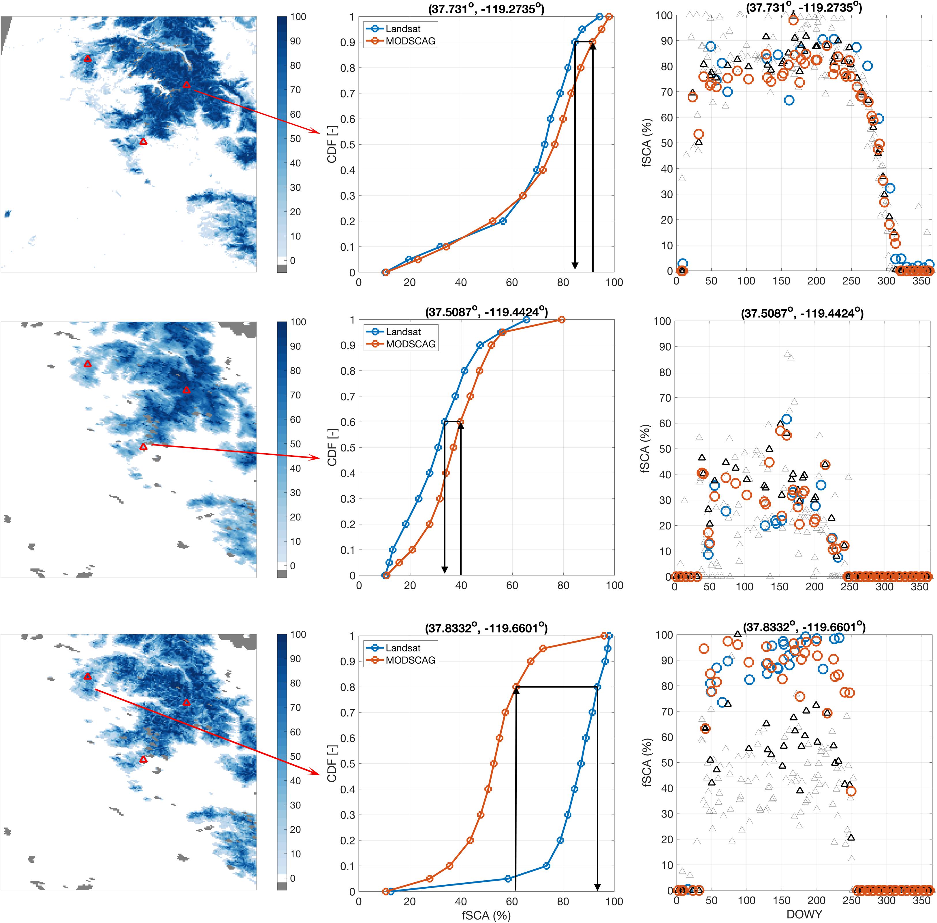
Figure 6. (First column) Sample (WY 2016) images of fSCA estimates from Landsat (top), raw MODSCAG (middle) and CDF-matched MODSCAG. (Second column) Empirical CDFs for: Landsat (blue) and screened (i.e., with viewing zenith angles θ < 20°) MODSCAG (orange) for the three locations illustrated by red triangles in the first column. (Third column) Sample time series for WY 2016 for the three locations showing the: Landsat (blue), raw MODSCAG [black (θ < 20°)/gray (θ > 20°) triangles], and CDF-matched MODSCAG corresponding to screened measurements (orange circles). The open circles (i.e., Landsat and screened/CDF-matched MODSCAG) are those measurements that are assimilated in the snow reanalysis method.

Finally, the measurement error covariance for both Landsat and MODSCAG must be specified [Equations (4) and (6)] for use in the reanalysis framework. Based on our previous work (Cortes et al., 2014) the standard deviation of Landsat fSCA error at ∼100 m resolution was found to be ∼15%. Therefore the error is expected to range between 3 to 15% when Landsat fSCA is aggregated to ∼480 m as done herein, depending on the independence of sub-grid errors. Based on analysis over Tuolumne it was found that the Landsat fSCA error standard deviation at ∼480 m was ∼10%. This value is used to populate the diagonal of $C_V^{Landsat}$, where for simplicity it is assumed that errors between different image acquisitions are uncorrelated (zero-valued off-diagonal terms). The MODSCAG nadir error covariance in Equation (6) was estimated based on the Landsat measurement error discussed above and the disagreement between CDF-matched MODSCAG data and Landsat data. Specifically, assuming the Landsat and MODSCAG errors are independent, it can be shown that the sum of Landsat and MODSCAG measurement error variances are equal to the mean squared difference between Landsat and CDF-matched MODSCAG fSCA estimates. Based on this analysis over Tuolumne, it was found that the CDF-matched MODSCAG error covariance at near-nadir is ∼15%, which is used populate the diagonal of $C_V^{MODSCAG}$ using the near-nadir value and Equation (6) based on viewing geometry of individual acquisitions.

Model Input Data

MERRA2 meteorological inputs

The LSM-SDC model requires hourly meteorological inputs. In our previous work over the Sierra Nevada we used the NLDAS-2 dataset (Cosgrove et al., 2003; Xia et al., 2012) which is available at 0.125° × 0.125° over CONUS. To extend the methods for global applicability and usage over the full remote sensing record we chose to use the MERRA-2 dataset (Gelaro et al., 2017). MERRA-2 is available globally from 1980-present at a horizontal resolution of 0.5° × 0.625° and is itself a large-scale reanalysis, which benefits from a significant amount of atmospheric DA including atmospheric motion vectors, surface winds, temperature and ozone profiles, and microwave and infrared sounding radiances. For the purposes of this work we specifically used the hourly 2D surface fields (Global Modeling and Assimilation Office [GMAO], 2015a,b,c) that provide reference-level precipitation (“PRECTOT”), incoming solar radiation (“SWDGN”), air temperature (“T2M”), specific humidity (“QV2M”), surface pressure (“PS”), and wind speed (“U10M” and “V10M”). For the purposes of forcing the LSM-SDC at each pixel, the non-precipitation MERRA-2 data are downscaled as described above in Section “Bayesian Snow Reanalysis Framework,” while the precipitation is perturbed as shown in Equation (1).

Ancillary inputs and parameter uncertainty

The remaining ancillary inputs needed for the modeling and assimilation framework were drawn from globally available datasets or based on previous work. Topographic data was taken from the 30 m (1 arcsecond) resolution Shuttle Radar Topography Mission (SRTM) DEM (Farr et al., 2007). Any gaps in SRTM coverage were filled by the Advanced Spaceborne Thermal Emission and Reflection (ASTER) DEM (NASA, 2001). The DEM was used to determine secondary variables used by the forcing downscaling scheme or LSM-SDC (e.g., slope, aspect, sky-view factor). Forest fraction (f_forest), which is used in the measurement model Equation (2), was taken from the Landsat continuous vegetation field dataset (Sexton et al., 2013). Landcover maps were specified based on the 1 km Advanced Very High Resolution Radiometer (AVHRR) global land cover classification database (Hansen et al., 2000). The glacier mask was extracted from the GLIMS glacier dataset (GLIMS and NSIDC, 2018). For the purposes of the reanalysis, all open water surfaces and glacierized areas are masked out from the reanalysis domain to focus on seasonal snow over land. A final ancillary input that is used in the measurement model Equation (2) is the fraction of perennially exposed rock (f_rock) that does not typically get snow covered. While no standard dataset is available for estimating this parameter, we use the combined information in the f_forest estimates and historical Landsat fSCA data to estimate it. In particular, based on manual testing, we assume that the 95th percentile of Landsat fSCA (over the period 2000–2017) for each pixel (which is derived as part of the CDF-matching algorithm described above) is representative of the maximum observed fSCA [fSCA_max(x)]. Using a higher percentile was found to allow for the possibility of including misidentified clouds as snow to contaminate the estimate. Based on this estimate of fSCA_max, any difference between that value and 100% is assumed to be the result of obscuring forest cover and exposed rock (where grass, shrubs or other low-lying vegetation will typically be buried by snow at some point during the joint Landsat-MODIS-era used to construct the CDFs). Hence the estimate of perennially exposed rock fraction is given by:

$$f_{rock}\left(x\right)=1-f_{forest}\left(x\right)-fSC{A}_{max}\left(x\right)(8)$$

Testing indicated that the method is not very sensitive to specification of f_rock, however it is introduced to maintain consistency between the predictions and measurements of fSCA in the measurement model.

Based on the underlying DEM and Landsat fSCA dataset, the reanalysis could be run at spatial resolutions as high as 30 m. However, for simplicity in assimilating both Landsat and MODSCAG data and for computational savings in applying the method over large domains (e.g., HMA) all ancillary data were resampled to a baseline model resolution of ∼480 m (16 arcsecond) defined by aggregating the underlying DEM. Future work will aim to apply the multi-resolution approach of Baldo and Margulis (2017, 2018) to the joint assimilation of Landsat and MODSCAG.

The final set of input parameters needed for application of the method are the specified PDFs and uncertainty parameters that control the random variables used in the reanalysis framework. The set of random variables are the same as in previous work (Margulis et al., 2016a), namely those controlling the precipitation, air temperature, dewpoint temperature, and incoming shortwave radiation meteorological forcings, the subgrid coefficient of variation parameter (β) in the SDC model, and the snow albedo scaling parameter (C_VIS). The uncertainty model distributions and relevant parameters are shown in Table 1.

TABLE 1

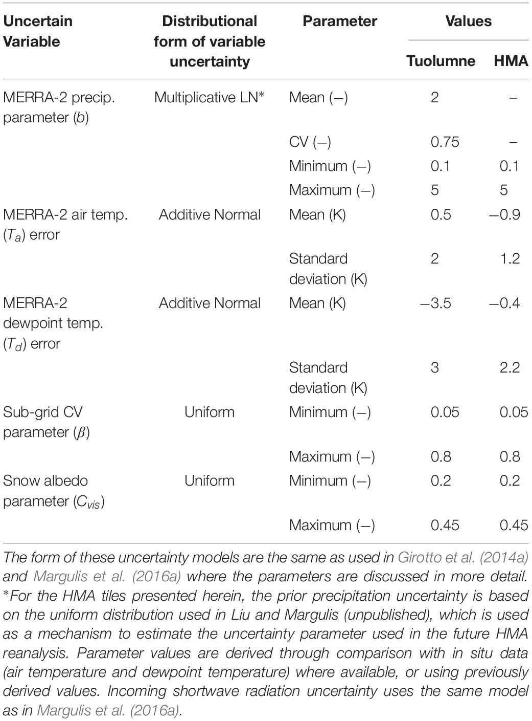
Table 1. Parameters used in the specification of prior uncertainty in key snow model inputs.

Verification Data: Airborne Snow Observatory (ASO) Data

The ASO dataset³ (Painter et al., 2016), which provides multi-temporal Lidar-derived snow depth images and SWE estimates (using model-based and/or in situ snow density) over Tuolumne, was used to verify the method. The 50 m ASO product was re-gridded to the reanalysis modeling resolution of ∼480 m for comparison. We used data from WYs 2015, 2016, and 2017, which span a historically dry, a relatively normal, and a historically wet year respectively. The number and dates of ASO images from these 3 years are shown in Table 2.

TABLE 2

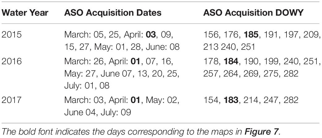
Table 2. Airborne Snow Observatory (ASO) acquisition dates over Tuolumne River watershed and their corresponding day of water year (DOWY) values.

Results and Discussion

Verification Using ASO Data Over Tuolumne River Watershed

Illustrative Results at the Grid Cell

The snow reanalysis method was evaluated using ASO data over Tuolumne for WYs 2015 (dry), 2016 (near-average), and 2017 (wet). Figure 7 is used to illustrate how the method works at the grid cell level using four sample locations at high-elevation in the Tuolumne watershed (Figure 1A). The basic procedure is as described above: (i) the forward model generates an ensemble prior estimate (of equally likely replicates) for fSCA and SWE over the full WY (shown in red), (ii) the PBS update equation generates posterior weights reflecting how well individual replicates fit the Landsat and MODSCAG fSCA measurements (open circles and squares respectively), (iii) the posterior weights are used to generate a posterior ensemble estimate for fSCA and SWE (shown in blue). The posterior SWE estimates are then compared to the independent ASO SWE estimates (open triangles).

FIGURE 7

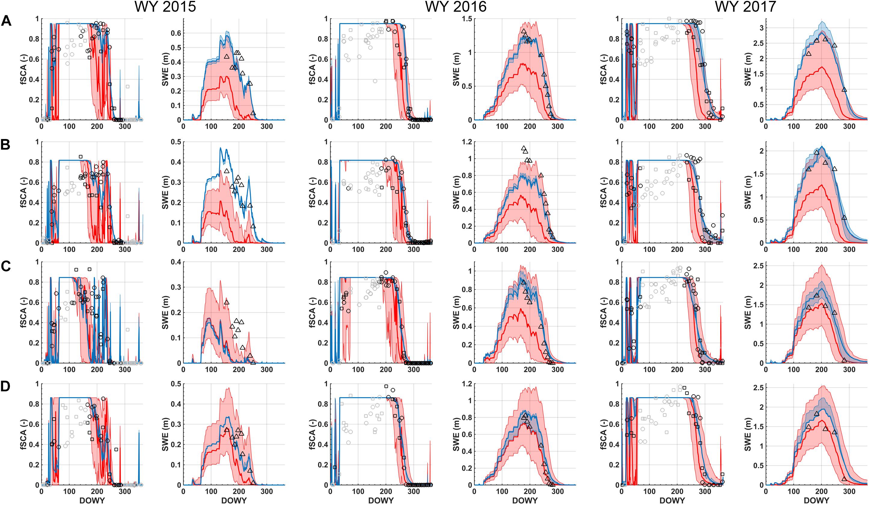
Figure 7. (A) Prior (red) and posterior (blue) predicted fSCA and grid-averaged SWE for each WY corresponding to location #1 shown in Figure 1. The ensemble estimates are represented by the: median (solid line) and inter-quartile range (shaded region). Assimilated fSCA measurements are shown as open circles (Landsat) and CDF-matched MODSCAG (open squares). The fSCA measurements shown in gray are those that do not contribute to the update (since the prior ensemble spread is zero). The independent ASO SWE estimates are shown as open triangles. Panels (B–D) are the same but for location #2 to #4 shown in Figure 1 respectively.

Figure 7A illustrates this for location #1 in the northwest of Tuolumne for WYs 2015-2017. The prior ensemble median SWE for each of the 3 years at this location peaks at ∼0.3, 0.75, and 1.75 m respectively with a large uncertainty bound (representing the inter-quartile range) around the median. The uncertainty bounds are the result of the input uncertainties (i.e., related to snowfall, other meteorological inputs, snow albedo, and sub-grid coefficient of variation parameter) that are propagated through the forward model. The SDC in the model is used to represent the evolution of predicted fSCA as seen by the satellite (fSCA_pred), which is typically highly variable early in the water year, saturates at fSCA_max (after enough snow has accumulated) and then shows depletion during the spring/summer months. The timing and rate of depletion is a function of the underlying SWE and melt rates during ablation. Any discrepancies between the predicted and observed fSCA are then used to generate the posterior weights used to derive the posterior SWE estimates. In all three WYs at location #1, the prior ensemble median for fSCA is lower (i.e., earlier depletion) than the observations. This causes those ensemble members with higher values of fSCA to be weighed more heavily, resulting in the posterior fSCA distribution, which, by construct, fits the observed fSCA better than the prior. The same update is applied to the SWE ensemble, resulting in an increase in the posterior ensemble median SWE (and a reduction in posterior uncertainty). The resulting posterior ensemble median SWE peaks at ∼0.6, 1.25, and 2.75 m respectively across the three WYs, where the increased SWE is implicitly more consistent with the fSCA depletion time series. The ASO SWE estimates are shown in comparison to the prior and posterior SWE in each WY. For this particular location, the posterior estimates of SWE are in better agreement with the ASO estimates than the prior estimates are.

Figures 7B–D illustrates the same results for the other three sample locations (Figure 1). The overarching results are qualitatively the same as for location #1 with some variations. Generally speaking, the prior estimates of fSCA underestimate the observed values, which lead to an increase in the posterior SWE estimates relative to the prior. One exception to this is location #3 (Figure 7C) in WY 2015, where the prior fSCA predictions are relatively consistent with the fSCA measurements such that the prior and posterior ensemble median SWE are similar (with a reduced uncertainty in the posterior). WY 2015 was unusual in that it was a historically dry snow year (Margulis et al., 2016b) and therefore led to early melt-out followed by intermittent snowfall and melt events later in the year, compared to the more typical single melt out seen in WYs 2016 and 2017 (seen across all four locations). Hence the fSCA depletion-SWE relationship is much noisier in WY 2015. For location #3 in WY 2015, the prior and posterior show lower SWE than the ASO estimates. At that same location in other years, the posterior estimates of SWE are in much better agreement with ASO SWE. Another case that is worth pointing out is location #2 (Figure 7B) in WY 2016. While the posterior fSCA distribution is in reasonable agreement with the measurements (by construct), and there is a large increase in the posterior SWE estimates relative to the prior, the posterior peak SWE estimates are less than those estimated by ASO. To the extent that the ASO SWE estimates are closest to the true SWE values, the fact that the posterior peak SWE underestimates SWE, while matching the observed fSCA depletion time series, indicates potential errors in the modeled melt fluxes. Such errors are most likely attributable to the coarse (MERRA-2) meteorological inputs that are downscaled and used in the model.

Another point to make, that is illustrated in Figure 7, has to do with the fSCA observations that contribute to the posterior update. While all fSCA measurements shown are used in the Bayesian update Equation (3), not all will contribute meaningful information with respect to the posterior. In particular, in cases where the prior ensemble spread in predicted fSCA is negligible, which typically happens either when all replicates saturate at fSCA_max in the mid- to late-accumulation season or converge to zero after ablation, there will be no differential penalty (with respect to those measurements) for one ensemble member over another since all will have exactly the same discrepancy with measurements (likelihood) at those times. This is illustrated in Figure 7, where those measurements that contribute meaningful information are shown in black, while those without meaningful contribution are shown in gray. The “non-informative” measurements primarily occur during mid- to late-accumulation season, when fSCA-SWE information is expected to be lowest, which is implicitly being confirmed via the fact that that ensemble spread in predicted measurements is negligible. During the accumulation season, fSCA retrievals tend to be noisier due to lower solar zenith angles, increased terrain shading, potential for cloud vs. snow misclassification, and other factors. The seemingly large differences during that period are attributed to these factors. To the extent that some of those measurements may be measuring real snow dynamics, this would indicate weakness in the SDC model which is invariably a simplification of sub-grid snow cover dynamics that is arguably best suited for capturing the main ablation season depletion. The end result is that high information content measurements during the ablation season are those that primarily contribute to the update. Pixels that are less seasonal (more intermittent fSCA) are more likely to have less information in the fSCA time series that can be used to update the prior.

Spatially Distributed Estimates Over Tuolumne and the Impact of Using Joint Landsat-MODSCAG Measurements

The prior and posterior estimates were compared to the spatial estimates from ASO to more fully characterize the performance of the method. Figure 8 illustrates the spatial SWE fields for the ASO estimate closest to April 1st in each WY compared to the prior and posterior ensemble median fields and the difference fields relative to ASO estimates on those days. WY 2015 was a historically dry year so that SWE was relatively low on DOWY 185 (generally less than 0.5 m and limited primarily to the highest elevations of the Tuolumne watershed). The ASO SWE field is well correlated with the posterior with a spatial pattern correlation of ∼0.84 compared to ∼0.55 with the prior. The posterior shows a small mean difference (MD; less than 1 cm) with a root-mean-squared difference (RMSD) of ∼ 5 cm, while the prior has a MD and RMSD of ∼−5 cm and ∼9 cm, respectively. In WYs 2016 and 2017 most of the watershed was covered by snow near April 1st (DOWYs 184 and 183 respectively) with SWE values in some locations exceeding 1.2 and 2.5 m respectively. In both years the posterior had a much larger pattern correlation (0.81 and 0.86 respectively) with ASO than does the prior (0.59 and 0.55 respectively). The mean differences are largest in WY 2016 where the posterior has an MD of ∼−12 cm compared to the prior MD of ∼−23 cm. The prior shows large negative differences at high elevations and positive differences at low elevations. The posterior reduces these differences, but still exhibits negative differences at high elevations. We hypothesize that this is due to errors in the downscaled MERRA-2 forcing inputs. Sensitivity tests (not shown) found that when using the higher-resolution NLDAS-2 forcing in this year, the differences were smaller. This highlights that, where available, higher resolution forcing inputs may provide benefit due to the need for less downscaling (although tests in WYs 2015 and 2017 showed similar performance when using NLDAS-2 and MERRA-2 forcing). In WY 2017 the low- vs. high-elevation contrast in prior SWE differences was amplified compared to WY 2016. So while the prior MD was relatively low (∼−6 cm), this was primarily due to the large positive and negative errors canceling out rather than an indicator of a good estimate. This is confirmed by the large prior RMSD (∼63 cm). The posterior reduced the prior errors with a MD of ∼ 2 cm and RMSD of 39 cm.

FIGURE 8

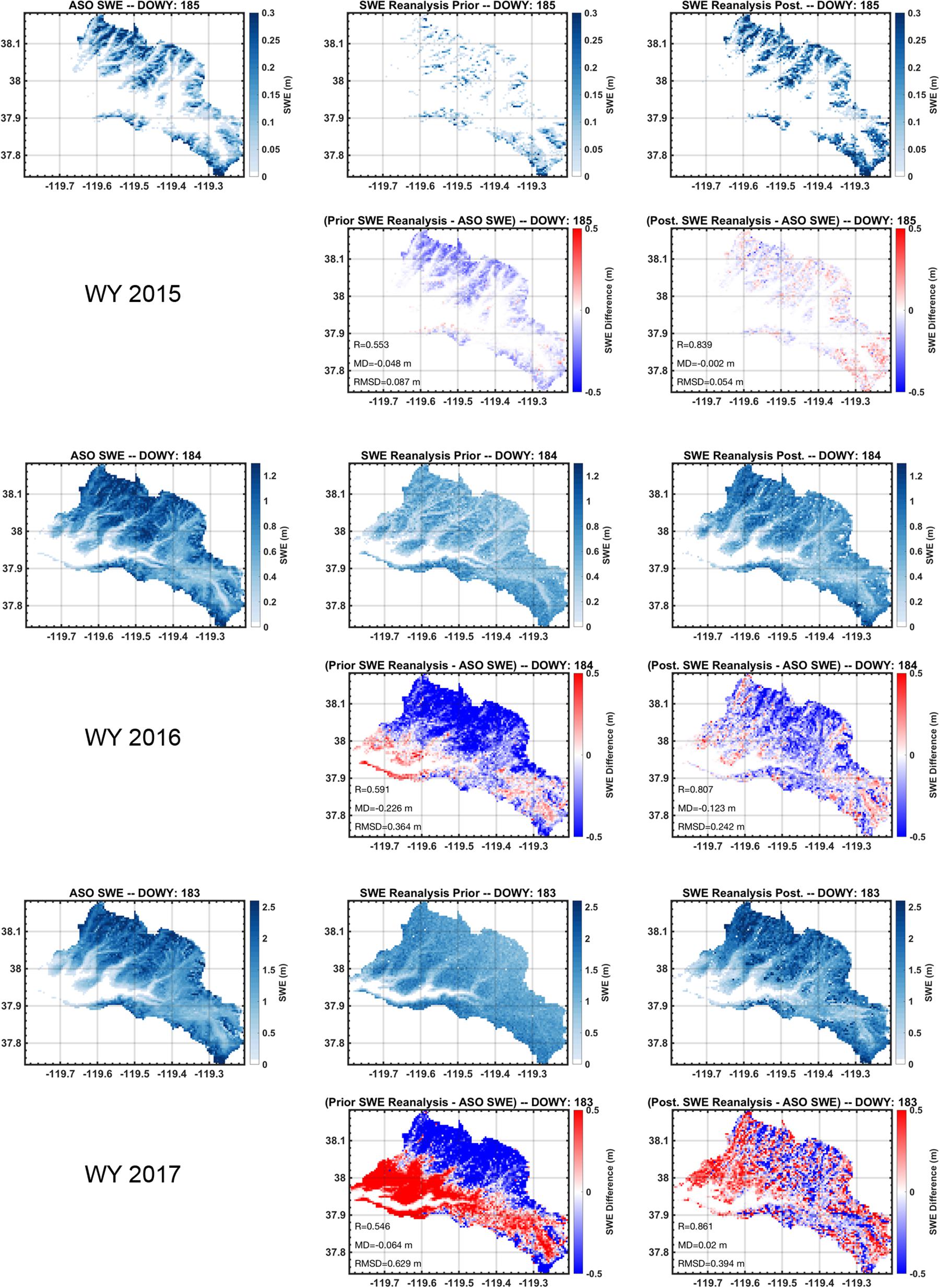
Figure 8. Comparison of reanalysis results to ASO SWE estimates nearest April 1st in each verification year (WYs 2015–2017). For each WY, the ASO SWE estimates are shown in the left panel followed by the (ensemble median) prior and posterior SWE estimates. Difference fields are shown below the prior and posterior estimates to illustrate the differences relative to ASO SWE. The spatial correlation (R), mean difference (MD) and root-mean-squared difference (RMSD) relative to ASO SWE estimates are shown in the prior and posterior difference panels.

Beyond the SWE fields near April 1st, a similar comparison was performed for all of the ASO flight days shown in Table 2. For each day, the prior and posterior spatial correlation, MD and RMSD are shown side-by-side in Figure 9. For the spatial correlation (top row), the posterior uniformly outperforms the prior. The posterior mean (range) in correlation for each WY is 0.80 (0.65–0.87), 0.79 (0.69–0.84), and 0.82 (0.71–0.87). In contrast the prior mean (range) in correlation for each WY is 0.55 (0.50–0.61), 0.59 (0.55–0.64), and 0.51 (0.28–0.62). On average, the posterior correlation coefficient values are 45% higher than the prior values. In terms of MD, the posterior performs best in WYs 2015 and 2017 where the magnitude of MD values are generally less than 5 cm in 2015 and less than 10 cm in 2017. The largest posterior MD values are in WY 2016, where negative MD values of 10–20 cm are seen in the late accumulation season. With respect to RMSD, the posterior estimates are generally comparable to or considerably better than the prior across all three WYs. The posterior mean (range) in RMSD for each WY is ∼7 cm (4–11 cm), ∼15 cm (4–28 cm), and ∼37 cm (26–43 cm). The prior mean (range) in RMSD for each WY is ∼ 10 cm (4–13 cm), ∼22 cm (5–40 cm), and ∼ 54 cm (32–67 cm). On average, the posterior RMSD values are 29% lower than the prior values.

FIGURE 9

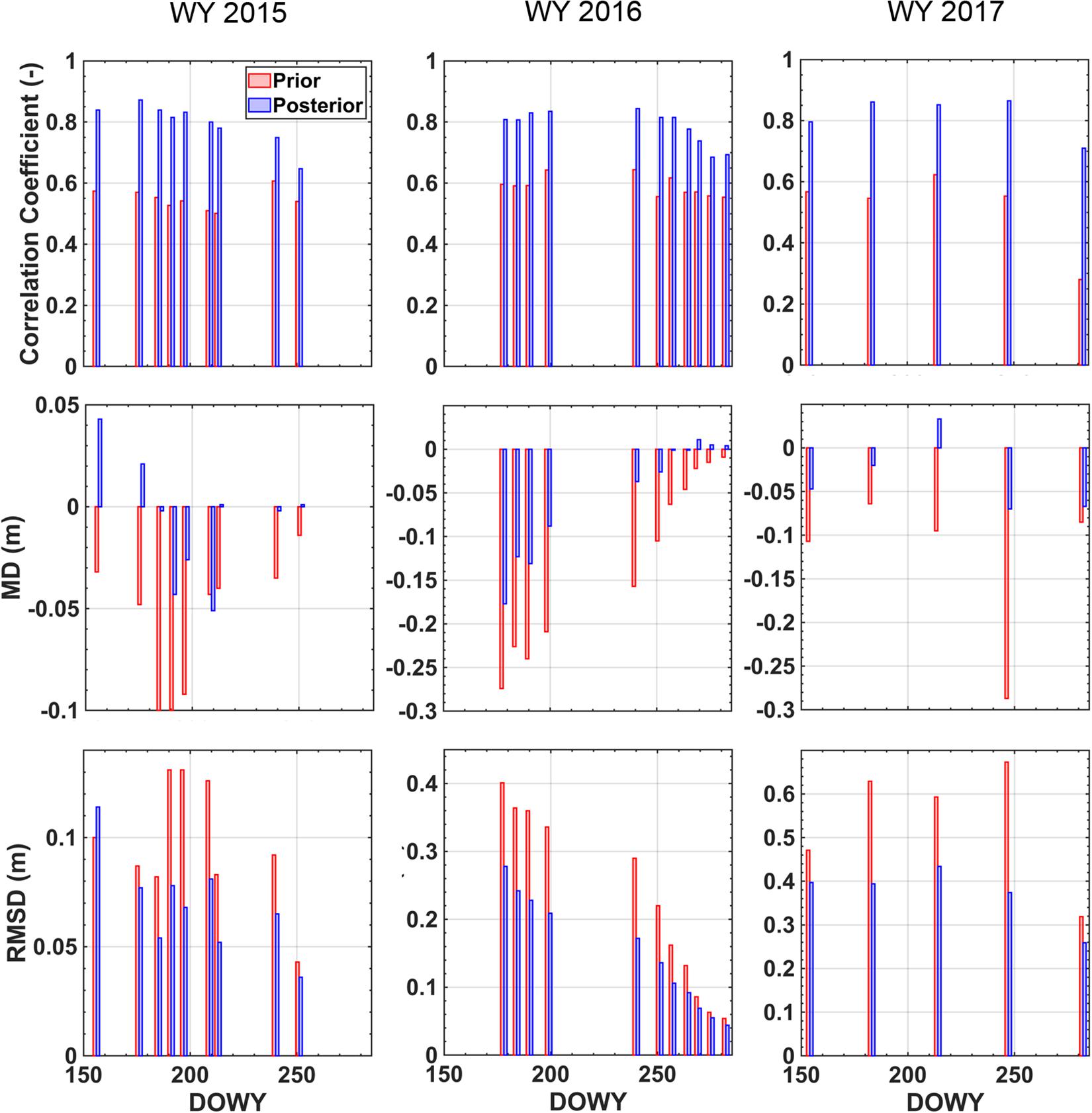
Figure 9. Comparison of ASO SWE estimates to the prior and posterior SWE estimates for each WY (organized in columns) as characterized by the spatial pattern correlation (top row), the mean difference (middle row), and root-mean-squared difference (bottom row). Result for the prior and posterior are shown in red and blue respectively.

To justify the MODSCAG screening method (θ < 20°) used in the results presented above and below, a sensitivity analysis was done for several different assimilation cases over the Tuolumne watershed (Table 3). Specifically, we tested cases with Landsat-only, MODSCAG-only, joint Landsat-MODSCAG and additional cases where the Landsat data was subsampled. The latter cases were examined because Tuolumne happens to be in an area where Landsat tiles overlap, such that it is not representative of the more general (single tile) case. For this reason and to mimic locations with more cloudy conditions, the subsampled Landsat cases used every third Landsat measurement (i.e., so that pixels have ∼20 measurements/year). All assimilation cases outperform the prior across all WYs, indicating the benefit of the additional information contained in the fSCA measurements. The Landsat-only case with all measurements generally performs the best. In particular the spatial correlation for the full Landsat-only case is highest across all WYs, which is attributed to the higher spatial resolution of the raw Landsat data which better resolves spatial snow patterns (Figure 3) compared to MODSCAG. Of the assimilation cases, the (screened) MODSCAG-only case performs the worst, while the joint full Landsat + MODSCAG case results fall between the two end-members. The performance of the Landsat-only case is attributed in part to the fact that Tuolumne happens to benefit from being where Landsat tiles overlap and therefore has a significant number (∼60/year) in a given WY. This is confirmed for the subsampled Landsat-only case, where most error metrics show degradation of performance relative to the full Landsat-only case. Aside from the spatial correlation coefficient, the joint subsampled Landsat + MODSCAG case performs comparably (and in some metrics, i.e., MD and RMSD in WYs 2015 and 2016, outperforms) the subsampled Landsat-only case. We interpret this to reflect the fact that in the general case with single Landsat tile coverage and the potential reduction of measurement number due to clouds, there is some benefit to using screened (and CDF-matched) MODSCAG data. Moreover, the degradation when adding the screened MODSCAG data to even the full Landsat-only case is relatively small. So including MODSCAG data provides added benefit in regions that may be subject to limited Landsat data and provides relatively limited degradation where Landsat data is plentiful. Hence all other results presented herein are for the joint Landsat + MODSCAG case with a screening threshold parameter of θ < 20°.

TABLE 3

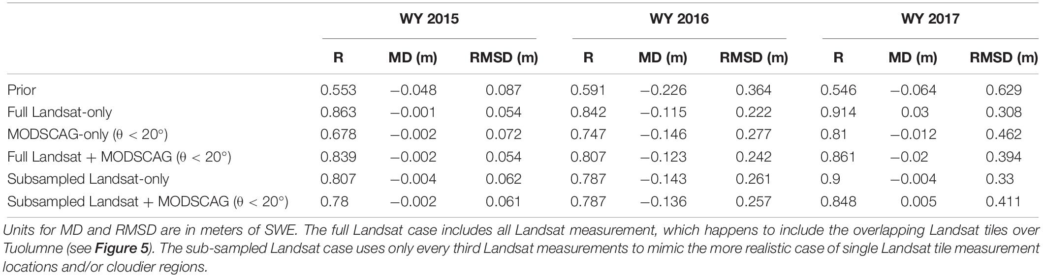
Table 3. Analysis of SWE error metrics (Correlation coefficient: R, Mean Difference: MD, Root Mean Squared Difference: RMSD) for Tuolumne River watershed relative to ASO SWE for ASO measurement DOWY nearest April 1st (see Table 2) for the prior model case and different fSCA assimilation cases.

In summary, the comparison of reanalysis results to independent spatially distributed estimates from ASO provides confidence that the method is able to produce reasonable posterior estimates. All of the inputs used in these results are available globally and thus allow the method to be applied in remote areas where such verification data does not exist.

Sample Results Over HMA Tiles

The primary motivation of the development of the method is to make it applicable to the HMA domain where information on spatially distributed seasonal SWE is extremely limited. Ongoing work is being performed to develop an HMA snow reanalysis dataset for the whole domain shown in Figure 1B, but here we provide some illustrative results for the 9 test tiles examined in Liu and Margulis (unpublished). That work focused on the use of the reanalysis method for deriving estimates of MERRA-2 precipitation uncertainty. Herein we highlight posterior SWE estimates derived for the 9 test tiles, with a focus on the climatological characteristics of peak SWE over WYs 2000-2017. A more thorough and quantitative analysis of domain-wide SWE and its space-time variability will be forthcoming when the HMA snow reanalysis is completed.

Maps of Posterior Peak SWE Climatology in HMA Test Tiles

The reanalysis method provides daily SWE estimates at each pixel over the 18-year application period (WYs 2000–2017). From this we can derive the peak SWE maps for each WY. To first illustrate this for a single tile, the annual map of pixel-wise peak SWE for tile (38°N, 70°E) is shown in Figure 10 (for reference its DEM is shown in Figure 1). The maps are designed to show the seasonal snowpack, i.e., pre-identified glaciers and water bodies are masked out (gray pixels). Some seasonal snow pixels may carry-over snow from 1 year to the next (typically in wet years) and some pixels that are not identified by the glacier mask may in fact be glaciers. To attempt to focus on the climatology of pixels that represent seasonal snow, those pixels with a minimum to maximum SWE ratio (where non-zero represents carry-over SWE) greater than 1% in more than 14 out of the 18 WYs are also masked out. This is an arbitrary threshold, but one designed to allow for the fact that some seasonal snow pixels may have carry-over SWE in many years, but should not in every year if they are indeed seasonal. The combined mask tends to be at the highest elevations (Figure 10). Also note that the pixel-wise peak SWE represents the peak at each grid cell across the WY and is therefore not tied to a particular day, but instead represents the amount of total maximum seasonal snowpack storage across the tile. The individual WY maps show some consistent patterns as well as inter-annual variability in peak SWE (Figure 10). For this particular tile, the maximum SWE is generally on the fringes of glacier pixels, with lower values in the valley regions. In terms of inter-annual variability, WYs 2016, 2004, and 2010 represented the minimum, median, and maximum tile-averaged annual peak SWE years.

FIGURE 10

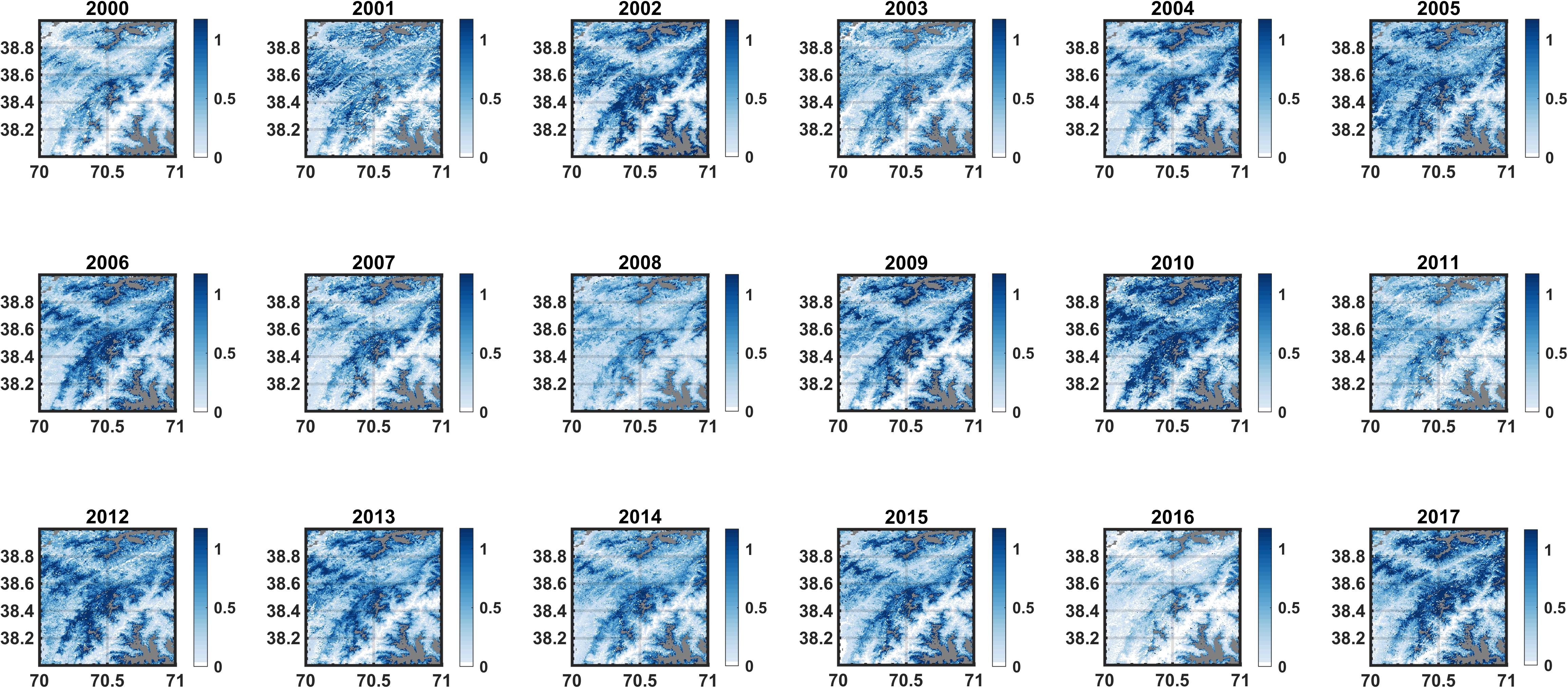
Figure 10. Maps of annual (WYs 2000–2017) pixel-wise peak SWE (in meters) for tile (38°N, 75°E). The gray pixels represent those masked out as pre-identified glaciers, likely glaciers (i.e., pixels with persistent carry-over SWE in more than 14 out of 18 years), or open water bodies. For reference, the DEM of this tile is shown in Figure 1.

The annual maps for each test tile were compiled into a single climatology map as shown in Figure 11. The maps capture the large-scale variations across the HMA domain as sampled by the tiles, with the largest SWE values generally occurring in the tiles (34°N, 75°E) and (38°N, 70°E), intermediate SWE values in tiles (41°N, 77°E), (34°N, 66°E), (29°N, 82°E), (27°N, 90°E), and (29°N, 97°E) and the lowest values occurring in tiles (36°N, 85°E) and (38°N, 98°E). The largest glacierized areas (i.e., with diagnosed persistent carry-over snow) occur in (41°N, 77°E), (34°N, 75°E), (29°N, 82°E), (27°N, 90°E), and (29°N, 97°E). In each tile there is significant spatial variability with the largest values generally occurring, as expected, in the high-elevation regions (see Figure 1 for tile DEMs). Beyond the broad correlation with elevation, peak SWE patterns also show more localized spatial patterns likely indicative of orographic and other effects. One such example is in tile (34°N, 66°E), which largely experiences winter westerlies driving snowfall, and shows what appears to be a strong orographic/rain-shadow in the northeastern portion of the tile where a valley exists to the northeast of a high mountain range. The windward side of the mountain range is where some of the largest peak SWE values are seen, with much lower values on the leeward side and in the leeward valley.

FIGURE 11

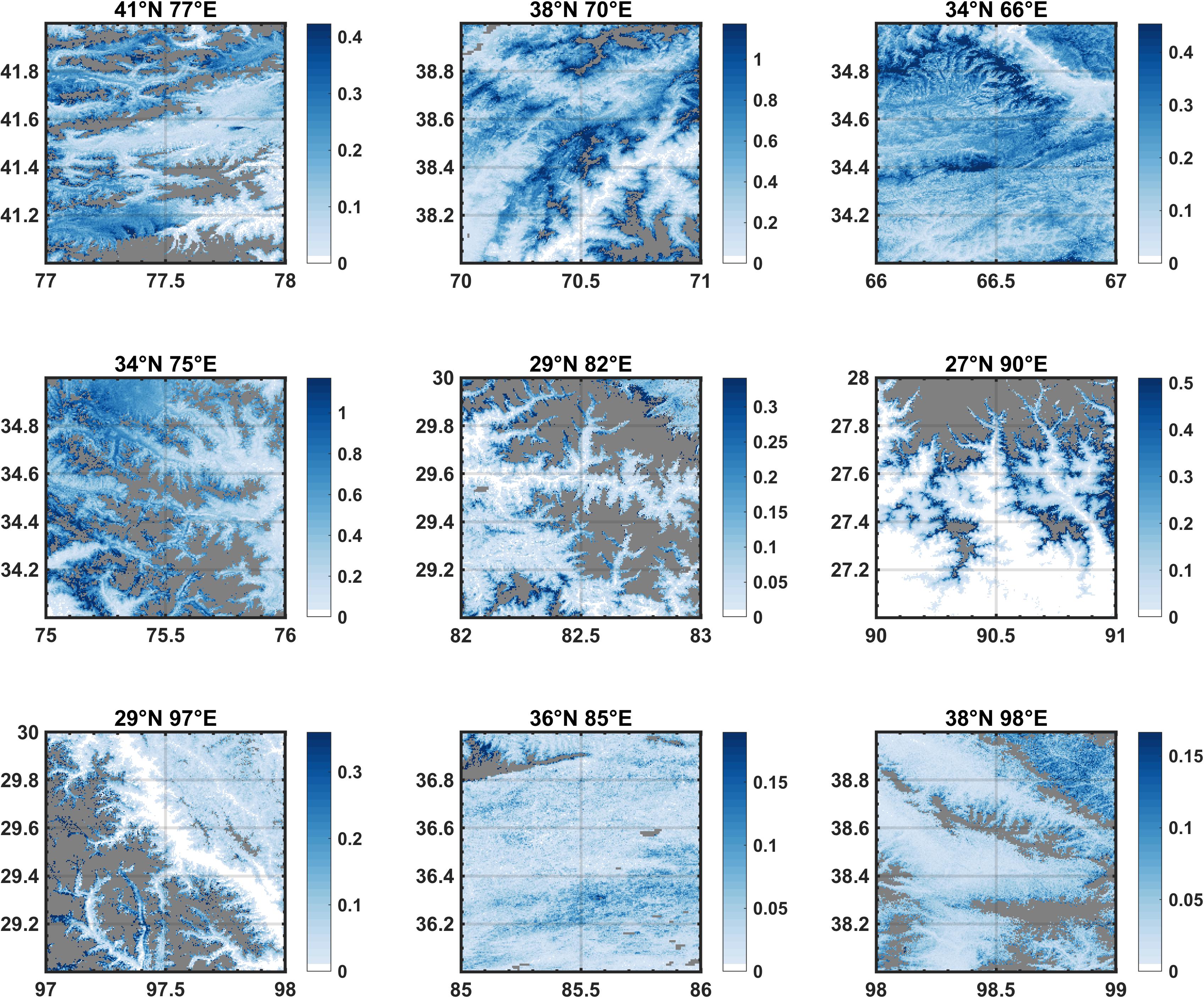
Figure 11. Maps of climatological (i.e., averaged over WYs 2000–2017) pixel-wise peak SWE (in meters) for the set of HMA test tiles. The gray pixels represent those masked out as pre-identified glaciers, likely glaciers (i.e., pixels with persistent carry-over SWE in more than 14 out of 18 years), or open water bodies. For reference, the tile DEMs are shown in Figure 1. The upper value used in the colorbars represent the 95th percentile of values in each map and not the maximum values.

Elevational Distribution of Posterior Peak SWE Climatology in HMA Test Tiles

The climatological maps can be used to aggregate SWE and illustrate how it varies with elevation across each tile. The SWE distribution is shown in Figure 12 in terms of both the average depth (SWE in meters) and integrated volume (SWE in km³) in each elevation band. Both are complementary in that the former illustrates how physical processes (e.g., orographic precipitation and snowfall vs. rainfall occurrence) may drive variations in SWE depth accumulation, while the latter merges that information with the hypsometry (i.e., area-elevation relationship) for each tile to get SWE volume storage. The SWE depth (Figure 12A) generally shows a strong gradient with respect to elevation. Tiles (27°N, 90°E) and (29°N, 97°E) show essentially no SWE at the lowest elevations, while the others have non-negligible SWE across the full range of elevations in the tiles. Tiles (34°N, 66°E), (41°N, 77°E) and (38°N, 98°E) show a relatively linear SWE lapse rate across the tile elevation range, while the other tiles show a non-linear relationship with an increasing lapse rate with elevation. The largest SWE depth values occur in the upper elevation bins in (27°N, 90°E) with over 1.5 m and (38°N, 70°E) with ∼1 m. Generally speaking, the relative tile area will decrease with increasing elevation, which is reflected in the SWE volume distribution (Figure 12B), where the peak volumes are generally stored at intermediate elevations. For reference, the cumulative fractional volume distribution and the median elevation within each tile are shown. Tiles (34°N, 66°E), (36°N, 85°E) exhibit distributions where the SWE volume storage is split approximately equally above and below the median tile elevation. Otherwise most of the tiles, including (34°N, 75°E), (41°N, 77°E), (29°N, 82°E), (29°N, 97°E), and (38°N, 98°E) have more than 50% of the SWE stored below the median elevation, while tiles (38°N, 70°E) and (27°N, 90°E) have more than 50% of the SWE stored above the median elevation. Tile (27°N, 90°E) stands out with ∼75% of its SWE volume stored above the median elevation.

FIGURE 12

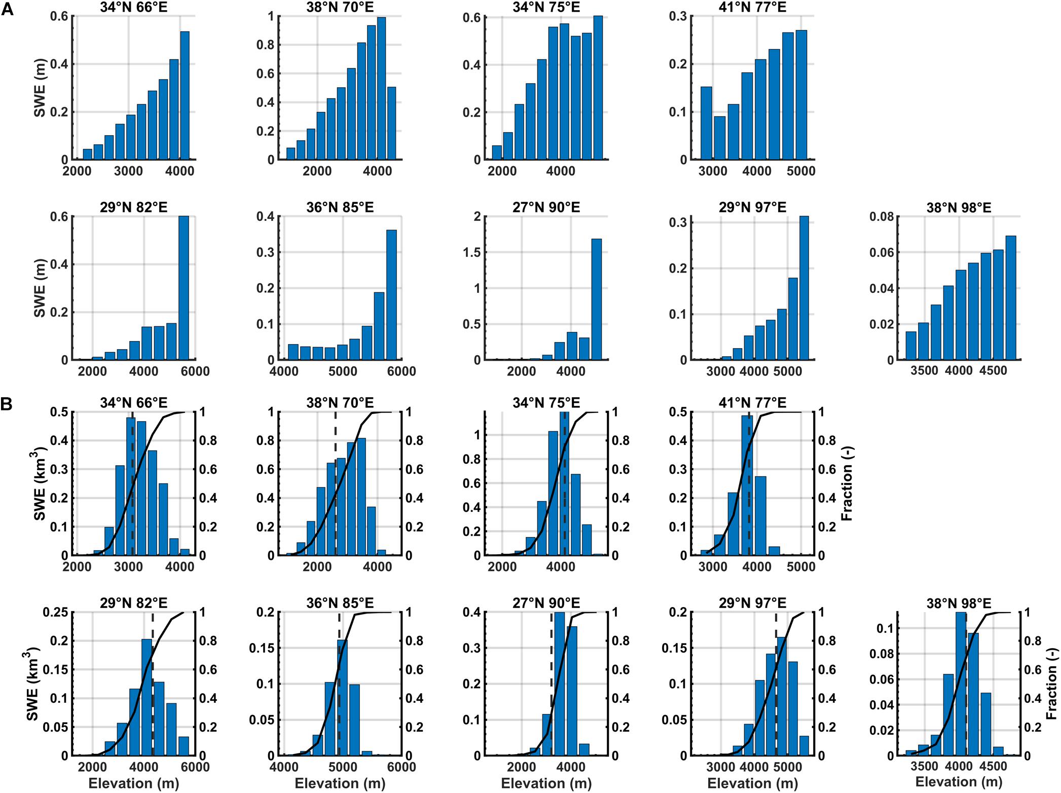
Figure 12. SWE distribution as a function of elevation for HMA test tiles expressed as: (A) bin-averaged SWE depth (in meters) and (B) bin-averaged SWE volume (in km³). For the SWE volume distributions, the cumulative distribution function (solid black line) showing the cumulative fraction of stored volume (right axis) and location of the median elevation (dark gray dashed line) is also shown.

Seasonal Cycle of Posterior SWE in HMA Test Tiles

To illustrate the seasonal nature of SWE storage we show the climatological seasonal cycle in tile-integrated SWE in each test tile along with the individual annual realizations over the 18 WYs examined (Figure 13). This is done by tile-averaging SWE for each day of the WY (to get annual time series) and then averaging across WYs to get the climatology. The seasonal cycle highlights some of the variations in snow drivers across the nine tiles. Of the tiles examined, the most canonical winter accumulation/spring melt examples are those in the western portion of the domain, i.e., (41°N, 77°E), (38°N, 70°E), (34°N, 75°E), and (34°N, 66°E), where there is a clear unimodal seasonal signature driven by precipitation in the winter and melt in the spring. Tiles (34°N, 75°E) and (38°N, 70°E) show the largest seasonal storage, with an average peak (interannual range) of ∼3.25 km³ (1.5–4.75 km³) and ∼3.25 km³ (1.75–5 km³), respectively, peaking around DOWY 175–200 (late-March to mid-April). Tiles (34°N, 66°E) and (38°N, 70°E) exhibit negligible carry-over seasonal SWE from 1 year to the next, while (41°N, 77°E) and (34°N, 75°E) have carry-over in some years. The remaining tiles (when moving east), show a much more mixed seasonal behavior with monsoonal influence evident in the SWE annual cycle. For example, most of these tiles have precipitation in the spring/summer season (i.e., after DOWY 200) extending into the fall (i.e., before DOWY 50) with very limited precipitation in between. This results in a seasonal shift where SWE can carry-over from one WY to the next and/or have multiple local maxima throughout the year. Tiles (27°N, 90°E), (29°N, 97°E), and (38°N, 98°E) appears to be the most monsoon-driven, with either peak SWE occurring later in the WY and/or common carry-over from spring to fall as a result, in part, of non-winter snowfall. The reduced ratio of winter to non-winter precipitation explains why SWE is limited to the highest elevations in these tiles (as shown in Figure 12), where air temperatures are cold enough in summer to allow for snow accumulation. The other tiles generally show a mix of winter/summer precipitation. Tile (38°N, 98°E) show two peaks, one driven by early fall precipitation (i.e., before DOWY 50) and a larger peak around DOWY 220.

FIGURE 13

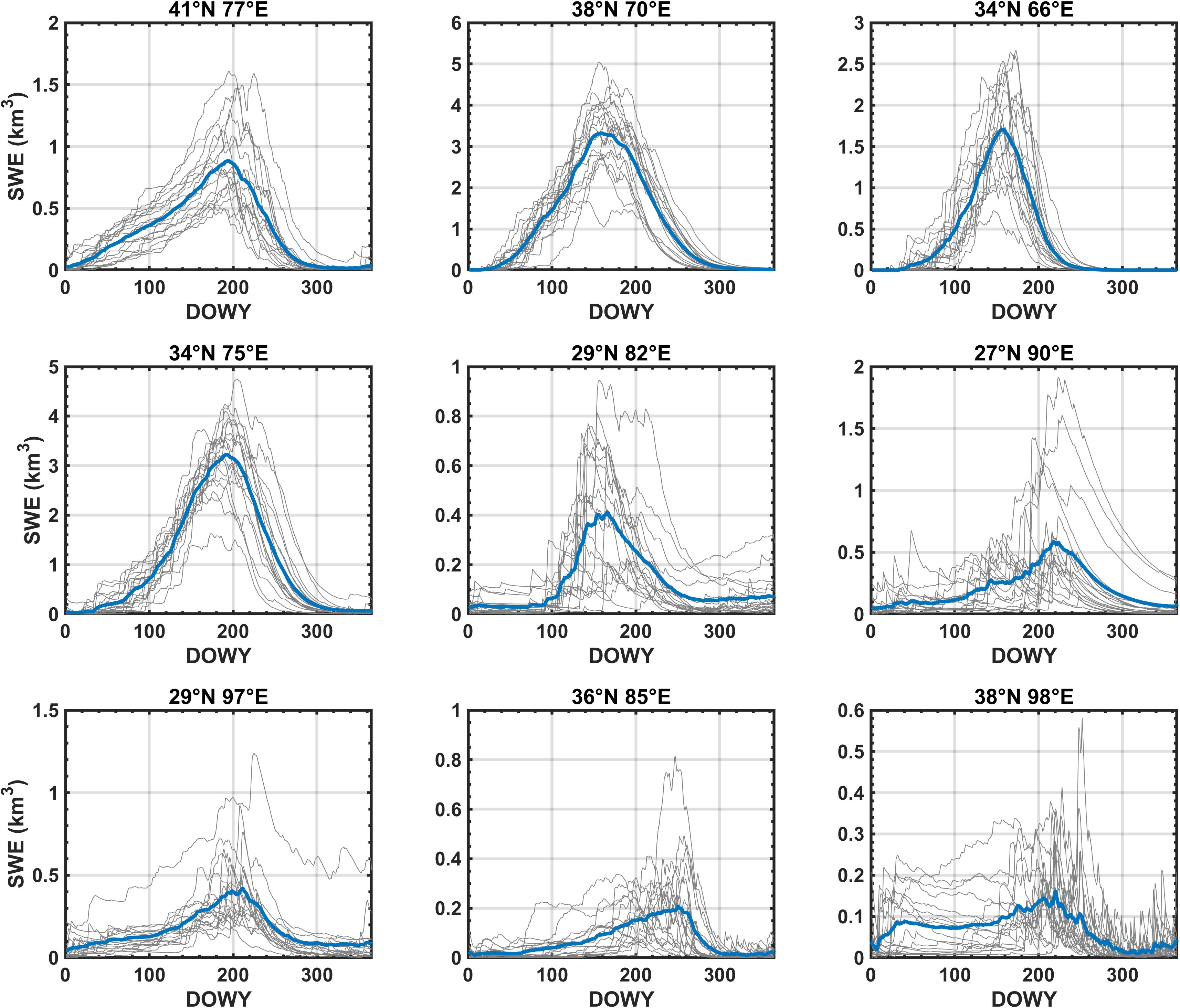
Figure 13. Tile-averaged seasonal cycle in SWE volume (km³) for HMA test tiles. The 18-year climatology is shown with the thick blue line. Individual years are shown with thin gray lines for reference.

Summary and Conclusion

The snow reanalysis framework presented herein is designed to provide a methodology for estimating seasonal snow storage and its dynamics in global midlatitude mountain regimes where in situ observations are severely lacking. The method leverages existing readily available global datasets for forcing a snow model and Landsat- and MODIS-derived (MODSCAG) fSCA retrievals to update the prior model estimates in order to derive posterior estimates using a Bayesian framework. The DA framework not only jointly uses Landsat and MODSCAG fSCA data, but accounts for MODIS viewing -geometry effects on the fSCA retrievals through: (i) accounting for expected variations in measurement error covariance and (ii) a screening and CDF-matching technique that leverages the high-resolution (near-nadir) sampling of Landsat to transform the MODIS measurements to a consistent basis before assimilation. The method was verified through comparison with the Airborne Snow Observatory (ASO) SWE estimates over the Tuolumne River watershed in California. The posterior SWE estimates were shown to be much more consistent with the independent ASO estimates across the three WYs examined. Tests over Tuolumne showed that, where a large number of Landsat measurements exist (i.e., in areas of overlapping Landsat tiles and multiple sensors), the Landsat-only case performance is best, attributable primarily to the higher spatial resolution of the raw Landsat data, but that with fewer Landsat measurements (i.e., in areas with only single Landsat tile coverage or significant cloud cover), the additional MODIS-based measurements can have a positive impact. Illustrative results were presented for nine HMA test tiles to illustrate how the method can provide posterior estimates of the space-time climatology in SWE storage in areas where in situ data does not generally exist. Ongoing work is being conducted to use the method outlined herein to generate an HMA-wide reanalysis dataset that will provide an opportunity for a more thorough characterization of seasonal snow storage and dynamics over the joint Landsat-MODIS era as well as putting it in the context of other studies that have characterized seasonal snow in HMA. Additional future avenues of research could include a detailed exploration of different forcing datasets (i.e., MERRA-2, ERA5, GLDAS, etc.) and their implications, and the usage or addition of other fSCA products (i.e., from VIIRS) using the framework developed herein.

Data Availability Statement

The datasets generated for this study are available on request to the corresponding author.

Author Contributions

SM conceived of and supervised the project, provided guidance, led the method verification over the Sierra Nevada domain, and wrote the manuscript. YL led the implementation of the method over the HMA domain tiles and led that analysis. EB helped in the development of the methods and contributed to an early draft of the manuscript.

Funding

This work was funded by the NASA High Mountain Asia Program Grant #NNX16AQ63G.

Conflict of Interest

The authors declare that the research was conducted in the absence of any commercial or financial relationships that could be construed as a potential conflict of interest.

Acknowledgments

We would like to thank those responsible for the creation of the datasets used in this study as well as members of the NASA High Mountain Asia Team (HiMAT) who have helped shape the overall direction of the work. G. Cortes is acknowledged for pre-processing some of the input data used in the snow reanalysis over the HMA domain. The two reviewers are acknowledged for their helpful comments which greatly improved the manuscript.

Footnotes

1. ^ https://www.usgs.gov/land-resources/nli/landsat/data-tools
2. ^ https://snow.jpl.nasa.gov/portal/data/
3. ^ https://nsidc.org/data/aso/data-summaries

References

Adam, J. C., and Lettenmaier, D. P. (2003). Adjustment of global gridded precipitation for systematic bias. J. Geophys. Res. 108, 4257–4272.

Google Scholar

Andreadis, K. M., and Lettenmaier, D. P. (2006). Assimilating remotely sensed snow observations into a macroscale hydrology model. Adv. Water Resour. 29, 872–886. doi: 10.1016/j.advwatres.2005.08.004

CrossRef Full Text | Google Scholar

Arsenault, K. R., Houser, P. R., De Lannoy, G. J. M., and Dirmeyer, P. A. (2013). Impacts of snow cover fraction data assimilation on modeled energy and moisture budgets. J. Geophys. Res. 118, 7489–7504. doi: 10.1002/jgrd.50542

CrossRef Full Text | Google Scholar

Baldo, E., and Margulis, S. (2018). Assessment of a multi-resolution snow reanalysis framework: a multi-decadal reanalysis case over the Upper Yampa River Basin. Colorado 22, 3575–3587. doi: 10.5194/hess-22-3575-2018

CrossRef Full Text | Google Scholar

Baldo, E., and Margulis, S. A. (2017). Implementation of a physiographic complexity-based multiresolution snow modeling scheme. Water Resour. Res. 53, 3680–3694. doi: 10.1002/2016wr020021

CrossRef Full Text | Google Scholar

Barnett, T. P., Adam, J. C., and Lettenmaier, D. P. (2005). Potential impacts of a warming climate on water availability in snow-dominated regions. Nature 438, 303–309. doi: 10.1038/nature04141

PubMed Abstract | CrossRef Full Text | Google Scholar

Chang, A., Foster, J., and Hall, D. (1987). Nimbus-7 SMMR derived global snow cover parameters. Ann. Glaciol. 9, 39–44. doi: 10.1017/s0260305500200736

CrossRef Full Text | Google Scholar

Clark, M. P., Slater, A. G., Barrett, A. P., Hay, L. E., McCabe, G. J., Rajagopalan, B., et al. (2006). Assimilation of snow covered area information into hydrologic and land-surface models. Adv. Water Resour. 29, 1209–1221. doi: 10.1016/j.advwatres.2005.10.001

CrossRef Full Text | Google Scholar

Cortes, G., Girotto, M., and Margulis, S. A. (2014). Analysis of sub-pixel snow and ice extent over the extratropical andes using spectral unmixing of historical landsat imagery. Remote Sens. Environ. 141, 64–78. doi: 10.1016/j.rse.2013.10.023

CrossRef Full Text | Google Scholar

Cortes, G., and Margulis, S. (2017). Impacts of el nino and la ninÞa on interannual snow accumulation in the andes: results from a high-resolution 31 year reanalysis. Geophys. Res. Lett. 44, 6859–6867. doi: 10.1002/2017gl073826

CrossRef Full Text | Google Scholar

Cosgrove, B. A., Lohmann, D., Mitchell, K. E., Houser, P. R., Wood, E. F., Schaake, J. C., et al. (2003). Real-time and retrospective forcing in the north american land data assimilation system (nldas) project. J. Geophys. Res. 108:8842.

Google Scholar

De Lannoy, G. J. M., Reichle, R. H., Arsenault, K. R., Houser, P. R., Kumar, S., Verhoest, N. E. C., et al. (2012). Multiscale assimilation of advanced microwave scanning radiometer snow water equivalent and moderate resolution imaging spectroradiometer snow cover fraction observations in northern colorado. Water Resour. Res. 48:W01522.

Google Scholar

De Lannoy, G. J. M., Reichle, R. H., Houser, P. R., Arsenault, K. R., Verhoest, N. E. C., and Pauwels, V. R. N. (2010). Satellite-scale snow water equivalent assimilation into a high-resolution land surface model. J. Hydrometeorol. 11, 352–369. doi: 10.1175/2009jhm1192.1

CrossRef Full Text | Google Scholar

Dozier, J., Bair, E. H., and Davis, R. E. (2016). Estimating the spatial distribution of snow water equivalent in the world’s mountains. WIREs Water 3, 461–474. doi: 10.1002/wat2.1140

CrossRef Full Text | Google Scholar

Dozier, J., Painter, T. H., Rittger, K., and Frew, J. E. (2008). Time–space continuity of daily maps of fractional snow cover and albedo from modis. Adv. Water Resour. 31, 1515–1526. doi: 10.1016/j.advwatres.2008.08.011

CrossRef Full Text | Google Scholar

Durand, M., Kim, E., and Margulis, S. (2009). Radiance assimilation shows promise for snowpack characterization. Geophys. Res. Lett. 36, L02503. doi: 10.1029/2008GL035214

CrossRef Full Text | Google Scholar

Durand, M., and Margulis, S. (2007). Correcting first-order errors in snow water equivalent estimation using a multi-frequency, multi-scale data assimilation scheme. J. Geophys. Res. 112, D13121.1–D13121.15. doi: 10.1029/2006JD008067

CrossRef Full Text | Google Scholar

Farr, T. G., Rosen, P. A., Caro, E., Crippen, R., Duren, R., Hensley, S., et al. (2007). The shuttle radar topography mission. Rev. Geophys. 45:RG2004.

Google Scholar

Frei, A., Tedesco, M., Lee, S., Foster, J., Hall, D. K., Kelly, R., et al. (2012). A review of global satellite-derived snow products. Adv. Space Res. 50, 1007–1029. doi: 10.1016/j.asr.2011.12.021

CrossRef Full Text | Google Scholar

Gelaro, R., McCarty, W., Sua ìrez, M. J., Todling, R., Molod, A., Takacs, L., et al. (2017). The modern- era retrospective analysis for research and applications, version 2 (merra-2). J. Clim. 30, 5419–5454. doi: 10.1175/jcli-d-16-0758.1

CrossRef Full Text | Google Scholar

Girotto, M., Cortes, G., Margulis, S. A., and Durand, M. (2014a). Examining spatial and temporal variability in snow water equivalent using a 27 year reanalysis: Kern river watershed, sierra nevada. Water Resour. Res. 50, 6713–6734. doi: 10.1002/2014wr015346

CrossRef Full Text | Google Scholar

Girotto, M., Margulis, S. A., and Durand, M. (2014b). Probabilistic swe reanalysis as a generalization of deterministic swe reconstruction techniques. Hydrol. Process. 28, 3875–3895. doi: 10.1002/hyp.9887

CrossRef Full Text | Google Scholar

GLIMS and NSIDC, (2018). Global Land Ice Measurements from Space glacier database. Boulder, CO: National Snow and Ice Data Center.

Google Scholar

Global Modeling and Assimilation Office [GMAO], (2015a). MERRA-2 tavg1_2d_flx_Nx: 2d,1-Hourly, Time-Averaged, Single-Level, Assimilation, Surface Flux Diagnostics V5.12.4. Greenbelt, MD: Goddard Earth Sciences Data and Information Services Center (GES DISC).

Google Scholar

Global Modeling and Assimilation Office [GMAO], (2015b). MERRA-2 tavg1_2d_rad_Nx: 2d,1-Hourly, Time-Averaged, Single-Level, Assimilation, Radiation Diagnostics V5.12.4. Greenbelt, MD: Goddard Earth Sciences Data and Information Services Center (GES DISC).

Google Scholar

Global Modeling and Assimilation Office [GMAO], (2015c). MERRA-2 tavg1_2d_slv_Nx: 2d,1-Hourly, Time-Averaged, Single-Level, Assimilation, Single-Level Diagnostics V5.12.4. Greenbelt, MD: Goddard Earth Sciences Data and Information Services Center (GES DISC).

Google Scholar

Hansen, M. C., Defries, R. S., Townshend, J. R. G., and Sohlberg, R. (2000). Global land cover classification at 1 km spatial resolution using a classification tree approach. Int. J. Remote Sens. 21, 1331–1364. doi: 10.1080/014311600210209

CrossRef Full Text | Google Scholar

Huning, L. S., and Margulis, S. A. (2017). Climatology of seasonal snowfall accumulation across the Sierra Nevada (USA): accumulation rates, distributions, and variability. Water Resour. Res. 53, 6033–6049. doi: 10.1002/2017WR020915

CrossRef Full Text | Google Scholar

Kovalskyy, V., and Roy, D. (2013). The global availability of Landsat 5 TM and Landsat 7 ETM+ land surface observations and implications for global 30m landsat data product generation. Remote Sens. Environ. 130(Suppl. C), 280–293. doi: 10.1016/j.rse.2012.12.003

CrossRef Full Text | Google Scholar

Kumar, S. V., Peters-Lidard, C. D., Arsenault, K. R., Getirana, A., Mocko, D., and Liu, Y. (2015a). Quantifying the added value of snow cover area observations in passive microwave snow depth data assimilation. J. Hydrometeorol. 16, 1736–1741. doi: 10.1175/jhm-d-15-0021.1

CrossRef Full Text | Google Scholar

Kumar, S. V., Peters-Lidard, C. D., Santanello, J. A., Reichle, R. H., Draper, C. S., Koster, R. D., et al. (2015b). Evaluating the utility of satellite soil moisture retrievals over irrigated areas and the ability of land data assimilation methods to correct for unmodeled processes. Hydrol. Earth Syst. Sci. 19, 4463–4478. doi: 10.5194/hess-19-4463-2015

CrossRef Full Text | Google Scholar

Kwon, Y., Yang, Z. L., Hoar, T. J., and Toure, A. M. (2017). Improving the radiance assimilation performance in estimating snow water storage across snow and land-cover types in North America. J. Hydrometeorol. 18, 651–668. doi: 10.1175/jhm-d-16-0102.1

CrossRef Full Text | Google Scholar

Lettenmaier, D. P., Alsdorf, D., Dozier, J., Huffman, G. J., Pan, M., and Wood, E. F. (2015). Inroads of remote sensing into hydrologic science during the WRR era. Water Resour. Res. 51, 7309–7342. doi: 10.1002/2015WR017616

CrossRef Full Text | Google Scholar

Li, D., Durand, M., and Margulis, S. A. (2017). Estimating snow water equivalent in a Sierra Nevada watershed via spaceborne radiance data assimilation. Water Resour. Res. 53, 647–671. doi: 10.1002/2016WR018878

CrossRef Full Text | Google Scholar

Liston, G. E. (2004). Representing subgrid snow cover heterogeneities in regional and global models. J. Clim. 17, 1381–1397. doi: 10.1175/1520-0442(2004)017<1381:rsschi>2.0.co;2

CrossRef Full Text | Google Scholar

Liston, G. E., and Elder, K. (2006). A meteorological distribution system for high-resolution terrestrial modeling (micromet). J. Hydrometeorol. 7, 217–234. doi: 10.1175/jhm486.1

CrossRef Full Text | Google Scholar

Liu, Y., Parinussa, R. M., Dorigo, W. A., De Jeu, R. A. M., Wagner, W., van Dijk, A. I. J. M., et al. (2011). Developing an improved soil moisture dataset by blending passive and active microwave satellite-based retrievals. Hydrol. Earth Syst. Sci. 15, 425–436. doi: 10.5194/hess-15-425-2011

CrossRef Full Text | Google Scholar

Liu, Y., Peters-Lidard, C. D., Kumar, S., Foster, J. L., Shaw, M., Tian, Y., et al. (2013). Assimilating satellite-based snow depth and snow cover products for improving snow predictions in alaska. Adv. Water Resour. 54(Suppl. C), 208–227. doi: 10.1016/j.advwatres.2013.02.005

CrossRef Full Text | Google Scholar

Mankin, J. S., Viviroli, D., Singh, D., Hoekstra, A. Y., and Diffenbaugh, N. S. (2015). The potential for snow to supply human water demand in the present and future. Environ. Res. Lett. 10:114016. doi: 10.1088/1748-9326/10/11/114016

CrossRef Full Text | Google Scholar

Margulis, S. A., Cortes, G., Girotto, M., and Durand, M. (2016a). A Landsat-era sierra nevada snow reanalysis (1985–2015). J. Hydrometeorol. 17, 1203–1221. doi: 10.1175/jhm-d-15-0177.1

CrossRef Full Text | Google Scholar

Margulis, S., Cortes, G., Girotto, M., Huning, L., Li, D., and Durand, M. (2016b). Characterizing the extreme 2015 snowpack deficit in the Sierra Nevada (USA) and implications for recovery. Geophys. Res. Lett. 43, 6341–6349. doi: 10.1002/2016GL068520

CrossRef Full Text | Google Scholar

Margulis, S. A., Girotto, M., Cortes, G., and Durand, M. (2015). A particle batch smoother approach to snow water equivalent estimation. J. Hydrometeorol. 16, 1752–1772. doi: 10.1175/jhm-d-14-0177.1

CrossRef Full Text | Google Scholar

NASA, (2001). ASTER DEM Product. Sioux Falls, SD: NASA.

Google Scholar

Painter, T. H., Berisford, D. F., Boardman, J. W., Bormann, K. J., Deems, J. S., Gehrke, F., et al. (2016). The airborne snow observatory: fusion of scanning lidar, imaging spectrometer, and physically-based modeling for mapping snow water equivalent and snow albedo. Remote Sens. Environ. 184, 139–152. doi: 10.1016/j.rse.2016.06.018

CrossRef Full Text | Google Scholar

Painter, T. H., Rittger, K., McKenzie, C., Slaughter, P., Davis, R. E., and Dozier, J. (2009). Retrieval of subpixel snow covered area, grain size, and albedo from modis. Remote Sens. Environ. 113, 868–879. doi: 10.1016/j.rse.2009.01.001

CrossRef Full Text | Google Scholar

Pierce, D. W., Cayan, D. R., and Thrasher, B. L. (2014). Statistical downscaling using localized constructed analogs (LOCA). J. Hydrometeorol. 15:2558. doi: 10.1175/JFM-D-14-0082.1

CrossRef Full Text | Google Scholar

Reichle, R. H., and Koster, R. D. (2004). Bias reduction in short records of satellite soil moisture. Geophys. Res. Lett. 31:L19501.

Google Scholar

Reichle, R. H., Koster, R. D., Liu, P., Mahanama, S. P. P., Njoku, E. G., and Owe, M. (2007). Comparison and assimilation of global soil moisture retrievals from the advanced microwave scanning radiometer for the earth observing system (AMSR-E) and the scanning multichannel microwave radiometer (SMMR). J. Geophys. Res. 112:D09108. doi: 10.1029/2006JD008033

CrossRef Full Text | Google Scholar

Rhoades, A. M., Ullrich, P. A., Zarzycki, C. M., Johansen, H., Margulis, S. A., Morrison, H., et al. (2018). Sensitivity of mountain hydroclimate simulations in variable-resolution CESM to microphysics and horizontal resolution. J. Adv. Model. Earth Syst. 10, 1357–1380. doi: 10.1029/2018MS001326

CrossRef Full Text | Google Scholar

Rohrer, M., Salzmann, N., Stoffel, M., and Kulkarni, A. (2013). Missing (in-situ) snow cover data hampers climate change and runoff studies in the greater himalayas. Sci. Total Environ. 46, S60–S70. doi: 10.1016/j.scitotenv.2013.09.056

PubMed Abstract | CrossRef Full Text | Google Scholar

Serreze, M. C., Clark, M. P., Armstrong, R. L., McGinnis, D. A., and Pulwarty, R. S. (1999). Characteristics of the western united states snowpack from snowpack telemetry (snotel) data. Water Resour. Res. 35, 2145–2160. doi: 10.1029/1999wr900090

CrossRef Full Text | Google Scholar

Sexton, J. O., Song, X.-P., Feng, M., Noojipady, P., Anand, A., Huang, C., et al. (2013). Global, 30-m resolution continuous fields of tree cover: Landsat-based rescaling of modis vegetation continuous fields with lidar-based estimates of error. Int. J. Digit. Earth 6, 427–448. doi: 10.1080/17538947.2013.786146

CrossRef Full Text | Google Scholar

Su, H., Yang, Z.-L., Niu, G.-Y., and Dickinson, R. E. (2008). Enhancing the estimation of continental-scale snow water equivalent by assimilating modis snow cover with the ensemble kalman filter. J. Geophys. Res. 113:D08120.

Google Scholar

Sun, S., and Xue, Y. (2001). Implementing a new snow scheme in simplified simple biosphere model. Adv. Atmos. Sci. 18, 335–354. doi: 10.1007/bf02919314

CrossRef Full Text | Google Scholar

Tedesco, M., Reichle, R., Low, A., Markus, T., and Foster, J. (2010). Dynamic approaches for snow depth retrieval from spaceborne microwave brightness temperature. IEEE Trans. Geosci. Remote Sens. 48, 1955–1967. doi: 10.1109/tgrs.2009.2036910

CrossRef Full Text | Google Scholar

Tsang, L., Pan, J., Liang, D., Li, Z., Cline, D. W., and Tan, Y. (2007). Modeling active microwave remote sensing of snow using dense media radiative transfer (DMRT) theory with multiple-scattering effects. IEEE Trans. Geosci. Remote Sens. 45, 990–1004. doi: 10.1109/tgrs.2006.888854

CrossRef Full Text | Google Scholar

Ulaby, F. T., and Stiles, W. H. (1980). The active and passive microwave response to snow parameters: 2. Water equivalent of dry snow. J. Geophys. Res. 85, 1045–1049.

Google Scholar

Wrzesien, M. L., Durand, M. T., Pavelsky, T. M., Kapnick, S., Zhang, Y., Guo, J., et al. (2018). A new estimate of north american mountain snow accumulation from regional climate model simulations. Geophys. Res. Lett. 45, 1423–1432. doi: 10.1002/2017gl076664

CrossRef Full Text | Google Scholar

Wulder, M. A., White, J. C., Loveland, T. R., Woodcock, C. E., Belward, A. S., Cohen, W. B., et al. (2016). The global Landsat archive: status, consolidation, and direction. Remote Sens. Environ. 185, 271–283. doi: 10.1016/j.rse.2015.11.032

CrossRef Full Text | Google Scholar

Xia, Y., Mitchell, K., Ek, M., Sheffield, J., Cosgrove, B., Wood, E., et al. (2012). Continental-scale water and energy flux analysis and validation for the north american land data assimilation system project phase 2 (nldas-2): 1. Intercomparison and application of model products. J. Geophys. Res. 117:D03109. doi: 10.1029/2011JD016048

CrossRef Full Text | Google Scholar

Xue, Y., Sun, S., Kahan, D. S., and Jiao, Y. (2003). Impact of parameterizations in snow physics and interface processes on the simulation of snow cover and runoff at several cold region sites. J. Geophys. Res. 108:8859. doi: 10.1029/2002JD003174

CrossRef Full Text | Google Scholar