Well-Posed Geoscientific Visualization Through Interactive Color Mapping

Introduction

Graphical representations in the form of static diagrams, plots, and charts form a fundamental part of the scientific toolset. Scientific visualization aims to reveal and explore relationships in data and assist in the development of robust inference, posing two initial questions of data: “Is what we see really there?” and “Is there something there we cannot see?” The first question encapsulates the interplay between scientific curiosity and apophenia—“the innate human ability to see pattern in noise” (Wickham et al., 2010; Cook, 2017). The second question exposes the concept of “missed discovery,” where the analyst is unaware that unperceived structures await discovery (Buja et al., 2009).

Important challenges are thus posed to software designed for visual analytics (Keim et al., 2006) and data-based graphical inference (Cook et al., 2016). Interactive computer-based visualizations can expand the explanatory and exploratory capabilities of scientific software. A significant body of research in visualization, interactivity, analysis and design (e.g., Tukey, 1990; Wilkinson, 2005; Ward et al., 2010; Ware, 2013; Munzner, 2014) provides the foundations for visualization practice.

Well-posed visualizations clearly elicit features of underlying data values, maintaining an overt awareness of the risks of representational ambiguity and error (Rougier et al., 2014). Given the constraints of a human-computer visualization system (Haber and McNabb, 1990; Hansen and Johnson, 2005), they can reveal structures and patterns that may be elusive to other, e.g., statistical, approaches (Tukey, 1977, 1990; Tufte, 1990). The informational capacity of static images can be extended by incorporating elements of interactivity (Ward et al., 2010).

Interactivity enables the exploration of the design-space for visualization (Schulz et al., 2013), including constraints for visual encoding and interaction idioms (Munzner, 2014), creating a feedback loop between user and visualization system. Representations may be examined in detail, forming an important part of the analytical and inferential processes (Keim, 2001; Keim et al., 2006) that actively facilitate conceptual model building and analyses (Keim et al., 2010; Ward et al., 2010; Harold et al., 2016).

Background and Related Work

The Interactive Visualization Process

A model of the interactive visualization process (Figure 1) proposes three principal components: “Data,” “Visualization,” and “User.” Data (D) is transformed by a specification (S) into a visualization (V). The Image (I) is processed by the perception and cognition of the user (P) to produce knowledge (K), iterated via a time-variant perceptual/cognitive loop (dK/dt), in concert with interactive exploration (IE). Time-variant specification changes (dS/dt) in turn affect V. More explicitly, D undergoes some pre-processing and transformation into an interrogable structure before it is visualized. S includes interactive steps including filtering, mapping, and rendering, affecting the appearance of the visualization. This is pertinent to mapping variables to color, given the interplay between machine models of color spaces (S) and perceptual faculties of users (P) in their context of observation. P implicitly incorporates the context in which a visualization is observed. This includes factors such as ambient illumination conditions and changes in lighting (e.g., shadows and light in a room or daylight through a window). These are all normal criteria for screen and print reproduction quality control in professional digital publishing, and merit greater consideration for well-posed scientific visualization.

FIGURE 1

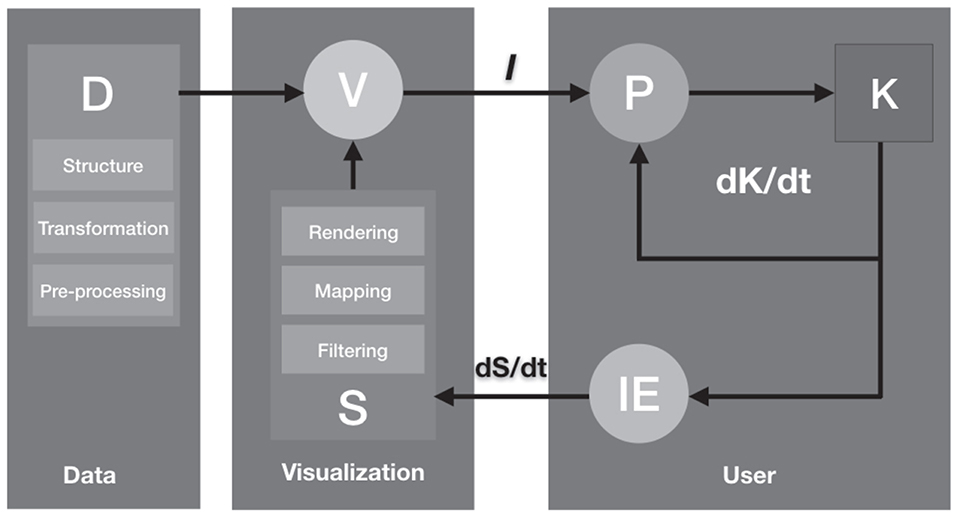
Figure 1. Model of Visualization (after Van Wijk, 2005 and Liu et al., 2014). This figure shows a schematic model of the visualization process, incorporating human-computer interaction.

Colormaps and Color Scales in Scientific Visualization

Colormaps and color-scales are standard features in interactive scientific visualization software aiming to convey a wide variety of information types: e.g., continuous values, categories and many others (Rheingans, 1992, 2000; Munzner, 2014; Mittelstädt and Keim, 2015; Zhou and Hansen, 2016). Colorization of data can be driven parametrically, e.g., using algorithmic functions (Eisemann et al., 2011), by human aesthetic decisions (Healey and Enns, 2012) or by pre-existing convention and experience (Bertin, 1983; MacEachren et al., 2012). The widely-used rainbow (“Jet”) or spectrum-approximation colormap, whilst having specific productive use-cases, is well-known for introducing problems of perceptual non-linearity, hue-ordering ambiguity and loss of visual discrimination for fine detail (Rogowitz and Treish, 1998; Eddins, 2014; Hawkins, 2015; Stauffer et al., 2015). Research into optimal colormap design for science has an extensive literature (Silva et al., 2011; Kovesi, 2015; Moreland, 2016; Ware et al., 2018), including optimization for color vision deficiencies (Light and Bartlein, 2004). Addressing the need for consistent terminology, Bujack et al. (2018) propose a nomenclature with unambiguous mathematical definitions, characteristics that are quantifiable via their on-line tool (Bujack et al., 2018).

Colormaps that maximize color difference such as Viridis, Magma, Parula and others are now becoming default schemes in widely-used scientific software (Smith et al., 2015). Ware et al. (2018) and Kovesi (2015) provide thorough analysis of a range of colormaps for different visualization tasks. Crameri (2018a,b) provides extensive discussion of colormaps for geoscientific visualization, as well as software and colormap resources for widely used programs such as GMT, Matlab, QGIS and others.

Human Color Perception

Human color vision is a complex, adaptive system extensively studied by vision researchers (Wyszecki and Stiles, 1982; Gordon, 2004; Stockman and Brainard, 2015). Estimates of the number of discernible colors perceivable by an average human vary widely (Masaoka et al., 2013). The non-uniform nature of human color perception has been well-established by techniques in advanced colorimetry (Fairchild, 2013).

RGB, HSL, HSV Color

A simple computable model for linear RGB color calculates and stores color values as 8-bit values of the three primaries Red, Green, and Blue (RGB), following an additive color-mixing model capable of generating (2⁸)³ colors: 16.7 million colors or “24-bit color” (Poynton, 2012). Whilst computationally simple, RGB color mixing is regarded as non-intuitive for end-users (Meier et al., 2004; Zeileis and Hornik, 2006). Tractable transformations of RGB, such as HSL and HSV (Smith, 1978), are simple geometric reformulations of this schematic color model, rather than perception-based ones (Robertson, 1988), and inadequately represent human color perception (Poynton, 2006; Fairchild, 2013). Despite their ease-of-use and ubiquity in computer interfaces, they are discontinuous and not perceptually uniform. They also present problems in accurately representing color and lightness relationships (Light and Bartlein, 2004; Silva et al., 2011; Kovesi, 2015; Moreland, 2016; Ware et al., 2018). Most importantly for data visualization, there is no meaningful metric for representing color difference in RGB, HSL, or HSV color spaces that match human perception of color differences (Robertson, 1988).

CIE Color

The CIE system (CIE, 2004), an international standard for color specification and communication, provides a series of color models that mathematically represent human color perception and color appearance. The CIEXYZ 1931 model is a perceptually measured color space with known values (CIE, 2004). This model represents all colors that are perceivable by an observer with average eyesight (Fairchild, 2013; Asano et al., 2016). The range of colors produced by the model is referred to as its gamut (Morovic and Luo, 2001). Commonly used color models such as RGB, HSV, HSL, and CMYK exhibit limited gamuts, producing a substantially smaller range of colors than humans are capable of perceiving. Because these models are relative, they require a photometrically defined reference white point, CIE D₅₀/D₆₅ (Poynton, 2006), in order for color values to be mapped from one space to another (Poynton, 1994). The standard RGB (sRGB) color space and gamma curve, using CIE defined chromaticities and D₆₅ whitepoint, has become the default color space for computer OS and internet color management systems (Anderson et al., 1996; IEC, 1999; Hoffmann, 2000). However, whilst “absolute,” sRGB color space is not a perceptual color space and has a significantly smaller gamut than that of CIEXYZ derivatives (Hoffmann, 2000, 2008). Mathematical regularizations of CIEXYZ have led to color models such as CIELAB and others, which closely approximate human color perception (Fairchild, 2013).

Uniform Color Space: CIELAB

Plotting CIE XYZ tristimulus values in Cartesian coordinates produce perceptually non-uniform color spaces (CIE, 2007). Uniform Color Spaces (UCS) are mathematical transformations of the CIE 1931 XYZ gamut that represent color in a perceptually even fashion, defined by the CIE as a color space in which equal metric distances approximately predict and represent equal perceived color differences (Luo et al., 2006; Bujack et al., 2018). As perception-based color models, they more accurately map the human visual gamut and mitigate color-matching and color-difference problems.

CIELAB and other UCS are commonly proposed for creating perceptually uniform color sequences in data visualization (Meyer and Greenberg, 1980; Kovesi, 2015; Ware et al., 2018), despite known limitations and deficiencies (Wyszecki and Stiles, 1982; Sharma and Rodriguez-Pardo, 2012; Fairchild, 2013; Zeyen et al., 2018). They form a set of absolute color spaces defined against reference whites or standard illuminants defined by the CIE (Tkalcic and Tasic, 2003; Foster, 2008; Fairchild, 2013). Due to relative ease of computability, CIELAB has become widely used for color specification and color difference measurement. It provides a complete numerical descriptor of color in a perceptually uniform rectangular coordinate system (Hunter Associates Laboratory Inc., 2018).

Color Difference

The CIELAB UCS color difference metric, ΔE, is calculated as follows (Lindbloom, 2017):

$E_{ab}^{*}=\sqrt{{\left(L_1-L_2\right)}^2+{\left(a_1-a_2\right)}^2+{\left(b_1-b_2\right)}^2}$

for 0 ≤ L ≤ 100, −128 ≤ a ≤ 127, −128 ≤ b ≤ 127 (signed 8-bit integer), where L = lightness, a = green (−a) to red (+a), b = blue (−b) to yellow (+b).

Color differences for RGB values are calculated via transposition into CIELAB coordinates within the sRGB gamut, following standard conversion formulae and standard illuminant values (RGB to XYZ, XYZ to CIELAB; Brainard, 2003; Lindbloom, 2013). This provides a dimensionless Euclidean metric for color difference that can be linearly applied to known data values and ranges during color-mapping. ΔE values of ~2.3 correspond to a just-noticeable-difference (JND) in color stimuli for an average untrained observer (Sharma and Trussell, 1997; Mokrzycki and Tatol, 2011), indicated in Table 1. Color opponency can be verified in CIELCh space, using Chroma (C) and Hue (h) values, calculated:

$\begin{array}{l}C=\sqrt{a^2+b^2}\\ h_{ab}=atan2(b,a)\end{array}$

where atan2 is the 2-argument arctangent function.

TABLE 1

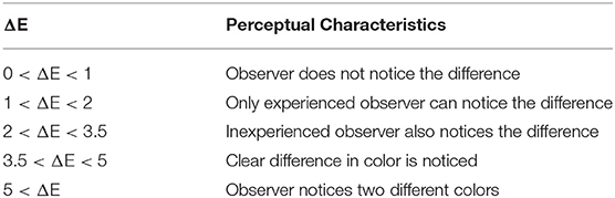
Table 1. ΔE perceptual characteristics (after Mokrzycki and Tatol, 2011).

3D Representations of Color

Most existing computer-based color-palette tools date back to paint programs from the 1980s (Meier et al., 2004). Standard 2D RGB/HSL/HSV color-selection interfaces do not clearly articulate the non-uniformity of human color perception and provide poorly defined feedback on color difference (Douglas and Kirkpatrick, 1999; Stauffer et al., 2015). 1D, 2D, and 3D representations of different color gamuts form an essential part of a user interface for color selection and application (Robertson, 1988; Zeileis and Hornik, 2006). Color gradients can be visualized as paths through representations of two or three-dimensional color spaces. Dimensionality is an imperative consideration in determining the type of path traversal that can be undertaken in a color space: 1D representations implicitly provide no path information, 2D representations address only co-planar colors, 3D representations provide maximal information about path extent, geometry and color relationships (Rheingans and Tebbs, 1990; Bergman et al., 1995). Path traversal is an important indicator for the location of perceptually isoluminant colors, indication of monotonicity (linear increase/decrease in chroma or lightness), quantization or stepping, orthogonality and other salient features (Ware, 1988; Bergman et al., 1995; Rogowitz and Goodman, 2012).

Data and Methods

Interactive Color-Mapping for Geoscience

Interactive color-mapping in an intuitive real-time, performant software application is an appealing proposition for geoscientific data visualization. Interactivity affords immediate visual feedback to the end-user, providing the opportunity to iterate through color palettes and associated colorization functions, exploring available color-spaces and their utility in eliciting features of underlying data. However, great care must be taken to ensure contiguity between data, color, and color-space geometries, including gradient path trajectories.

Although there are many applications that enable the construction of color gradients, few enable live interactive exploration of color spaces whilst being applied to data, concurrently providing visual feedback displaying the gradient path through color space. In this contribution we introduce Gradient Designer (GD), its companion applications and sample colormaps. This suite of tools is suitable not only for color-mapping, gradient design and data exploration, but extend live, real-time interactive visualization beyond the computer desktop to a range of visualization platforms, such as MR, VR, and Dome display systems (Milgram and Kishino, 1994; Morse and Bourke, 2012).

Implementation: Gradient Designer

Gradient Designer (GD) is an interactive gradient design and color-mapping software application aimed at the well-posed display of continuous spatial data, as frequently used in geoscience research. It is implemented on the MacOS platform (Morse, 2019).

GD features the following capabilities:

Data Handling:

• Local or remote datasets maybe be rapidly explored through an interactive interface that allows sequential overview of multiple layers through a 3D dataset, as well as zooming and panning to features of interest.

• Robust and clear relationship to known incoming data values and ranges enabled by UI.

• Export of high-resolution colorized images, as well as color gradients for import into other software in raster image format (.png), color palette table format (.cpt) and data interchange format (JSON).

Color Control:

• RGB gradients can be replicated and analyzed in CIELAB color space.

• Live color space visualization of gradient path traversal in CIELAB, RGB, HSL and HCL color spaces through four companion apps.

• Manipulation of linear RBG/sRGB (D₆₅) gamut colors in 3D CIELAB/RGB/HSL/HCL color spaces using simple HSL slider UI.

• Complex gradients may be designed that target specific values and ranges, including continuous-linear, stepped-linear, non-continuous and non-contiguous ranges.

Extended Functionality:

• Alpha channel control for downstream 3D compositing.

• Live video sharing of color gradient data to Syphon-compatible client applications for display (e.g., on immersive visualization systems).

Application Aims and Development Framework

Gradient Designer (GD) and its companion apps aim to provide an intuitive interface for a set of linear color-mapping tasks for continuous geoscience data. For our case study, data has been pre-processed into whole of globe equirectangular greyscale images stored as 8-bit RGB PNG files, with known data ranges (where 0–255 represent known minima and maxima, linearly mapped to the underlying data, including an alpha channel for lat/long region-of-interest delineation). This provides 256 greyscale values, which are adequate for the data under consideration.

The current version is programmed in the MacOS Quartz Composer VPL, using a mixture of pre-defined QC processing nodes as well as custom routines programmed in Objective-C, Javascript, OpenCL and OpenGL. It is compatible with MacOS 10.13.6 High Sierra and MacOS 10.14 Mojave (Morse, 2019). GD can share live video of the gradient display (Figure 2, panel 10) in real-time to external applications running a Syphon-compatible client (Butterworth et al., 2018; NewTek, 2019).

FIGURE 2

Figure 2. Gradient Designer User Interface. The 10 interface panels are listed in the figure and described in further detail in the text.

Gradient Designer User Interface

The user interface comprises two windows and standard MacOS menus, providing access to further color picker interfaces at OS-level. The application interface is designed around simple and familiar slider and button controls, and text field inputs. It uses a conventional mouse/keyboard combination.

Figure 2 illustrates the 10 main panels of the application: Panel 1—user instructions; Panel 2, a floating parameters window, provides access to file IO, global colorisation and composite operators, OS-level color pickers, output parameters and D₆₅ whitepoint XYZ reference values (IRO Group Ltd, 2019); Panel 3—interactive 3D Viewport; Panel 4—color picker controls—toggle on/off LAB Color Mixer input, GD or OS color picker controls; Panel 5—source image control and metadata; Panel 6—gradient display and design interface including data metric display; Panel 7—gradient control sliders for gradient layers; Panel 8—gradient and colorized data output previews; Panel 9—layer controls; Panel 10—output controls (Morse, 2019). Outputs include the ability to write out gradients as raster image formats (.png), color palette tables (.cpt; Wessel et al., 2013) and data interchange format (JSON), suitable for evaluation via colormeasures.org (Bujack et al., 2018).

Companion Applications

LAB Color Mixer (Figure 3) is a companion color-selection app for designing color gradients in CIELAB color space. LAB Color mixer displays RGB and CIELAB gradients in the same view, demonstrating the disparity between interpolation pathways in their respective color spaces. It displays CIELAB ΔE, as well as CIELCh Hue and Chroma values, for verification and color opponency. Companion visualization apps (Figure 3) GV_LAB, GV_RGB, GV_HSL, and GV_HCL run a continuous real-time image pixel evaluation, mapping incoming gradient color values to geometric positions in the visualized color spaces. The path through color space is drawn via OpenGL line segments in a looping refresh mode, providing visual feedback on the relationships between gradient termini, hinge-points and vectors in each color space. Dots along the path indicate the number of steps of the incoming gradient. This can be a compute-intensive process, so the detail density of the visualization can be reduced to speed up draw times, depending upon available GPU/CPU resources.

FIGURE 3

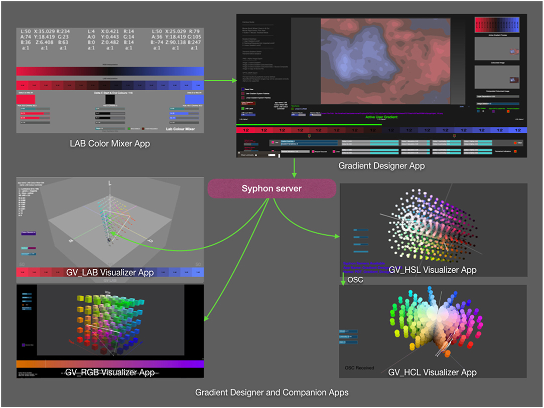
Figure 3. GD Color Space Visualization Companion Apps. This figure illustrates the workflow relationship between the LAB Color Mixer App, Gradient Designer and the four color space visualization apps, GV_LAB, GV_RGB, GV_HSL, and GV_HCL.

Example: CIELAB Divergent Gradient

Standard 2D color-picker GUIs impart limited information about the relationships between colors in a color space, requiring the user to infer characteristics that would be useful for scientific visualization, such as ΔE. LAB Color Mixer and GV_LAB apps address this gap.

LAB Color Mixer CIELAB gradients quantize in a binary fashion, enabling step ranges between 2 and 128. End termini are mapped first and interpolate toward the central value. For divergent gradients this ensures that gradient steps fall unambiguously either side of the central value. As quantization increases, we asymptotically approach the center value to the point of indistinguishability (ΔE <1), creating the appearance of a continuous gradient (JND <1). Colors in a three-point divergent gradient can be selected that maximize color difference, indicated by LAB and ΔE values. ΔE values displayed are rounded to the nearest integer. Unit-level quantization is sufficient for discriminability (see Table 1). The UI assists users in defining terminal colors that do not exceed the sRGB gamut by providing gamut warnings (where individual R, G, B values equal or exceed 0 or 255). LAB Color Mixer transmits the CIELAB-conformed color gradients as linear RGB image data via an addressable Syphon server to external client applications.

GV_LAB detects the Syphon server and draws the incoming linear RGB image data in CIELAB space, spatially transposed to the sRGB gamut representation (default: D₆₅, 2° Observer model). GV_LAB visualizes CIELAB color space three-dimensionally, displaying RGB gamut isoluminant colors on the AB plane, L on the vertical axis. This view can be rotated, zoomed and inspected. Path traversal lines between non-adjacent termini indicate where interpolated points may exceed the sRGB gamut. This provides instructive feedback for (a)symmetric gradient design, isoluminance and ΔE interpolation, enabling rapid identification of “problem” gradient regions as users explore the design space.

Case Study: Well-Posed Visualization of Seismic Tomography Depth Slices

As a test case for the visualization of a spatially variable 3D dataset in geoscience, we make use of a published seismic wavespeed model of the Earth's mantle beneath Australia, AuSREM (Kennett et al., 2013). In the following case study, we aim to display a 2D slice through the model in such a way as to:

• minimize the introduction of features that are visually salient, but not relevant to the interpretation.

• reveal distinctive features of the wavespeed in Earth's mantle. This is the most important intent of the visualization.

• manage, in a pragmatic way, the uncertainty in the numerical values.

• explore regions of interest in greater detail.

The Mantle Component of the Ausrem Seismic Tomography Model

The AuSREM model is a mature research product, aimed at capturing the distinctive features of the Earth's mantle for this continental area. It was constructed from several sources, primarily seismic surface wave tomography, supplemented by seismic body wave arrivals and regional tomography. The authors have minimized any artifacts of individual modeling procedures by combining 3D information from multiple sources. AuSREM is therefore a sensible choice of spatially variable dataset to use in the exploration of well-posed visualization approaches.

Data are supplied in the form of numerical seismic wavespeed values in 11 layers from 50 to 300 km, at 25 km intervals. Each layer is gridded at 0.5° intervals between −0.5 and −49.5° latitude, and 105.5 and 179.5° longitude. Wavespeed values are in the range 4.0–4.8 kms⁻¹ (Stål, 2019).

Uncertainty

For the purposes of this study, we assume the uncertainty in wavespeed to be constant throughout the model at ± 0.05 kms⁻¹, i.e., a given value of 4.20 kms⁻¹ could be between 4.15 and 4.25 but would not be as small as 4.14 nor as large as 4.26 kms⁻¹. We do not consider spatial uncertainty in this study, brought about by effects such as smearing, noted by Rawlinson et al. (2006). From a pragmatic perspective therefore, for a value at a given point, the uncertainty is the maximum departure from the given value within which an experienced analyst would expect the actual value to be. In the case studies that follow, the contour step interval and other color mapping choices may be set to take account of uncertainty.

Visualizations

GD is used for the case study to create a series of visualizations of the AuSREM dataset, focusing on the 100 km depth slice, which is likely to be representative of the main features of the continental lithosphere. We build upon an example appearing in Kennett et al. (2013) (subsequently referred to as KFFY13) and conduct a comparative analysis of our new visualizations. KFFY13 visualizes Earth model reference values at 100 km depth, with wavespeed ranges of 4.00–5.02 kms⁻¹, quantized in 17 steps, each corresponding to a range of 0.06 kms⁻¹. We visualize a wavespeed range of 3.8–5.0 kms⁻¹ quantized in 12, 16, 24, 48, 64 steps (0.1, 0.075, 0.05, 0.025, 0.01875 kms⁻¹ respectively) as required.

Results

High resolution versions of Figures 4–8 are available at the link provided in the figure captions. The first visualization (Figure 4A) provides a reference view of the model, intended to show the imported model values with a mapping of the underlying values to a continuous gradient, linearly interpolated in RGB color space (transposed to sRGB for display). Subsequent images (Figures 4B–D) use a three-point divergent color-map which enables the researcher to examine areas with both low and high values as distinctive features. In Figure 4B we replicate the color-mapping used by the AuSREM authors (KFFY13), which is, in many ways a successful visualization. It takes a value close to 4.495 kms⁻¹ as its central value, which corresponds to an Earth model reference value at 100 km (Kennett et al., 1995). Two subsequent visualizations (Figures 4C,D) make use of companion apps to Gradient Designer, the LAB Color Mixer and GV_LAB, which enable fine-grained control of variation in lightness and color difference (ΔE) within the sRGB gamut. These directly affect how the researcher will perceive features in the image. Numerical feedback provided by the companion apps on LAB values, ΔE and path traversal visualizations assist analysis and reproduction for both 2D and 3D display.

FIGURE 4

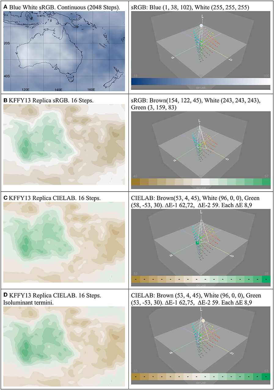
Figure 4. Comparative visualizations generated using Gradient Designer and LAB Color Mixer Apps (left column) shown with supporting insights in CIELAB color space provided through the GV_LAB App (right column). The grid values being displayed are taken from the 100 km depth slice (KFFY13). (A) Linearly interpolated HSL/sRGB reference view of the model in near-monochrome with slow values in dark blue; (B) Divergent 16 step RGB color-map replicating that used by KFFY13; (C) Divergent 16 step CIELAB interpolation replicating (B); (D) Divergent 16 step CIELAB interpolation with isoluminant end termini. All images assigned Generic RGB ICC profile. CIELAB colorspace conversions use D₆₅ 2° illuminant. High resolution: https://doi.org/10.5281/zenodo.3264037.

FIGURE 5

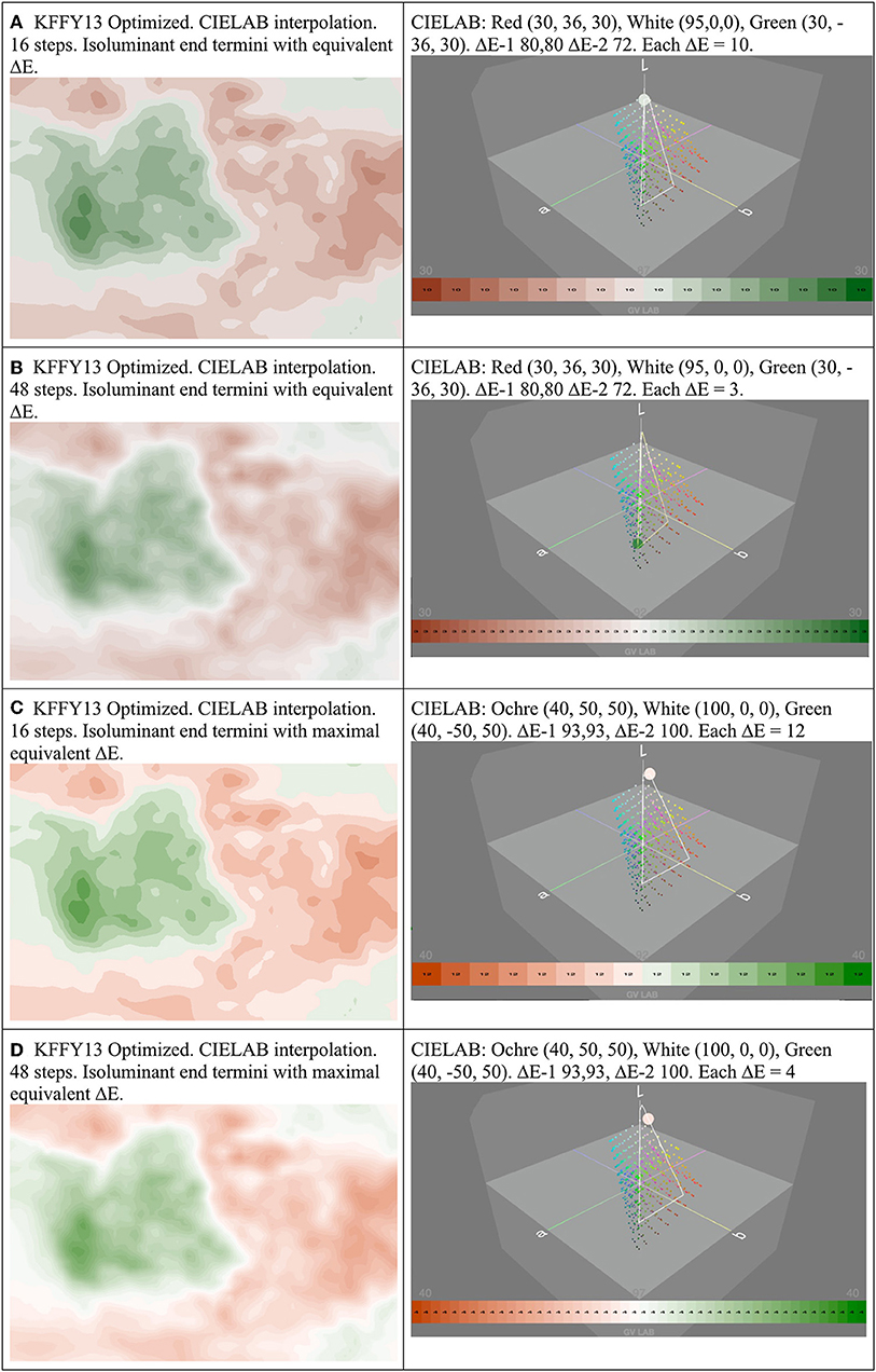
Figure 5. Comparative optimized visualizations generated using the Gradient Designer and LAB Color Mixer Apps (left column) shown with supporting insights in CIELAB color space provided through the GV_LAB App (right column). For details of the grid values being displayed, see the caption for Figure 4. (A) KFFY13 optimized, 16 step divergent color-map, with isoluminant termini with equivalent ΔE from termini to midpoint; (B) As per B, with 48 steps; (C) 16 step divergent color-map, with isoluminant termini with enlarged ΔE from termini to midpoint, enlarged ΔE between termini; (D) As per (C), with 48 steps. CIELAB colorspace conversions use D₆₅ 2° illuminant. Red-Green termini may present difficulties for viewers with deuteranopia, tritanopia. High resolution: https://doi.org/10.5281/zenodo.3264037.

FIGURE 6

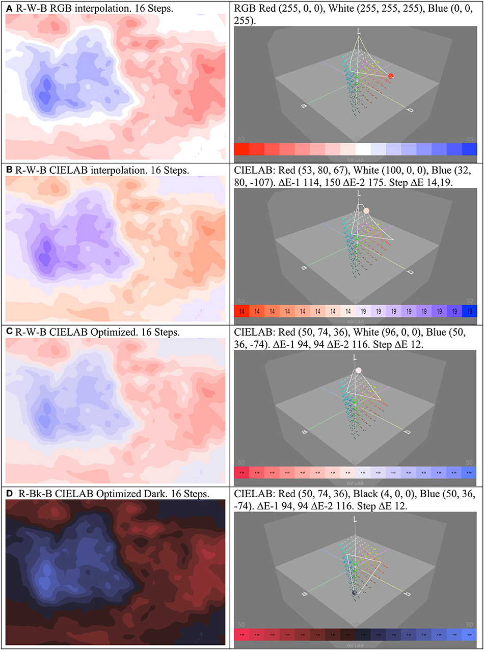
Figure 6. Further comparative visualizations generated using the Gradient Designer and LAB Color Mixer Apps (left column) shown with supporting insights in CIELAB color space provided through the GV_LAB App (right column). (A) R-W-B non-linear RGB interpolation 16 Steps; (B) R-W-B CIELAB interpolation 16 Steps. Red and Blue Values match 6 (A), Blue-White interpolation is sRGB gamut constrained; (C) R-W-B linear CIELAB Optimized 16 Steps, Red and Blue are Isoluminant (L = 50), all colors within sRGB gamut; (D) R-Bk-B CIELAB Optimized Dark 16 Steps. Red/Blue as per 6(C), Black L = 4. CIELAB colorspace conversions use D₆₅ 2° illuminant. High resolution: https://doi.org/10.5281/zenodo.3264037.

FIGURE 7

Figure 7. Detailed 2D Views and preparation for 3D. Visualizations generated using the Gradient Designer and LAB Color Mixer Apps (left column) shown with supporting insights in CIELAB color space provided through the GV_LAB App (right column). Note: images contain alpha channels composited against white background. (A) R-W-B gradient as per 6 (C), Center Alpha = 0; (B) R-Bk-B CIELAB Optimized Dark, 16 steps, Center Alpha = 0; (C) R-Bk-B CIELAB Optimized Dark, 48 steps, Center Alpha = 0; (D) R-Bk-B CIELAB Optimized Dark. 48 Steps. Left Alpha = 0. Center Alpha = 0. CIELAB colorspace conversions use D₆₅ 2° illuminant. High resolution: https://doi.org/10.5281/zenodo.3264037.

FIGURE 8

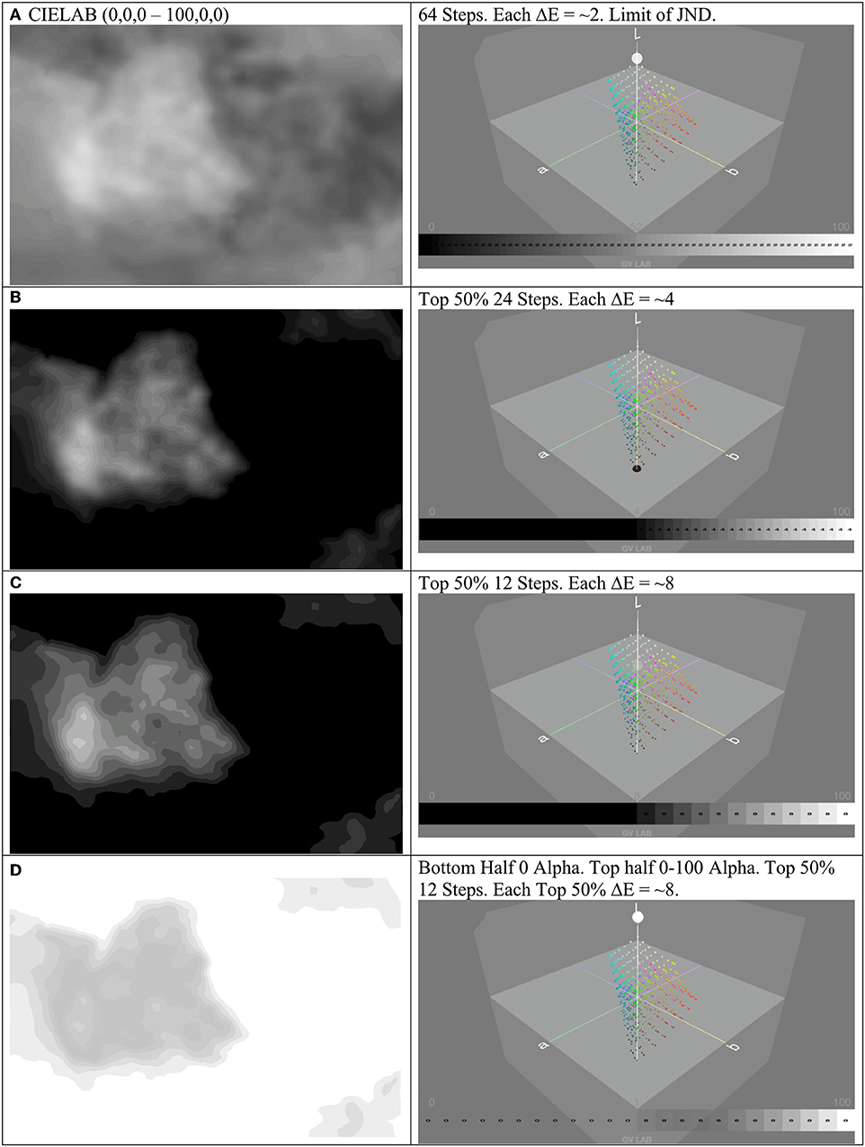
Figure 8. Comparative visualizations, intended to highlight areas of detail, generated using the Gradient Designer App (left column) shown with supporting insights in CIELAB color space provided through the GV_LAB App (right column). For details of the grid values being displayed, see the caption for Figure 4. (A) Detail All CIELAB 0-90 L 64 Steps. (B) Detail top-half CIELAB 0-90L 24 steps. (C) Detail top-half CIELAB 0-90L 12 steps. (D) Detail top-half CIELAB 0-90L 12 steps + bottom-half alpha 0, top-half alpha 0-100. CIELAB colorspace conversions use D₆₅ 2° illuminant. High resolution: https://doi.org/10.5281/zenodo.3264037.

The LAB color mixer directly displays the color difference values between each gradient terminus and the midpoint (ΔE-1, a value pair), the color difference between the two termini (ΔE-2) and ΔE across each interpolated color step. GV LAB visualizes isoluminance, color-map trajectories, ΔE and JNDs in CIELAB color space, clearly indicating the constraints of the sRGB (D₆₅) gamut. These are novel additions to the tools available to the researcher. The divergent sRGB color-map (Figure 4B) is replicated (Figure 4C) in CIELAB color space, with interval color values interpolated in that space using clearly enumerated ΔE values. In visualization Figure 4D, we equalize gradient termini located on an isoluminant AB plane (L = 53). This however, does not guarantee that the color intervals in the divergent three-point gradient cover equivalent Euclidean distance, nor that interpolated colors do not exceed the sRGB gamut.

In Figures 5A,B, we optimize the color-map, whilst maintaining the same general color range as Figure 4D, ensuring that all interpolated colors fall within the sRGB (D₆₅) gamut. Gradient termini are isoluminant (L = 30) and have equivalized ΔE-1 (= 80) for gradient termini. ΔE-2 (= 72) is also larger than that exhibited in Figure 4D (= 59). In Figures 5C,D we maximize both ΔE-1 (= 93) and ΔE-2 (= 100) for that region of the sRGB gamut (visualized by the isosceles triangles on the right column). This increases the dynamic range of the visualization both in lightness (L) and color difference (ΔE), and assures that Euclidean distances for gradient interpolation steps are equivalent, linearly matching the underlying data values. Figures 5C,D display results using 16 and 48 steps, with interpolated ΔE values of 12 and 4 respectively. These exceed recommended JND (>3) values for clearly discriminable colors, measurably indicating on which side (- or +) of the reference value they fall. They proceed in linear, quantifiable, perceptually accurate steps mapped to the underlying data values according to the CIELAB color model. At lower (16 steps) quantization the visualization performs categorically, where color steps implicitly consolidate wavespeed ranges and uncertainty. In concert with a higher dynamic range in L and ΔE, increased (finer) quantization acts like a lens, sharpening focus upon the underlying data, eliciting physical structural information to the extent this can be visually inferred within the limits of known uncertainty.

In Figures 6A–D Red-White-Blue divergent gradient colors are chosen to align with convention in seismology (i.e., reddish/orange colors represent slow wavespeeds; bluish colors represent fast wavespeeds). Terminal color values and their equivalents in different color spaces appear in Table 2. Following Kovesi (2015, p. 17), Figure 6A presents a standard RGB Red-White-Blue divergent gradient interpolated in RGB color space. Visualizing this in GV_LAB (right-hand column) in CIELAB color space clearly reveals this to be asymmetrical, non-linearly interpolated and volumetrically constrained by the sRGB gamut. Figure 6B replicates 6A in CIELAB colorspace, with Red/Blue terminal values per Table 2. Steps between termini are linearly interpolated within the sRGB volume, with Step ΔE-2 = 14,19. End termini to midpoint quantization constrains the point of closest interpolation to white. The gradient is non-optimal due to non-isoluminant end termini, sRGB volumetric constraint and asymmetry. None of the values in the underlying data map linearly to the Red/Blue extrema, implying that 6A is a poor representation.

TABLE 2

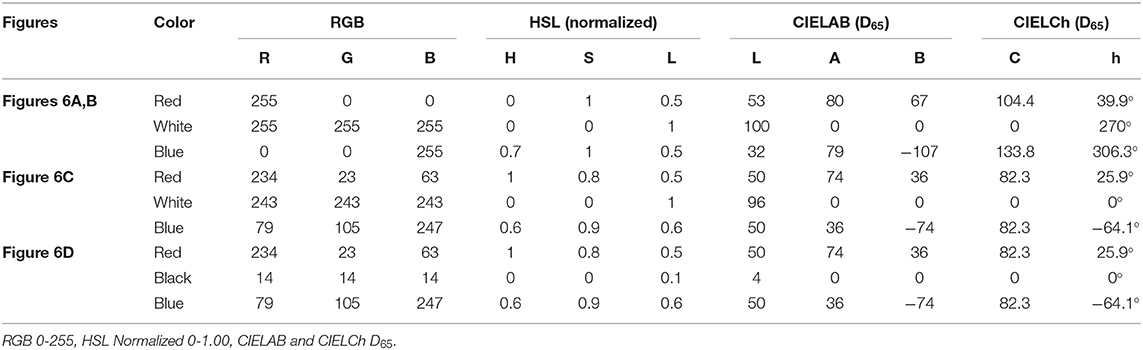
Table 2. Figures 6A–D Gradient Color Values.

Figure 6C optimizes 6B in CIELAB, adjusting color values to more closely match 6A. Red/Blue values are isoluminant (L = 50), all interpolated colors fall linearly (Step ΔE = 12) within the sRGB volume, forming a perceptually symmetrical gradient (ΔE-1 = 94, 94). The balanced dynamic range, linearly matching color differences and symmetry ensure a quantifiable perceptual match with underlying data values. Setting Red/Blue values to L = 50 also ensures that the gradient is easily invertible within the sRGB gamut.

Figure 6D sets the midpoint reference value to near Black (L = 4), and maintains Red/Blue CIELAB values from 6C. This maintains the ΔE-1, ΔE-2, and Steps ΔE of Figure 6C. It is perceptually near-equivalent to Figure 6C, with judiciously chosen termini within the complex shape of the sRGB volume. Invertibility of a gradient is a desirable characteristic for downstream 3D compositing methodologies (Porter and Duff, 1984), and should be tested for dynamic range and gamut exceedance at the outset of the design-decision process.

In Figures 7A–D, we introduce the ability of the LAB Color Mixer App to assign an interpolated alpha channel data to the gradient. This is not driven by underlying seismic wavespeed values directly, but by the user: the alpha channel is linearly interpolated across the number of gradient steps, and in this case enables specification of transparency. Figure 7A illustrates the non-linear interpolation this introduces when an alpha channel is applied to the optimized Red-White-Blue gradient. This is a consequence of the alpha blending function in OpenGL: multiplication of alpha values (0-1) applied to the relevant color values as L increases (Telea, 2007). Figure 7B demonstrates the retention of linearity when colors interpolate to black rather than white, affirming that an invertible divergent gradient is desirable for a variety of compositing approaches, dependent upon context and the compositing algorithm chosen. Figure 7C demonstrates the effect of finer gradient steps, which may be desirable in tomographic visualization. Finally, Figure 7D demonstrates the ability to display a selected range of the data (in this case the upper 50%) using alpha information, with the concomitant GV_LAB plot representing this as a straight line, as expected. These outputs are suitable for 3D compositing of multiple layers in external applications.

Our final visualizations in Figures 8A–D dispense with color and apply a simple greyscale gradient, linearly interpolated in CIELAB color space, with the intent to use lightness to reveal shape from shading. In this instance features emerge corresponding to regions of wavespeed contiguity and other structures of the mantle. Figure 8A illustrates the entire model with L ranging from 0 to 100, in 64 steps. This reduces the ΔE of each interpolated step to approximately 2, approaching the limit of JND for an expert observer. Figure 8B highlights the top 50% of the range, indicating regions of high wavespeed (24 steps), with each step ΔE = 4. A coarser approximation (12 steps) in Figure 8C reveals clear groupings within this subset, with a ΔE per step of ~8. Finally, Figure 8D introduces an alpha channel, applied at 100% for the lower 50% of the data, and linearly stepped from 0 to 100% over the top 50% range. This similarly prepares the output layers for 3D display.

Discussion

In the following section we note current limitations in our software and data visualization pipeline, followed by an appraisal of the strength of our approaches and the on-going potential for future research and development.

Implementing our software in the QC VPL limits our software to the MacOS platform. QC was chosen for its simple visual programming paradigm, its facility for rapid application prototyping and wide API support. Since 2018 QC has been deprecated by Apple, and future support is unclear. We intend to reimplement our software in an alternative VPL (e.g., Touch Designer, Derivative Inc., 2019) or a game engine environment (e.g., Unity Technologies, 2019), which include cross-platform support. Aspects of the UI can be improved subject to user-feedback. Future development could incorporate more sophisticated color models (e.g., CIECAM02; Fairchild, 2013), to account for known deficiencies with CIELAB. The 8-bit pipeline can be extended to 16- or 32-bit color and greyscale, including float as well as integer values for greater precision in the manipulation of continuous data. Improvements in alpha channel control could include evaluation of color-shift due to transparency mapping, extra functions for the alpha channel (e.g., tagging or delimiting regions, defining isosurfaces). Output improvements could include more control over Syphon/OSC output, including addressable transfer functions suitable for true volumetric raycasters and other shading models.

Our visualizations demonstrate that color-mapping should be conducted with great care and that extant mappings can be improved. Building on Kovesi (2015); Ware et al. (2018) and Crameri (2018a), we employed CIELAB color space to visualize continuous geoscience data.

We first showed a naive two color HSL/sRGB gradient reference visualization (Figure 4A) for the 100 km depth slice of the AuSREM model. Figure 4B closely replicated the sRGB KFFY13 100 km depth slice visualization incorporating uncertainty. Visualizing this gradient within the sRGB gamut mapped within CIELAB color space revealed the non-linear interpolation of the gradient. The gradient termini were re-mapped within CIELAB space, resulting in linear color interpolation between gradient termini. This revealed the difference in lightness (L) values between the end-point colors, in turn demonstrating that color differences between end termini and midpoint were non-equivalent. Using CIELAB color space we can accurately quantify this non-equivalence in ΔE values, both for the end-midpoint ranges and for the color difference of each step in the gradient. This causes the end points of the gradient to have different “perceptual distances” from the reference midpoint value, potentially creating the visual inference that regions of slower wavespeed are more proximate to the reference value than regions of higher wavespeed, when in fact this is not the case. Figure 4D adjusts for end-point isoluminance, but does not equalize ΔE, demonstrating that despite matching the L values of the endpoints, because color is used in the visualization, adjustments to color termini in the AB plane must also be undertaken in order to ensure gradient symmetry and matching of ΔE values.

Our software enabled us to control precisely and regularize these CIELAB differences, and to characterize uncertainty, using the ΔE metric. Isoluminant gradient termini, equidistant from the midpoint reference value, were established in Figure 5A. Figure 5B quantized the gradient from 16 to 48 steps, approaching the non-professional observer JND discriminability limit of 2 ≤ ΔE ≤ 3.5 per step. Whilst this exceeds our nominal uncertainty of +/− 0.05 kms⁻¹ per step, it affirms that coarser approximations will encode discriminable uncertainty across the gradient and consistently visually agglomerate regions according to a linear ΔE metric.

Optimizing for L and AB variation to elicit form, Figures 5C,D take advantage of the ability of our software to symmetrically maximize ΔE within the sRGB gamut. This demonstrates the capacity to linearly sharpen the chromatic distinction between steps, as well as maximizing lightness variation between end and midpoints of the gradient. This has the effect of enhancing contrast, shape perception and slow-fast discrimination across the data slice, whilst maintaining a JND of between ΔE = 12 and ΔE = 4, values that are well within the capabilities of the non-expert observer.

A standard seismic Red-White-Blue divergent gradient is optimized in Figures 6A,B, clearly demonstrating the non-linearity of this gradient if it is interpolated in RGB colorspace or naively transposed to CIELAB. This suggests that visualizations that naively use similar gradients may be misleading. Figure 6C represents a controlled, isoluminant, ΔE equivalized CIELAB version, with correct linear interpolation. The attraction of this approach is illustrated in Figure 6D, where the gradient is inverted, but is perceptually isometric. Isometric invertibility is attractive for 3D compositing operations, some 2D display and print operations, as well as for volumetric visualization.

Alpha is an important feature for compositing operations and may have unintended consequences for color perception. Figure 7 demonstrates the use of linearly interpolated alpha channels and their effect upon color values within CIELAB. Figures 7B,C demonstrates the retention of color interpolation linearity by the inverted gradient, which is desirable for additive or multiplicative compositing operations. ΔE values are disregarded when premultiplied alpha is applied. Figure 7D illustrates the capability of isolating value ranges through the use of alpha channel control.

The utility of CIELAB greyscale interpolation is demonstrated in Figure 8. Unlike perceptually non-uniform RGB greyscale interpolation, CIELAB greyscale is perceptually linear and midpoint gray is accurately represented (L = 50). The capability of LAB color mixer, GV_LAB and Gradient Designer is demonstrated in resolving the AusREM data from the limits of discriminability (Figure 8A), to the limits of known uncertainty (Figure 8B), along with the ability to isolate regions of interest (Figures 8C,D).

Visual inference may be one of the first important steps in ascertaining significant formal aspects of geoscientific data. Looking for structure in noisy or uncertain continuous data requires clarity and precision in analytical techniques, including color-mapping. Our software suite, repeatable metrics, and illustrative color-maps are a proof-of-concept that illuminate the relationships between data variables and color that should be part of visually-aware science and human-computer interaction for visual analytics. Interfaces for colorisation using perceptually uniform color spaces, such as CIELAB, provide greater certainty for the accurate visualization of data as well as enhancing the reproducibility of results.

Conclusions

We have demonstrated the subtle problems that the inherent non-uniformity of common RGB-based color models may present for the interpretation of scientific visualization. Our approach of color-mapping using the CIELAB color model improves the correspondence between a color-map and underlying data. We have demonstrated the capacity of interactive software to apply linear, quantifiable, and perceptually accurate color to a typical geoscience dataset, finding that:

1) Color should be applied to visualization of data with care.

2) CIELAB is a good choice of color space for colorization of linear data as it closely matches human color perception and facilitates a linear mapping between color space metrics and underlying data. Understanding that the sRGB gamut is a constrained subset of the CIELAB gamut is important knowledge. Visualization activities should take this constraint into account at the outset of the visualization process.

3) The ΔE metric accounts for linear color difference and establishes the limits of discriminability for color differences perceivable by the average observer. If color is to be interpolated across underlying data values, then this should take place within an appropriate linear color model, such as CIELAB, within the sRGB gamut.

4) Uncertainty can be characterized using ΔE. In this way, the visualization captures features of the data as well as implicitly representing the uncertainty, encoded as color difference.

5) Form is best expressed using lightness variation in CIELAB colorspace. Lightness can be linearly mapped to underlying data values, using dynamic range to elucidate spatial features. It may be used together with chromaticity or independently as greyscale. The interplay between chromaticity and lightness must be balanced in an effective visualization and may be explored using the software presented.

6) Reproducibility of color is enabled through the use of CIELAB. All color reproduction devices and media are susceptible to color variance. As a perceptual color space, CIELAB is an absolute color space with known values. Stipulating LAB and ΔE values for applied gradients in scientific visualization achieves the desirable goal of accurate color reproducibility across a range of platforms and media, such as calibrated computer displays and print devices.

7) Our contribution encourages attention to both “visual literacy” and “visual numeracy” for scientific data visualization. In providing software, raster image output files (.png), color palette files (.cpt) and data interchange outputs (JSON) that enable linear, quantifiable and perceptually accurate color, we hope to promote well-posed scientific visualization.

Data Availability Statement

Color-maps in raster image format (.png), color palette table (.cpt), and data interchange format (JSON), Gradient Designer software and companion applications are available for download from: https://doi.org/10.5281/zenodo.3264037.

Author Contributions

PM co-designed the study, developed the visualization software and wrote the text. AR co-designed the study and contributed to the text. TS carried out data pre-processing and contributed to the text.

Funding

PM acknowledges an RTP Scholarship from the University of Tasmania. TS acknowledges support under Australian Research Council's Special Research Initiative for Antarctic Gateway Partnership (Project ID SR140300001). This research was partly supported by the ARC Research Hub for Transforming the Mining Value Chain (project number IH130200004).

Conflict of Interest

The authors declare that the research was conducted in the absence of any commercial or financial relationships that could be construed as a potential conflict of interest.

Acknowledgments

The authors thank Paul Bourke for providing javascript programming expertise, Tom Ostersen for GMT expertise, and Stephen Walters for constructive feedback.

References

Anderson, M., Motta, R., Chandrasekar, S., and Stokes, M. (1996). “Proposal for a standard default color space for the internet – sRGB,” in Color and Imaging Conference, Vol. 1996 (Scottsdale, AZ: Society for Imaging Science and Technology), 238–245.

Google Scholar

Asano, Y., Fairchild, M. D., and Blondé, L. (2016). Individual colorimetric observer model. PLoS ONE 11:e0145671. doi: 10.1371/journal.pone.0145671

PubMed Abstract | CrossRef Full Text | Google Scholar

Bergman, L. D., Rogowitz, B. E., and Treinish, L. A. (1995). “A rule-based tool for assisting colormap selection,” in Proceedings of the 6th Conference on Visualization'95 (Atlanta, GA: IEEE Computer Society). doi: 10.1109/VISUAL.1995.480803

CrossRef Full Text | Google Scholar

Bertin, J. (1983). Semiology of Graphics: Diagrams, Networks, Maps, Vol. 1. Transl. by W. J. Berg. Madison, WI: University of Wisconsin Press.

Google Scholar

Brainard, D. H. (2003). “Color appearance and color difference specification,” in The Science of Color, ed S. K. Shevell (Amsterdam: Elsevier), 191–216. doi: 10.1016/B978-044451251-2/50006-4

CrossRef Full Text | Google Scholar

Buja, A., Cook, D., Hofmann, H., Lawrence, M., Lee, E.-K., Swayne, D. F., et al. (2009). Statistical inference for exploratory data analysis and model diagnostics. Philos. Trans. R. Soc. Lond. 367, 4361–4383. doi: 10.1098/rsta.2009.0120

PubMed Abstract | CrossRef Full Text | Google Scholar

Bujack, R., Turton, T. L., Samsel, F., Ware, C., Rogers, D. H., and Ahrens, J. (2018). The good, the bad, and the ugly: a theoretical framework for the assessment of continuous colormaps. IEEE Trans. Visual. Comput. Graph. 24, 923–933. doi: 10.1109/TVCG.2017.2743978

PubMed Abstract | CrossRef Full Text | Google Scholar

Butterworth, T., Marini, A., and Contributors, S. (2018). Syphon Framework [Objective-C, MacOS]. Available online at: https://github.com/Syphon/syphon-framework (accessed May 28, 2019).

Google Scholar

CIE (2004). Technical Report: Colorimetry, 3rd Edn, Vol. 15. Commission International de L'Eclairage.

Google Scholar

CIE (2007). Colorimetry — Part 4: CIE1976 L^*a^*b^* Colour Space. CIE. Available online at: http://www.cie.co.at/publications/colorimetry-part-4-cie-1976-lab-colour-space (accessed February 5, 2019).

Google Scholar

Cook, D. (2017). Myth Busting and Apophenia in Data Visualisation: Is What You See Really There? Available online at: http://dicook.org/talk/ihaka/ (accessed February 12, 2019).

Google Scholar

Cook, D., Lee, E.-K., and Majumder, M. (2016). Data visualization and statistical graphics in big data analysis. Annu. Rev. Stat. Appl. 3, 133–159. doi: 10.1146/annurev-statistics-041715-033420

CrossRef Full Text | Google Scholar

Crameri, F. (2018a). Geodynamic diagnostics, scientific visualisation and StagLab 3.0. Geosci. Model Dev. 11, 2541–2562. doi: 10.5194/gmd-11-2541-2018

CrossRef Full Text | Google Scholar

Crameri, F. (2018b). Scientific Colour Maps (Oslo). doi: 10.5281/zenodo.2649252

CrossRef Full Text | Google Scholar

Derivative Inc. (2019). Derivative TouchDesigner. Available online at: https://www.derivative.ca/ (accessed May 8, 2019).

PubMed Abstract | Google Scholar

Douglas, S. A., and Kirkpatrick, A. E. (1999). Model and representation: the effect of visual feedback on human performance in a color picker interface. ACM Trans. Graph. 18, 96–127. doi: 10.1145/318009.318011

CrossRef Full Text | Google Scholar

Eddins, S. (2014). Rainbow Color Map Critiques: An Overview and Annotated Bibliography. Available online at: https://au.mathworks.com/company/newsletters/articles/rainbow-color-map-critiques-an-overview-and-annotated-bibliography.html (accessed July 2, 2019).

Google Scholar

Eisemann, M., Albuquerque, G., and Magnor, M. (2011). “Data driven color mapping,” in Proceedings of EuroVA: International Workshop on Visual Analytics (Bergen: Eurographics Association).

Google Scholar

Fairchild, M. D. (2013). Color Appearance Models. Chichester, UK: John Wiley and Sons. doi: 10.1002/9781118653128

PubMed Abstract | CrossRef Full Text | Google Scholar

Foster, D. H.(eds.). (2008). “Color appearance,” in The Senses: A Comprehensive Reference, Vol. 2, eds A. Basbaum, A. Kaneko, G. Shepherd, G. Westheimer, T. Albright, and R. Masland (San Diego, CA: Academic Press), 119–132. doi: 10.1016/B978-012370880-9.00303-0

CrossRef Full Text | Google Scholar

Gordon, I. E. (2004). Theories of Visual Perception, 3 Edn. Hove: Psychology Press. doi: 10.4324/9780203502259

CrossRef Full Text | Google Scholar

Haber, R. B., and McNabb, D. A. (1990). Visualization idioms: a conceptual model for scientific visualization systems. Visual. Sci. Comput. 74:93.

Google Scholar

Hansen, C. D., and Johnson, C. R. (eds.). (2005). The Visualization Handbook. Boston, MA: Elsevier-Butterworth Heinemann.

Google Scholar

Harold, J., Lorenzoni, I., Shipley, T. F., and Coventry, K. R. (2016). Cognitive and psychological science insights to improve climate change data visualization. Nat. Clim. Change 6, 1080–1089. doi: 10.1038/nclimate3162

CrossRef Full Text | Google Scholar

Hawkins, E. (2015). Graphics: scrap rainbow colour scales. Nature 519:291. doi: 10.1038/519291d

PubMed Abstract | CrossRef Full Text | Google Scholar

Healey, C. G., and Enns, J. T. (2012). Attention and visual memory in visualization and computer graphics. Visual. Computer Graph. IEEE Trans. 18, 1170–1188. doi: 10.1109/TVCG.2011.127

PubMed Abstract | CrossRef Full Text | Google Scholar

Hoffmann, G. (2000). CIE Color Space [Professional]. Available online at: http://www.docs-hoffmann.de/ciexyz29082000.pdf (accessed July 2, 2019).

Google Scholar

Hoffmann, G. (2008). CIELab Color Space [Professional]. Available online at: http://www.docs-hoffmann.de/cielab03022003.pdf (accessed July 2, 2019).

Google Scholar

Hunter Associates Laboratory Inc. (2018). Brief Explanation of delta E or delta E^*. Available online at: http://support.hunterlab.com/hc/en-us/articles/203023559-Brief-Explanation-of-delta-E-or-delta-E- (accessed February 18, 2019).

Google Scholar

IEC (1999). IEC 61966-2-1:1999. Multimedia Systems and Equipment - Colour Measurement and management - Part 2-1: Colour Management - Default RGB Colour Space - sRGB. Available online at: https://webstore.iec.ch/publication/6169 (accessed May 3, 2019).

Google Scholar

IRO Group Ltd (2019). Math|EasyRGB. Available online at: http://www.easyrgb.com/en/math.php (accessed May 23, 2019).

Google Scholar

Keim, D. A. (2001). Visual exploration of large data sets. Commun. ACM 44, 38–44. doi: 10.1145/381641.381656

CrossRef Full Text | Google Scholar

Keim, D. A., Kohlhammer, J., Ellis, G., and Mansmann, F. (2010). “Mastering the information age solving problems with visual analytics,” in Eurographics, eds D. Keim, J. Kohlhammer, G. Ellis, and F. Mansmann. Retrieved from: http://diglib.eg.org

Google Scholar

Keim, D. A., Mansmann, F., Schneidewind, J., and Ziegler, H. (2006). “Challenges in visual data analysis,” in Tenth International Conference on Information Visualisation (IV'06) (London, UK), 9–16. doi: 10.1109/IV.2006.31

CrossRef Full Text | Google Scholar

Kennett, B. L. N., Engdahl, E. R., and Buland, R. (1995). Constraints on seismic velocities in the Earth from traveltimes. Geophys. J. Int. 122, 108–124. doi: 10.1111/j.1365-246X.1995.tb03540.x

CrossRef Full Text | Google Scholar

Kennett, B. L. N., Fichtner, A., Fishwick, S., and Yoshizawa, K. (2013). Australian Seismological Reference Model (AuSREM): mantle component. Geophys. J. Int. 192, 871–887. doi: 10.1093/gji/ggs065

CrossRef Full Text | Google Scholar

Kovesi, P. (2015). Good colour maps: how to design them. arxiv:1509.03700 [Cs]. Available online at: http://arxiv.org/abs/1509.03700 (accessed May 28, 2019).

Google Scholar

Light, A., and Bartlein, P. J. (2004). The end of the rainbow? Color schemes for improved data graphics. Eos Trans. Am. Geophys. Union 85, 385–391. doi: 10.1029/2004EO400002

CrossRef Full Text | Google Scholar

Lindbloom, B. (2013). Useful Color Equations. Available online at: http://www.brucelindbloom.com/index.html (accessed February 18, 2019).

Google Scholar

Lindbloom, B. (2017). Delta E (CIE 1976). Retrieved from: http://www.brucelindbloom.com/index.html?Eqn_DeltaE_CIE76.html (accessed February 18, 2019).

Google Scholar

Liu, S., Cui, W., Wu, Y., and Liu, M. (2014). A survey on information visualization: recent advances and challenges. Vis. Comput. 30, 1373–1393. doi: 10.1007/s00371-013-0892-3

CrossRef Full Text | Google Scholar

Luo, M. R., Cui, G., and Li, C. (2006). Uniform colour spaces based on CIECAM02 colour appearance model. Color Res. Appl. 31, 320–330. doi: 10.1002/col.20227

CrossRef Full Text | Google Scholar

MacEachren, A. M., Roth, R. E., O'Brien, J., Li, B., Swingley, D., and Gahegan, M. (2012). Visual semiotics and uncertainty visualization: an empirical study. IEEE Trans. Visual. Comput. Graph. 18, 2496–2505. doi: 10.1109/TVCG.2012.279

PubMed Abstract | CrossRef Full Text | Google Scholar

Masaoka, K., Berns, R. S., Fairchild, M. D., and Moghareh Abed, F. (2013). Number of discernible object colors is a conundrum. J. Opt. Soc. Am. 30:264. doi: 10.1364/JOSAA.30.000264

PubMed Abstract | CrossRef Full Text | Google Scholar

Meier, B. J., Spalter, A. M., and Karelitz, D. B. (2004). Interactive color palette tools. IEEE Comput. Graph. Appl. 24, 64–72. doi: 10.1109/MCG.2004.1297012

PubMed Abstract | CrossRef Full Text | Google Scholar

Meyer, G. W., and Greenberg, D. P. (1980). Perceptual color spaces for computer graphics. ACM SIGGRAPH Comput. Graph. 14, 254–261. doi: 10.1145/965105.807502

CrossRef Full Text | Google Scholar

Milgram, P., and Kishino, F. (1994). “A taxonomy of mixed reality visual displays,” in IEICE Transactions on Information System E77-D(12) (Tokyo), 16.

Google Scholar

Mittelstädt, S., and Keim, D. A. (2015). Efficient contrast effect compensation with personalized perception models. Comput. Graph. Forum 34, 211–220. doi: 10.1111/cgf.12633

CrossRef Full Text | Google Scholar

Mokrzycki, W. S., and Tatol, M. (2011). Colour difference ΔE - A survey. Mach. Graph. Vis. 20, 383–411. Retrieved from: https://www.researchgate.net/publication/236023905_Color_difference_Delta_E_-_A_survey (accessed October 15, 2019).

Google Scholar

Moreland, K. (2016). Why we use bad color maps and what you can do about it. Electron. Imaging 2016, 1–6. doi: 10.2352/ISSN.2470-1173.2016.16.HVEI-133

CrossRef Full Text | Google Scholar

Morovic, J., and Luo, M. R. (2001). The fundamentals of gamut mapping: a survey. J. Imaging Sci. Technol. 45, 283–290. Retrieved from: https://www.researchgate.net/publication/236121201_The_Fundamentals_of_Gamut_Mapping_A_Survey (accessed October 15, 2019).

Google Scholar

Morse, P. E. (2019). Pemorse/Data-Visualisation-Tools: Gradient Designer Suite. V.0.9-Alpha Release. Hobart, TAS. doi: 10.5281/zenodo.3264037

CrossRef Full Text | Google Scholar

Morse, P. E., and Bourke, P. D. (2012). “Hemispherical dome adventures,” Presented at iVEC (University of Western Australia). Retrieved from: http://rgdoi.net/10.13140/RG.2.2.15942.16963

Google Scholar

Munzner, T. (2014). Visualization Analysis and Design. Boca Raton, FL: A. K. Peters/CRC Press.

Google Scholar

NewTek (2019). NewTek NDI Tools. Available online at: https://www.newtek.com/ndi/tools/ (accessed February 22, 2019).

Google Scholar

Porter, T., and Duff, T. (1984). Compositing digital images. Comput. Graph. 18:7. doi: 10.1145/964965.808606

CrossRef Full Text | Google Scholar

Poynton, C. A. (1994). “Wide gamut device-independent colour image interchange,” in International Broadcasting Convention - IBC '94 (Amsterdam), 218–222. doi: 10.1049/cp:19940755

CrossRef Full Text | Google Scholar

Poynton, C. A. (2006). Frequently asked questions about color [Professional]. Available online at: http://poynton.ca/ColorFAQ.html (accessed May 28, 2019).

Google Scholar

Poynton, C. A. (2012). Digital Video and HD: Algorithms and Interfaces. Amsterdam: Elsevier. doi: 10.1016/B978-0-12-391926-7.50063-1

CrossRef Full Text | Google Scholar

Rawlinson, N., Reading, A. M., and Kennett, B. L. N. (2006). Lithospheric structure of Tasmania from a novel form of teleseismic tomography. J. Geophys. Res. 111:B02301. doi: 10.1029/2005JB003803

CrossRef Full Text | Google Scholar

Rheingans, P. (1992). “Color, change, and control of quantitative data display,” in IEEE Conference on Visualization, 1992, Visualization'92 (Boston, MA: IEEE), 252–259. doi: 10.1109/VISUAL.1992.235201

CrossRef Full Text | Google Scholar

Rheingans, P. (2000). “Task-based color scale design,” in 28th AIPR Workshop: 3D Visualization for Data Exploration and Decision Making, Vol. 3905, 35–44. Retrieved from: http://proceedings.spiedigitallibrary.org/proceeding.aspx?articleid=916058

Google Scholar

Rheingans, P., and Tebbs, B. (1990). A tool for dynamic explorations of color mappings. ACM SIGGRAPH Comput. Graph. 24, 145–146. doi: 10.1145/91394.91436

CrossRef Full Text | Google Scholar

Robertson, P. K. (1988). Visualizing color gamuts: a user interface for the effective use of perceptual color spaces in data displays. IEEE Comput. Graph. Appl. 8, 50–64. doi: 10.1109/38.7761

CrossRef Full Text | Google Scholar

Rogowitz, B. E., and Goodman, A. (2012). “Integrating human- and computer-based approaches for feature extraction and analysis,” in Proceedings of the SPIE (Burlingame, CA), 8291. doi: 10.1117/12.915887

CrossRef Full Text | Google Scholar

Rogowitz, B. E., and Treish, L. A. (1998). Data visualisation: the end of the rainbow. IEEE Spectr. 35, 52–59. doi: 10.1109/6.736450

CrossRef Full Text | Google Scholar

Rougier, N. P., Droettboom, M., and Bourne, P. E. (2014). Ten simple rules for better figures. PLoS Computat. Biol. 10:e1003833. doi: 10.1371/journal.pcbi.1003833

PubMed Abstract | CrossRef Full Text | Google Scholar

Schulz, H., Nocke, T., Heitzler, M., and Schumann, H. (2013). A design space of visualization tasks. IEEE Trans. Visual. Comput. Graph. 19, 2366–2375. doi: 10.1109/TVCG.2013.120

PubMed Abstract | CrossRef Full Text | Google Scholar

Sharma, G., and Rodriguez-Pardo, C. E. (2012). “The dark side of CIELAB,” in Color Imaging XVII: Displaying, Processing, Hardcopy, and Applications, Vol. 8292. Available online at: http://www.hajim.rochester.edu/ece/~gsharma/papers/SharmaDarkSideColorEI2012.pdf (accessed May 28, 2019).

Google Scholar

Sharma, G., and Trussell, H. J. (1997). Digital color imaging. IEEE Trans. Image Process. 6, 901–932. doi: 10.1109/83.597268

PubMed Abstract | CrossRef Full Text | Google Scholar

Silva, S., Sousa Santos, B., and Madeira, J. (2011). Using color in visualization: a survey. Comput. Graph. 35, 320–333. doi: 10.1016/j.cag.2010.11.015

CrossRef Full Text | Google Scholar

Smith, A. R. (1978). Color gamut transform pairs. ACM Siggraph Comput. Graph. 12, 12–19. doi: 10.1145/965139.807361

CrossRef Full Text | Google Scholar

Smith, N., van der Walt, S., and Firing, E. (2015). Matplotlib Colormaps. Available online at: https://matplotlib.org/tutorials/colors/colormaps.html (accessed May 28, 2019).

Google Scholar

Stål, T. (2019). TobbeTripitaka/Grid: First Frame (Version 0.3.0). Available online at: http://doi.org/10.5281/zenodo.2553966 (accessed May 28, 2019).

Google Scholar

Stauffer, R., Mayr, G. J., Dabernig, M., and Zeileis, A. (2015). Somewhere over the rainbow: how to make effective use of colors in meteorological visualizations. Bull. Am. Meteorol. Soc. 96, 203–216. doi: 10.1175/BAMS-D-13-00155.1

CrossRef Full Text | Google Scholar

Stockman, A., and Brainard, D. H. (2015). “Fundamentals of color vision I: color processing in the eye,” in Handbook of Color Psychology, eds A. J. Elliot, M. D. Fairchild, and A. Franklin (Cambridge, UK: Cambridge University Press), 27–69. doi: 10.1017/CBO9781107337930.004

CrossRef Full Text | Google Scholar

Telea, A. C. (2007). Data Visualization: Principles and Practice. Boca Raton, FL: AK Peters; CRC Press. doi: 10.1201/b10679

CrossRef Full Text | Google Scholar

Tkalcic, M., and Tasic, J. F. (2003). “Colour spaces: perceptual, historical and applicational background,” in The IEEE Region 8 EUROCON 2003 Computer as a Tool (Ljubljana), 304–308.

Google Scholar

Tufte, E. R. (1990). Envisioning Information. Cheshire, CT: Graphics Press.

Google Scholar

Tukey, J. W. (1977). Exploratory Data Analysis, Vol. 2. Reading, MA: Addison-Wesley.

Google Scholar

Tukey, J. W. (1990). Data-based graphics: visual display in the decades to come. Stat. Sci. 5, 327–339. doi: 10.1214/ss/1177012101

CrossRef Full Text | Google Scholar

Unity Technologies (2019). Unity. Available online at: https://unity.com/frontpage

PubMed Abstract | Google Scholar

Van Wijk, J. J. (2005). “The value of visualization,” in Visualization, 2005. VIS 05 (Minneapolis, MN: IEEE), 79–86. doi: 10.1109/VISUAL.2005.1532781

CrossRef Full Text | Google Scholar

Ward, M. O., Grinstein, G., and Keim, D. (2010). Interactive Data Visualization: Foundations, Techniques, and Applications. Natick, MA: AK Peters; CRC Press. doi: 10.1201/b10683

CrossRef Full Text | Google Scholar

Ware, C. (1988). Color sequences for univariate maps: theory, experiments and principles. IEEE Comput. Graph. Appl. 8, 41–49. doi: 10.1109/38.7760

CrossRef Full Text | Google Scholar

Ware, C. (2013). Information Visualization: Perception for Design, 3rd Edn. Amsterdam: Elsevier.

Google Scholar

Ware, C., Turton, T. L., Bujack, R., Samsel, F., Shrivastava, P., and Rogers, D. H. (2018). Measuring and modeling the feature detection threshold functions of colormaps. IEEE Trans. Vis. Comput. Graph. 25, 2777–2790. doi: 10.1109/TVCG.2018.2855742

PubMed Abstract | CrossRef Full Text | Google Scholar

Wessel, P., Smith, W. H. F., Scharroo, R., Luis, J., and Wobbe, F. (2013). Generic mapping tools: improved version released. Eos Trans. Am. Geophys. Union 94, 409–410. doi: 10.1002/2013EO450001

CrossRef Full Text | Google Scholar

Wickham, H., Cook, D., Hofmann, H., and Buja, A. (2010). Graphical inference for infovis. IEEE Trans. Visual. Comput. Graph. 16, 973–979. doi: 10.1109/TVCG.2010.161

PubMed Abstract | CrossRef Full Text | Google Scholar

Wilkinson, L. (2005). The Grammar of Graphics, 2nd Edn. Chicago, IL: Springer Science and Business Media.

Google Scholar

Wyszecki, G., and Stiles, W. S. (1982). Color Science, Vol. 8. New York, NY: Wiley.

Google Scholar

Zeileis, A., and Hornik, K. (2006). Choosing Color Palettes for Statistical Graphics (No. 41). Vienna: Department of Statistics and Mathematics, WU Vienna University of Economics and Business. Retrieved from: http://epub.wu.ac.at/1404/

Google Scholar

Zeyen, M., Post, T., Hagen, H., Ahrens, J., Rogers, D., and Bujack, R. (2018). Color Interpolation for Non-Euclidean Color Spaces. Berlin: IEEE. doi: 10.1109/SciVis.2018.8823597

CrossRef Full Text | Google Scholar

Zhou, L., and Hansen, C. D. (2016). A survey of colormaps in visualization. IEEE Trans. Visual. Comput. Graph. 22, 2051–2069. doi: 10.1109/TVCG.2015.2489649

PubMed Abstract | CrossRef Full Text | Google Scholar