Satellite Data Reveal Cropland Losses in South-Eastern Ukraine Under Military Conflict

Introduction

In 2013–2014, Ukraine experienced a dramatic political and social change, caused by the annexation of Crimea by the Russian Federation, and partial occupation of areas in Donetsk and Luhansk regions by pro-Russian militants (Ivanov, 2015; Davis, 2016). The ongoing military conflict in these regions has had a considerable socio-economic impact in the area, including migration (1.5 M people were displaced internally) (Woroniecka-Krzyzanowska and Palaguta, 2016), health (Vasylyeva et al., 2018) and economy (Davis, 2016). From 2009 to 2013, the Donetsk and Luhansk regions (53.2 thousand sq. km, or 8.8% of total Ukraine area) accounted for c. 16% of total Ukrainian gross domestic product (GDP), according to the State Statistics Service of Ukraine (SSSU) (Figure 1). However, as of now, only 68% of Donetsk region and 69% of Luhansk region are under control by the Ukrainian Government (Figure 2), and their share in national GDP dropped to 7.5% between 2014 and 2017. Although only half of the area of these regions is cropland, agriculture contributed 4.1% (Donetsk) and 5.9% (Luhansk) to the overall regional gross value added (GVA) in 2009–2013 (Figure 1). With industrial decline between 2014 and 2017 due to the ongoing conflict, agriculture’s contribution to GVA increased to 7.6% in the Donetsk region and 18.6% in the Luhansk region. With the increased role of agriculture in the regional economy, it is important to understand how the ongoing conflict is impacting agricultural land use and the geographical patterns of these changes. The collapse of the former Soviet Union led to land use change in the Ukraine in the form of cropland abandonment (Gutman and Radeloff, 2016; Lesiv et al., 2018). However, since 2007, these abandoned agricultural lands started to be re-cultivated, resulting in up to 1 million ha of re-cultivation (Smaliychuk et al., 2016).

FIGURE 1

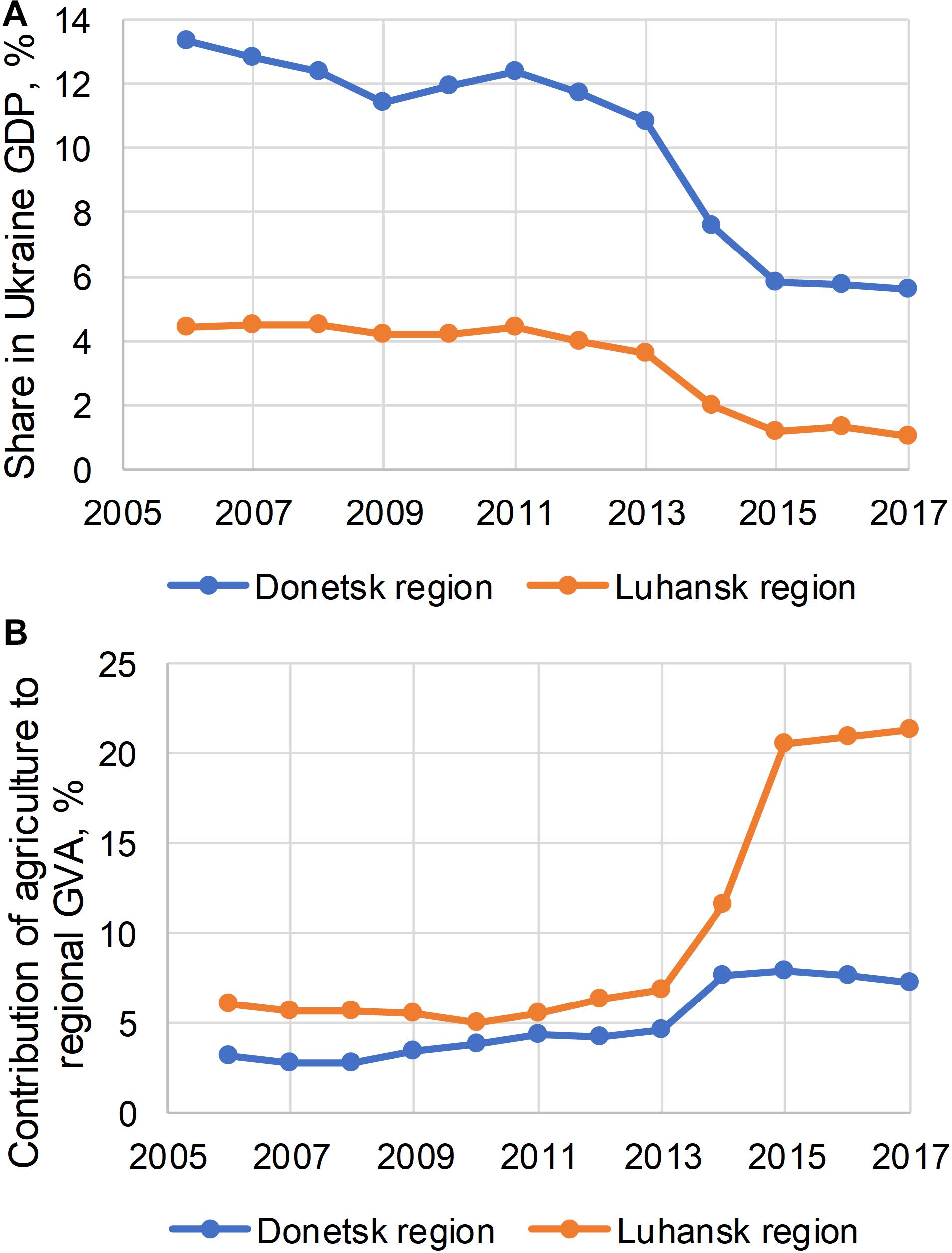
Figure 1. Dynamics of some economic metrics in Donetsk and Luhansk regions in 2006–2017. Share of the regions in Ukrainian gross domestic product (GDP) (A). Contribution of agriculture to gross value added (GVA) for Donetsk and Luhansk regions (B). Data were obtained from Statistical Bulletin “Gross Regional Product in 2017,” produced by SSSU.

FIGURE 2

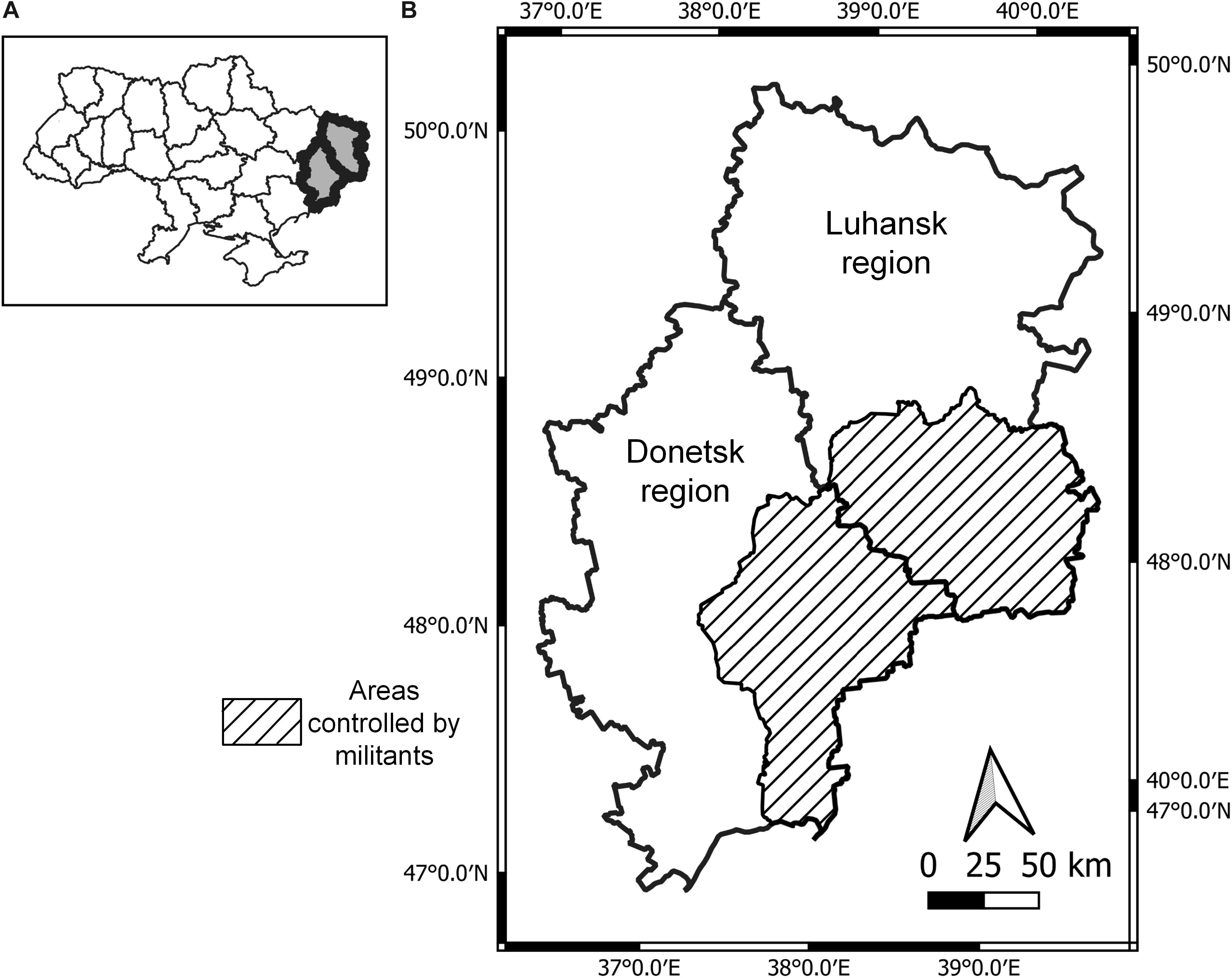
Figure 2. Location of Donetsk and Luhansk regions in Ukraine (A). Areas under control by the Ukrainian Government and militants (B). Location of the conflict border line was obtained from the official map produced by the Ministry of Defense of Ukraine (http://www.mil.gov.ua/en/news/2019/02/18/briefing-of-the-english- spokesman-of-the-ministry-of-defence-of-ukraine-(video)/).

However, no studies have been undertaken on quantifying LCLU changes in the Donetsk and Luhansk regions due to the recent military conflict. This is in part due to the lack of reliable information, especially in the regions not under control of the Ukrainian Government. The SSSU does not provide any statistical data in the regions under control by the militants, and collection of data becomes practically impossible due to the ongoing combat activities. Therefore, remote observations from space, provide a viable alternative source of information with regular, timely and synoptic coverage of these regions. In this study, we used freely available data acquired by remote sensing satellites, namely Landsat-7 (Arvidson et al., 2001), Landsat-8 (Roy et al., 2014), and Sentinel-2 (Drusch et al., 2012), to map cropland areas in the Donetsk and Luhansk regions at 30-m spatial resolution in 2013 (before the conflict) and 2018 (during the conflict). We use the definition of “cropland,” adopted within the Joint Experiment for Crop Assessment and Monitoring (JECAM) network, which defines cropland a piece of land that is sown/planted and harvestable at least once within the 12 months after the sowing/planting date (Waldner et al., 2016). Since satellite-derived maps have errors and provide biased estimates of areas, we combine those maps with sample-based reference data to derive unbiased area estimates along with uncertainties (Stehman, 2013; Olofsson et al., 2014). The derived LCLU maps allow us not only to quantify overall changes of cropland areas in the regions, but also analyze regional patterns and transitions with other LCLU classes.

Materials and Methods

Experimental Design

Experimental design to estimate areas of cropland change followed well-established recommended practices (Stehman, 2013; Olofsson et al., 2014). Multi-temporal multi-spectral satellite data at 30-m spatial resolution were used to classify the territory of Donetsk and Luhansk regions into cropland and non-cropland areas for 2013 and 2018. These maps were used to generate a change detection map with four classes: “Stable non-cropland” (non-cropland areas in both 2013 and 2018), “Stable cropland” (cropland areas in both 2013 and 2018), “Cropland gain” (non-cropland in 2013 and cropland in 2018), and “Cropland loss” (cropland in 2013 and non-cropland in 2018). Areas of cropland changes were estimated from samples. A stratified random sampling approach was employed with four classes from the change detection map used as strata. Each sample represented a 30 × 30 m pixel, and was labeled through photo-interpretation by an expert. For this, very high spatial resolution (VHR) imagery from Google Earth and time-series of moderate spatial resolution satellite imagery (Landsat-7, Landsat-8, and Sentinel-2) were analyzed visually to label each sampled pixel into cropland or non-cropland class in 2013 and 2018. The samples were used to calculate a confusion matrix in terms of area proportions. Finally, proportions of areas derived from samples (a stratified estimator, when map classes are strata) were used to estimate areas and corresponding standard errors (Stehman, 2013; Olofsson et al., 2014). The overall flowchart is show in Supplementary Figure 1.

Satellite Data

Remote sensing images acquired by the Enhanced Thematic Mapper Plus (ETM+) instrument aboard Landsat-7 satellite, the Operational Land Imager (OLI) instrument aboard Landsat-8 satellite and by the Multi-Spectral Instrument (MSI) aboard Sentinel-2A/B satellites were used in the study. Time-series of Landsat-7/ETM+ and Landsat-8/OLI data were used for cropland mapping in 2013, and Landsat-8/OLI and Sentinel-2A/B were used for cropland mapping in 2018. Landsat-7/ETM + captures images of the Earth’s surface in 7 spectral bands at 30 m spatial resolution (15 m for panchromatic band); Landsat 8/OLI acquires images in nine spectral bands at 30 m spatial resolution (15 m for panchromatic band); and Sentinel-2A/B/MSI acquire images in 13 spectral bands at 10, 20, and 60 m spatial resolution. For 2013, atmospherically corrected Landsat-7/ETM+ and Landsat-8/OLI data (Level-2 data product) were downloaded from the USGS’ EarthExplorer system. For 2018, we used NASA’s Harmonized Landsat Sentinel-2 (HLS) product (Claverie et al., 2018), which provides a Level-2 Nadir BRDF (Bidirectional Reflectance Distribution Function)-Adjusted surface Reflectance (NBAR) at 30 m spatial resolution. Satellite images were further re-projected to the Albers Equal Area projection at 30 m and mosaiced to cover the study area. Both USGS and HLS products provide quality assessment (QA) layers that were used to eliminate clouds and shadows from satellite imagery. Since data availability varied in 2013 and 2018 (with much more frequent observations available in 2018), different strategies were used to generate composites of surface reflectance values, which were ultimately used as features for cropland mapping. These composites were also generated with respect to the phenology of winter and summer crops. Winter crops are usually planted in September–October of the preceding year, and re-emerge in early spring after the dormancy period in winter. Winter crops are typically harvested in July. Summer crops are typically planted in April–May and harvested in August–September.

In 2013, three time periods were used to capture cropland developments during the growing season (Supplementary Figure 2): March 1–May 31, June 1–August 31, and July 1–August 31. The compositing was performed using a maximum normalized difference vegetation index (NDVI) approach (Holben, 1986), where an observation with maximum NDVI during the specified period is used in the temporal composite. For 2018, owing to more frequent observations from Landsat-8/OLI and Sentinel-2A/B (Li and Roy, 2017), the following time periods were used (Supplementary Figure 3): April 9, May 4, June 18, July 7–13, August 24–27, and September 24. For cropland mapping, we used time-series of surface reflectance values in the following six spectral bands: blue (∼0.480 μm), green (∼0.560 μm), red (∼0.660 μm), near infrared (NIR) (∼0.865 μm), and two short-wave infrared (SWIR) (∼1.6 μm and ∼2.2 μm).

Topography Data

One arc-second digital elevation model (DEM) derived from the Shuttle Radar Topography Mission (SRTM) (Farr et al., 2007) was used as an additional input for cropland mapping. The DEM was re-projected to Albers Equal Area projection at 30 m resolution to match optical satellite data, and three features were derived, namely elevation, slope and aspect.

Reference Data Generation

Reference data for cropland mapping (training dataset) and area estimation (samples) were generated through photo-interpretation by an expert by analyzing moderate spatial resolution data (Landsat-7, Landsat-8, and Sentinel-2) and VHR data available at Google Earth. The reference data were classified into two classes (cropland and non-cropland) through analysis of satellite image time-series, which capture phenological development of cropland, as well as spatial textural information from the VHR satellite data. Usually availability of the VHR images in the May-August period allowed better detection of agricultural fields. In cases, where VHR data were not available, only time-series of moderate spatial resolution data were used. The main difficulties were in discriminating cropland from natural vegetation. Multi-year natural vegetation can be discriminated from cultivated areas by their characteristic geometrical shape and boundaries. A more complex case is identification of abandoned fields with natural vegetation. This was done by first examining textural information from VHR imagery, as well as phenological profiles from moderate spatial resolution satellite data. Examples of abandoned fields with natural vegetation are given in Supplementary Figure 6.

Cropland Mapping

Multi-temporal optical satellite images in six spectral bands along with three DEM features (elevation, slope, and aspect) were concatenated into a feature vector that was input to the classifier. Before feeding into a classifier, input data were normalized to have mean 0 and standard deviation 1. We used a multi-layer perceptron (MLP) (Skakun et al., 2015; Kussul et al., 2017b) to classify each pixel into a cropland or non-cropland class. The MLP had 100 neurons in a hidden layer with a rectified linear unit (ReLU) activation function (Nair and Hinton, 2010) and two output neurons corresponding to two output classes. To reduce MLP overfitting, we also applied an L₂ (or Tikhonov’s) regularization (Phillips, 1962; Tikhonov et al., 1998). The derived cropland extent maps were filtered to remove connected objects, identified as cropland, with an area nine pixels or less. Binary cropland/non-cropland maps for 2013 and 2018 were used to derive the cropland change map with the following four classes: stable non-cropland, stable cropland, cropland gain and cropland loss. The majority voting filter with a 3 × 3 kernel was run for the change detection map to reduce the impact of noise and isolated pixels.

Area Estimation

The maps incorporate errors and direct application of maps for area estimation, for example pixel counting, will result in biased estimates. A stratified random sampling of 30 × 30 m pixels was used to estimate the areas of cropland change. Four strata were identified from the satellite derived 2013–2018 cropland change detection map: “Stable non-cropland,” “Stable cropland,” “Cropland gain,” and “Cropland loss.” Overall, 831 samples (sampling rate was 0.0014%) were used with 308 samples allocated for strata “Stable non-cropland,” 220 samples for “Stable cropland,” 126 samples for “Cropland gain,” and 177 samples for “Cropland loss.” The number of samples was selected in the following way: 75 and 100 samples were initially allocated for change strata “Cropland gain” and “Cropland loss,” respectively, while the remainder of the sample size was allocated proportionally to the area of the corresponding stratum. Pre-allocating a certain number of samples for change strata was done to reduce uncertainties of area estimates for change strata (Olofsson et al., 2014). These samples were used to compute confusion matrices to estimate the accuracies of the map, estimate the areas and corresponding uncertainties (Olofsson et al., 2014). These estimates are given in Supplementary Data Sheet 1.

Results

Classification Results and Accuracy Assessment

Cropland extent maps for 2013 and 2018 are shown in Supplementary Figures 4, 5. These maps were used to produce a change detection map (Figure 3), and the latter was used for sampling (Figure 4) to estimate accuracies and areas. A confusion matrix in terms of estimated area proportions along with producer’s and user’s accuracies is provided in Supplementary Table 1. The estimated producer’s accuracy is 92.2 ± 1.0% for stable non-cropland, 74.6 ± 1.2% for stable cropland, 86.2 ± 8.4% for cropland gain, and 98.7 ± 1.3% for cropland loss. The estimated user’s accuracy is 97.1 ± 1.0% for stable non-cropland, 96.8 ± 1.2% for stable cropland, 24.6 ± 3.9% for cropland gain, and 40.1 ± 3.7% for cropland loss. The estimated overall accuracy is 84.7 ± 0.8%. Accuracies for classes are not balanced, therefore direct application of maps for area estimation through pixel counting would lead to biases. The main confusion of cropland gain is with stable cropland. Those cropland gains were primarily conversions from fallow. The fields, that were fallow during the current year and were planted for the next season as a winter crop, were designated as cropland. This was done to comply with the formal definition of cropland used in the study, which uses a 12 month for the crop to be planted and harvestable. Capturing winter crops, which were planted late in the current season (for the next season) with optical satellite data represents a challenge because of heavy cloud cover late October and November. The main confusion of cropland loss is with stable cropland. Parts of cropland losses (around 40%) were actual conversions from cropland to fallow, which were incorrectly mapped for the same reasons stated above.

FIGURE 3

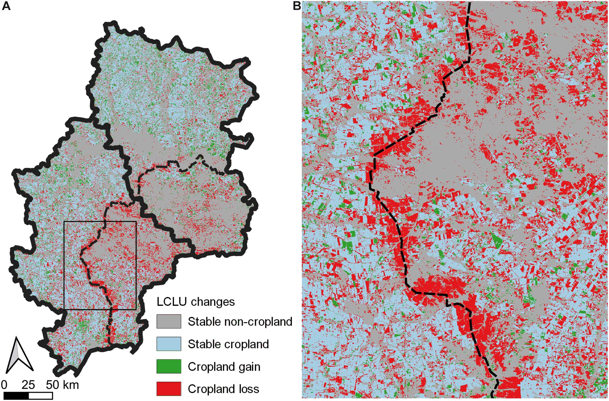
Figure 3. Changes in cropland areas in the Donetsk and Luhansk regions. Cropland changes in 2013 and 2018 (A). Subset of panel (A) (identified by a rectangle) (B). Cropland losses were not uniform throughout the region with most of losses happening along the border line and in the areas controlled by militants. The majority of cropland losses were due to abandonment, showing a return to natural vegetation.

FIGURE 4

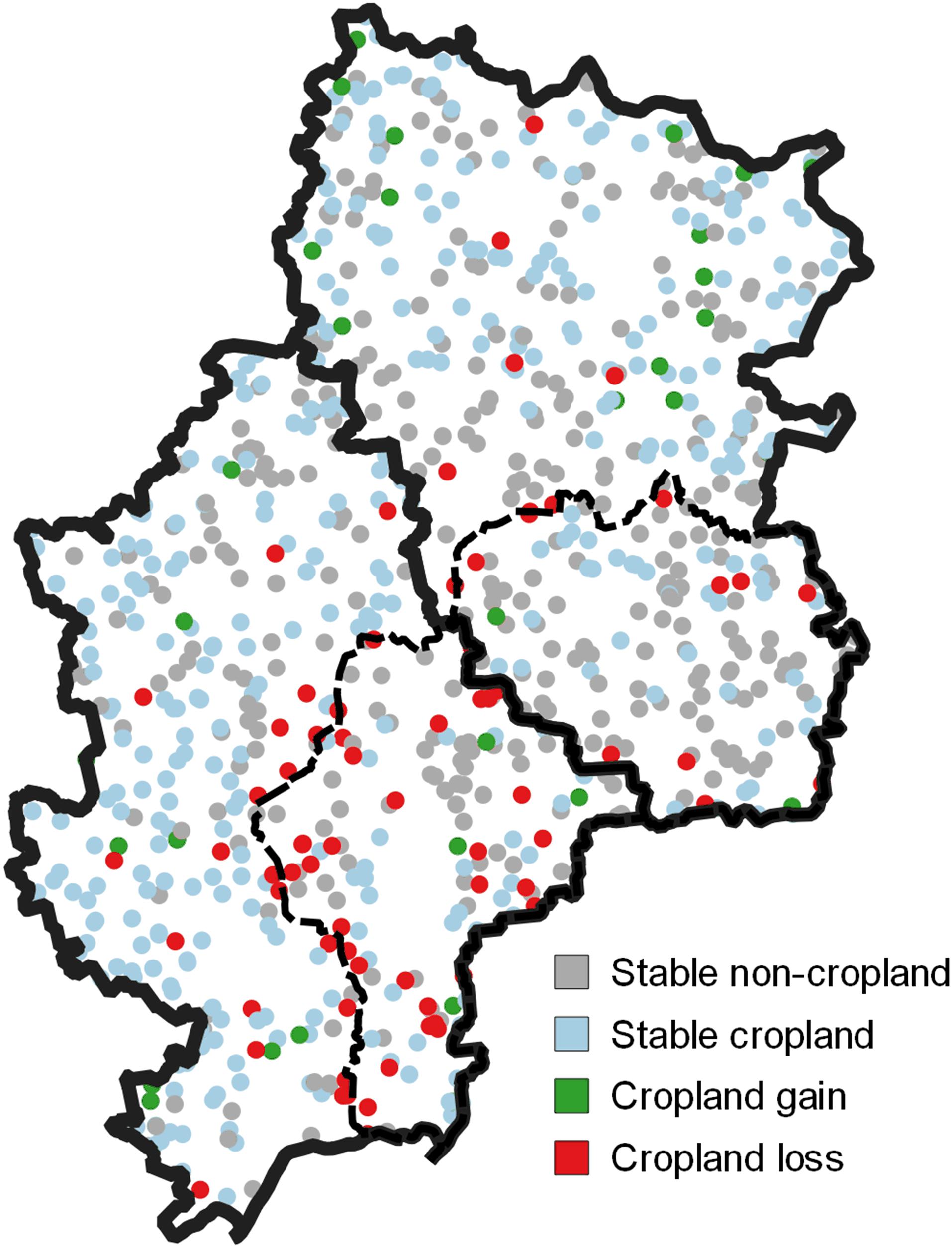
Figure 4. Location of 831 reference samples, which were used to estimate areas of cropland changes. The distribution of samples among four strata was as follows: 308 samples for strata “Stable non-cropland,” 220 samples for “Stable cropland,” 126 samples for “Cropland gain,” and 177 samples for “Cropland loss.”

Overall Cropland Area Changes

In 2013, cropland accounted for 1.46 ± 0.04 Mha and 1.11 ± 0.03 Mha of the Donetsk and Luhansk regions, respectively. The uncertainty is represented as ± 1 standard error (SE) of the estimate. These values represent a 2.2 and 8.0% overestimation compared to the official statistics provided by the SSSU. Typically, cropland area is underestimated by the official statistics due to imperfect data collection protocols and under-reporting by crop producers (Gallego et al., 2014; Kussul et al., 2017a). For 2018, our satellite-based estimates were cropland losses for the entire region of 188.8 ± 19.2 Tha for Donetsk and 64.2 ± 12.7 Tha for Luhansk regions, while cropland gains were 53.5 ± 13.2 Tha for Donetsk and 63.0 ± 14.0 Tha for Luhansk. Net cropland losses (loss minus gains) were 135.3 ± 23.3 Tha (p-value = 8 × 10^–8) and 1.2 ± 18.9 Tha (p-value = 0.95) in Donetsk and Luhansk regions, respectively. The identified cropland gains were due to transitions from fallow. For the Donetsk region, net cropland losses accounted for 9.2% of the cropland area in 2013. For Luhansk region, cropland gains and losses were offset.

Cropland Area Changes in the Areas Under (and Not Under) Control of the Ukrainian Government

In the areas under the control of the Ukrainian Government (Figure 2), we observed cropland net losses 39.8 ± 15.6 Tha (p-value = 0.011) for Donetsk and cropland net gains 31.2 ± 16.1 Tha (p-value = 0.054) for Luhansk. Those cropland gains were primarily due to conversion from fallow to cropland (100% in Donetsk and 94% in Luhansk). However, the derived uncertainties were too high to make any conclusions on cropland gains/losses. However, different patterns were observed in the partially occupied areas. In the areas not under control of the Ukrainian Government, net cropland losses were 97.5 ± 17.6 Tha (p-value = 2 × 10^–7) in Donetsk and 31.4 ± 10.2 Tha (p-value = 0.0025) in Luhansk. These estimates account for 25.7 and 14.8% loss of cropland areas (since 2013) in those sub-regions of Donetsk (379.9 ± 24.2 Tha) and Luhansk (212.0 ± 14.1 Tha) regions, respectively. The majority of cropland losses were due to abandonment, showing a return to natural vegetation: 60% in Donetsk and 73% in Luhansk regions. Cropland gains were not substantial (6.1% in Donetsk and 3.0% in Luhansk) and were due to transition from fallow. The losses in cropland areas would lead to reduction in crop production. Assuming contribution of agriculture to regional GVA at 7.6% in Donetsk region (average 2014–2017) and 18.6% in Luhansk region (Figure 1), that would account 2.0 and 2.8% reduction in GVA for Donetsk and Luhansk regions, respectively.

Cropland Area Changes Within the Border Line

We also estimated cropland areas within a ± 7 km buffer zone along the conflict border line, which is subject to active combat operations. The net cropland losses were estimated at 93.5 ± 12.7 Tha (p-value = 1 × 10^–15), which constitutes 46% of the cropland area estimates in 2013 for this zone. Those cropland losses were due to abandonment and a return to natural vegetation (88%).

Discussion and Conclusion

The military conflict in Southeast Ukraine has been continuing since 2014, and the present study highlighted regional LCLU changes associated with this conflict. We found that cropland losses were not uniform throughout Donetsk and Luhansk regions, but were substantial in the areas controlled by militants and within the border area, where combat activities occur. In those regions, up to 46% cropland areas were abandoned relative to the 2013 cropland estimates and are returning to natural vegetation. These results highlight the utility of spatially explicit information acquired from Earth observation satellites, especially for areas, where collecting ground-based data is impractical. While the present study provides a snapshot of changes occurred during 2013–2018 period, further work is needed to monitor and quantify long-term consequences of the conflict on the environment in the Southeastern Ukraine.

Data Availability Statement

Maps and reference data are available at ftp://ftp.iluci.org/Sergii/ukraine-cropland-change.

Author Contributions

SS, CJ, NK, and AS designed the research. SS and ML performed the research. SS, NK, AS, and ML analyzed and interpreted the data. SS and CJ wrote the manuscript.

Funding

This work was supported by the NASA Land-Cover and Land-Use Change (LCLUC) Program, grant no. 80NSSC18K0336 and NASA Harvest Consortium (NASA Applied Sciences), grant no. 80NSSC17K0625.

Conflict of Interest

The authors declare that the research was conducted in the absence of any commercial or financial relationships that could be construed as a potential conflict of interest.

Supplementary Material

The Supplementary Material for this article can be found online at: https://www.frontiersin.org/articles/10.3389/feart.2019.00305/full#supplementary-material

References

Arvidson, T., Gasch, J., and Goward, S. N. (2001). Landsat 7’s long-term acquisition plan—an innovative approach to building a global imagery archive. Remote Sens. Environ. 78, 13–26. doi: 10.1016/s0034-4257(01)00263-2

CrossRef Full Text | Google Scholar

Claverie, M., Ju, J., Masek, J. G., Dungan, J. L., Vermote, E. F., Roger, J.-C., et al. (2018). The harmonized Landsat and Sentinel-2 surface reflectance data set. Remote Sens. Environ. 219, 145–161. doi: 10.1016/j.rse.2018.09.002

CrossRef Full Text | Google Scholar

Davis, C. M. (2016). The Ukraine conflict, economic–military power balances and economic sanctions. Postcommunist Econ. 28, 167–198. doi: 10.1080/14631377.2016.1139301

CrossRef Full Text | Google Scholar

Drusch, M., Del Bello, U., Carlier, S., Colin, O., Fernandez, V., Gascon, F., et al. (2012). Sentinel-2: ESA’s optical high-resolution mission for GMES operational services. Remote Sens. Environ. 120, 25–36. doi: 10.1016/j.rse.2011.11.026

CrossRef Full Text | Google Scholar

Farr, T. G., Rosen, P. A., Caro, E., Crippen, R., Duren, R., Hensley, S., et al. (2007). The shuttle radar topography mission. Rev. Geophys. 45:RG2004.

Google Scholar

Gallego, F. J., Kussul, N., Skakun, S., Kravchenko, O., Shelestov, A., and Kussul, O. (2014). Efficiency assessment of using satellite data for crop area estimation in Ukraine. Int. J. Appl. Earth Obs. Geoinf. 29, 22–30. doi: 10.1016/j.jag.2013.12.013

CrossRef Full Text | Google Scholar

Gutman, G., and Radeloff, V. (2016). Land-Cover and Land-Use Changes in Eastern Europe After the Collapse of the Soviet Union in 1991. Switzerland: Springer.

Google Scholar

Holben, B. N. (1986). Characteristics of maximum-value composite images from temporal AVHRR data. Int. J. Remote Sens. 7, 1417–1434. doi: 10.1080/01431168608948945

CrossRef Full Text | Google Scholar

Ivanov, O. (2015). Social background of the military conflict in ukraine: regional cleavages and geopolitical orientations. Soc. Health Commun. Stud. J. 2, 52–73.

Google Scholar

Kussul, N., Kolotii, A., Adamenko, T., Yailymov, B., Shelestov, A., and Lavreniuk, M. (2017a). “Ukrainian cropland through decades: 1990–2016,” in Proceedings of the 2017 IEEE First Ukraine Conference on Electrical and Computer Engineering — UKRCON, Kyiv, 856–860.

Google Scholar

Kussul, N., Lavreniuk, M., Skakun, S., and Shelestov, A. (2017b). Deep learning classification of land cover and crop types using remote sensing data. IEEE Geosci. Remote Sens. Lett. 14, 778–782. doi: 10.1109/lgrs.2017.2681128

CrossRef Full Text | Google Scholar

Lesiv, M., Schepaschenko, D., Moltchanova, E., Bun, R., Dürauer, M., Prishchepov, A. V., et al. (2018). Spatial distribution of arable and abandoned land across former soviet union countries. Sci. Data 5:180056. doi: 10.1038/sdata.2018.56

PubMed Abstract | CrossRef Full Text | Google Scholar

Li, J., and Roy, D. (2017). A global analysis of sentinel-2A, Sentinel-2B and Landsat-8 Data Revisit Intervals and Implications for Terrestrial Monitoring. Remote Sens. 9:902. doi: 10.1016/j.scitotenv.2017.08.219

PubMed Abstract | CrossRef Full Text | Google Scholar

Nair, V., and Hinton, G. E. (2010). “Rectified linear units improve restricted Boltzmann machines,” in Proceedings of the 27th International Conference on Machine Learning — ICML-10, eds J. Fürnkranz, and T. Joachims, (Haifa: Omnipress), 807–814.

Google Scholar

Olofsson, P., Foody, G. M., Herold, M., Stehman, S. V., Woodcock, C. E., and Wulder, M. A. (2014). Good practices for estimating area and assessing accuracy of land change. Remote Sens. Environ. 148, 42–57. doi: 10.1016/j.rse.2014.02.015

CrossRef Full Text | Google Scholar

Phillips, D. L. (1962). A technique for the numerical solution of certain integral equations of the first kind. J. Assoc. Comput. Machinery 9, 84–97. doi: 10.1145/321105.321114

CrossRef Full Text | Google Scholar

Roy, D. P., Wulder, M. A., Loveland, T. R., Woodcock, C. E., Allen, R. G., Anderson, M. C., et al. (2014). Landsat-8: science and product vision for terrestrial global change research. Remote Sens. Environ. 145, 154–172.

Google Scholar

Skakun, S., Kussul, N., Shelestov, A. Y., Lavreniuk, M., and Kussul, O. (2015). Efficiency assessment of multitemporal C-band Radarsat-2 intensity and Landsat-8 surface reflectance satellite imagery for crop classification in Ukraine. IEEE J. Sel. Top. Appl. Earth Obs. Remote Sens. 9, 3712–3719. doi: 10.1109/jstars.2015.2454297

CrossRef Full Text | Google Scholar

Smaliychuk, A., Müller, D., Prishchepov, A. V., Levers, C., Kruhlov, I., and Kuemmerle, T. (2016). Recultivation of abandoned agricultural lands in Ukraine: patterns and drivers. Glob. Environ. Change 38, 70–81. doi: 10.1016/j.gloenvcha.2016.02.009

CrossRef Full Text | Google Scholar

Stehman, S. V. (2013). Estimating area from an accuracy assessment error matrix. Remote Sens. Environ. 132, 202–211. doi: 10.1186/s13021-017-0075-z

PubMed Abstract | CrossRef Full Text | Google Scholar

Tikhonov, A. N., Leonov, A. S., and Yagola, A. G. (1998). Nonlinear Ill-Posed Problems. London: Chapman & Hall.

Google Scholar

Vasylyeva, T. I., Liulchuk, M., Friedman, S. R., Sazonova, I., Faria, N. R., Katzourakis, A., et al. (2018). Molecular epidemiology reveals the role of war in the spread of HIV in Ukraine. Proc. Natl. Acad. Sci. U.S.A. 115, 1051–1056. doi: 10.1073/pnas.1701447115

PubMed Abstract | CrossRef Full Text | Google Scholar

Waldner, F., De Abelleyra, D., Verón, S. R., Zhang, M., Wu, B., Plotnikov, D., et al. (2016). Towards a set of agrosystem-specific cropland mapping methods to address the global cropland diversity. Int. J. Remote Sens. 37, 3196–3231. doi: 10.1080/01431161.2016.1194545

CrossRef Full Text | Google Scholar

Woroniecka-Krzyzanowska, D., and Palaguta, N. (2016). Internally displaced persons and elections under military conflict in Ukraine. J. Refug. Stud. 30, 27–46.

Google Scholar