Mapping Snowmelt Progression in the Upper Indus Basin With Synthetic Aperture Radar
 Jewell Lund1*
  Richard R. Forster1
  Summer B. Rupper1
  Elias J. Deeb2
  H. P. Marshall3
  Muhammad Zia Hashmi4
  Evan Burgess1
- 1Snow and Ice Research Lab, Department of Geography, University of Utah, Salt Lake City, UT, United States
- 2Cold Regions Research Engineering Laboratory, US Army Corps of Engineers, Hanover, NH, United States
- 3Cryosphere Geophysics and Remote Sensing Group, Department of Geosciences, Boise State University, Boise, ID, United States
- 4Water Resources and Glaciology Section, Global Change Impact Studies Centre, Islamabad, Pakistan
The Indus River is a vital resource for food security, ecosystem services, hydropower, and economy for millions of people living in Pakistan, India, China, and Afghanistan. Glacier and snowmelt from the high altitude Himalaya, Karakoram, and Hindu Kush mountain ranges are the largest drivers of discharge in the upper Indus Basin (UIB), and contribute significantly to Indus flows. Complex climatology and topography, coupled with the challenges of field study and meteorological measurement in these rugged ranges, elicit notable uncertainties in predicting seasonal runoff as well as cryospheric response to changes in climate. Here we utilize Sentinel-1 synthetic aperture radar (SAR) imagery to track ablation season development of wet snow in the Shigar Watershed of the Karakoram Mountains in Pakistan from 2015 to 2018. We exploit opportune local image acquisition times to highlight diurnal differences in radar indications of wet snow, and examine the spatial and temporal contexts of radar diurnal differences for 2015, 2017, and 2018 ablation seasons. Radar classifications for each ablation season show spatial and temporal patterns that indicate a dry winter snowpack undergoing diurnal surface melt-refreeze cycles, transitioning to surface snow that remains wet both day and night, and finally snow free conditions following melt out. Diurnally differing SAR signals may offer insights into important snowpack energy balance processes that precede melt out, which could provide useful constraints for both glacier mass balance modeling and runoff forecasting in remote alpine watersheds.
Introduction
Snow and ice play critical roles worldwide in water resources and climate. An estimated 75% of fresh water resources are stored in ice sheets and glaciers (Meier and Post, 1995). About 1.2 billion people rely on snowmelt for agriculture and consumption (Barnett et al., 2005). At its peak, 57 million square kilometers of northern hemisphere land are covered in snow each season, and over 15 million square kilometers receive 40% or more of total annual precipitation as snowfall (Déry and Brown, 2007). Seasonal and perennial snowpacks and glaciers act as natural reservoirs, providing runoff during the hottest months of the year, and in complementary timeframes. In addition to direct runoff resources, snow and ice play a critical role in climate: significant portions of incident solar radiation are reflected away from the earth surface due to the high albedo of snow and ice, resulting in a cooling effect critical to the surface energy budget. The role of snowmelt in primary production and ecosystems services is important and unique to each area (Vaughan et al., 2013). The most recent IPCC (Core Writing Team et al., 2014) reports a continued shrinkage of worldwide glacier mass balance, as well as a decrease in northern hemisphere snow cover extent, both reported at very high confidence.
Of the major Asian river basins, the Indus relies most heavily on snow and glacial melt (Immerzeel et al., 2010), primarily from the upstream Karakoram, Hindu Kush, and Himalayan mountain ranges (Figure 1). The majority of flows in the upper Indus Basin (UIB) derive from glacier and snowmelt, which are estimated to contribute 65–85% of annual flows (Hewitt et al., 1989; Wake, 1989; Archer and Fowler, 2004; Immerzeel et al., 2009; Tahir et al., 2011; Mukhopadhyay and Khan, 2015; Shrestha et al., 2015). An arid regional climate necessitates direct reliance on these flows for food security, economy, and hydroelectric power for millions of people living in the Indus River Basin (Immerzeel and Bierkens, 2012; Hasson et al., 2014; Immerzeel et al., 2015). As the Indus River Basin incorporates portions of China, India, Afghanistan, and Pakistan, this reliance also strongly impacts international relations (Wescoat et al., 2000; Wheeler, 2011).
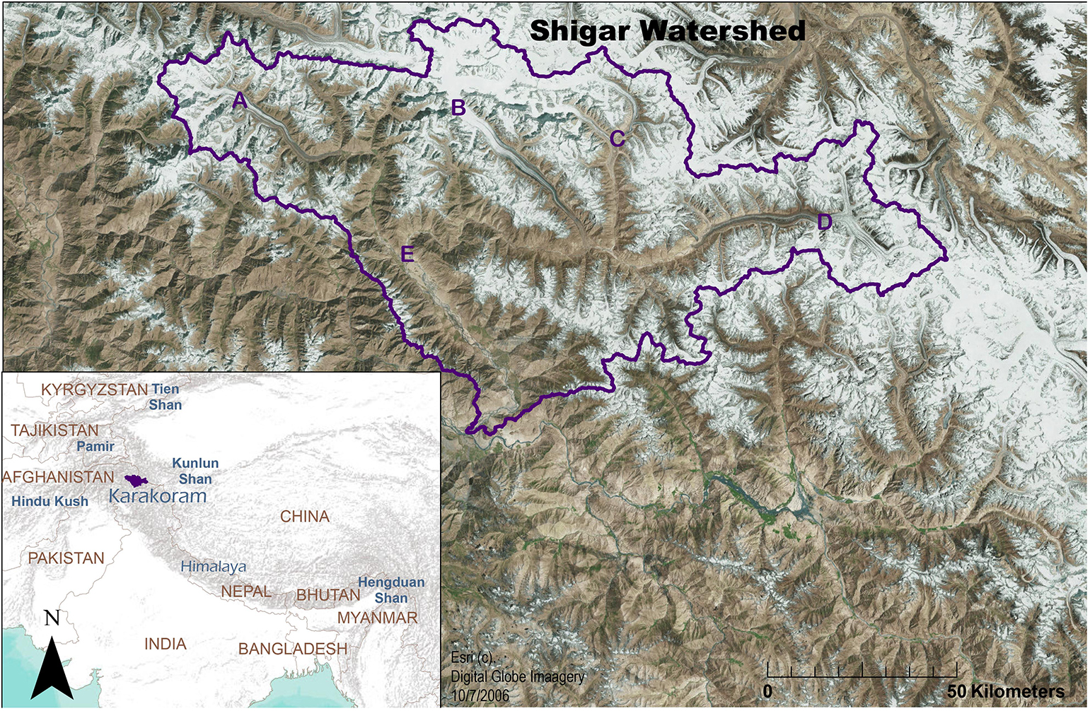
Figure 1. Major ranges in High Mountain Asia (HMA). Highlighted is the Shigar Watershed, located in the Karakoram Mountains. (A) Chogo Lungma glacier. (B) Biafo Glacier. (C) Choktoi and Panmah Glaciers. (D) Baltoro Glacier. (E) Shigar WAPDA DCP meteorological station approximate location.
The Karakoram Mountains, located in the far northwest of the Himalayan arc, contribute to flows of the UIB with nearly 8,000 glaciers that span an area of 18,000 km2, ranging in altitude from 2300 to 8600 m.a.s.l (RGI Consortium, 2017). More than 90% of the total area can be snow covered seasonally, and perennial snow cover is significant (Hewitt et al., 1989; Immerzeel et al., 2009; Hasson et al., 2014).
The Karakoram stand at the nexus of large-scale atmospheric circulation systems, the interaction of which directly impact snowpack and glaciers in the region. Mediterranean Westerly flows deliver the bulk of annual precipitation in the winter months, although the South Asian Monsoon can also penetrate the range in summer months, providing a portion of yearly precipitation (Hewitt et al., 1989; Wake, 1989; Winiger et al., 2005; Maussion et al., 2014). Forsythe et al. (2017) have identified the interplay of these two major atmospheric circulation systems as the primary climatic driver of declining summer temperatures – and thus reduced glacial ablation – in the Karakoram region for the latter part of the 20th century. Forsythe et al. (2017) note both that the “Karakoram Anomaly” (or summer temperature reduction) has been weakening in the first part of the 21st century, and also that the impact of climate change on large-scale atmospheric circulation patterns remains an open question. This dynamic interplay, coupled with the paucity of meteorological measurements in high altitude catchments, perhaps explain the large number of studies with contradictory conclusions for climatic trends in the Karakoram including precipitation, temperature, snow covered area, and streamflow (Archer and Fowler, 2004; Hewitt, 2005, 2011; Winiger et al., 2005; Fowler and Archer, 2006; Immerzeel et al., 2009; Chen et al., 2010; Bocchiola et al., 2011; Tahir et al., 2011, 2015, 2016; Kapnick et al., 2014; Mukhopadhyay and Khan, 2014; Kääb et al., 2015; Reggiani et al., 2016).
Considering the challenges of field study and climatic complexity in the region, utilizing remote sensing techniques that offer information on differing electromagnetic, spatial, and temporal scales can provide useful information on the status of snow and ice. Digital elevation model (DEM) difference techniques offer critical and high spatial-resolution insight into glaciological change, but limit knowledge of variability in between image timestamps and do not provide direct evidence of the mechanism(s) responsible for any changes. Daily optical datasets such as MODIS snow cover area offer temporally useful information, but at spatial resolutions (typically 500 m) that limit insight into many important snowpack processes. MODIS snow cover products, often used for snowmelt runoff modeling, have been found to perform less accurately in High Mountain Asia (HMA) compared to North American mountain ranges, likely due to steep topography (Rittger et al., 2013). Cloud cover continues to pose a significant challenge in utilizing optical imagery for identifying snow cover, and can result in missing data and misclassified pixels (Parajka and Blöschl, 2008).
The European Space Agency’s (ESA) Sentinel-1 (S1) C-band synthetic aperture radar (SAR) sensor provides publicly available imagery with an overpass repeat of approximately 12 days. SAR images are acquired regardless of cloud cover or sun illumination, at a spatial resolution on the order of tens of meters. Because of backscatter sensitivity to surface roughness and dielectric properties, radar offers unique insight to surface states that may elucidate energy balance conditions for the snowpack prior to seasonal melt out (Mätzler and Hüppi, 1989; Cogley, 2011; Ragettli et al., 2013). In this study, we utilize S1 SAR imagery in the heavily glaciated Shigar Watershed of the Karakoram Mountains to examine seasonal and diurnal snowpack conditions through multiple ablations seasons. We compare SAR-derived snow conditions maps with optically-derived snow cover maps, and track inter-annual variability in radar snowmelt conditions. When acquisition patterns allow, we also identify diurnal changes in radar indications of snowmelt. We quantify the diurnal differences (contrast between night and day) in radar signals, and explore their spatial and temporal context throughout the melt seasons of 2015, 2017, and 2018.
Synthetic aperture radar indications of snowpack conditions can offer critical insight into energy balance processes on a subseasonal timescale, in an area with limited field measurement and variable cryospheric responses to climate. This information could be integrated into both glacier mass balance modeling as well as runoff forecasting, which could improve with physically based parameterizations and multivariate calibration to understand the current drivers of cryospheric change.
Background
To understand the potential, limitations, and implications of radar interpretation of snowpack conditions, we first discuss snowpack energy fluxes and in particular the processes that dominate the seasonal transition prior to runoff. Next, we examine the impact of snowpack conditions on radar backscatter.
Snowpack Energy Balance
Seasonal Transitions: A Melting Snowpack
The transition of a cold winter snowpack to an isothermal (or ripe) snowpack at the melting point is the result of complex processes of energy transfer at the boundaries of and within the snowpack (DeWalle and Rango, 2008). Understanding this transition is crucial for energy balance modeling and runoff forecasting for snow and ice; however, its onset and duration can vary substantially from year to year (Kattelmann and Dozier, 1999). This transition can be understood in three general phases: (1) warming, (2) ripening, and (3) runoff. Energy for all three of these phases is dominated at the surface by net solar radiation, which is determined by irradiance and snow albedo (Oerlemans, 2000; Bales et al., 2006; Painter et al., 2007, 2012). Once the snow surface warms to 0°C and excess energy generates melt, liquid water dominates mass and energy exchange within the snowpack (Colbeck, 1976; Pfeffer et al., 1990; Sturm et al., 1997; Macelloni et al., 2005; DeWalle and Rango, 2008; Cuffey and Paterson, 2010; Painter et al., 2012).
Diurnal Fluctuations in Energy Balance
As shortwave radiation is a dominant source of melt energy during daylight hours (DeWalle and Rango, 2008), nighttime radiative fluxes consequently contrast strongly to those during the day. Liquid water held by capillary forces in the snowpack can refreeze overnight due to a negative energy flux to the atmosphere, often dominated by longwave and sensible heat fluxes from a melting snowpack constrained to 0°C. At the surface, refrozen crusts can develop quickly and become quite thick overnight (Mätzler and Hüppi, 1989; Macelloni et al., 2005). Early in the ablation season, the entire depth of liquid water within the snowpack can refreeze overnight (Mätzler and Hüppi, 1989). Later in the season, the bulk of the snowpack more often remains wet with a thin layer of refreeze just at the surface, typically in the first 10 centimeters; in this case, the snowpack remains ripe but the refrozen crust presents an energy deficit that must be overcome before melt can resume the next day (Macelloni et al., 2005; Samimi and Marshall, 2017). The “recycling” of melt water due to nightly refreeze can act as a significant energy sink. For example, Samimi and Marshall (2017) concluded that 10–15% of available melt energy for a given season was diverted to warm and melt refrozen meltwater on the Haig Glacier in Canada.
Synthetic Aperture Radar
Radar and the Snowpack
Radar interaction at microwave wavelengths with the snowpack takes place at three different boundaries: the air-snow interface, within the snowpack, and the snow-substrate interface. In dry snow, C-band radar (centered at 5 cm wavelength) penetration depth varies from 5–20 m (Mätzler, 1987; Rignot et al., 2001; Langley et al., 2007). The primary source of backscatter and reflection stems from radar interaction at the snow-ground or snow-ice interface, although refrozen features in the snowpack can also contribute volumetric scattering (Mätzler, 1987).
With liquid water present in the snowpack, microwave interaction changes drastically, primarily because of the order of magnitude difference in permittivity of liquid water compared to ice or air. In a 0.3 m thick snowpack with 1% liquid water content by volume (likely less than irreducible water content), Nagler (1996) found C-band radar penetration limited to 0.11 m, approximately two wavelengths. In snow with liquid water content of 5% by volume, radar penetration is typically limited to a singular wavelength, resulting in extremely low backscatter (Mätzler, 1987; Martinec and Rango, 1991; Techel and Pielmeier, 2011). With increasing water content, backscatter values from the snowpack decrease, providing the basis for threshold-based wet snow identification (Mätzler, 1987; Ulaby et al., 2014). Developed as a means to circumnavigate topographic effects on backscatter values, the threshold-based comparison is possible because backscatter values from similar SAR geometries of snow-free or dry-snow covered surfaces vary little over time, compared to the strongly attenuated backscatter of snow with liquid water present (Nagler, 1996). In this case, the actual backscatter value – which may be influenced by local incidence angle – is less important than the relative change in backscatter values over time. Threshold-based wet snow identification is derived from the ratio between a melt season image and a reference image from the same orbital track (and thus nearly identical SAR imaging geometry). Ideally, the reference image is an average of several images during dry snow or snow free conditions, reducing potential small inter-image variations. Based on field study and comparison with optical data, threshold ranges from −2 to −3 dB have been shown to consistently identify wet snow in alpine areas using co-polarized SAR data; a threshold of −3 dB is most commonly used (Nagler, 1996; Nagler and Rott, 1998, 2000; Floricioiu and Rott, 2001; Valenti et al., 2008; Nagler et al., 2016).
Radar-based wet snow identification is only indicative of liquid water in the uppermost centimeters of the layer in which it is identified. Because of the significant attenuation in C-band radar, the presence or absence of liquid water in the snowpack underneath this layer likely does not affect backscatter values. The time difference between first surface wetting and snowpack ripening can vary from hours to weeks, and is a significant challenge in runoff forecasting that cannot be resolved by remote sensing data alone (Kattelmann and Dozier, 1999; Heilig et al., 2015). However, the clear identification of liquid water in the snowpack possible with radar offers an important indicator of seasonal transitions in snowpack energy balance, as well as spatially explicit information of areas of the snowpack that could potentially contribute to runoff.
Diurnal Changes in Radar Return
Several studies of microwave signatures in alpine snowpacks have observed temporal variations of backscatter in wet snowpacks due to surface refreezing, which causes an increase in backscatter due to the high volumetric scattering of the large grains of the refrozen layer (Brun, 1989; Floricioiu and Rott, 2001; Nagler et al., 2016; Reber et al., 1987; Strozzi et al., 1997). A paucity of SAR sensors with consistent acquisition patterns has limited ongoing research of spaceborne backscatter signals from refrozen snow surfaces and their seasonal evolution. However, Strozzi et al. (1997) observed backscatter changes in sensors at varying frequencies for melt-freeze crusts in the Austrian Alps. While higher frequency wavelengths were better able to identify refrozen crusts stratigraphically over either wet or dry snow, C-band radar could reliably detect refrozen crusts over a dry snowpack, e.g., early melt season diurnal cycles that refreeze the entirety of melt water in a snowpack that is not yet ripe (Mätzler and Hüppi, 1989; Fahnestock et al., 1993; Nagler, 1996; Strozzi et al., 1997).
Study Area, Data, and Methods
Shigar Watershed
The Shigar Watershed (Figure 1) is located in the central Karakoram Mountains, with an altitude spanning about 2100 m to over 8600 m. The watershed area is approximately 7000 km2, about 30% of which is glaciated (Pfeffer et al., 2014). Though one of the smaller watersheds of the UIB, the Shigar contributes significantly to total UIB flows – about 8% of annual flows, and 10–11% of the flows during July, August, and September (Mukhopadhyay and Khan, 2014). Flow analysis by Mukhopadhyay and Khan (2014) led them to conclude that mid-altitude snowmelt from the Shigar peaks in June, while high altitude source-flows show two distinct peaks: in July, which they posit originates from snow melt, and also in August originating from glacial melt. In their study, Mukhopadhyay and Khan (2015) calculated snow and glacier melt to contribute 43% and 35% of total runoff for the Shigar basin, respectively. An analysis of snow cover by Hasson et al. (2014) using MODIS products from 2001 to 2012 concludes that the Shigar holds the highest annual snow cover percentage of the UIB sub-basins, averaging 90 ± 3% of the total area at maximum and a minimum coverage of 25 ± 8%. Snow cover trends from 2001 to 2012 for the Shigar were not statistically significant, but nevertheless showed a decrease in the winter and autumn months, and an increase in spring and summer months. The glaciers of the central Karakoram have been reported in near-balance, albeit with significant spatial and temporal heterogeneity, including surge-type glaciers (Gardelle et al., 2012b; Brun et al., 2017; Lin et al., 2017; Zhou et al., 2017).
Data
Sentinel-1 SAR Imagery
Radar imagery is collected from the ESA S1 constellation, operating at a center frequency of 5.407 GHz (C-band) with single look complex (SLC) images in 5 m by 20 m spatial resolution in range and azimuth directions, respectively. The first S1 satellite launched in April of 2014; after a ramp-up and exploitation phase, and along with the launch of Sentinel-1 B in April 2016, the S1 observation scenario now consistently offers a revisit frequency in the Karakoram region of 12 days for ascending and descending passes in dual polarization (VV and VH). Of significance for our study of the Shigar Watershed is the timing of acquisition: 2015, 2017, and 2018 acquisitions regularly consisted of an ascending pass at approximately 18:00 local time, followed by a descending pass the next morning at 6:00 local time. As the minimum daily snowpack liquid water content has been found to occur in early hours of the morning (e.g., Kattelmann and Dozier, 1999), these acquisition times are opportune to examine diurnal differences in radar indications of snow conditions. It is worth noting that, at C-band, cross-polarized wavelengths distinguish wet snow at low incidence angles more accurately than co-polarized (Nagler et al., 2016). However, S1 dual polarization images are only consistently available starting with the 2017 melt season; in order to compare multiple ablation seasons, only co-polarized (VV) images are utilized in this study.
European Space Agency’s S1 imagery was downloaded through the Alaska Satellite Facility Distributed Active Archive Center (Copernicus a). Singular ascending and descending S1 tracks were selected that cover the entire Shigar Watershed, and every available image downloaded from October 2014 through October 2018 in SLC format. From these images, at least three winter reference dates were selected for each year, as well as images throughout the 2015–2018 ablation seasons (approximately April through October) along matching orbital tracks (Supplementary Table S1).
SRTM 1 Arc-Second Digital Elevation Model
The shuttle radar topography mission (SRTM) 1 arc-second global DEM, void filled and openly distributed through the US Geological Survey (USGS) at a resolution of 30 meters, was used for processing and analysis (USGS). Though SRTM operated at C-band wavelength, which has been estimated to penetrate Karakoram ice by an average of 2.7–3.0 m (Gardelle et al., 2012a; Zhou et al., 2017), it showed fewer artifacts in comparison to other available DEMs for the region with comparable spatial resolution [e.g., advanced spaceborne thermal emission and reflection radiometer (ASTER) global digital elevation map (GDEM)]. As we are interested in the relative elevation change of wet snow (which will limit radar penetration to a few centimeters) overlying either ice or ground, we assume ice penetration to be an irrelevant issue in this study.
Sentinel-2 Level 2A Snow and Cloud Confidence Maps
We compare SAR-derived snow conditions maps to snow cover maps from Level 2A Sentinel-2 (S2) snow and cloud confidence products. ESA’s S2 is a high spatial resolution optical sensor with a repeat time of 5 days, utilizing two sensors with sun-synchronous orbits. 13 spectral bands offer reflectance measurements at three different spatial resolutions (10–60 m). Level 1C (top-of-atmosphere reflectance) products were downloaded from the USGS and processed into Level-2A products (Copernicus b, USGS). Level-2A products, which denote atmospherically corrected reflectance, include both snow and cloud confidence maps. The snow confidence map is derived from a four-step filtering process utilizing the Normalized Difference Snow Index (Hall and Riggs, 2010) as well as thresholds on bands 2, 4, 8, and 11. The output of the snow confidence map also feeds into the cloud confidence map, a seven-step filter utilizing NDSI and Normalized Difference Vegetation Index thresholds, as well as ratios from bands 2, 3, 8, and 11 to minimize misclassification with soils and water, rock and sand, and senescing vegetation (Richter et al., 2012).
Meteorological Data
Daily temperature readings at the Pakistan Water and Power Development Authority (WAPDA) Shigar data collection platform (DCP), located at 2367 m.a.s.l (Figure 1) are compared to SAR-derived snow conditions for the 2015 ablation season. These data are generously provided by the WAPDA Glacier Monitoring and Research Center (GMRC) through correspondence with Pakistan’s Global Change Impact Studies Centre (GCISC).
HMA ASCAT Freeze/Thaw/Melt Status
S1 wet snow maps are compared with daily freeze/melt status over the Shigar Watershed from the NSIDC HMA ASCAT Freeze/Thaw/Melt Status dataset (Steiner and McDonald, 2018). Derived from C-band backscatter measurements from the Advanced Scatterometer (ASCAT) on EUMETSAT Metop-A and Metop-B satellites, images are spatially enhanced using the Scatterometer Image Reconstruction algorithm (Early and Long, 2001), and 3-day composites of ascending morning acquisitions are interpolated to create a daily product at approximately 4.45 km spatial resolution. This product is available from January 1, 2009 through October 12, 2017.
Methods
S1 Image Processing
The SAR image processing and postprocessing workflows for each melt season image can be viewed in Figure 2. After applying precise orbit information, each interferometric wideswath (IW) image is “deburst” and radiometrically calibrated to beta nought, or radar brightness, in preparation for terrain-flattening (Small, 2011). After calibration, multi-looking (spatial averaging) is performed; eight looks in the range and two looks in the azimuth direction result in pixels with approximately 30 m resolution in both directions. In order to minimize terrain effects on backscatter, radiometric terrain flattening is then performed according to the methodology developed by Small (2011), utilizing the SRTM 1 Arc-Second DEM. Radiometric terrain flattening spatially integrates brightness values (in original radar geometry) through a reference DEM to determine a specific illuminated area according to each radar position, which is then used for reference area normalization, resulting in a quantity referred to as gamma nought. Small’s method provides a more robust incorporation of local topography in SAR processing, and potentiates cross-track and even cross-sensor comparisons, which have previously been challenged due to varying SAR acquisition geometries especially in regions of high relief.
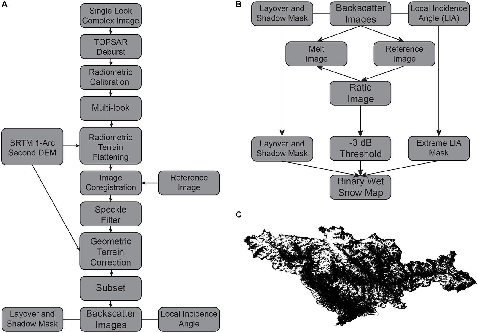
Figure 2. (A) SAR processing and (B) post processing workflows, the product of which is a (C) binary wet snow map. White pixels indicate wet snow. Processing was accomplished with ESA open source SNAP software; postprocessing accomplished through R.
Melt season images are co-registered with a reference image, which is an average of at least three images from the previous winter. Due to S1 instrument stability and precise orbital information, sub-pixel co-registration is achieved. After co-registration, speckle filtering is performed using the Refined Lee filter (Lee, 1981). Lastly, geometric terrain correction is accomplished through bilinear interpolation re-sampling with the SRTM DEM, resulting in images with a final pixel spacing of 29.02 m. As a final step in processing, images are subset to Shigar Watershed boundaries. Along with geometrically terrain-corrected gamma nought values, layover and shadow information, as well as local incidence angle calculations are collected for each image. Images are processed with the Sentinel-1 Toolbox within the open-source Sentinel Application Platform (SNAP–ESA).
S1 Postprocessing
Following image processing, a ratio image is generated by comparing backscatter values of the melt image to the co-registered reference winter image. Pixels with a ratio value at or less than −3 dB (Nagler, 1996) are designated as “wet snow,” resulting in a binary wet snow map, visible in Figure 2C. Noting that more recent studies of threshold-based wet snow mapping select a threshold of −2 dB (e.g., Nagler et al., 2016), we test different threshold values within a range of −2 and −3 dB on an image from May 23–24, 2015. This image is selected as it has appreciable areas of pixels classified as both wet and dry, as well as a notable amount of pixels that change classification overnight (refer to Figure 9). Along with the ratio image, a mask is generated for each date that excludes pixels in layover or shadow, as well as extreme local incidence angles. While radiometric terrain flattening significantly improves radiometric accuracy, we find backscatter values are still impacted by extreme incidence angles. Thus, we adopt a conservative approach as in Nagler et al. (2016) and mask out any pixels with local incidence angles less than 15 or greater than 75 degrees.
Pixel Classification
Once binary wet snow maps are generated for each orbit, coinciding ascending, and descending passes are re-sampled to the same grid using the nearest neighbor method. To generate snow conditions maps, we use two separate approaches: first, we combine orbital passes in order to mitigate the loss of information due to layover and shadow, as in Nagler et al. (2016). In this “Combined Image” case, a pixel identified as wet snow in either ascending or descending passes will remain in that category; in other words, differences between evening and morning results are ignored. As dry snow backscatter values at C-band are dominated by radar interaction at the snow-ground interface, co-polarized backscatter values do not reliably differentiate between dry snow and bare ground. In order to generate a cohesive snow cover map with which we might compare optical imagery, we designate any “not wet” pixel that lies above the median elevation of wet snow as “dry snow.” As pixel classification does not incorporate slope angle, this is likely to overestimate snow cover area for steep rocky areas that might shed snow. Lastly, we also mask any pixels below an elevation of 3000 m.a.s.l: this omits backscatter analyses of features in the Shigar River. The finished product from this pixel classification process, separated by orbital pass and also combined, can be viewed in Figures 3A–C.
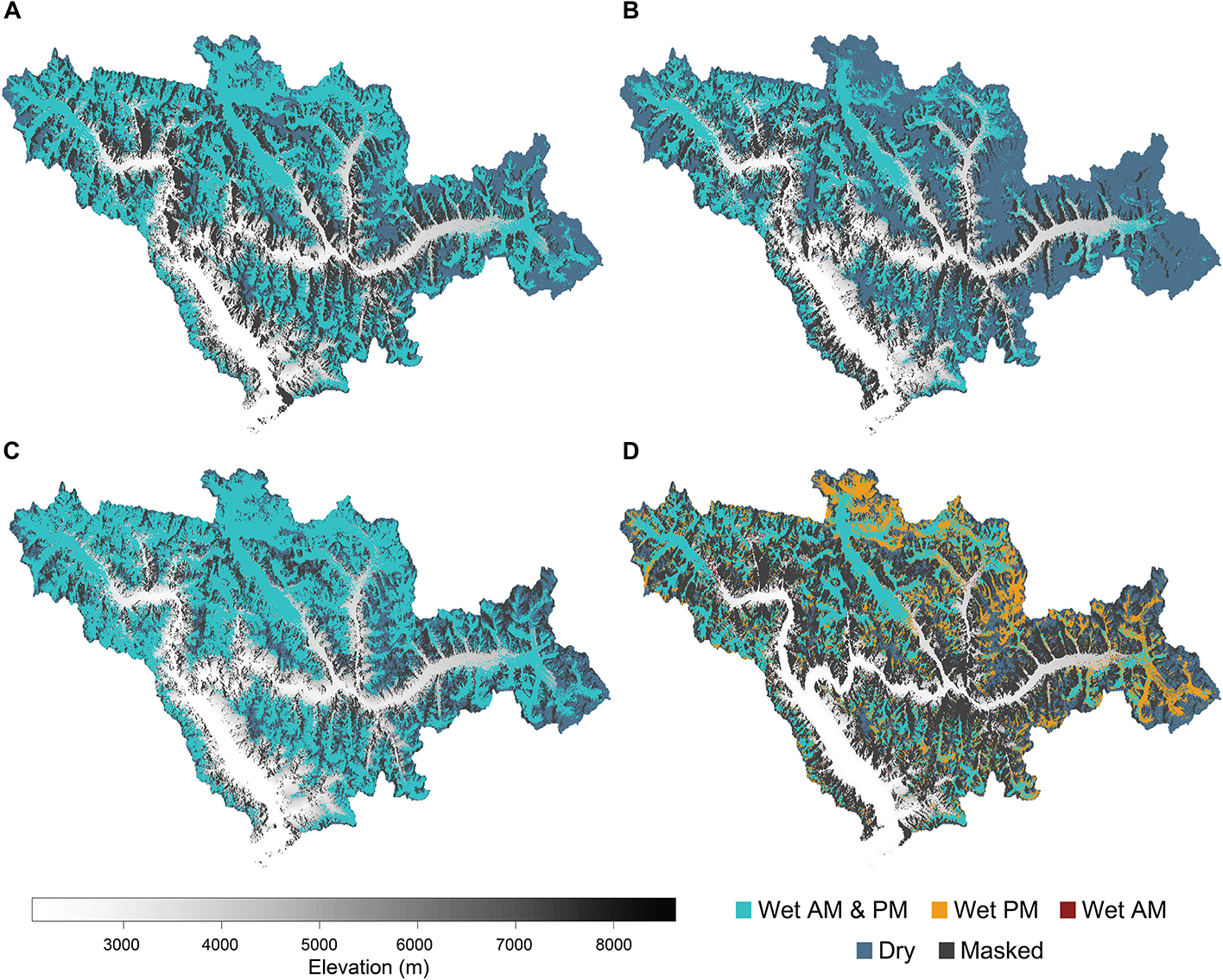
Figure 3. Image May 12–13, 2017. Resulting image from the pixel classification process for (A) Ascending pass. (B) Descending pass. (C) Combined orbits for wet snow. Panel (D) Shows the result of diurnally differing pixel classifications for this same image pair.
Secondly, we develop a “Diurnal Image” (Figure 3D) to examine pixels with differing designations in evening versus morning passes. A pixel-wise comparison between evening and morning images results in a classification into one of four main categories: (1) pixels that register as wet for both evening and morning acquisitions, (2) pixels that register as wet in the evening but not the morning after, (3) pixels that register as wet in the morning but not the evening before, and (4) pixels that do not register as wet. As in our Combined Image approach, pixels that do not register as wet in either image are subcategorized further: pixels below the median elevation of wet snow are assumed snow free, whereas pixels above the median elevation of wet snow are assigned as “dry snow.” We continue to mask pixels beneath 3000 m.a.s.l. The decision-tree process for pixel categorization can be viewed in Figure 4. S1 postprocessing, pixel classification, and subsequent analyses are accomplished using R (R Core Team, 2017).
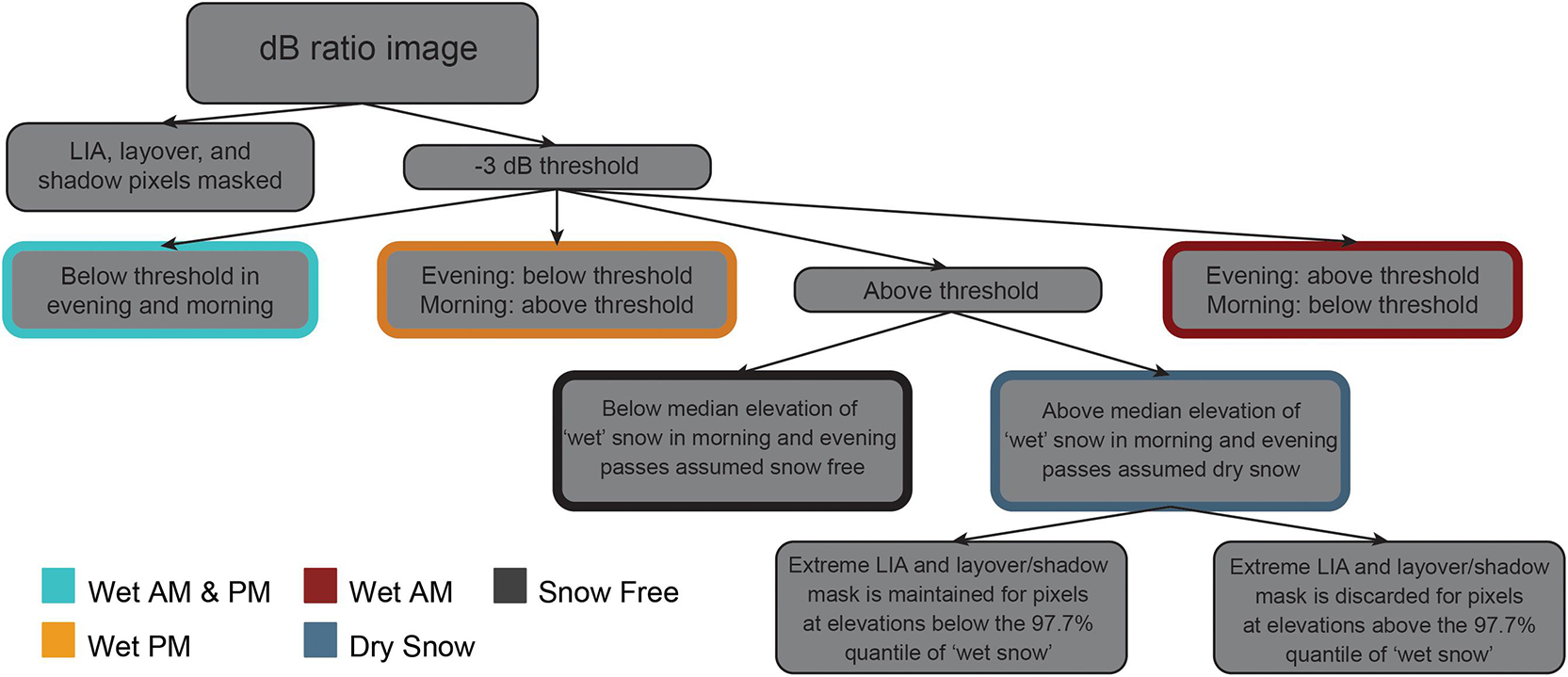
Figure 4. Pixel designation methodology for diurnal radar snow conditions.
S2 Snow Probability Map Comparison
As cloud cover is significant in the Shigar Watershed (Hasson et al., 2014), finding optical S2 imagery that is relatively cloud free and that also temporally coincides with S1 retrievals is a challenge for snow extent comparisons, even with frequent S2 overpass repeats. We select three dates in the 2017 and 2018 melt seasons with relatively cloud-free S2 images and near coincidental (within 1–2 days) S1 acquisitions: May 23, 2017, September 20, 2017, and June 12, 2018. For this comparison, S1 snow maps are generated from “Combined” images, which minimize masked areas due to layover and shadow or extreme local incidence angle. In this case, S1 pixel classifications are simplified to either snow covered (whether wet or dry), or snow free. Selected S2 Level-1C images were processed using the ESA third-party plug-in Sen2Cor, resulting in Level-2A images (Louis et al., 2016). Level-2A products are atmospherically corrected and come with quality bands that include snow and cloud confidence maps. For a pixel-wise comparison with S1 snow conditions maps, we assign any pixel with a snow confidence >50 (out of 100) as snow covered. We also mask any pixels with cloud confidence >70 (out of 100). Masked pixels in either S1 or S2 maps are consolidated, so only snow cover assignments are compared between the two products.
Wet Snow Qualitative Assessment
Temperature measurements at the Shigar DCP station from the ablation season of 2015 are qualitatively used to contextualize S1 snow wetness results. In order to estimate temperatures at different elevations in the Shigar Watershed, we apply a simple lapse rate of −6.8 degrees Celsius per 1000 m of elevation gain, a rate used by researchers in the nearby Hunza Basin (Immerzeel et al., 2012). Recognizing the limitation of a singular meteorological station, we include scaled temperatures solely to gauge whether our radar snow conditions are commensurate with reasonable estimated temperatures, and note that the derived temperatures should be interpreted qualitatively. For quantitative interpretation, a lapse rate better rooted in local environmental conditions must be determined. Minimum and maximum temperature measurements for 2015, scaled to the median elevation of the Shigar Watershed (4678 m.a.s.l), can be viewed in Figure 5.
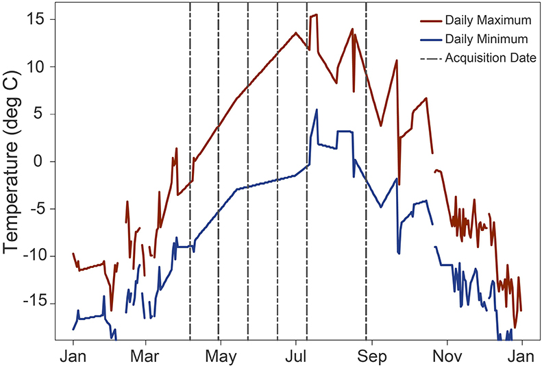
Figure 5. 2015 maximum and minimum temperature record from the Shigar DCP meteorological station (2367 m.a.s.l). Temperatures are scaled to the median elevation (4678 m.a.s.l) of the Shigar Watershed using a simple lapse rate of –6.8 degrees per 1000 m of elevation gain.
S1 wet snow extents are also compared to HMA ASCAT Freeze/Melt status products (Steiner and McDonald, 2018). The ASCAT Freeze/Melt product comes with 3 bands: freeze/thaw on land, freeze/melt on permanent snow and ice, and quality. We utilize the permanent snow/ice band, masking any pixels flagged for quality. As this daily product is available from January 1, 2009 through October 12, 2017, we compare it to S1 wet snow maps for ablation seasons 2015–2017.
Distribution Comparison of Diurnal Pixel Designation
Our diurnal pixel categorization perpetuates the simplicity of threshold-based wet snow designation, and merits examination. For example, a pixel with a ratio of −5 dB in the evening followed by −1 dB in the morning indicates a greater change in surface characteristics than a pixel with a diurnal comparison of −3.2 dB in the evening and −2.9 dB in the morning ratio value, yet these two cases will result in the same classification. Accordingly, we explore the distribution of ratio values for each of our pixel categories based on the classification process delineated in section “Pixel Classification.” For this analysis, we select the image from April 29–30, 2015, as it includes significant areas of each pixel categorization. For each pixel category, we compare the morning pass ratio values and also compare the absolute difference in ratio values from evening to morning. It is worth reiterating that by comparing ratios, we are devaluing specific backscatter values in order to focus on changes in surface characteristics from dry snow imagery taken from the same viewing geometry.
Results
Topographic Impacts
Extreme topography limits a significant portion of the Shigar Watershed from receiving a radar signal due to layover and shadow (Figure 6). Pixels masked due to extreme local incidence angle significantly increase the area without measurement. For ascending orbital passes, 1917 km2 or approximately 27% of the total watershed area is affected by radar layover or shadow. Along with masked pixels for extreme local incidence angles, the total area lost is 2374 km2, about 34% of the total watershed area. Descending orbital passes show a similar pattern, with 1872 km2 in layover or shadow and, including extreme local incidence angle, a total of 2400 km2 or 34% of watershed area masked. Combined Wet Snow images, created when ascending and descending passes are acquired within 12 h of each other, significantly reduce layover and shadow area to 705 km2, about 10% of watershed area. Including masked pixels for extreme local incidence angle, the area of lost information approximates 21% of the total area.
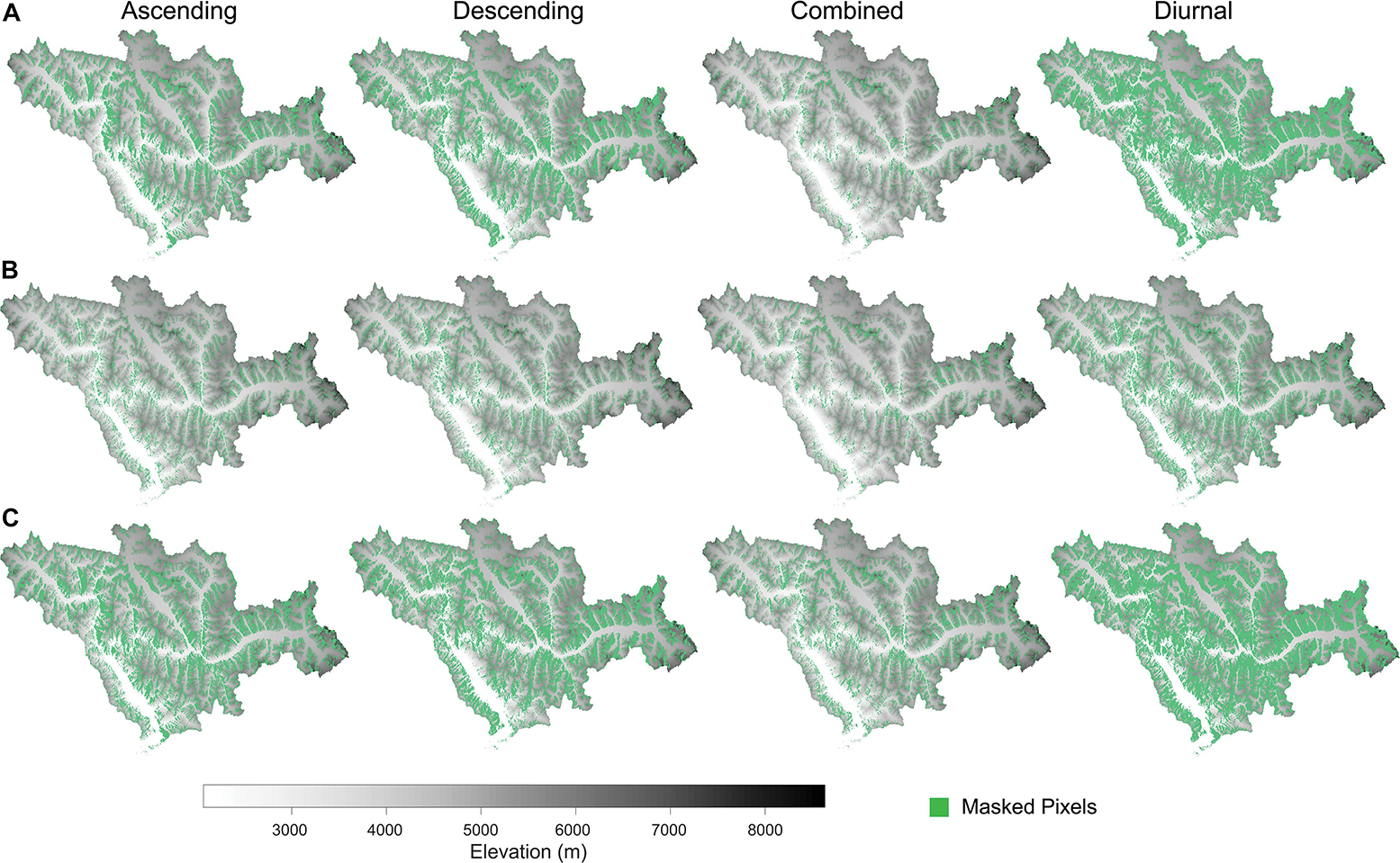
Figure 6. Areas lost due to (A) layover and shadow. (B) Extreme local incidence angle. (C) The two combined for separate orbital passes, combined pass images, and diurnal images.
To explore the diurnal contrast in backscatter from ascending and descending passes, lost information must be accumulated rather than reduced: to compare pixel values, information from both ascending and descending passes must be present, and extreme local incidence angles must also be eliminated from both orbital passes. Pixel-wise comparison to create Diurnal Images results in a total masked area of 3301 km2, approximately 47% of the Shigar Watershed. Near polar orbits of the S1 satellites result in blocked pixels that lie primarily in east and west aspects for the Diurnal Image. Figure 6 displays a map of masked pixels according to orbital pass and orbital compilation. Because of similar satellite viewing geometries, masked areas show very little inter-image change, with a maximum standard deviation of 10 km2 for total masked area for any melt season.
Radar Threshold Impact on Pixel Classification
Diurnal snow conditions maps with dB thresholds of −2 and −3 dB can be viewed in Supplementary Figure S1. The −2 dB ratio threshold, which reflects a smaller inter-image change than the −3 dB threshold, results in more pixels that are classified as “wet” snow (1260.7 km2 compared to 1047.6 km2 on the date analyzed in Supplementary Figure S1). For diurnally differing pixels, a −2 dB threshold increases the area of pixels classified as wet in the evening but not in the morning by 22.87 km2, or about 5.7%. For pixels that are not classified as wet in the evening but do register as wet in the morning, a −2 dB threshold increases the total area by 61.29 km2, an increase of about 36.1%.
Sentinel-2 Snow and Cloud Confidence Maps
Figure 7 offers a comparison of S1 and S2 snow cover maps for three dates in 2017 and 2018 (section “S2 Snow Probability Map Comparison”). Snow map comparisons yield a pixel-to pixel accuracy of 89.2%, 84.1%, and 86.8%, respectively. For both 2017 images, the pixel discrepancies are evenly distributed between sensors. For the 2018 image, the S1 snow map shows more pixels as snow covered (approximately 10% of compared pixels) than S2. Confusion matrices for each image comparison are visible in Supplementary Tables S2–S4.
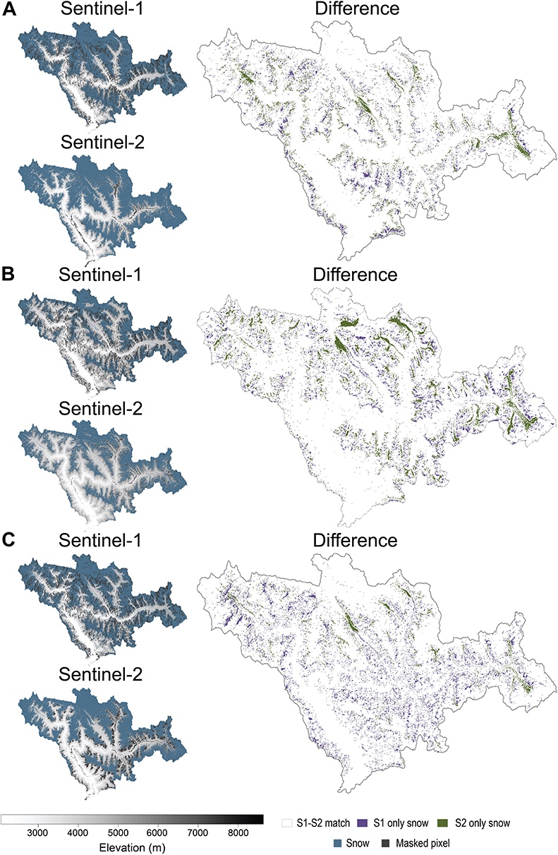
Figure 7. Sentinel-1 and Sentinel-2 snow extent comparisons for 3 dates. (A) S1: May 23–24, 2017, S2: May 23, 2017. (B) S1: September 21–22, 2017, S2: September 20, 2017. (C) S1: June 12–13, 2018, S2: June 12, 2018. Difference maps are also provided for each comparison.
HMA ASCAT Freeze/Melt Status Comparison
Time series of HMA ASCAT Freeze/Melt Status for melt seasons 2015–2017 can be viewed in Supplementary Figures S2–S4. The S1 and ASCAT results show good spatial agreement in wet snow identification. For each ablation season, melt signals first appear in both S1 and ASCAT products in the northwest region of the Shigar Watershed (Chogo Lungma Glacier). The high-altitude Baltoro Glacier in the east, which holds multiple 8,000 meter peaks such as K2 and Broad Peak, is the last to show surface snowmelt, although each ablation season does classify “wet” pixels in the higher elevations of the watershed for both products.
Combined Image Season Comparison
A seasonal comparison of wet snow evolution for ablation seasons of 2015, 2016, 2017, and 2018 is detailed in Figure 8. Individual wet snow maps for each season are in Supplementary Figures S5–S8. To avoid outlying pixels, we adopt the minimum and maximum elevations of wet snow to be at 2.3% and 97.7% quantiles, respectively (approximating two standard deviations above and below the mean elevation for normal distributions). The elevation distribution of the lower 5% quantile of wet snow can be viewed in Supplementary Figure S9. The minimum elevation of wet snow, or the transient snow line (TSL), is tracked through each season (Figure 8, left column). Aside from some variability in the early ablation season, the TSL shows a similar rate of rise for seasons 2015–2017, with elevations peaking at approximately 4200 m in mid-July or early August each year. The maximum rate of rise occurs early in the melt season each year, and approximates 20 m day–1. 2017 shows the most rapid rate of rise, approximately 35 m day–1 in early April. 2018 shows a much slower rate of rise than the other seasons (a maximum of approximately 13 m day–1), and also a lower maximum TSL of 3880 m in early August. For each season, TSL elevations begin to generally decrease in late July or early August.
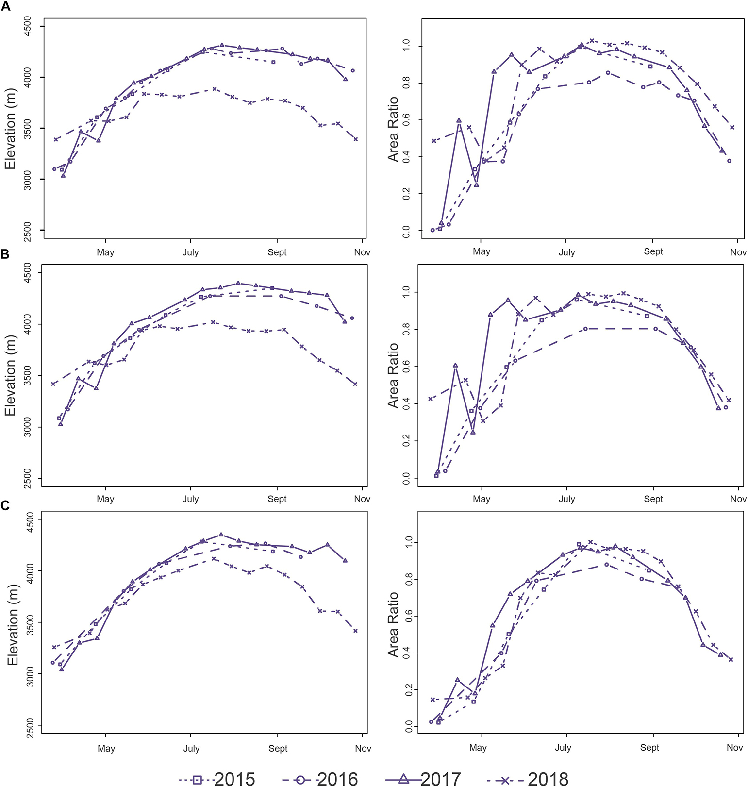
Figure 8. Combined image wet snow seasonal comparison of wet snow minimum elevation (2.3% quantile) in the left column and area ratio (area scaled to the total calculated snow cover area for that date) in the right column. (A) Combined ascending and descending passes. (B) Ascending orbital pass, at approximately 18:00 local time. (C) Descending orbital pass, at approximately 6:00 local time.
We also compare “area ratios” – or the area of wet snow normalized to the total classified snow cover area for that date – which show strong interannual variability, most evident in the rate of early season development (Figure 8, right column). Each year shows peak wet snow area ratio in July – August, with wet snow accounting for a ratio of nearly 0.90 of the total snow covered area. 2016 shows a lower maximum wet snow area ratio, approximately 0.77 in early August. In April and May, wet snow area ratio shows prominent inter-image fluctuations; in 2017, for example, area ratio drops from 0.54 to 0.23 from April 19–20 to April 30-May 1 images, thereafter increasing to 0.77 on May 12–13. Beginning in August of each year, wet snow area ratio decreases, although 2016 shows variability in late ablation season.
To explore the justification of comparing diurnal differences in radar-assessed snow conditions, we generate the same seasonal comparisons of transient snowline and area ratio, separated by orbital pass (Figures 8B,C). TSL elevations are generally corroborated by separate orbital passes, although the maximum TSL elevation for each season occurs in the ascending pass (approximately 18:00 local time) and generally occurs later in the season for the ascending pass. However, orbital pass variability is much more prominent in area ratio measurements. For both 2017 and 2018, the ascending pass wet snow area ratio shows strong variability through the month of June in contrast to the descending pass.
Diurnal Image Comparison
Distribution Comparison of Pixel Designation
We first focus on the morning ratio distribution for each pixel designation, as their value will ultimately determine pixel categorization. Table 1 details the median value of each pixel classification morning ratio, as well as its median absolute deviation. Pixels classified as wet both evening and morning measure a median morning ratio of −5.0 with a median absolute deviation of 2.0 dB. In contrast, pixels that register as wet in the evening but not in the morning measure a median morning ratio of −0.48, with a median absolute deviation of 1.7 dB. Finally, pixels that are not designated as wet in the evening, but wet in the morning pass show a median morning ratio of −3.6, with a median absolute deviation of 0.9 dB.
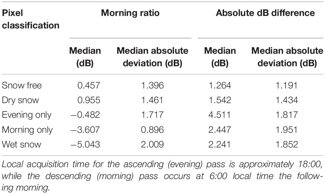
Table 1. Pixel classification distribution values.
We also explore the absolute difference of overnight change in ratio values, as these provide an indication of changes in surface conditions (Table 1). Pixels that register as wet in both evening and morning passes show a median absolute difference of 2.2, and a median absolute deviation of 1.9 dB. Pixels that register as wet in the evening but not the following morning measure an overnight median absolute difference of 4.5, and a median absolute deviation of 1.8 dB. Finally, pixels that are not classified as wet in the evening but as wet in the morning have a median absolute difference of 2.4, and a median absolute deviation of 2.0 dB.
Pixels that register as wet both evening and morning typically have morning ratio values well below the −3 dB threshold, and show relatively small overnight change in ratio values. For the remainder of this study, we refer to these pixels as “wet snow.” Pixels that register as wet in the evening but not in the morning measure a morning ratio value that is well above the −3 dB threshold, and show a much greater overnight change than any other pixel classification; we will subsequently refer to these pixels as “diurnally different.” Pixels that do not register as wet in the evening but do in the morning show a morning ratio value close to the – 3dB threshold, and also show less change overnight than diurnally different pixels. They also have a small presence in this classification scheme: for example, in 2017 the average area for this pixel classification is 96 km2 (1.4% of watershed area). For these reasons, we will not analyze them further in this study; future field study could clarify the conditions responsible for this phenomenon. However, we do include these pixels in diurnal difference images (Figures 9–11) so their spatiotemporal context is clear throughout the melt season.
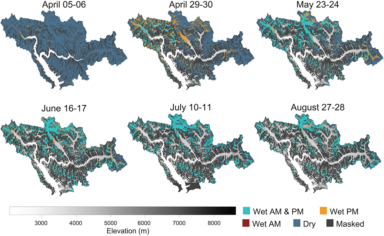
Figure 9. 2015 melt season radar snow conditions.
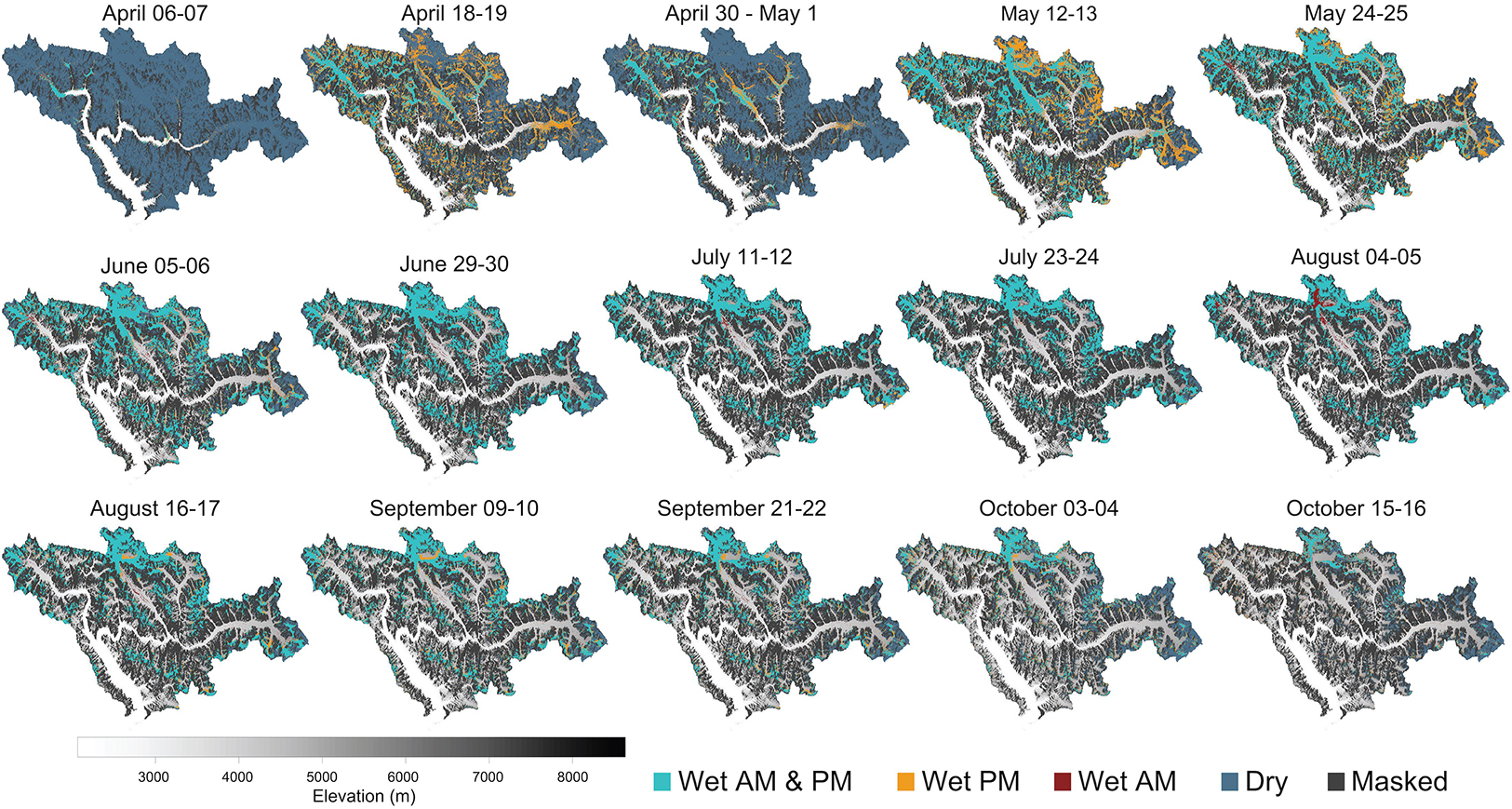
Figure 10. 2017 melt season radar snow conditions.
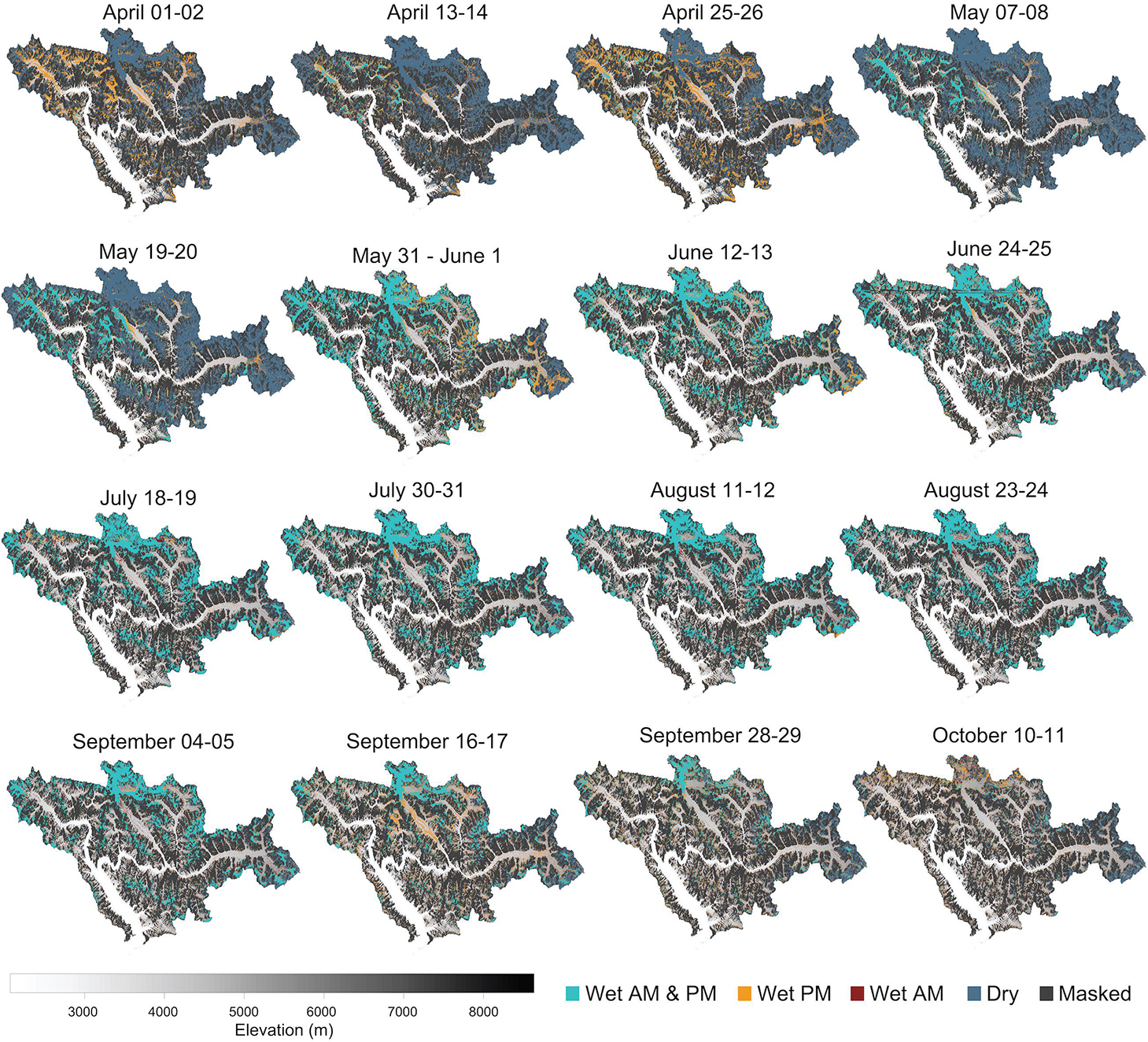
Figure 11. 2018 melt season radar snow conditions.
2015, 2017, and 2018 Diurnal Seasonal Snow Conditions
We compile six diurnal difference images from the ablation season of 2015 (Figure 9), and due to an accomplished ramp up and exploitation phase for S1-A and -B, 15 images for 2017 (Figure 10) and 16 images for 2018 melt seasons (Figure 11). 2016 acquisition patterns do not enable diurnal comparison, although melt images are available for this season in Supplementary Figure S6.
As we are interested in the areal and altitudinal distribution of diurnally different radar snow conditions, we explore the seasonal evolution of their median rather than minimum elevation as we did with the Combined Pass. A seasonal comparison of the median elevation and area ratio for each pixel designation can be viewed in Figure 12. For each season, the median elevation of diurnally differing pixels remains above that of wet pixels until about mid June, after which the median elevation of wet pixels remains slightly higher. The greatest variability in median elevations for each pixel classification occurs in early and late ablation season. The maximum median elevation for diurnally differing pixels is 5187 m.as.l. on May 24–25, 2017.
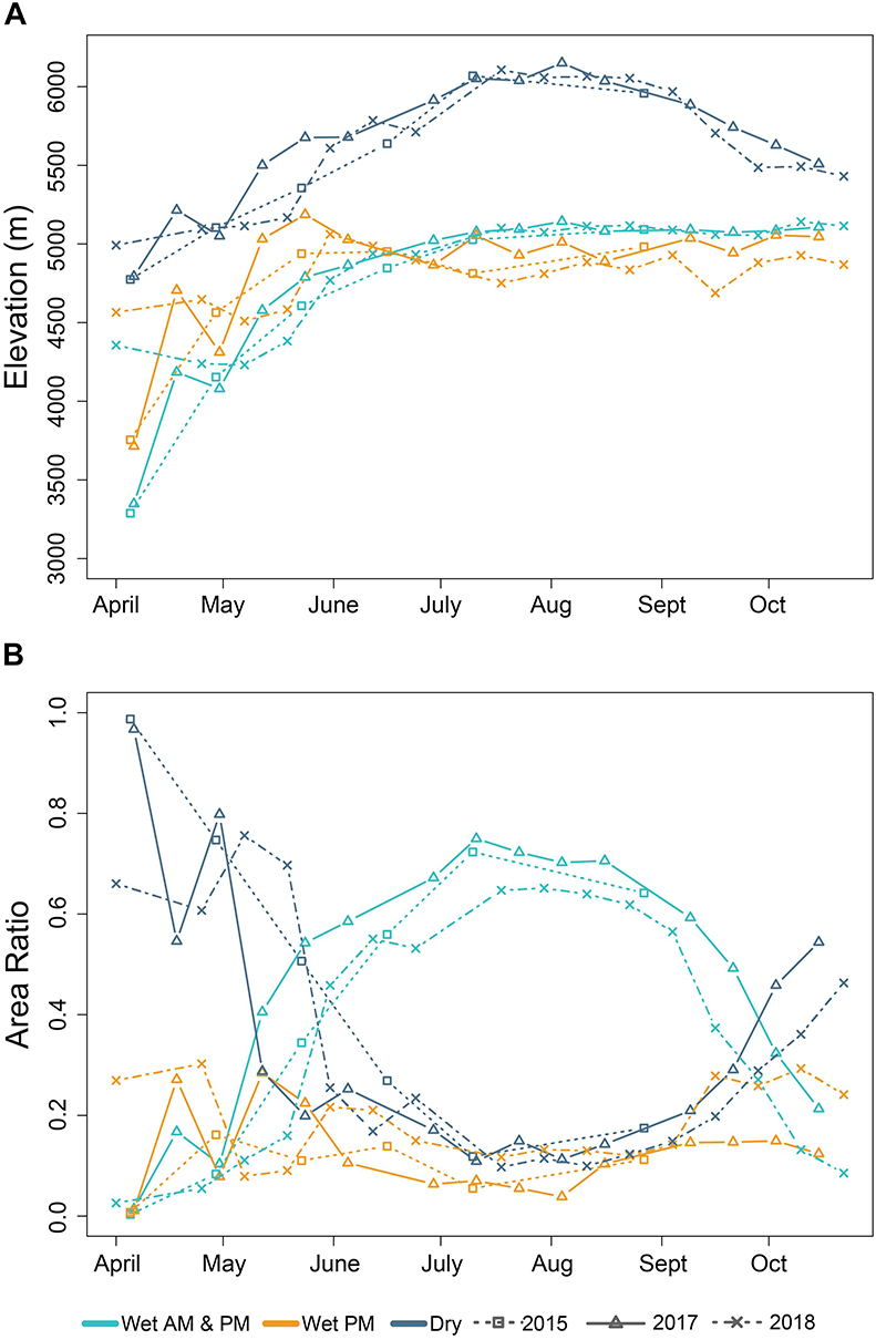
Figure 12. Melt season diurnal radar snow conditions comparison for ablation seasons 2015, 2017, and 2018. (A) Median elevation, and (B) area ratio (area scaled to the total calculated snow cover area for that date).
A comparison of snow condition area ratios (Figure 12) also shows most variability occurring in early ablation season. 2017 and 2018 diurnally different pixel area ratios are as high as 0.27 and 0.30, respectively, in late April. As melt season progresses for each year, wet snow dominates total snow covered area, showing significant decreases starting in September.
Discussion
Radar Threshold Impact on Pixel Classification
While decreasing the threshold value for the change in backscatter to −2 dB has an impact on wet snow total area, the overall spatiotemporal pattern of pixel classification is not significantly altered when the threshold is varied (Supplementary Figure S1). It is noteworthy that the area of pixels that are classified as diurnaly different are the least impacted by a change in threshold value. Pixels classified not wet in the evening but wet in the morning are the most impacted by a change in threshold, confirming that they are closer to the threshold value and therefore a noisier signal. A lack of in situ snow wetness validations supports a more conservative −3 dB threshold until field measurements prescribe an appropriate local threshold.
Optical Image Snow Extent Comparison
S1 snow extent agrees quite well with S2 snow confidence maps, with some consistent discrepancies (Figure 7). S2 regularly classifies snow cover on glacier tongues that S1 maps do not corroborate; this is most prominent in the late ablation season comparison on September 20–22, 2017 (Figure 7B). On the other hand, discrepancies in which only S1 pixels are classified as snow covered often occur off of glacier tongues on steeper hillsides in this rugged catchment. Because ‘dry snow’ S1 pixel classification is determined in relation to the elevation of pixels determined to be “wet,” steep rocky slopes and other land covers are not taken into account – a limitation of this methodology. Additionally, this S1 snow extent methodology is likely inadequate in early or late melt season, when the spatial extent of dry snow is far greater than that of wet snow (a similar issue described in Storvold and Malnes, 2004). A more accurate snow cover map could likely be achieved by incorporating cloud-free optical imagery or multiple SAR polarizations. However, when wet snow is present, SAR sensor identification of snow cover regardless of cloud cover is valuable, especially considering the common misclassification of cloud, ice, and snow pixels in optical imagery. In these image comparisons, S1 masked pixels calculate greater area than S2 masked pixels (derived from S2 cloud confidence values). However, S2 masked cloud pixels are often located low on glacier tongues or along the Shigar River, in spatial patterns suggesting potential pixel misclassification, further illustrating the challenge of spectrally separating clouds, ice, water, and snow.
Wet Snow Conditions
S1 snow conditions show an appreciable extent of wet snow during each ablation season, notable for one of the highest altitude watersheds in HMA. While a single meteorological station does not suffice for quantitative analyses of temperatures, it does offer qualitative validation for whether S1 snow classifications are reasonable. The daily maximum and minimum temperatures for 2015, scaled to the median elevation of the Shigar Watershed (4768 m.a.s.l), show reasonable maximum temperature values for daytime snowmelt to occur throughout the watershed. The estimated minimum temperatures at the median altitude are also reasonable when considering diurnal differences in snow conditions, as they remain below 0 degrees C until nearly July.
HMA ASCAT Freeze/Melt products also corroborate the spatial extent of S1 wet snow for each season (Supplementary Figures S2–S4). Pixel-to-pixel comparison ASCAT and S1 products is not ideal as most of the Shigar Watershed has been assigned pixel classifications as “permanent snow or ice” in the ASCAT product. With that designation, a given pixel is either given a “melt” or “freeze” status; in other words, as melt out reveals bare glacier ice, reducing the extent of S1 snow conditions maps, ASCAT will still assign each pixel as either frozen or melting. Each season, however, shows both products determining melt occurring at high elevations in the Shigar Watershed. The maximum elevation for S1 wet snow typically reaches nearly 6000 m.a.s.l, although in 2017 the maximum wet snow reached 6245 m.a.s.l in July. Abnormally warm temperatures for that season were confirmed by climbers on the Choktoi Glacier, who had to retreat from their objectives because above-freezing overnight temperatures resulted in unsafe climbing conditions (personal communication, 2017).
Diurnal Radar Comparisons
Beyond the quantitative indications of changing surface conditions discussed in section “Distribution Comparison of Pixel Designation,” on a watershed scale, the spatial and temporal context of pixel designation matches what we would expect to see from a snowpack exposed to surface energy balance changes throughout the melt season. In 2015 (Figure 9), the early April image is dominated by dry snow. By the end of the month, both wet and diurnally different pixels are present throughout the watershed. From May, wet snow increases in area throughout the watershed until late August, when melt out appears to have occurred except for at the highest altitudes.
The 2017 melt season shows a similar evolution (Figure 10), although early season comparison suggests more rapidly developed melt conditions and greater volatility than 2015. After strong early season melt signals, with large areas of both wet as well as diurnally different signals, images through June and July are increasingly dominated by wet pixels. Classification patterns from August onward show a strong signal of snow melt out, exposing glacier ice to surface conditions.
2018 shows prominent areas of diurnally different pixels in early and late April (Figure 11). Compared to the 2017 season, however, snowmelt develops more slowly in the month of May, also evident in area ratio comparisons in Figure 12B. Similar to previous seasons, wet snow begins to dominate the total snow cover area beginning in late June. This corresponds with the time that median elevation of diurnally different pixels drops beneath that of wet pixels, intimating a seasonal shift.
The seasonal spatial development of pixel classifications, along with distinct distribution values discussed in section “Distribution Comparison of Pixel Designation,” both support our hypothesis that diurnally differing radar signals indicate changes in surface conditions. Considering radar sensitivity to surface roughness and dielectric properties, physical surface changes could potentially be associated with: (1) a change in surface roughness, (2) a change in liquid water content due to overnight drainage, or (3) a change in liquid water content due to refreeze. Refreezing could either involve the entirety of snowpack liquid water content (i.e., refreezing of wet layers over a dry snowpack), or a thin surface layer of refreeze overlying wet snow (Mätzler and Hüppi, 1989).
Although surface roughness of wet snow can impact backscatter values late in the melt season (Nagler, 1996), the early season prevalence of diurnally different pixels limits the feasibility of explanation (1). Significant changes in surface roughness overnight also seem unlikely to occur. Explanations (2) and (3), both involving changes in liquid water content of the snowpack, are worth consideration.
In early melt seasons of 2015, 2017, and 2018, diurnally different pixels occur at higher elevations than wet snow. As saturated snow does not store water beyond its capillary pressure requirements over time (e.g., DeWalle and Rango, 2008; Samimi and Marshall, 2017), a change in liquid water content due to overnight drainage does not necessarily explain the spatial context of early season diurnal changes in radar response. In other words, if the entire snowpack typically drains to its irreducible water content overnight, explanation (2) does not explain diurnally differing pixels occurring at higher elevations than wet snow in the early melt season. However, a change in liquid water content due to refreeze does offer a reasonable explanation for early season pixel designations. Recall that Mätzler and Hüppi (1989) found C-band backscatter to be sensitive to refrozen crusts over a dry snowpack, but relatively insensitive to refrozen crusts over a ripe snowpack (1989). As melt-freeze crusts over a ripe snowpack can occur throughout the melt season (Macelloni et al., 2005; Samimi and Marshall, 2017), the early season prevalence of diurnally different radar signals seems most likely due to a refreeze of liquid water overlying a dry snowpack. If this is the case, diurnally differing radar signals can offer important insight into portions of the snowpack that are experiencing surface melt but not yet contributing to runoff, or still in the warming and ripening phases. Beyond the spatiotemporal context of diurnally different pixels in the Shigar Watershed, this hypothesis is corroborated with recent findings in the Alps using S1 backscatter to identify snow melt periods of moistening, during which the authors point out a diurnal difference in backscatter indicating afternoon melt and overnight refreeze before the snowpack has become isothermal (Marin et al. in discusson).
The spatial context of diurnally different radar signals in late ablation season merits a separate evaluation of potential surface condition changes. Again, overnight changes in surface roughness make (1) an unlikely explanation. A reduction in liquid water content due to overnight drainage or surface refreeze does allow greater radar penetration depth, and in the case of a very thin snowpack could result in radar interaction with the snow-ground or snow-ice interface during the morning pass, thereby increasing backscatter values (e.g., Nagler, 1996). This hypothesis is also reasonable considering the spatiotemporal context of pixels that register as wet in the morning but not the evening before, for example on August 4–5, 2017 (Figure 10): in this image, morning wet pixels cluster around Lukpe Lawo, a basin high on the Biafo Glacier commonly known as “Snow Lake.” Overnight drainage from a very wet snowpack at higher elevations could result in melt ponds growing overnight.
Summary and Next Steps
We have explored the topographic effects of layover, shadow, and extreme local incidence angle on SAR imagery in the Shigar Watershed of the Karakoram Mountains. Combined Images mask 21% of pixels, while Diurnal Images mask 47% of the total watershed area. Layover and shadow impact primarily east and west aspects, although topographic impacts do not prevent observation of seasonal trends in snow conditions even in this challenging terrain.
Comparing our SAR-derived snow maps with S2-derived snow maps shows good pixel-wise agreement of 84–89% at different times in the melt season. This agreement encourages the use of SAR-derived snow conditions maps in areas with significant cloud cover, for example in monsoonal regions of HMA. We have developed SAR wet snow maps in order to track interannual variation in transient snow line altitudes and wet snow area ratios for the ablation seasons of 2015–2018. Transient snow lines show similar trends, while wet snow area ratios show strong interannual variability, particularly in early melt season.
Additionally, we have explored diurnal differences in radar signals for coincident orbital passes in the melt seasons of 2015, 2017, and 2018. Early ablation season variability is evident comparing each ablation season, with 2017 showing much stronger and more rapid development of wet and diurnally different pixels. Examination of pixel classification distributions suggests that diurnally different pixels are indicative of overnight changes in snow surface conditions. Additional validation is necessary, but the seasonal evolution and spatial context of diurnally differing radar signals in the early ablation season may be due to overnight melt-freeze crusts overlying a dry snowpack, a valuable indication of a supraglacial snowpack in warming or ripening phases and not yet contributing to runoff. If this is the case, diurnally differing SAR signals could offer constraining information for physically based energy balance and runoff models in an area with sparse measurement. Field measurements of snow wetness profiles during melt-refreeze cycles coinciding with satellite overpasses will be pursued as a next step, as well as incorporating these data into energy balance and runoff models.
Data Availability Statement
Publicly available datasets were analyzed in this study. SAR data can be found here: https://vertex.daac.asf.alaska.edu/.
Author Contributions
JL, RF, and SR were involved throughout the research, analysis, and manuscript process. HM and ED provided insight and feedback early in the analysis process, and provided ongoing manuscript feedback. EB was involved in establishing the research and analysis processes. MH provided the meteorological data for the study area, as well as feedback through the manuscript process.
Funding
JL and RF are grateful for funding for this research by NASA award number NNX16AK54G. JL would like to acknowledge the Pakistan’s Global Change Impact Studies Centre for providing the meteorological data and funding her participation in the Science-Policy Conference on Climate Change in December 2017, at which preliminary findings of this research were presented.
Conflict of Interest
The authors declare that the research was conducted in the absence of any commercial or financial relationships that could be construed as a potential conflict of interest.
Acknowledgments
The authors would like to thank the reviewers who provided valuable feedback through the review process.
Supplementary Material
The Supplementary Material for this article can be found online at: https://www.frontiersin.org/articles/10.3389/feart.2019.00318/full#supplementary-material
References
Archer, D. R., and Fowler, H. J. (2004). Spatial and temporal variations in precipitation in the Upper Indus Basin, global teleconnections and hydrological implications. Hydrol. Earth Syst. Sci. Discuss. 8, 47–61. doi: 10.5194/hess-8-47-2004
Bales, R. C., Molotch, N. P., Painter, T. H., Dettinger, M. D., Robert, R., and Dozier, J. (2006). Mountain hydrology of the western United States. Water Resour. Res. 42, doi: 10.1073/pnas.1802316115
Barnett, T. P., Adam, J. C., and Lettenmaier, D. P. (2005). Potential impacts of a warming climate on water availability in snow-dominated regions. Nature 438:303. doi: 10.1038/nature04141
Bocchiola, D., Diolaiuti, G. A., Soncini, A., Mihalcea, C., D’agata, C., Mayer, C., et al. (2011). Prediction of future hydrological regimes in poorly gauged high altitude basins: the case study of the upper Indus, Pakistan. Hydrol. Earth Syst. Sci. 15, 2059–2075. doi: 10.5194/hess-15-2059-2011
Brun, E. (1989). Investigation on wet-snow metamorphism in respect of liquid-water content. Ann. Glaciol. 13, 22–26. doi: 10.1017/s0260305500007576
Brun, F., Berthier, E., Wagnon, P., Kääb, A., and Treichler, D. (2017). A spatially resolved estimate of High Mountain Asia glacier mass balances from 2000 to 2016. Nat. Geosci. 10:668. doi: 10.1038/NGEO2999
Chen, Y., Xu, C., Chen, Y., Li, W., and Liu, J. (2010). Response of glacial-lake outburst floods to climate change in the Yarkant River basin on northern slope of Karakoram Mountains. China. Q. Int. 226, 75–81. doi: 10.1016/j.quaint.2010.01.003
Cogley, J. G. (2011). Present and future states of Himalaya and Karakoram glaciers. Ann. Glaciol. 52, 69–73. doi: 10.3189/172756411799096277
Colbeck, S. C. (1976). An analysis of water flow in dry snow. Water Resour. Res. 12, 523–527. doi: 10.1029/wr012i003p00523
Core Writing Team, Pachauri, R. K., and Meyer, L. A. (2014). “IPCC, 2014: climate change 2014: synthesis report,” in Contribution of Working Groups I. II and III to the Fifth Assessment Report of the intergovernmental panel on Climate Change. Geneva: IPCC, 151.
Cuffey, K. M., and Paterson, W. S. B. (2010). The Physics of Glaciers. Cambridge, MA: Academic Press.
Déry, S. J., and Brown, R. D. (2007). Recent Northern Hemisphere snow cover extent trends and implications for the snow-albedo feedback. Geophys. Res. Lett. 34
DeWalle, D. R., and Rango, A. (2008). Principles of Snow Hydrology. Cambridge: Cambridge University Press.
Early, D. S., and Long, D. G. (2001). Image reconstruction and enhanced resolution imaging from irregular samples. IEEE Trans. Geosci. Remote Sens. 39, 291–302. doi: 10.1371/journal.pone.0035299
Fahnestock, M., Bindschadler, R., Kwok, R., and Jezek, K. (1993). Greenland ice sheet surface properties and ice dynamics from ERS-1 SAR imagery. Science 262, 1530–1534. doi: 10.1126/science.262.5139.1530
Floricioiu, D., and Rott, H. (2001). Seasonal and short-term variability of multifrequency, polarimetric radar backscatter of alpine terrain from SIR-C/X-SAR and AIRSAR data. IEEE Trans. Geosci. Remote Sens. 39, 2634–2648. doi: 10.1109/36.974998
Forsythe, N., Fowler, H. J., Li, X. F., Blenkinsop, S., and Pritchard, D. (2017). Karakoram temperature and glacial melt driven by regional atmospheric circulation variability. Nat. Clim. Change 7:664. doi: 10.1038/nclimate3361
Fowler, H. J., and Archer, D. R. (2006). Conflicting signals of climatic change in the Upper Indus Basin. J. Clim. 19, 4276–4293. doi: 10.1175/jcli3860.1
Gardelle, J., Berthier, E., and Arnaud, Y. (2012a). Impact of resolution and radar penetration on glacier elevation changes computed from DEM differencing. J. Glaciol. 58, 419–422. doi: 10.3189/2012jog11j175
Gardelle, J., Berthier, E., and Arnaud, Y. (2012b). Slight mass gain of Karakoram glaciers in the early twenty-first century. Nat. Geosci. 5, 322–325. doi: 10.1038/ngeo1450
Hall, D. K., and Riggs, G. A. (2010). “Normalized-difference snow index (NDSI),” in Encyclopedia of Snow, Ice and Glaciers. Encyclopedia of Earth Sciences Series, eds V. P. Singh, P. Singh, and U. K. Haritashya, (Dordrecht: Springer).
Hasson, S., Lucarini, V., Khan, M. R., Petitta, M., Bolch, T., and Gioli, G. (2014). Early 21st century snow cover state over the western river basins of he Indus River system. Hydrol. Earth Syst. Sci. 18, 4077–4100. doi: 10.5194/hess-18-4077-2014
Heilig, A., Mitterer, C., Schmid, L., Wever, N., Schweizer, J., Marshall, H.-P., et al. (2015). Seasonal and diurnal cycles of liquid water in snow—Measurements and modeling. J. Geophys. Res. 120, 2139–2154. doi: 10.1002/2015jf003593
Hewitt, K. (2005). The Karakoram anomaly? Glacier expansion and the ‘elevation effect,’Karakoram Himalaya. Mountain Res. Dev. 25, 332–340. doi: 10.1002/2017GL076158
Hewitt, K. (2011). Glacier change, concentration, and elevation effects in the Karakoram Himalaya, Upper Indus Basin. Mountain Res. Dev. 31, 188–200. doi: 10.1659/mrd-journal-d-11-00020.1
Hewitt, K., Wake, C. P., Young, G. J., and David, C. (1989). Hydrological investigations at Biafo Glacier, Karakoram Range, Himalaya; an important source of water for the Indus River. Ann. Glaciol. 13, 103–108. doi: 10.1017/s0260305500007710
Immerzeel, W. W., Droogers, P., De Jong, S. M., and Bierkens, M. F. P. (2009). Large-scale monitoring of snow cover and runoff simulation in Himalayan river basins using remote sensing. Remote Sens. Environ. 113, 40–49. doi: 10.1016/j.rse.2008.08.010
Immerzeel, W. W., Pellicciotti, F., and Shrestha, A. B. (2012). Glaciers as a proxy to quantify the spatial distribution of precipitation in the Hunza basin. Mountain Res. Dev. 32, 30–38. doi: 10.1659/mrd-journal-d-11-00097.1
Immerzeel, W. W., Van Beek, L.P., and Bierkens, M. F. (2010). Climate change will affect the Asian water towers. Science 328, 1382–1385. doi: 10.1126/science.1183188
Immerzeel, W. W., Wanders, N., Lutz, A. F., Shea, J. M., and Bierkens, M. F. P. (2015). Reconciling high-altitude precipitation in the upper Indus basin with glacier mass balances and runoff. Hydrol. Earth Syst. Sci. 19, 4673–4687. doi: 10.5194/hess-19-4673-2015
Kääb, A., Treichler, D., Nuth, C., and Berthier, E. (2015). Brief Communication: contending estimates of 2003–2008 glacier mass balance over the Pamir–Karakoram–Himalaya. Cryosphere 9, 557–564. doi: 10.5194/tc-9-557-2015
Kapnick, S. B., Delworth, T. L., Ashfaq, M., Malyshev, S., and Milly, P. C. D. (2014). Snowfall less sensitive to warming in Karakoram than in Himalayas due to a unique seasonal cycle. Nat. Geosci. 7:834. doi: 10.1038/ngeo2269
Kattelmann, R., and Dozier, J. (1999). Observations of snowpack ripening in the Sierra Nevada. California, USA. J. Glaciol. 45, 409–416. doi: 10.1017/s002214300000126x
Langley, K., Hamran, S.-E., Høgda, K. A., Storvold, R., Brandt, O., Hagen, J. O., et al. (2007). Use of C-band ground penetrating radar to determine backscatter sources within glaciers. IEEE Trans. Geosci. Remote Sens. 45, 1236–1246. doi: 10.1109/tgrs.2007.892600
Lee, J.-S. (1981). Speckle analysis and smoothing of synthetic aperture radar images. Comput. Graph. Image Process. 17, 24–32. doi: 10.1016/s0146-664x(81)80005-6
Lin, H., Li, G., Cuo, L., Hooper, A., and Ye, Q. (2017). A decreasing glacier mass balance gradient from the edge of the Upper Tarim Basin to the Karakoram during 2000–2014. Sci. Rep. 7:6712.
Louis, J., Debaecker, V., Pflug, B., Main-Knorn, M., Bieniarz, J., Mueller-Wilm, U., et al. (2016). “Sentinel-2 sen2cor: L2a processor for users,” in Proceedings of the Living Planet Symposium, (Prague: Czech Republic), 9–13.
Macelloni, G., Paloscia, S., Pampaloni, P., Brogioni, M., Ranzi, R., and Crepaz, A. (2005). Monitoring of melting refreezing cycles of snow with microwave radiometers: the Microwave Alpine Snow Melting Experiment (MASMEx 2002-2003). IEEE Trans. Geosci. Remote Sens. 43, 2431–2442. doi: 10.1109/tgrs.2005.855070
Martinec, J., and Rango, A. (1991). Indirect evaluation of snow reserves in mountain basins. IAHS Publ. 205, 111–119.
Mätzler, C. (1987). Applications of the interaction of microwaves with the natural snow cover. Remote Sens. Rev. 2, 259–387. doi: 10.1080/02757258709532086
Mätzler, C., and Hüppi, R. (1989). Review of signature studies for microwave remote sensing of snowpacks. Adv. Space Res. 9, 253–265. doi: 10.1016/0273-1177(89)90493-6
Maussion, F., Scherer, D., Mölg, T., Collier, E., Curio, J., and Finkelnburg, R. (2014). Precipitation seasonality and variability over the Tibetan Plateau as resolved by the High Asia Reanalysis. J. Clim. 27, 1910–1927. doi: 10.1175/JCLI-D-13-00282.1
Meier, M., and Post, A. (1995). Glaciers: A Water Resource (Rep.). Washington, D.C: U.S. Government Printing Office.
Mukhopadhyay, B., and Khan, A. (2014). Rising river flows and glacial mass balance in central Karakoram. J. Hydrol. 513, 192–203. doi: 10.1016/j.jhydrol.2014.03.042
Mukhopadhyay, B., and Khan, A. (2015). A reevaluation of the snowmelt and glacial melt in river flows within Upper Indus Basin and its significance in a changing climate. J. Hydrol. 527, 119–132. doi: 10.1016/j.jhydrol.2015.04.045
Nagler, T. (1996). Methods and Analysis of Synthetic Aperture Radar Data from ERS-1 and X-SAR for Snow and Glacier Applications. Innsbruck: Diss. Leopold-Franzens-Universität Innsbruck.
Nagler, T., and Rott, H. (1998). “SAR tools for snowmelt modelling in the project HydAlp,” in Proceedings of thr Geoscience and Remote Sensing Symposium Proceedings, 1998. IGARSS ’98. 1998 IEEE International, (Seattle, WA: IEEE).
Nagler, T., and Rott, H. (2000). Retrieval of wet snow by means of multitemporal SAR data. IEEE Trans. Geosci. Remote Sens. 38, 754–765. doi: 10.1109/36.842004
Nagler, T., Rott, H., Ripper, E., Bippus, G., and Hetzenecker, M. (2016). Advancements for snowmelt monitoring by means of sentinel-1 SAR. Remote Sens. 8:348. doi: 10.3390/rs8040348
Oerlemans, J. (2000). Analysis of a 3 year meteorological record from the ablation zone of Morteratschgletscher, Switzerland: energy and mass balance. J. Glaciol. 46, 571–579. doi: 10.3189/172756500781832657
Painter, T. H., Barrett, A. P., Landry, C. C., Neff, J. C., Cassidy, M. P., Lawrence, C. R., et al. (2007). Impact of disturbed desert soils on duration of mountain snow cover. Geophys. Res. Lett. 34:L12502.
Painter, T. H., McKenzie Skiles, S., Deems, J. S., Bryant, A. C., and Landry, C. C. (2012). Dust radiative forcing in snow of the Upper Colorado River Basin: 1. A 6 year record of energy balance, radiation, and dust concentrations. Water Res. Res. 48:7521. doi: 10.1073/pnas.0913139107
Parajka, J., and Blöschl, G. (2008). Spatio-temporal combination of MODIS images–potential for snow cover mapping. Water Resour. Res. 44:W03406.
Pfeffer, W. T., Arendt, A. A., Bliss, A., Bolch, T., Cogley, J. G., Gardner, A. X., et al. (2014). The Randolph Glacier Inventory: a globally complete inventory of glaciers. J. Glaciol. 60, 537–552. doi: 10.3189/2014jog13j176
Pfeffer, W. T., Illangasekare, T. H., and Meier, M. F. (1990). Analysis and modeling of melt-water refreezing in dry snow. J. Glaciol. 36, 238–246. doi: 10.1017/s0022143000009497
R Core Team, (2017). R: A Language and Environment for Statistical Computing. Vienna: R Foundation for Statistical Computing.
Ragettli, S., Pellicciotti, F., Bordoy, R., and Immerzeel, W. W. (2013). Sources of uncertainty in modeling the glaciohydrological response of a Karakoram watershed to climate change. Water Resour. Res. 49, 6048–6066. doi: 10.1002/wrcr.20450
Reber, B., Mätzler, C., and Schanda, E. (1987). Microwave signatures of snow crusts modelling and measurements. Int. J. Remote Sens. 8, 1649–1665. doi: 10.1080/01431168708954805
Reggiani, P., Coccia, G., and Mukhopadhyay, B. (2016). Predictive uncertainty estimation on a precipitation and temperature reanalysis ensemble for Shigar Basin. Central Karakoram. Water 8:263. doi: 10.3390/w8060263
RGI Consortium. (2017). “Randolph glacier inventory–a dataset of global glacier outlines: version 6.0,” in Technical Report, Global Land Ice Measurements from Space, (Colorado: Digital Media).
Richter, R., Louis, J., and Müller-Wilm, U. (2012). Sentinel-2 msi–level 2a products algorithm theoretical basis document. Eur. Space Agency 49, 1–72.
Rignot, E., Echelmeyer, K., and Krabill, W. (2001). Penetration depth of interferometric synthetic-aperture radar signals in snow and ice. Geophys. Res. Lett. 28, 3501–3504. doi: 10.1029/2000GL012484
Rittger, K., Painter, T. H., and Dozier, J. (2013). Assessment of methods for mapping snow cover from MODIS. Adv. Water Resour. 51, 367–380. doi: 10.1016/j.advwatres.2012.03.002
Samimi, S., and Marshall, S. J. (2017). Diurnal cycles of meltwater percolation, refreezing, and drainage in the supraglacial snowpack of Haig Glacier, Canadian Rocky mountains. Front. Earth Sci. 5:6.
Shrestha, M., Koike, T., Hirabayashi, Y., Xue, Y., Wang, L., Rasul, G., et al. (2015). Integrated simulation of snow and glacier melt in water and energy balance-based, distributed hydrological modeling framework at Hunza River Basin of Pakistan Karakoram region. J. Geophys. Res. 120, 4889–4919. doi: 10.1002/2014jd022666
Small, D. (2011). Flattening gamma: radiometric terrain correction for SAR imagery. IEEE Trans. Geosci. Remote Sens. 49, 3081–3093. doi: 10.1109/tgrs.2011.2120616
SNAP–ESA. SNAP - ESA Sentinel Application Platform v2.0.2. Available at: http:// step.esa.int (accessed January 10, 2017).
Steiner, N., and McDonald, K. C. (2018). High Mountain Asia ASCAT Freeze/Thaw/Melt Status, Version 1. [2015/04/01-2017/10/12]. Boulder, CL: NASA National Snow and Ice Data Center Distributed Active Archive Center.
Storvold, R., and Malnes, E. (2004). “Snow covered area retrieval using ENVISAT ASAR wideswath in mountainous areas. IGARSS 2004,” in Proceedings of the 2004 IEEE International Geoscience and Remote Sensing Symposium, Vol. 3, (Piscataway, NJ: IEEE).
Strozzi, T., Wiesmann, A., and Mätzler, C. (1997). Active microwave signatures of snow covers at 5.3 and 35 GHz. Radio Sci. 32, 479–495. doi: 10.1029/96rs03777
Sturm, M., Holmgren, J., König, M., and Morris, K. (1997). The thermal conductivity of seasonal snow. J. Glaciol. 43, 26–41.
Tahir, A. A., Adamowski, J. F., Chevallier, P., Ul Haq, A., and Terzago, S. (2016). Comparative assessment of spatiotemporal snow cover changes and hydrological behavior of the Gilgit, Astore and Hunza River basins (Hindukush–Karakoram–Himalaya region, Pakistan). Meteorol. Atmos. Phys. 128, 793–811. doi: 10.1007/s00703-016-0440-6
Tahir, A. A., Chevallier, P., Arnaud, Y., Ashraf, M., and Bhatti, M. T. (2015). Snow cover trend and hydrological characteristics of the Astore River basin (Western Himalayas) and its comparison to the Hunza basin (Karakoram region). Sci. Total Environ. 505, 748–761. doi: 10.1016/j.scitotenv.2014.10.065
Tahir, A. A., Chevallier, P., Arnaud, Y., Neppel, L., and Ahmad, B. (2011). Modeling snowmelt-runoff under climate scenarios in the Hunza River basin, Karakoram Range, Northern Pakistan. J. Hydrol. 409, 104–117. doi: 10.1016/j.jhydrol.2011.08.035
Techel, F., and Pielmeier, C. (2011). Point observations of liquid water content in wet snow–investigating methodical, spatial and temporal aspects. Cryosphere 5, 405–418. doi: 10.5194/tc-5-405-2011
Ulaby, F. T., Long, D. G., Blackwell, W. J., Elachi, C., Fung, A. K., Ruf, C., et al. (2014). Microwave Radar and Radiometric Remote Sensing, Vol. 4. Ann Arbor: University of Michigan Press.
USGS, EarthExplorer. Available at: earthexplorer.usgs.gov/ (accessed January 10, 2017).
Valenti, L., Small, D., and Meier, E. (2008). “Snow cover monitoring using multi-temporal Envisat/ASAR data,” in Proceedings of the of 5th EARSeL LISSIG (Land, Ice, Snow) Workshop, Bern.
Vaughan, D. G., Comiso, J. C., Allison, I., Carrasco, J., Kaser, G., Kwok, R., et al. (2013). Observations: cryosphere. Clim. Change 2103, 317–382.
Wake, C. P. (1989). Glaciochemical investigations as a tool for determining the spatial and seasonal variation of snow accumulation in the central Karakoram, northern Pakistan. Ann. Glaciol. 13, 279–284. doi: 10.1017/s0260305500008053
Wescoat, J. L. Jr., Halvorson, S. J., and Mustafa, D. (2000). Water management in the Indus basin of Pakistan: a half-century perspective. Int. J. Water Resour. Dev. 16, 391–406. doi: 10.1080/713672507
Winiger, M., Gumpert, M., and Yamout, H. (2005). Karakorum–Hindukush–western Himalaya: assessing high-altitude water resources. Hydrol. Proces. 19, 2329–2338. doi: 10.1002/hyp.5887
Keywords: synthetic aperture radar, snowmelt, Karakoram Mountains, diurnal radar, Sentinel-1, Indus River
Citation: Lund J, Forster RR, Rupper SB, Deeb EJ, Marshall HP, Hashmi MZ and Burgess E (2020) Mapping Snowmelt Progression in the Upper Indus Basin With Synthetic Aperture Radar. Front. Earth Sci. 7:318. doi: 10.3389/feart.2019.00318
Received: 30 April 2019; Accepted: 15 November 2019;
Published: 21 January 2020.
Edited by:
Benjamin M. Jones, University of Alaska Fairbanks, United StatesReviewed by:
Zhen Li, Institute of Remote Sensing and Digital Earth (CAS), ChinaDavid Loibl, Humboldt University of Berlin, Germany
Copyright © 2020 Lund, Forster, Rupper, Deeb, Marshall, Hashmi and Burgess. This is an open-access article distributed under the terms of the Creative Commons Attribution License (CC BY). The use, distribution or reproduction in other forums is permitted, provided the original author(s) and the copyright owner(s) are credited and that the original publication in this journal is cited, in accordance with accepted academic practice. No use, distribution or reproduction is permitted which does not comply with these terms.
*Correspondence: Jewell Lund, lund.jewell@utah.edu; lund.jewell@gmail.com