Paleohydrology and Machine-Assisted Estimation of Paleogeomorphology of Fluvial Channels of the Lower Middle Pennsylvanian Allegheny Formation, Birch River, WV

Introduction

Fluvial systems are the main terrestrial conduits for transporting the sediment load of a source to sink system. The source to sink system involves source rock erosion in the initial catchment area and sediment transportation through fluvial environments and to ultimate deposition in a basinal sink (e.g., Bhattacharya et al., 2016; Lin and Bhattacharya, 2017). The fluvial system responds to external factors, such as climate, tectonics, and eustasy and is driven to maintain equilibrium while efficiently routing sediments. Changes in fluvial hydrology lead to changes in sediment transport and deposition, which alter channel aggradation, channel incision, and channel morphology (Leeder, 1993, 2009; Holbrook and Wanas, 2014). For example, fluvial channels in seasonal semi-arid climates have different geomorphology and hydrologic processes from fluvial channels of ever-wet humid climates (Fielding et al., 2009; Allen et al., 2014; Plink-Björklund, 2015). Modern fluvial depositional system analogs indicate that fluvial systems in seasonal semi-arid climatic regions typically have a greater channel width to depth ratio than fluvial channels of ever-wet humid climatic region (Fielding et al., 2009; Gibling et al., 2014).

Channel depth and width data combined with sedimentologic data from outcrop can be used to estimate paleohydrology for ancient fluvial systems (Rubin and McCulloch, 1980; Bhattacharya et al., 2016), which can then be tied to climate controls. Improved knowledge of the relationship between paleohydrology and depositional products of fluvial systems can also be used to improve reservoir characterization and reservoir quality prediction. In particular, the continuity and quality of fluvial sandstone reservoirs are dependent on the channel style of the fluvial depositional system (Miall, 1996; Bridge, 2009). Fluvial systems with high net-to-gross sandstone ratios form reservoirs with higher quality compared to fluvial systems with abundant overbank fine-grained sediments. Braided fluvial systems produce laterally continuous sandstone bodies with sheet geometries, while sinuous fluvial systems (meandering or anastomosing) produce laterally restricted sandstone bodies with ribbon and lens geometry (Miall, 1996). Braided channels have higher flow velocities because they are formed in areas with high slope, whereas sinuous fluvial system has relatively lower velocities because they are formed in areas with relatively lower slope (Schumm, 1981; Miall, 1996).

This paper proposes an enhanced methodology with which to estimate the paleohydrology and paleo-geomorphology of fluvial channels, using the fluvial sandstone deposits of the lower part of the Middle Pennsylvanian Allegheny Formation (MPAF) of Central West Virginia as a case example (Figures 1, 2). The MPAF is characterized by repetitive cycles of clastic and chemical sediments known as cyclothems (Cecil, 1990). The MPAF at the Birch River area central West Virginia lacks marine zones where it is well exposed along a continuous road cut ~110 m high and 500 m long along US 19 as it crosses Powell Mountain near Birch River in central West Virginia (Figure 1). The lower part of the MPAF (from here on referred to as MPAF) includes sandstones overlying the Lower Kittanning coal (LKC) beds, the Upper No. 5 Bock coal beds, and the No. 5 Block coal beds (Figures 2, 3). Facies analysis determined channel style and geometry of the lower MPAF sandstones and revealed a range of channel forms, including high sinuosity, low sinuosity, and braided. This interval was selected for paleohydrological analysis because previous coal paleobotany studies indicate fluctuation between a humid and a seasonally wet-dry climate during MPAF deposition (Cecil, 1990; Eble, 2002; Cecil et al., 2003; Falcon-Lang, 2004; Greb et al., 2008; Falcon-Lang and Dimichele, 2010), and, thus, provides important independent constraints on paleoclimate variability with to investigate fluvial system response to paleohydrological controls.

FIGURE 1

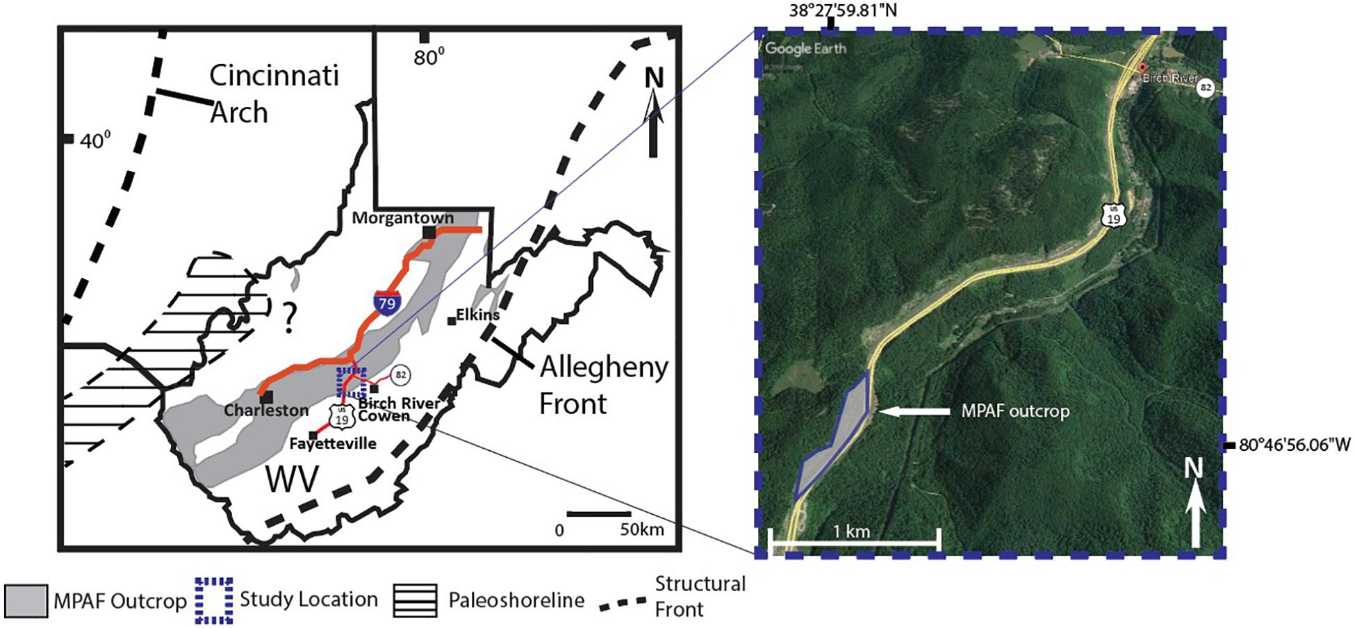
Figure 1. Study location, Birch River, West Virginia. The gray fill is the MPAF outcrop belt, WV. Dashed square is the outcrop location.

FIGURE 2

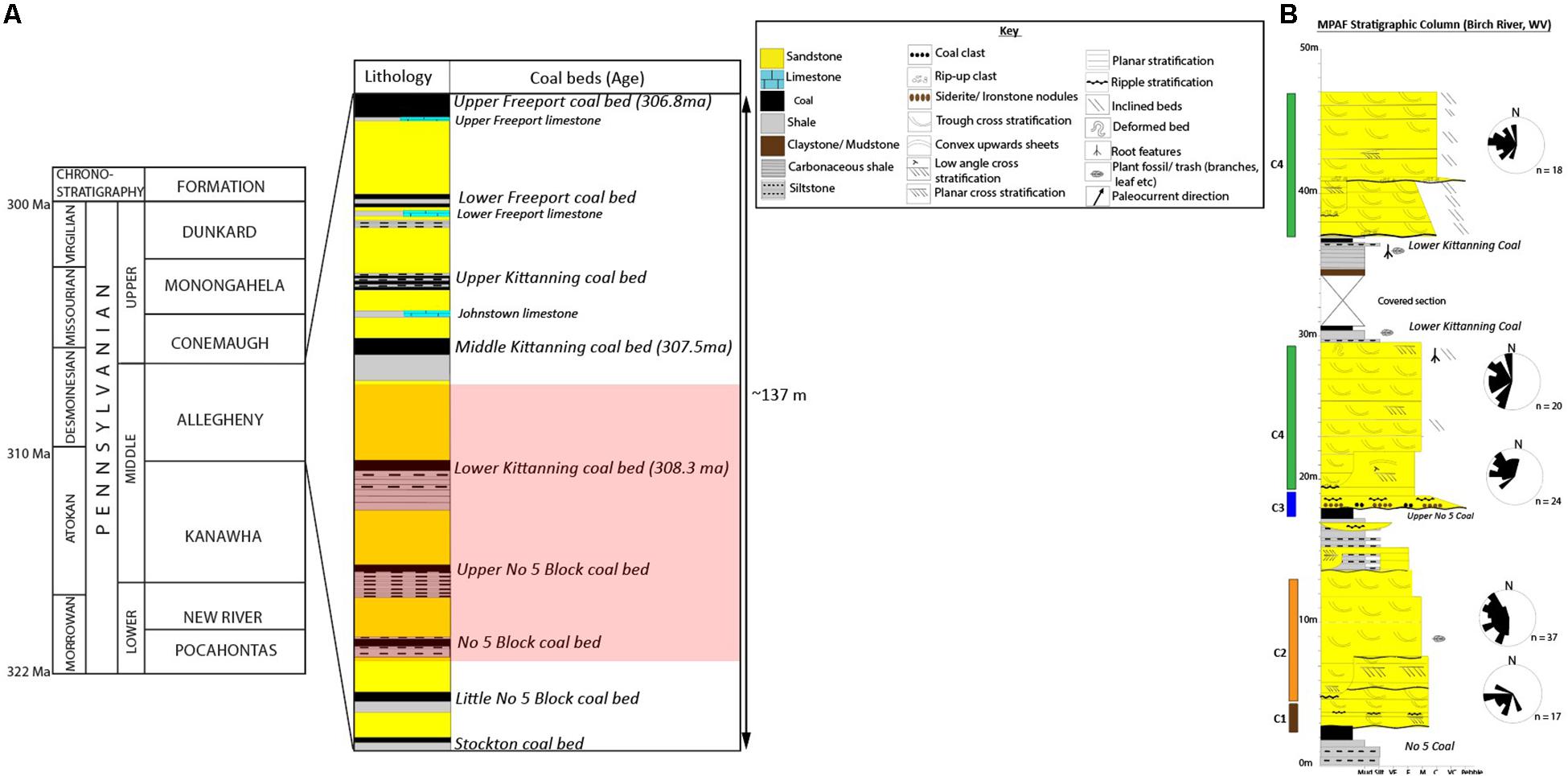
Figure 2. Chronostratigraphic column and lithostratigraphic column of the Middle Pennsylvanian Allegheny Formation (MPAF). (A) Chronostratigraphy of the lower MPAF study interval includes No. 5 Block, Upper No. 5 Block, and Lower Kittanning coal beds and associated clastic deposits (shaded square). Coal ages are reported in Montañez et al. (2016). (B) Lithostratigraphic column of the MPAF, Birch River, West Virginia. Modified from Blake et al. (2002) and Cecil et al. (2004). C is the channel belt and n is the number of paleocurrent measurements.

FIGURE 3

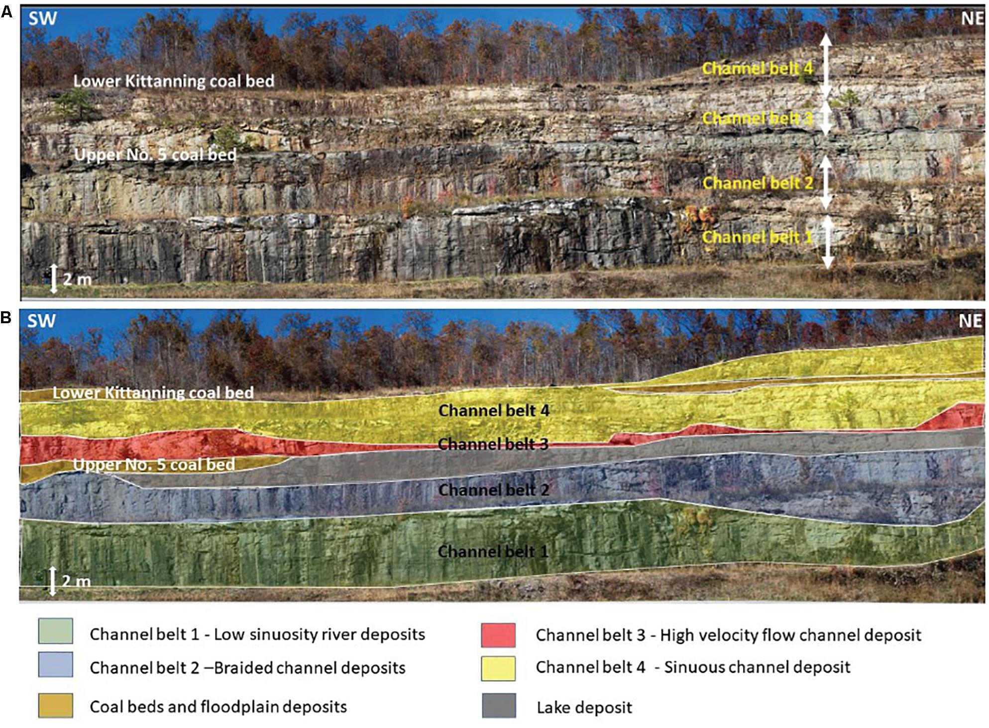
Figure 3. The Middle Pennsylvanian Allegheny Formation outcrop, Birch River, West Virginia. (A) Outcrop with scale (white bar), position of coal beds, and channel belt locations. (B) Birch River outcrop with interpreted channel belt boundaries.

Fluvial paleohydrology can be modeled from numerical equations based on grain size along with channel depth and width measurements and augmented by flow depth estimates from estimated dune bedform height (Ethridge and Schumm, 1977; Bridge and Tye, 2000; Leclair and Bridge, 2001; Leclair, 2002; Bhattacharya et al., 2016). These empirical equations relate sandstone grain size and channel geometry to estimates of paleohydrology. To build upon previous attempts at reconstructing paleohydrology of ancient fluvial systems, machine-assisted algorithms were developed to improve the accuracy of the estimated dune height from cross-set thickness using data of cross-set thickness and dune height from flume experiments reported by Leclair (2002) and Leclair and Bridge (2001). Multi-variate regression analysis was performed on the original data set to highlight the statistical significance (p-value) of the relationship between the variables in the data set. Support vector regression algorithm (herein and after referred to as SVR) was selected to better assess the relationship between variables with acceptable statistical significance (i.e., p-value < 0.05) because it can be used where bivariate relationships are established between geological properties with multivariate relationships (Ethridge and Schumm, 1977; Davis and Sampson, 1986; Bridge, 2009). Through this approach, the paleohydrological controls on MPAF fluvial architecture can be assessed to provide insights into the evolution of fluvial style and fluvial basin-fill record of the Alleghany foreland basin.

Geological Setting

Geologic History

The MPAF (Desmoinesian Stage, ∼310–306 Ma) is part of an Upper Paleozoic cratonward prograding clastic wedge shed from the adjacent orogenic highlands of the Allegheny orogeny during the late Middle Pennsylvanian (Arkle et al., 1979; Donaldson and Shumaker, 1981; Ettensohn, 2008). The collision of Laurasia and Gondwanaland (∼325 Ma) initiated the Alleghenian orogeny, which was characterized by collision and compressional deformation structures that formed the Allegheny fold-thrust belt (Donaldson and Shumaker, 1981; Ettensohn, 2005, 2008; Sak et al., 2012). The Alleghenian orogeny resulted in the formation of a broad shallower foreland basin than the Acadian and Taconic orogeny (Ettensohn, 2005, 2008). Paleoclimate models developed using coal beds, paleosol, soil carbonate-based, and fossil leaf-based proxies indicate that paleoclimate shifted from ever-wet humid to seasonally arid conditions during the Middle Pennsylvanian (Cecil et al., 2003, 2004; Tabor and Poulsen, 2008; DiMichele et al., 2010; Falcon-Lang and Dimichele, 2010; Montañez et al., 2016). In particular, palynomorph studies of the MPAF showed tree ferns, which are common in less humid environments, increased and became more common in No. 5 Block and Upper No. 5 Block coal beds sections of the MPAF, whereas lycopsids, which are common in very humid environments, dominated the LKC bed (Kosanke and Cecil, 1996; Eble, 2002; Falcon-Lang and Dimichele, 2010).

The major driver of the paleoclimate change was attributed to the low paleo-latitudinal position of the Appalachian Basin during Middle Pennsylvanian; and the effect of glacial volumes at the poles on Hadley Cell circulation patterns along the Intertropical Convergence Zone (ITCZ) (Cecil and Dulong, 2003; Cecil et al., 2004). Changes to the Haley Cell circulation patterns along the ITCZ resulted in the seasonality of rainfall in low latitudes during glacial minimum and high rainfall during glacial maximum. The development of a rain shadow on the Alleghenian foreland basin, which is located on the downwind side of the orogenic highlands, may have also contributed to the drier climate (Tabor and Montanez, 2002; Tabor and Poulsen, 2008). Paleobotanical and sedimentologic studies indicate that earlier MPAF depositional systems formed in a humid climate, while the MPAF above the LKC beds were deposited in a semi-arid climate (Cecil, 1990; Cecil et al., 2003; Greb et al., 2008; DiMichele et al., 2010; DiMichele, 2013; Montañez et al., 2016). Paleogeographic reconstructions of the North American craton suggest that the Appalachian basin was near the paleo-equator with Appalachian highlands to the northeast and coastal lowlands located to the west (Archer and Greb, 1995; Cecil et al., 2004). The resulting paleo-gradient resulted in south and western drainage directions (Donaldson and Shumaker, 1981; Cecil et al., 2003, 2004). Paleodrainage models based on sedimentary analysis indicate the MPAF clastic wedge is composed of swamp, lacustrine, fluvial, and deltaic deposits (Donaldson and Shumaker, 1981; Cecil, 1990). Marine fossils observed in MPAF sandstones suggest the downdip extent of the fluvial segments of the MPAF prograding clastic wedge is located in southeast Ohio (Stubbs, 2018).

MPAF Channel Belts, Birch River, WV

The MPAF clastic units are subdivided based on coal beds, which stratigraphically oldest to youngest include: No. 5 Block, Upper No. 5 Block, Lower Kittanning (No. 6 Block Coal), and Middle Kittanning coal beds (Arkle et al., 1979; Blake et al., 2002; Eble, 2002). Palynomorph studies found that more lysosomes (fungi) spores, which are common in humid ever-wet environment are more abundant in early Middle Pennsylvanian deposits below the MPAF, whereas herbaceous fern plants, which are common in less humid environments, were more abundant in late Middle to early Upper Pennsylvanian deposits (Cecil et al., 1985; Kosanke and Cecil, 1996; Peppers, 1996; Eble, 2002). Sedimentologic models used lithologic climate indicators such as presence of caliche, calcareous pedogenic concretions, and siderite to assess climatic fluctuations during the Pennsylvanian, including parts of the upper MPAF which includes the Middle Kittanning, Upper Kittanning, Lower Freeport, and Upper Freeport coal beds and their associated clastic deposits (Donaldson and Shumaker, 1981; Cecil et al., 1985; Cecil, 1990; Cecil and Dulong, 2003).

Materials and Methods

Facies Architecture of the MPAF Channel Belts

Facies associations and architecture were used to interpret the fluvial styles (Miall, 1996; Bridge, 2009). Facies and facies association were identified from a 45-m thick and 495-m wide outcrop (Miall, 1996; Bridge, 2009). Data were measured using a Wentworth calibrated grain-size card, measuring staff and ruler. Paleocurrent data were acquired from the left and right limbs of trough cross-strata using the best-fit circle method to determine paleocurrent direction on a stereographic plot (DeCelles et al., 1983).

Paleochannel Geometry Measurements and Estimation

Sedimentological data for the study was acquired from road cut (outcrop) along Route 19, Central West Virginia (Figures 1, 3). Units of MPAF present at Birch River outcrop include the No. 5 Block coal bed, the LKC bed, shale and sandstone units above and below No. 5 Block, the Upper No. 5 Block, and LKC coal beds (Blake et al., 2002; Eble, 2002; Cecil et al., 2004; Figures 1, 2). Sedimentologic data acquired from the outcrop include grain size, cross-bedding height, and barform height. These data were used to determine channel geometry (width and depth) by the methods outlined below.

Channel Depth

Channels were measured from preserved paleochannel boundaries corrected for compression during burial. Channel depths that were estimated from bar height involved the measurement of fully preserved channel bars in outcrop (Allen, 1970; Lin and Bhattacharya, 2017). The thickness of lateral or downstream accretion bars from outcrop, adjusted for 10% compaction factor, is representative of the bankfull channel depth (Ethridge and Schumm, 1977; Davidson and Hartley, 2010). The thickness of lateral or downstream accretion bars was determined using the fining upward sequence concept, where the lower and mid-section of the bar is characterized by planar, trough cross, planar cross, and inclined bedded sandstone that is relatively coarser than the upper section of the bar, which is characterized by massive and ripple bedded sandstone with plant debris and/or rooting structure (Bridge and Tye, 2000). The paleochannel flow depth was estimated from the thickness of lateral or downstream accretion macroforms using the equation by Ethridge and Schumm (1977):

$$d=D^{{}^{*}}/0.9(1)$$

where D^∗ is the maximum channel depth, which is represented by the thickness of the sandstone macroform, 0.9 compensates for the compaction factor. Errors associated with this method can be up to 100% if it is used for muddy sections (Holbrook and Wanas, 2014).

Channel depths were also estimated from dune-scale cross-set thickness, using empirical equations and machine-assisted algorithms. Previous work developed empirical equations which have been applied in the estimation of paleochannel dimension and morphology for ancient fluvial channel deposits. These equations determined relationships between the mean value of the exponential tail of the probability density function (PDF) for cross-set thicknesses and dune heights (Leclair and Bridge, 2001). The work by Leclair and Bridge (2001) has shown that the dune height (h_m) can be estimated from mean cross-set thickness (S_m) using a regression equation:

$$h_{\text{m}}=5.3\text{β}+0.001{\text{β}}^2(2)$$

$$\text{β}=S_{\text{m}}/1.8(3)$$

which can be simplified as:

$$h_{\text{m}}=\mathrm{\hspace{0.33em}2.9}{S}_{\text{m}}(4)$$

where h_m is the mean dune height, S_m is the mean cross-set thickness, β is the mean value of the exponential tail of the PDF for topographic height relative datum. The range of error in this empirical equation is ∼20% (Leclair and Bridge, 2001). Hence, the authors suggest the equation be used on data set with similar standard deviation. Based on the observation that the ratio of bankfull depth to dune height is common between 6 and 10 (Bridge and Mackey, 1993; Bridge and Tye, 2000), dune height (h_m) can be used to estimate channel bankfull flow depth (d):

$$6<d/h_{\text{m}}<10(5)$$

Machine-Assisted Estimation of Channel Belt

A support vector machine regression algorithm was developed to generate a new empirical equation that relates preserved cross-set thickness to dune height to improve channel depth estimates from cross-set thickness. These relationships were established from measurements of dunes, and corresponding cross-set geometry produced under known hydrological conditions of a flume. First, multiple regression analysis using least squares elimination method was applied to the data set of Leclair (2002), which includes measurements of flow conditions and resulting bedform and cross-set heights, in order to determine the statistical relationship between dune heights and cross-set thicknesses.

Multiple regression analysis

This study employs multiple regression to highlight the relationship between all the variables measured in flume studies that were used to explain the relationship between cross-set thickness and dune height (Leclair, 2002). The equation used for multiple regression is given as:

$$Y={\text{β}}_0+{\text{β}}_1{X}_1+{\text{β}}_2{X}_2+\mathrm{\cdots }+{\text{β}}_n{X}_n+\mathrm{\epsilon }(6)$$

where Y is the dependent variable represented as cross-set thickness, β₀ is the intercept, β_n are the coefficients, X_n are the independent variables describing flow conditions and depositional products, and ε is the random error. The accuracy of the multivariate regression was scored using R². Then, SVR was applied to create and improve empirical relationships between the variables with the highest level of statistical significance as determined from the multiple regression analysis.

SVR analysis

Support vector regression is a type of supervised machine learning algorithm that fits as many instances in the model by taking into consideration the outliers in the dataset while developing an empirical relationship. The SVR machine learning model was selected because it performs linear or non-linear regression in a higher-dimensional space using linear, polynomial, or Gaussian kernels. The kernels transform the data into a higher-dimensional space by creating a vector from the evaluation of the test positions of all the data and establishes a linear, polynomial, or Gaussian relationship among the variables in the data. The Gaussian kernel uses normal distribution curves around data points to try to establish a relationship with the variables being considered. The advantage of SVR over linear regression is that SVR allows the model to be less fitted to the training data but more flexible for predicting new data (Zhang et al., 2014). SVR can also be used for multivariate regression; hence, new variables can be added to try to improve predictions. The simplified equation for predicting the dependent variable (Y) using the SVR model (Bao and Liu, 2006; Awad and Khanna, 2015) is given by:

$$Y=w^T\mathrm{\varphi }(x)+b(7)$$

where Y is the dependent variable, w = (w₀, w₁, w₂,…)^T is the fitting coefficient in the higher dimensional space, ϕ is the kernel function transforming the independent variable x (cross-set thickness in this paper) to a higher dimensional feature space, and b is the intercept. The model’s performances compared to the previously used empirical equation (Eq. 2) were evaluated by testing the accuracy of the model’s predictions using mean square errors (MSEs). Grid search algorithm was used to determine the best penalty parameter (C), fitting error (ξ), and the kernel line of best fit for the data. Details of the algorithm and selected parameters to develop the SVR model are in the Supplementary Material. Algorithms for the SVR was written using Python and scikit-learn libraries (Pedregosa et al., 2011; Python, 2019). The steps taken to derive the SVR model for predicting dune height from cross set thickness include data preprocessing, kernel and parameter selection, and model fitting (Figure 4).

FIGURE 4

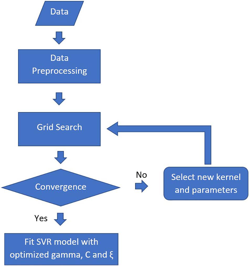
Figure 4. Workflow for support machine regression (SVR) analysis.

Data preprocessing

This includes sorting of the independent variable from lowest to highest value and normalizing the data. The cross-set thickness was set as the independent variable, while the dune height was set as the dependent variable for the SVR model. The cross-set thickness data were sorted and both data set were normalized. Normalization removes any disparity in the model that may be due to different units of measurements and large variance between values in the data that might skew the regression model in favor of the data set with larger values. The normalization of the independent and dependent variables involved adjusting both data set to a common scale. The normalization method used was MinMaxScaler, which has the ability to scale the data set between any range of values stipulated. The data were scaled into values between 0 and 1 using methods described in Pedregosa et al. (2011).

Kernel and parameter selection

Grid search was used to cross-check all kernels and parameters until there was convergence, i.e., the ideal kernel and parameters that will give the best solution are determined. Kernel is a weighing factor between two sequences of linear and/or non-linear data, which enables the correlation of the data set in higher dimension space (Pedregosa et al., 2011). Three types of kernel considered are linear, polynomial, and Gaussian kernels. The parameters considered include gamma, C, and epsilon (ξ). The gamma parameter defines how far the influence of a single training example reaches and can be seen as the inverse of the radius of influence of samples selected by the model as support vectors (Pedregosa et al., 2011). The gamma range considered was from 0.5 to 0.8. The C parameter trades off correct classification of training examples against maximization of the decision function’s margin; hence, the C parameter behaves as a regularization parameter in the SVM (Pedregosa et al., 2011). The range of C parameters considered was from 0.1 to 100. The epsilon defines a margin of tolerance where no penalty is given to errors (Pedregosa et al., 2011). The larger epsilon is, the larger errors you admit in your solution. The epsilon range considered was from 0.01 to 0.5. The gamma, C, and epsilon values, 0.8, 10, and 0.01, respectively, were selected because they produced the best SVR model. The accuracy of the SVR model, when using the Gaussian kernel and selected parameters 0.8, 10, and 0.01 for gamma, C, and epsilon values, respectively, is 84%.

SVR model fitting

Support vector regression model is fitted to the data set using the kernel and parameters from the grid search analysis. The model can be used to predict the dune height from cross-set thickness data inputted into the model. An inverse normalization is used to revert the normalized data and normalized model prediction.

Channel Width

Full channel widths were determined from Channel belt 1. Full channel belt widths could not be determined from the other channel belts because of the erosive nature of the channel boundaries. True channel width was derived from apparent channel widths measured from Channel belt 1 by correcting for the orientation of the MPAF outcrop and paleoflow direction. Channel width was also estimated using published scaling relationships for channel geometry that takes into consideration the channel style as well as the tectonic and climatic setting of the fluvial systems (Gibling, 2006; Blum et al., 2013). The common range of channel width to depth scaling ratios selected from Gibling (2006) includes 5–50 for fixed river systems, which were used in Channel belt 1, 50–1000 for braided and low-sinuosity rivers used for Channel belts 2 and 3, and 30–250 for Channel belt 4.

Paleoslope

Paleoslope was estimated using grain size and density of sediment grains following the empirical equation of Holbrook and Wanas (2014):

$${\text{τ}}_{\text{bf}50}^{{}^{*}}=(d_{\text{m}}S)/({\text{RD}}_{50})=\text{constant}(8)$$

where S is the slope, ${\text{τ}}_{\text{bf}50}^{{}^{*}}$ is the bankfull Shields number for dimensionless shear stress, d_m is the mean bank full flow depth, R is the submerged dimensionless density of sand–gravel sediment (qs–qw), and D₅₀ is the median grain size. ${\text{τ}}_{\text{bf}50}^{*}$ is assumed to be 1.86 after Holbrook and Wanas (2014).

Grain size for this study was quantified from thin-section petrography, as well as estimated from observations of rocks in outcrop using a grain size card with graphical representation of Wentworth grain size classes. The error in grain size made from grain size cards has an error of about 1/2 phi (Lin and Bhattacharya, 2017). Four thin sections were selected that were representative of average flow in the four fluvial channel types interpreted in the lower MPAF. The thin-sections were acquired from above the scour deposits, which should be representative of deposits of moderate flow conditions. For each thin section, the maximum axis of at least 100 grains was measured and used to calculate median grain size (D₅₀) for use in the empirical equation to estimate the paleoslope for MPAF paleochannels (Holbrook and Wanas, 2014).

Paleohydrology

Channel dimensions and paleoslope combined with flow velocity permit paleohydrologic reconstruction of MPAF channels using channel width derived from scaling factors so as to account for variabilities in channel cross-sectional area due to the depositional environment. Paleodischarge was estimated using the continuity equation (Eq. 9):

$$Q=\mathit{VA}(9)$$

where Q is the instantaneous discharge and A is the cross-section area, which is the product of channel width and depth. Flow velocity was estimated by using sedimentary structures to infer the bedform for comparison with the bedform phase diagram of Rubin and McCulloch (1980). The dominant bedform observed in the channel belts was used to estimate flow velocity under the assumption that the dominant bedform reflects dominant bedload transport conditions during flooding events (Bhattacharya et al., 2016; Lin and Bhattacharya, 2017). The cross-sectional area was derived from estimated depth using the SVR machine-assisted model and width from width to depth scaling the relationship of modern and ancient fluvial channels (Gibling, 2006). We elected to not use empirical equations to estimate channel width from channel depth estimates, as this approach does not consider channel style as a variable in constraining channel width.

Results

MPAF Channel Belts

Facies and facies architectural analysis revealed nine lithofacies that represented fluvial channel deposits. The channel lithofacies include horizontally stratified sandstone, ripple-stratified sandstone, poorly sorted sandstone, planar cross-stratified sandstone, trough cross-stratified sandstone, massive sandstone, and low angle cross-bedded sandstone or convex upward sandstone, laminated mudrock, and massive mudrock facies (Figure 5). The coal beds overlie mudrocks and non-channel sandstones. We categorize the fluvial channel deposits into channel belts based on the channel planform.

FIGURE 5

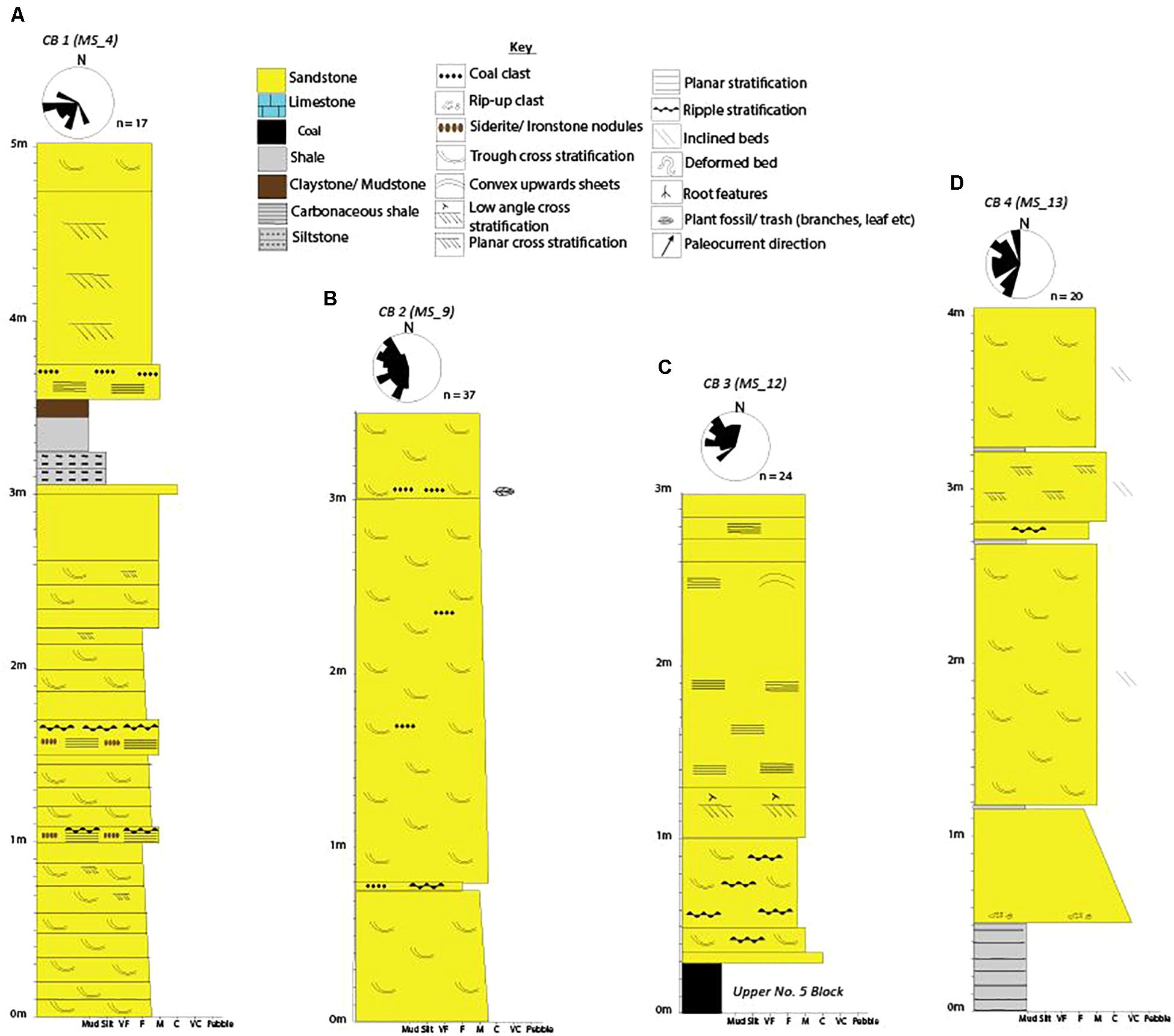
Figure 5. Measured sections of channel belts 1–4 showing key depositional facies and paleocurrent data. (A) Channel belt 1 (CB 1) represents low sinuosity channel deposits. (B) Channel belt 2 (CB 2) represents braided channel deposits. (C) Channel belt 3 (CB 3) represents high-velocity channel deposits. (D) Channel belt 4 (CB 4) represents sinuous channel deposits.

Channel Belt 1: Low Sinuosity Fluvial System

Channel belt 1 is made up of multiple stories up to 10-m thick of tabular and lenticular, fine to medium-grained sandstones with sharp, sub-horizontal to horizontal, undulating erosional basal contact and sharp, curved erosional bounding surface above (Figure 5). Channel belt 1 overlies the No. 5 Block coal bed (Figure 2). Five stories were identified in Channel belt 1. Individual stories are characterized by multiple sandstone bed sets, which may be capped by mudrock, and are bounded above and below by an erosional surface. The two bottom stories are made up to 3-m thick lenticular sandstone separated by a sharp near-horizontal erosional surface. The lenticular sandstones comprise of convex upward, fine to medium-grained, massive (Sm), and trough cross-stratified (St) sandstone with sharp, curved bedding plane at the base. The massive and trough cross-stratified sandstone beds are overlain by horizontal laminated sandstone (Sh) beds with a sharp horizontal bedding plane. The Sh is either onlaped by Sm or St beds with sharp, horizontal, or curved bedding planes. The Sm, St, and onlaped Sh beds are overlain by St and Sp beds with sharp horizontal bedding plane. The Sh may be overlain by interlaminated claystone, siltstone, and poorly sorted, ripple laminated sandstone in some places. The Sh may be overlain by interlaminated claystone, siltstone, and poorly sorted, ripple laminated sandstone in some places.

The three upper stories are made up of up to 2-m thick tabular sandstone bounded below by near-horizontal erosional surfaces. The tabular sandstones are made of tabular, fine to medium-grained trough cross and planar cross-stratified (Sp) sandstones with sharp, horizontal bedding plane. The Sp overlies the St in the tabular sandstone. The Sp may be overlain by horizontal laminated sandstone beds in some places. The Sp beds are up to 1-m thick in some places. The uppermost tabular sandstone is erosionally truncated and overlain by sandstones from Channel belt 2. The sandstone of Channel belt 1 contains abundant coal and siderite intraclast, and fossilized plant fragments. Channel belt 1 overlies the No. 5 Block coal bed. Paleocurrent data from trough cross-bedded sandstone indicate northeast to southwest direction of paleoflow. The lenticular sand bodies, which are overlain by Sh and onlaped by Sm and or St beds, are interpreted as mid-channel bar deposits while the tabular sand bodies are downstream accretion compound strata (Miall, 1996). The lack of a lateral accretion bar suggests low translation by channel. The abundance of coal and siderite intraclast suggest abundant vegetation and wet environment common in distal coastal plain depositional environments (Miall, 1996; Allen et al., 2014). Combined these features suggest Channel belt 1 are deposits of a distal, low sinuosity fluvial system.

Channel Belt 2: Braided Fluvial System

Channel belt 2 is made up of up to 5-m thick, multistory, amalgamated, medium-grained sandstone bounded above and below by sharp, undulating, horizontal, and curved erosional surfaces. Three stories were identified based on discontinuous, sub-horizontal, basal erosional surface, and channel lag deposits. Channel lag deposits, which comprise pebble size coal clast and iron-rich claystone clast and veins, were used to infer the base of the story where the basal erosional surfaces were not apparent. Individual stories are characterized by up to 0.3-m thick, amalgamated, medium-grained, compound through cross-stratified (St) sandstone beds with sharp or gradational, horizontal, or trough-shaped bedding plane. The St are rarely overlain by horizontal, fine-grained, ripple laminated sandstone (Sr) beds. Where the Sr is absent St may be overlain by up to 0.3-m thick, medium-grained, planar cross-stratified sandstone beds (Sp), or St. Channel belt 2 sandstones contain coal intraclast and petrified plant stems in places and is overlain by deltaic, lake, and well-drained floodplain deposits. The deltaic deposits are characterized by coarsening upward, interlaminated shale, and very fine-grained sandstone, the lake deposits are characterized by laterally continuous, tabular, massive sandstone beds, while the well-drained floodplain deposits characterized by discontinuous, lens-shaped, coarsening upward ripple laminated sandstone beds and laterally continuous interlaminated siltstone, mudstone, and shale, which are overlain by the Upper No. 5 Block coal bed. Paleocurrent data from the trough cross-stratified beds indicate both northwest and southwest paleoflow direction. However, the dominant paleoflow is toward the northwest. Neither lateral nor downstream accretion macroforms were observed in Channel belt 2. The abundance of compound trough cross-bedded facies suggests the system was dominated by 3D dunes. The presence of bed sets bounded by curved and/or horizontal bedding planes and the absence of a clear macroform such as lateral or downstream accreting deposits suggest that Channel belt 2 is dominated by compound bars common in braided channel fills (Miall, 1996; Bridge, 2009; Allen et al., 2014). Combined all these features lead to the interpretation of Channel belt 2 as deposits of a braided fluvial channel.

Channel Belt 3: High-Velocity Channel

Channel belt 3 is characterized by a fine to medium-grained, single-story tabular sandstone body bounded above and below by erosional surfaces. The facies association of Channel belt 3 is made up of poorly sorted, planar cross-stratified, trough cross stratified, massive, horizontally stratified, low angle cross stratified, and convex upward sandstone strata (Figure 5). This channel belt is composed of two distinct sandstone units: A lower unit dominated by interbedded poorly sorted and ripple bedded sandstone that is 0.5–1-m thick, and an upper unit dominated by sandstones with upper flow regime structures (Allen, 1982) such as horizontal and low angle cross stratified and convex upward sandstone (Miall, 1996; Fielding et al., 2009). In some areas, the lower sandstone unit has some trough cross-bedded facies at the base, which transitions abruptly into the poorly sorted ripple laminated facies locally. The low angle cross-stratified and convex upward facies are the most dominant bedform in this channel belt. Channel belt 3 overlies the Upper No. 5 Block coal bed. The abundance deposits with upper flow regime structures and the abrupt transition in facies succession suggest deposits by a high velocity flooding event therefore Channel belt 3 deposits may be deposits of a high velocity channel. The presence of low angle cross-beds and convex upward strata suggest supercritical flow event (Bridge, 2009; Allen et al., 2014; Miall, 2014). The presence of very coarse horizontal, ripple, and poorly sorted bedded sandstone is indicative of a fluvial system with substantial erosive power.

Channel Belt 4: Sinuous Meandering Channel

Channel belt 4 is characterized by fine to coarse-grained, multi-story inclined tabular and lenticular sandstone bodies bounded by sharp and erosional surfaces. A typical Channel belt 4 story is composed of poorly sorted sandstone, ripple stratified sandstone, planar cross-stratified sandstone, trough cross-stratified sandstone, and massive sandstone facies (Figure 5). Each story has poorly sorted and massive sandstone beds overlying an erosional base. The poorly sorted and massive sandstone beds are overlain by inclined, trough cross, and planar cross strata, which may be draped by ripple stratified sandstone locally. The sandstone bodies of Channel belt 4 stack vertically and extend laterally to form lateral accretion bars. The lower bounding surface for this channel belt is undulating erosional. The upper bounding surface is covered by soil and vegetation in the study area. Three stories were identified in the study location. The deposits of the first story of Channel belt 4 are overlain by floodplain deposits characterized by laterally continuous carbonaceous shale and claystone. The floodplain shale and claystone are overlain by the LKC bed. The Channel belt 4 sandstones below the LKC are deformed and have abundant root traces. The second and third stories do not have coal beds and are not deformed. The inclined geometry, vertical and lateral succession of massive, trough cross-stratified, planar cross-stratified, and ripple laminated facies are lateral accretion (point bar) deposits, which are common in the sinuous meandering channel. This led to the interpretation of Channel belt 4 sandstone bodies as deposits of a sinuous meandering fluvial channel system. The deformed sinuous channels were interpreted as water escape features caused by the oversaturation of the sinuous channel deposits (Plink-Björklund, 2015).

Machine-Assisted Approach to Dune Height Estimation From Cross-Bed Height

Multiple Regression

The machine-assisted model was developed using multiple regression analysis and the SVR algorithm on the flume experiment data used by Leclair and Bridge (2001) to derive the empirical equations. A p-value of 0.005 was selected to test the significance of the statistical relationship (Davis and Sampson, 1986). Backward elimination showed that dune height (h_m), as well as the dune length (lm) (i.e., the dune wavelength), had a high level of significance relationship (i.e., p-value < 0.005) with the cross-set thickness (S_m). It is difficult to measure the length of dunes in ancient deposits; hence, the relationship between cross-set thickness and dune height was further analyzed using SVR with the goal of developing a more efficient model for predicting dune height from the cross-set thickness in ancient channel deposits. These results from the multiple regression analysis highlighted the statistical relationship between cross-set thickness and dune height.

Support Vector Regression vs. Polynomial Regression

Dune height was set as the variable to be predicted from cross-set thickness (Figure 6) in order to compare SVR dune height predictions with the predictions from the empirical equation derived from polynomial regression (Eq. 4; Leclair and Bridge, 2001). The SVR model was used to predict dune heights from cross-set thicknesses derived from the flume experiment that Leclair and Bridge (2001) used to develop a polynomial regression model for dune height prediction from cross-set thickness. The Gaussian kernel, which used normal distribution analysis on data points in order to highlight the best-fitted hyperplane in the dune heights and cross set thicknesses regression plot, produced the best predictions in the SVR model. The MSE and root MSE (RMSE) were used to compare the accuracy of predictions from both methods. The RMSE of predicted mean dune height from using the Leclair and Bridge (2001) model (Eq. 5) was 16.8 mm, whereas the RMSE of predicted mean dune height from the SVR model was 9.3 mm, indicating the SVR model estimates were closer to the actual dune height produced in the flume experiment.

FIGURE 6

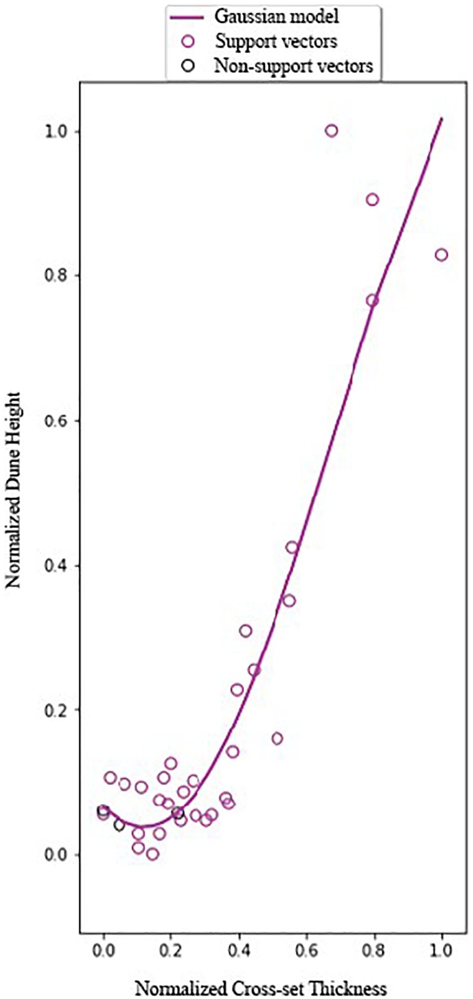
Figure 6. Variation of mean dune height (hm) and cross-set thickness (Sm), with a Gaussian kernel hyperplane. The support vectors are the data points used by the Gaussian kernel for plotting the best-fitted hyperplane for the regression analysis. Data sourced from Leclair (2002).

Paleochannel Depth Estimates

Paleochannel depth was estimated from measured bar thickness corrected for compaction in Channel belts 1 and 4 using Eq. 1; however, only incomplete channel bars were observed in Channel belts 2 and 3. Measurements of these incomplete bars were recorded to constrain minimum paleochannel depth (Table 1). Paleochannel depths estimates were also determined from dune heights predicted from cross-set thicknesses for all of the MPAF channel belts using Eq. 5 (Bridge and Tye, 2000; Tables 1, 2). Paleochannel depth was estimated from the dune height (h_m) based on the observation that the ratio of bankfull depth to dune height is commonly between 6 and 10 (Bridge and Mackey, 1993; Bridge and Tye, 2000). Paleochannel depth estimated from cross-set thickness was recorded for individual channel stories in Channel belts 1 and 4 (Table 2). Channel stories were not identified in Channel belts 2 and 3 because of the amalgamated nature of deposit from Channel belt 2 and the absence of channel stories in Channel belt 3. Overall, depth estimated from cross-set thickness measurements is greater than those estimated from bar thickness, suggesting that the bars of the MPAF have been largely subjected to substantial erosional truncation (Figure 7).

TABLE 1

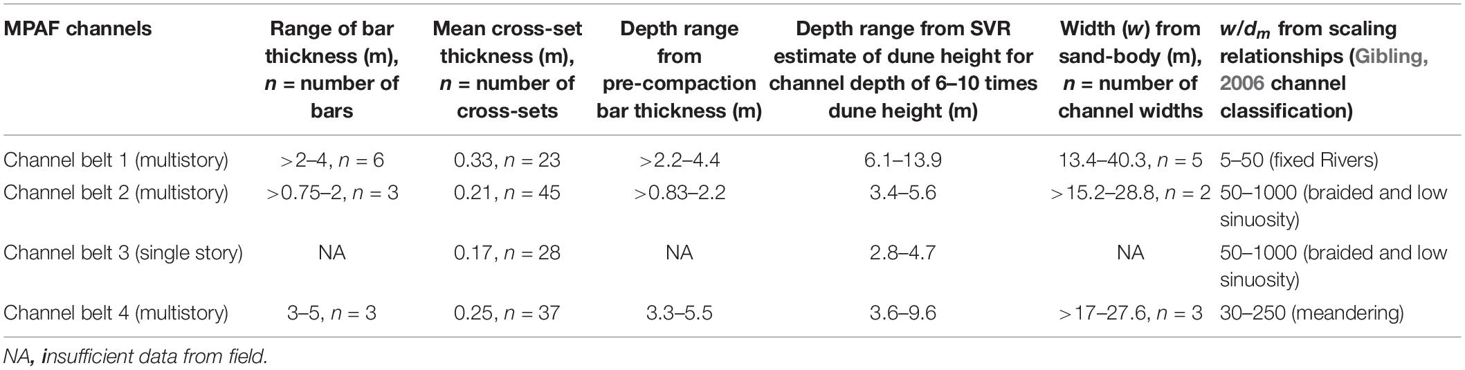
Table 1. Results of estimated paleochannel geometry.

TABLE 2

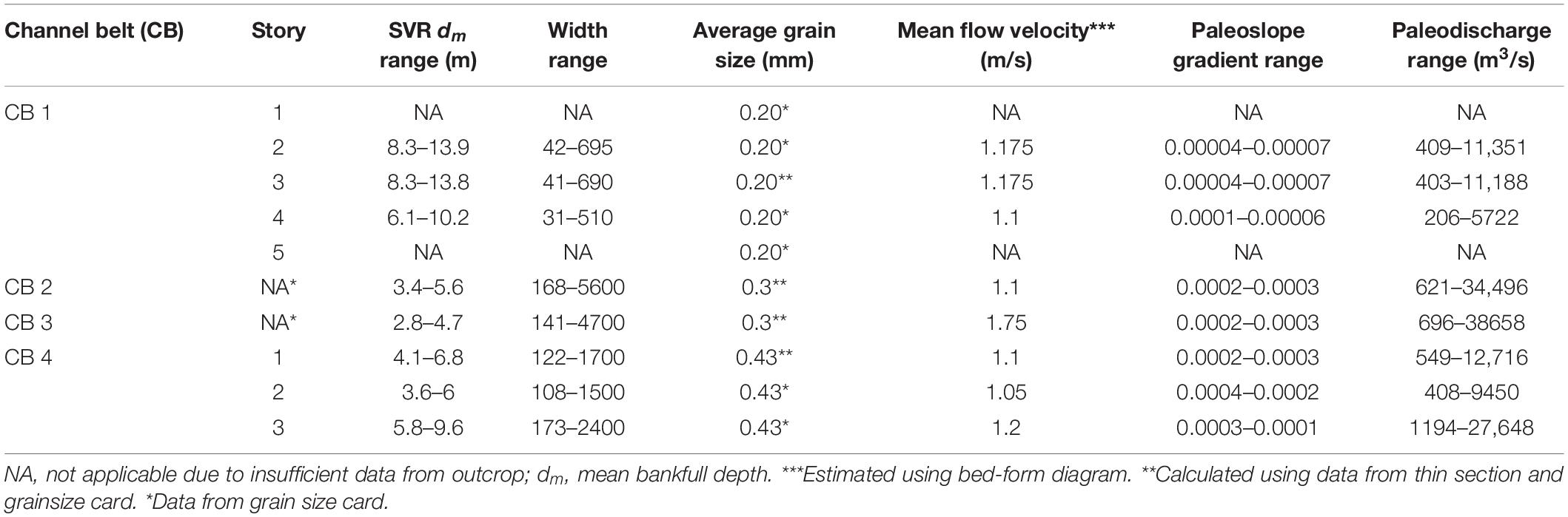
Table 2. Results of estimated paleogeometry (channel depth and width), paleoslope, and paleodischarge.

FIGURE 7

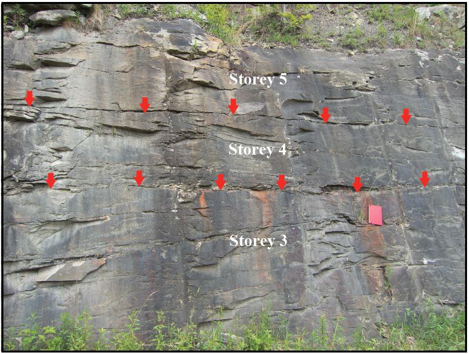
Figure 7. Channel belt 1 outcrop. Arrows highlighting truncation of channel bar deposits in Channel belt 1. Notebook is 25 cm long.

Bar thicknesses for Channel belt 1 were acquired from two channel bar deposits with a roll-over top, which is indicative of non-eroded channel bar deposits (Chamberlin and Hajek, 2015). The bar thickness was acquired from story 4 of Channel belt 1 using the same method as shown in Figure 8. The uncompacted thicknesses of these bars are 2.2 and 4.4 m. The bankfull paleochannel depths estimated from cross-set thicknesses using the SVR model were determined from measurements of 32 cross-set thicknesses. Depth estimates range from 6.1 to 13.9 m (Table 2).

FIGURE 8

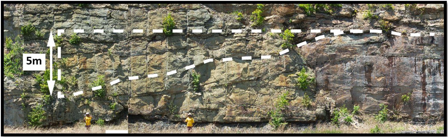
Figure 8. Example of how direct measurement of preserved bar is measured from outcrop data in Channel belt 4.

Depths could not be estimated from measured bar thicknesses for Channel belt 2 because of the compound nature of bars, erosional truncation, and partial preservation of the bar deposits. However, these partial bars can constrain minimum paleochannel to >0.83–2.2 m. The bankfull paleochannel depth estimated from the mean of 45 cross-set thicknesses ranges from 3.4 to 5.6 m.

Depths could not be determined from bar thickness for Channel belt 3 because of the lack of macroform scale sand bodies, which are used to interpret fluvial channel bars. Twenty-eight cross-set thicknesses were used to calculate the mean cross-set thicknesses used for SVR dune height prediction and paleochannel depth estimation. This yielded a depth estimate of 2.8–4.7 m.

Depth was estimated from bars with roll-over tops, which indicate they are fully preserved fluvial channel bar deposits (Figure 8; Chamberlin and Hajek, 2015). Bar thicknesses, which were measured from two bars in story 1 are 4.6 and 5.5 m, and one bar in story 2 of Channel belt 4 is 3.3 m. The bankfull paleochannel depth estimated from 37 cross-set thickness measurements from Channel belt 4 ranges from 3.6 to 9.6 m. The similarity in SVR predicted and bar thickness predicted bankfull paleochannel depths from stories 1 and 2 of Channel belt 4 indicates that Paleochannel depths predicted using SVR are accurate (Tables 1, 2).

Paleochannel Width Estimates

The apparent width of the channel boundaries were measured from the boundaries of incised channel deposits. The incised paleochannel widths represent minimum channel widths as the upper channel margins were commonly truncated. Channel widths were determined from nine sand bodies in the channel belts (Table 1). Apparent channel width was corrected for true width using paleocurrent direction. Paleocurrent direction was determined by 116 measurements of the orientation and dip of trough cross-beds. Measured channel width estimates range from values greater than the 13.4 to 40.3 m measured widths from the outcrop.

Channel widths were also estimated from the scaling relationships of channel width (w) to depth (d_m) ratio defined using modern systems by Gibling (2006). Estimated SVR channel depths were used to determine channel width. Channel width was estimated for individual stories in Channel belts 1 and 4 based on their interpreted channel styles. The paleochannel widths acquired from Channel belt 1 outcrop were from preserved channel boundaries, so the width was recorded as actual width. The paleochannel widths, which were determined from the measurement of five channel boundaries from Channel belt 1 deposits, are up to 40.3 m (Table 1). The measured paleochannel widths determined from the deposits of Channel belt 1 fall within the channel width ranges determined from the scaling relationship. The width range determined from the scaling relationship is 31–695 m (Table 2). The width was determined by using the minimum and maximum w/d of 5 and 50, and SVR bankfull flow depth estimates of 6.1–13.9 m (Tables 1, 2). The common w/d ratios for fixed channels in distal humid environments (Gibling, 2006) were used for widths analysis in Channel belt 1.

The measured paleochannel widths of the fluvial channel incision from Channel belt 2 are 15.2 and 28.28 m (Table 1). Two instances of channel incision were observed in Channel belt 2. The deposits of the incised channel were eroded therefore the upper boundaries of the paleochannels could not be determined. The w/d scaling relationship of 50–1000 for braided fluvial channels (Gibling, 2006) and mean flow depths estimated from the SVR were used for estimating widths for Channel belt 2. The paleochannel width range derived from w/d scaling relationship is 168–5600 m (Table 2).

Channel belt 3 does not have enough sedimentary features to determine channel width. It was difficult to measure any form of channel boundaries because deposits of Channel belt 3 did not have macroforms such as channel bars that could be used in identifying channel boundaries. The w/d scaling relationship of 50–1000, for braided and low sinuosity fluvial channels (Gibling, 2006) and mean flow depths estimated from the SVR were used for width estimate in channel belt 3. The paleochannel width range derived from w/d scaling relationship is 141–4700 m (Table 2).

The paleochannel incision widths measured from channel belt 4 are up to 27.6 m (Table 1). There were three instances of channel incision in Channel belt 4. The deposits in the channel incision were also eroded at the upper section, which made it impossible to estimate the true channel widths. The w/d scaling relationship of 30–250, for meandering fluvial channels (Gibling, 2006) were used for estimating widths in Channel belt 4. The paleochannel width range derived from w/d scaling relationship is 108–2400 m (Table 2).

Paleoslope Estimation

The paleoslope was estimated using grain size determined from thin-section petrography and a grain size card with a graphical representation of Wentworth grain size classes (grain size table in Channel Paleohydrology Supplementary Material). The overall grain sizes of the MPAF channels deposits range from pebble to clay sizes, which is common in fluvial channel deposits (Table 2). The clastic sediment of the MPAF fluvial channels are moderately sorted. The sediment grain sizes of Channel belt 1 ranges from coarse to fine-grained sand (0.5–0.17 mm) with the fine to medium-grained sand (∼0.25 mm) being the most dominant mode. The grain sizes of Channel belt 1 from thin section analysis yielded a D₅₀ grain size value of 0.23 mm, categorized as fine-grained sandstone. The sediment grain sizes of Channel belt 2 vary from coarse to fine-grained sand (0.1–1.05 mm). Thin section analysis of Channel belt 2 resulted in a D₅₀ grain size value of 0.33 mm, categorized as medium-grained sandstone. Channel belt 3 has sediment that varies from pebble to medium-grained sand (>2–0.25 mm). The D₅₀ value of Channel belt 3 is 0.3 mm, categorized as medium-grained sandstone. Channel belt 4 sediment clast size varies from pebble to mud (>2 to <0.088 mm). Channel belt 4 grains have a D₅₀ value of 0.4 mm, categorized as medium-grained sandstone.

Paleoslope of the MPAF channels estimated using Eq. 8 ranges from 0.00007 to 0.0004 (Table 2), which suggests a low paleoslope comparable to slope ranges for the Amazon, Mississippi and Niger Rivers (slope range ∼0.00002–0.0005; Blum et al., 2013). The estimated paleoslope for Channel belt 1 0.00007–0.0001. The estimated paleoslope for the other channels are: Channel belt 2 are 0.0002–0.0003, Channel belt 3 are 0.0002–0.0003, and Channel belt 4 are 0.0001–0.0004, which are an order of magnitude steeper than the estimated slope of the low sinuosity channel. The estimated lowest slope for Channel belt 1 agrees with the dominant fine grain size observed in the sand body.

Paleohydrology

The MPAF channel belt flow velocities, which were estimated using the bedform phase diagram, ranges from 0.6 to 2 m/s (Figure 9 and Table 2). The flow velocity of Channel belt 1 is in the range of 0.85–1.5 m/s. The estimated flow velocity of Channel belt 1 was determined by using the bankfull depth range of 6.1–13.9 m, the dominant sedimentary structure, which is trough cross-stratification produced by dune bedforms, and the fine-grained sand bed form diagram. The estimated flow velocity of Channel belt 2 ranges from 0.6 to 1.6 m/s. The flow velocity of Channel belt 2 was determined using the bankfull depth range of 3.4–5.6 m, and plotting the chart area for the dominant sedimentary structure, which is dune scale cross-sets, on the medium-grained sand bedform phase diagram. Channel belt 3 deposits are dominated by lamination produced from low-amplitude, upper flow regime bedform; therefore, the bankfull depth range of 2.8–4.7 m was used to estimate a velocity range of 1.5–2 m/s. The velocity of Channel belt 4 was determined using the dominant sedimentary structure, which is the dune-scale cross-sets and the estimated channel depth range of 3.6–9.6 m to estimate the velocity, which ranges from 0.6000 to 1.7 m/s. Paleodischarge for the channel belts range from 206 to 38658 m³/s. Channel belts 2 and 3 with paleodischarge values of 621–34,496 and 695–38,658 m³/s are the highest paleodischarge. The other paleodischarge ranges are 206–11351 m³/s for Channel belt 1 and 408 to 27648 m³/s for Channel belt 4 (Table 2).

FIGURE 9

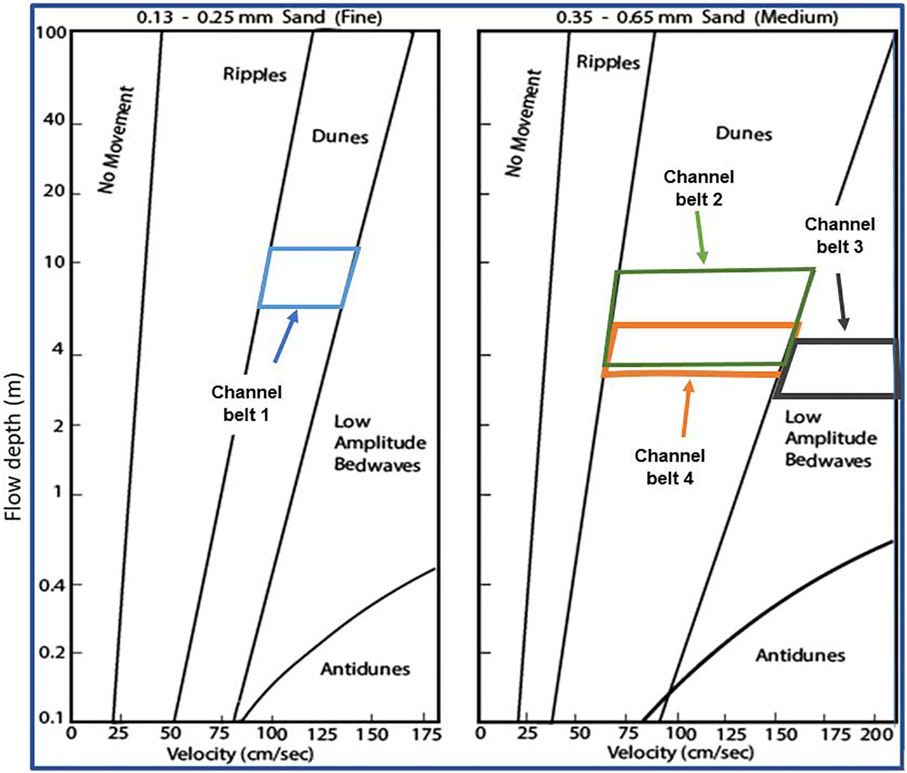
Figure 9. Fine and medium-grained bedform phase diagrams of Rubin and McCulloch (1980). Estimated range of velocity for Channel belt 1 is 85–145 cm/s, Channel belt 2 is 6000–16,000 cm/s, Channel belt 3 is 150–200 cm/s, and Channel belt 4 is 6000–170 cm/s.

Errors and Uncertainties Associated With Numerical Analysis

Measurement of channel fill structures in the outcrop is subject to bias in interpretation sedimentary features from outcrop data, which represents an initial source of error. Detailed architectural analysis of outcrop aided the identification of channel bar (Bridge, 2009; Holbrook and Wanas, 2014). Other problems associated with measuring thickness data from channel bar include compaction and erosion. The degree of compaction is dependent on several factors such as original packing, original void ratio, shape of grains, degree of roundness of grains sand composition, and size grading (Ethridge and Schumm, 1977). Equation 1, which takes into account factors that affect the degree of compaction, was used to compensate for the 10% error due in measured bar thickness to compaction. It is impossible to estimate channel depth from an eroded bar; hence, data from eroded bar were recorded to give a minimum estimate of channel bar thickness. Errors associated with identifying and measuring channel bars can be up to 60% (Holbrook and Wanas, 2014). Errors identifying channel bar thickness using story thicknesses can be up to 25% (Holbrook and Wanas, 2014). Mean channel depth estimated from cross-set thickness is subject to the bias of preferential preservation of dunes during waning flow, which may not be representative of actual bankfull flow. This results in the estimation of mean dune heights that are not representative of actual flow conditions, which cause errors in the depth estimates. Mean channel depth estimated from dune height and cross-set thickness by using Eq. 5 have errors up to 25% if the depth range is averaged (Holbrook and Wanas, 2014). The accuracy of dune heights estimated using SVR is 84%. The score was calculated using the coefficient of R². Errors associated with estimating channel depth with Eq. 5 will also be encountered (Pedregosa et al., 2011). Measurement of channel width is also subject to the bias of interpretation, which may lead to errors in data acquired. Accuracy of channel width measurement is dependent on the identification of channel banks, which proved to be extremely difficult in the study outcrop. Channel width estimated form scaling factors have error ranges by a factor of ±4 (Blum et al., 2013). Channel dept and width estimated from the rock record are representative of extreme events, which may have resulted in extreme geomorphology and discharge than is normal to the depositional system (Gibling, 2006). Error associated with slope estimates is the assumption that bed shear stress required to move the sediment load is constant across the channel. The bankfull shield number used as a constant is for slope estimation varies by ±2 (Holbrook and Wanas, 2014). The grain size used for estimating slope is an average value and was measured with a Wentworth grain size calibrated card, which has errors of ∼1/2 phi (Lin and Bhattacharya, 2017). The errors associated with paleodischarge estimates are up to an order of magnitude (Holbrook and Wanas, 2014; Lin and Bhattacharya, 2017). The instantaneous paleodischarge estimates are not representative of the annual or seasonal discharge in the paleochannel. The instantaneous discharge equation is a function of velocity of bankfull floodwaters, cross-sectional area of a channel, assuming the sediment supply is constant. The assumption of constant sediment supply adds more errors to the paleodischarge estimates as sediment type and sediment load varies. Another error associated with the paleodischarge estimate is based on the assumption that the cross-sectional area of a channel is the same, which is not so (Holbrook and Wanas, 2014). The cross-sectional area was also calculated using depth and width estimates, which means the errors from those numerical estimates are reflected in paleodischarge estimates. Additionally, the estimates from the instantaneous discharge have errors because the cross-sectional area for the paleochannels is estimated from mostly eroded channel deposits, which may not be representative of the actual sediment load.

Discussion

Machine-Assisted Paleohydrological Analysis

The machine-assisted SVR analysis increased the accuracy of dune height prediction from cross-set thickness resulting in a higher accuracy of estimated channel depth. The results of the SVR analysis were compared to the widely used polynomial regression model developed by Leclair and Bridge (2001) using MSE and overall predictions showed comparable and in most cases better performance. The result from MSE analysis showed that the SVR model had a RMSE of 9 mm while the polynomial model had an RMSE of 16.8 mm.

Advantages of SVR Over Polynomial Regression

The SVR model considers outlier data when estimating dune cross-strata thickness. Furthermore, SVR analysis is done in a higher dimension so it allows for a comparison of additional variables that may improve prediction. For example, cross-set length may be added to the SVR model to improve the accuracy of predicted dune height. In geology, all data are important because they reflect the variability of the conditions during bed formation. The model of Leclair and Bridge (2001) was based on the data along the best line of fit. The predictions of the SVR model are non-linear due to the use of the Gaussian kernel, i.e., the model uses normal distribution to predict the zone of best fit. The result of utilizing outlier data and the Gaussian kernel is a more accurate prediction as evident by the RMSE of SVR compared to the previous model.

Channel Belt Evolution

Facies architecture, channel dimensions, paleoslope, and paleodischarge of the MPAF channel belts reveal an evolution of fluvial channel form in response to changing paleohydrological conditions. Of note, the channel depth shows variability among MPAF channels: 6.1–13.9 m for Channel belt 1, 3.4–5.6 m for Channel belt 2, 2.8–4.7 m for Channel belt 3, and 3.6–9.6 m for Channel belt 4. Channel width estimated from scaling relationships showed that the low sinuosity channels had a lower range of width, while the braided channels had the largest width range. The independently estimated paleoslope and paleodischarge, which were compared among the MPAF channel belts (Table 2), showed that all the channel belts at the study location had a low slope (0.00007–0.0004) and variable paleodischarge (Figure 10). The estimated paleoslope of the lower MPAF channel belts is similar to slope ranges for the Amazon, Mississippi, and Niger Rivers (slope range ∼0.00002–0.0005; Blum et al., 2013). This indicates that the paleoslope estimates obtained for the MPAF fluvial systems are consistent with physiographic models that suggest MPAF were deposited in low-gradient environments caused by unloading type relaxation of the foreland basin (Cecil, 1990; Cecil et al., 2003; Greb et al., 2008). Given the relatively low paleoslope estimated for all MPAF channel belt, the formation of upper plane beds and low amplitude bedforms from high-velocity flow is considered to reflect flooding events caused by intense precipitation (Kosanke and Cecil, 1996; Miall, 1996, 2014; Cecil and Dulong, 2003; Cecil et al., 2003).

FIGURE 10

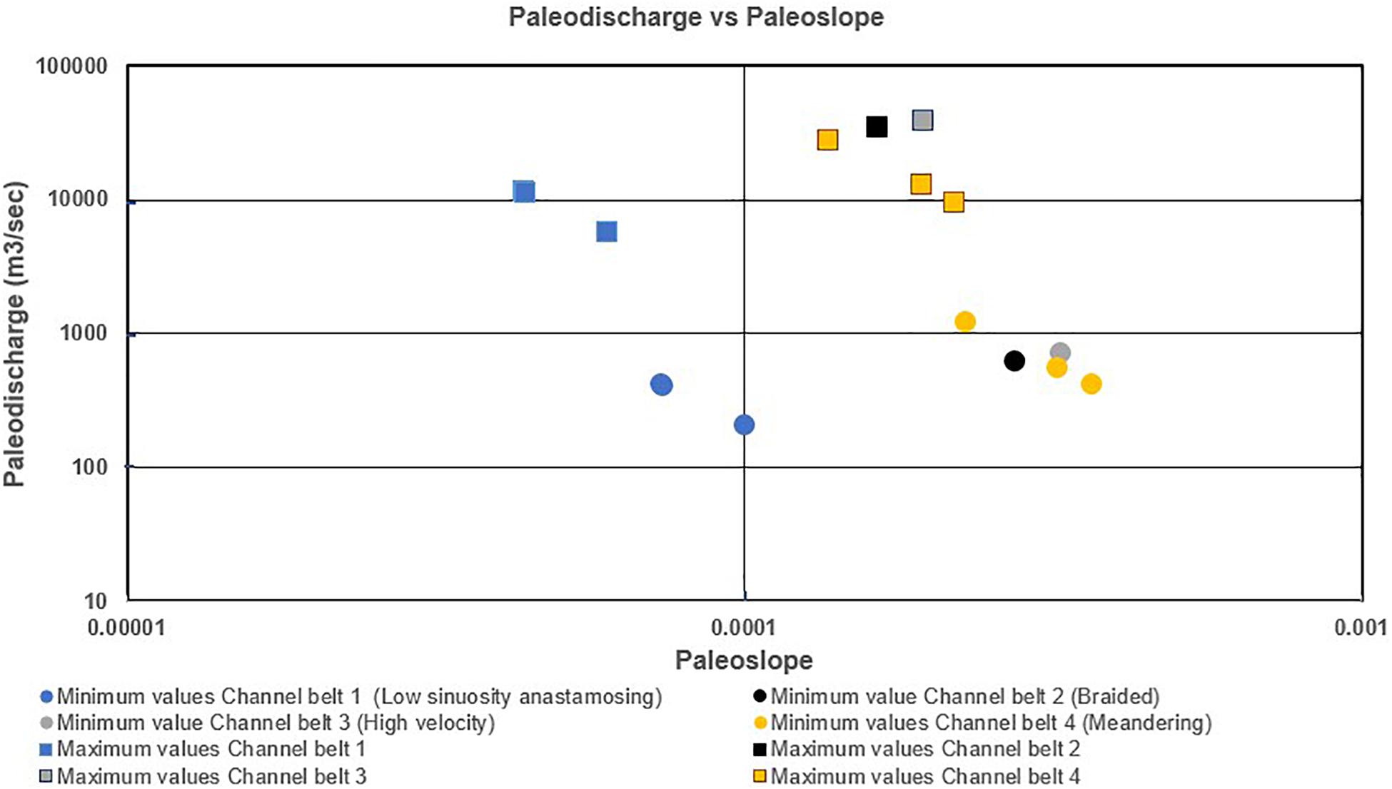
Figure 10. Plot of paleodischarge versus paleoslope of MPAF channels at Birch River, WV.

Results indicate Channel belt 1 deposits formed from a low gradient, fine-grained, low-sinuosity channel form in an anastomosing fluvial system. Channel belt 1 has the thickest channel depth (6.1–13.9 m), which results in a relatively low w/d. This low w/d combined with the grain size, slope, and an abundance of coal intraclast and large plant fragments may reflect channel confinement due to bank stabilization by vegetation. The abundance of coal intraclasts and large plant fragments suggests abundant vegetation, which flourished in the humid climate, surrounded areas in the low sinuosity fluvial system (Cecil, 1990; Cecil et al., 2003; Allen et al., 2014). The estimated range for the paleoslope of the low-sinuosity channel of 0.00007–0.0001 is an order of magnitude lower than other MPAF channels in the study area. The low slope and high amount of fine-grained deposits may have contributed to Chanel belt 1 having the relatively highest channel depth and a low w/d (Gibling, 2006). The estimated paleodischarge for Channel belt 1 is 206–11351 m³/s. This range of paleodischarge rate is the lowest of all the MPAF channel belts in the study area and is consistent with the abundance of fine-grained sediments deposited (Figure 10; Miall, 1996, 2014; Catuneanu, 2006).

Channel belt 2 directly overlies Channel belt 1 (Figures 2, 3) and contains features that indicate deposition by a braided fluvial system in a humid climate, with low channel confinement, low paleoslope, and high paleodischarge. Channel belt 2 deposits are characterized by an abundance of trough cross-stratified, medium-grained sand, with a paleochannel depth range of 3.4–5.6 m. The abundance of trough cross-stratification suggests that the channel system was dominated by 3D dunes. The low paleochannel depth, higher slope values (0.0002–0.0003) and higher paleodischarge (621–34496 m³/s) compared to other MPAF channel belts (Figure 10), suggests that the braided channel style of Channel belt 2 is due to mainly to an increased slope gradient. Channel belt 2 is interbedded with some plant trunk and coal clast, which suggests an abundance of vegetative material in the fluvial system; this suggests that the area was vegetated, but this vegetation wasn’t sufficient for bank stabilization.

Overlying the No. 5 block coal bed (Figures 2, 3), Channel belt 3 sandstones were deposited by a low gradient, high-velocity fluvial system in a seasonal semi-arid climate. Channel belt 3 is characterized by an abundance of medium-grained, low amplitude bedforms and a relatively high width to depth ratio. The abundance of low amplitude bedforms in Channel belt 3 was attributed to high-velocity flooding event(s), which is supported by high paleodischarge values (695–38,658 m³/s) compared to other MPAF channel belts. Channel belt 3 exhibits the shallowest paleochannel depths estimates compared to the other MPAF channels. This combined with the low paleoslope for Channel belt 3 (0.0002–0.0003) suggests that high-velocity flow resulted from a control other than paleoslope (Cecil et al., 2003; Cecil and Dulong, 2003; Plink-Björklund, 2015). The Burdekin River is an analog system developed in a seasonally wet-dry climate that experiences high velocity flows due to monsoonal precipitation events during wet seasons (Fielding and Alexander, 1996). The Burdekin River, just like CB 3, is dominated by upper plane beds and dunes, which represent fluctuating periods of extreme and moderate flow events.

Channel belt 4 directly overlies Channel belt 3 and contains features that indicate deposition by a low-gradient sinuous fluvial system. The high-velocity channel (Channel belt 3) is overlain by Story 1 of the sinuous channel (Channel belt 4). Story 1 is characterized by coarse to medium-grained, inclined sandstone beds with a channel depth range of 4.1–6.8 m (Table 2). The occurrence of convoluted beds and root structures in story 1 of the sinuous fluvial system may have been due to changes in water levels of the fluvial system brought about by seasonality in rainfall due to increasing aridity (Cecil et al., 2003; Cecil and Dulong, 2003; Fielding et al., 2009; Allen et al., 2014; Plink-Björklund, 2015). Overlying Story 1 is the LKC bed, which is overlain by Stories 2 and 3. Stories 2 and 3 are characterized by coarse to medium-grained, inclined sandstone beds with a channel depth range of 3.6–9.6 m (Table 2). The paleoslope (0.0001–0.0004) and paleodischarge (408–27,648 m³/s) values of Channel belt 4 indicate an order of magnitude increase in the maximum paleodischarge rate despite the low channel gradient.

The effect of paleochannel geometry, paleoslope, and paleohydrology on the fluvial channel architecture and depositional style of the MPAF varies. The geometry of the MPAF channel varies in the study area. The channel width and depth, which has been used to compare fluvial channels of arid to humid differing climatic regimes (Fielding et al., 2009; Allen et al., 2014), was used to compare the MPAF channels. The depth ranges for the MPAF channels showed variability among MPAF channel belts: 6.1–13.9 m for Channel belt 1, 3.4–5.6 m for Channel belt 2, 2.8–4.7 m for Channel belt 3, and 3.6–9.6 m for Channel belt 4. The independently estimated paleoslope and paleohydrology, which were compared among the MPAF channel belts (Table 2 and Figure 10), showed that the variation in channel depth of all the channel belts at the study location had developed on a low slope and with variable paleodischarge (Table 2 and Figure 10). The low paleoslope observed in all MPAF channel belt also indicates that fast-flowing events that resulted in the formation of upper plane beds and low amplitude bedforms may have been due to flooding events caused by fluctuation in precipitation intensity (Kosanke and Cecil, 1996; Cecil et al., 2003; Cecil and Dulong, 2003; Miall, 2014).

Possible Controls on Fluvial Channel Geometry and Paleohydrology

Eustatic rise and fall of sea level may have controlled paleoslope by changing fluvial base level (Blum and Törnqvist, 2000) across the basin in which a reduction in fluvial gradient due to sea-level rise should result in a reduction of channel flow velocity, while an increase in fluvial gradient should increase channel flow velocity. Glacio-eustatic models suggest fluvial channel sandstones are mainly deposited during glaciation when base-level is low in the basin and floodplain mudrocks are deposited during interglacial periods, when the base-level is high (Falcon-Lang, 2004; Greb et al., 2008; Haq and Schutter, 2008; Falcon-Lang and Dimichele, 2010). The effects of base-level rise and fall have a direct influence on the water levels and hence the flow depth of the fluvial channel. Sediment accommodation in a fluvial channel is limited by the water level and this is reflected in the thickness of preserved channel sand bodies of the MPAF (Shanley and McCabe, 1994; Currie, 1997; Blum and Törnqvist, 2000; Bhattacharya et al., 2016). The thicker channel depth observed in CB 1 and CB 4 may be due to eustatic base-level rise, while the lower thickness values of CB 2 and CB 4 may be due to eustatic base-level fall. However, the occurrence of water escape structures and rooting features in CB 4 sandstones suggests a variable water level in the fluvial system, which is not consistent with the eustatic base-level fluctuations. This suggests that glacio-eustasy played an important role in long-term accommodation succession of the fluvial system, but other factors overprinted the glacio-eustatic control.

Tectonic controls on accommodation and physiography of the Alleghenian foreland may have affected the evolution of MPAF channel belts. Tectonic subsidence and uplift may lead to the increase or decrease of slope and hence fluvial gradient. Relaxation and uplift of a subsided Alleghenian foreland basin would have resulted in an increase of slope (Holbrook and Schumm, 1999; Holbrook et al., 2006), which we interpret to have caused an increase of the fluvial gradient and change in fluvial styles reflected in the CBs 1–3 (Table 2). The effect of tectonic subsidence and uplift on the base level is similar to the eustatic effect on base level in a sedimentary basin. However, tectonic processes have third-order cycles (i.e., >1 my) which do not fit the higher frequency, fourth-order cycles (i.e., 0.1–1 my) of the MPAF channel belt (see MPAF age estimates, Figure 2). This implies that tectonic influence on MPAF geometry and paleohydrology has been masked by other controls. Additionally, tectonic uplifts which resulted in the formation of the Pangean Mountains may have resulted in the formation of a rainshadow zone, which led to extended periods without precipitation (Greb et al., 2008). However, the duration of tectonic processes does not match the higher frequency processes of the MPAF (DiMichele et al., 2010; Gibling et al., 2014).

Paleoclimatic control on precipitation and evapotranspiration rates and the abundance of vegetation may have influenced the geometry and hydrology of the MPAF fluvial system. An increase in or decrease in annual precipitation and evapotranspiration rates may have led to changes in the rate of discharge in the catchment area and fluvial system. The abundance of vegetation in different climatic conditions may also affect the geometry and hydrology of the fluvial system. The amount of vegetative cover influences the run-off in a fluvial catchment area and rooting increases the stability of channel banks (Schumm, 1968, 1981, 1988; Fielding et al., 2009). The amount of vegetative cover in the fluvial catchment area of ever-wet, humid fluvial systems have more vegetative cover and experience less erosion and water run-off compared to more arid catchment areas with less vegetative cover. Precipitation and evapotranspiration rates also vary in fluvial systems of humid and seasonally wet–dry climates (Cecil and Dulong, 2003; Cecil et al., 2004). The constant precipitation events and abundant vegetation cover in the fluvial depositional system of an ever-wet humid climate results in stable water input in the fluvial catchment area and constant paleodischarge rates in the fluvial system. Any fluctuation in the base level of the ever wet, humid fluvial system is driven by other factors such as eustasy. Also, erosion in the humid fluvial system will be limited to areas within the channel due to the stabilizing effects of abundant vegetation on the channel banks, which may lead to increased channel flow depth compared to channel width. The increased thicknesses of Channel belts 1 and 4 deposits above the LKC may be due to deposition in a humid climate characterized by constant precipitation, an abundance of vegetation and moderate paleodischarge. The sinuous channel belt (CB 4) and the low sinuosity channel belt (CB 1) have the lowest range of paleoslope and paleodischarge, except for the uniquely high paleodischarge range of the story 3 of the sinuous channel belt, which may be due to an increase in base level as a result of an increase in precipitation rates. Fluvial systems of seasonally wet–dry climates experience more evapotranspiration, which results in a reduction in water levels in the fluvial system. Precipitation events in the fluvial systems of seasonally wet–dry climates result in a sudden increase in water input to the fluvial catchment area, which results in increased paleoflow and paleodischarge (Cecil and Dulong, 2003; Fielding et al., 2009; Plink-Björklund, 2015). The relatively low thickness of the braided and high-velocity channel suggests that there was low accommodation, which may be due to the reduction of the stratigraphic base level during the periods of high evapotranspiration. The high range of paleodischarge values of the braided (CB 2) and high-velocity (CB 3) channel belts indicates a high paleoslope and fluvial gradient, which may have been due to onset of precipitation in a fluvial system previously experiencing low stratigraphic base level, which we interpret to have been caused by high evapotranspiration rates during dry season.

Paleoclimatic models developed from miospore composition of coal indicate wet–dry–wet MPAF depositional environment (Figure 11; Eble, 2002), which was attributed to fluctuations in paleoclimate of the Appalachian basin during the Middle Pennsylvanian (Eble, 2002; DiMichele et al., 2010; Falcon-Lang and Dimichele, 2010; Cecil, 2013). The miospore data show lycopsid, fern, calamites, and cordaites composition of MPAF coal beds at Birch River. The lycopsid indicates deposition in a wet, humid environment, while the ferns indicate deposition in a dry, arid environment. A comparison of estimated paleoslope, paleodischarge, and geomorphology data with the miospore data highlights a relationship between MPAF channel depth, paleoslope and paleodischarge, and lycopsid and fern composition. Channel paleoslope and paleodischarge range increases with increasing fern content and while channel depth increases with increasing lycopsid content. This suggests that paleoclimate changes may have been controlling the MPAF channel belt geomorphology, paleoslope, and paleodischarge. The miospore data show a decrease in lycopsid and an increase in fern with time, as observed in the Little No. 5 Block coal bed, which underlies MPAF deposits of this study, to the No. 5 Block coal bed, which underlies the low sinuosity channel (Figure 11).

FIGURE 11

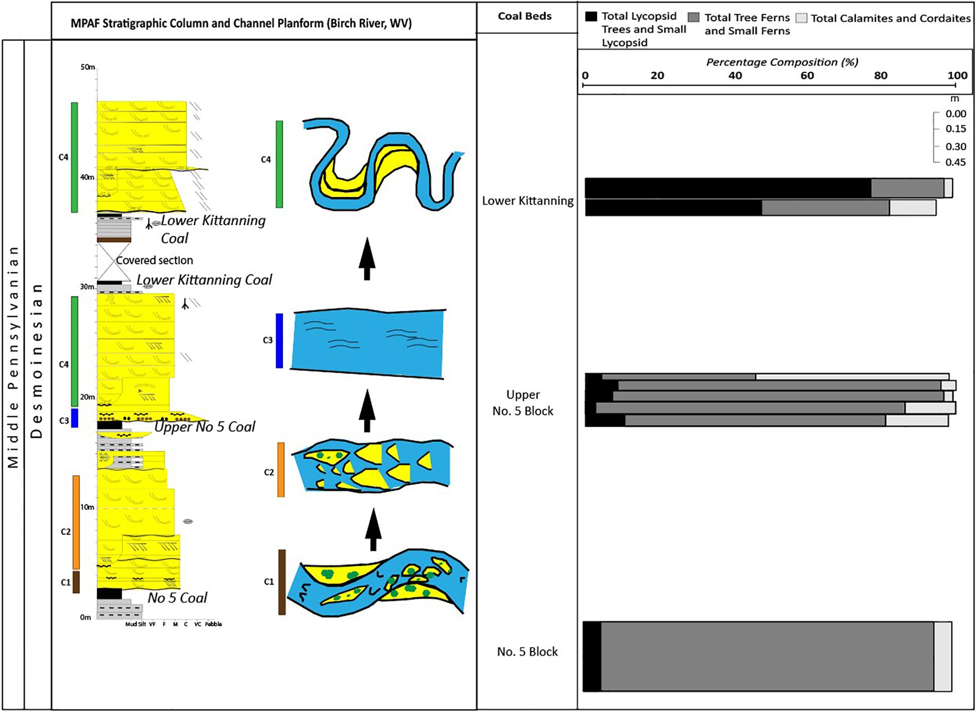
Figure 11. MPAF channel belts and distribution of numerically significant miospore taxa through time, Birch River, West Virginia. Miospore data modified from Eble (2002). CB, channel belt.

Therefore, we infer that the abundance of upper plane stage beds, low amplitude bedforms in Channel belt 3 is likely due to changes in precipitation and evapotranspiration. The fluvial depositional mechanisms of the Channel belt 3, such as paleoslope and paleohydrology, that resulted in the various bedforms of the high-velocity fluvial system may have been due to the humid to semi-arid paleoclimate change during the Pennsylvanian as modeled from Pennsylvanian paleobotany and Canadian fluvial systems (Cecil, 1990; Cecil et al., 2003; Greb et al., 2008; Allen et al., 2014). A seasonal wet–dry climate, which is common in semi-arid regions, usually results in an episodic influx of large volumes of water, which may have resulted in high-velocity floods forming the low amplitude bedforms observed in the high-velocity channel (Fielding et al., 2009; Plink-Björklund, 2015). The increase in channel depth of the sinuous channels above the LKC bed may be due to the reverse of paleoclimate to a wetter more humid climate, which is supported by the increase in lycopsid spores in the LKC beds that indicate a wet environment (Kosanke and Cecil, 1996; Eble, 2002).

Conclusion

This study used numerical modeling to highlight changes in fluvial channel geomorphology and hydrology that coincides with periods of paleoclimate change during the Middle Pennsylvanian. Measured and estimated paleochannel depth and width were used to determine changes in paleoslope and paleodischarge of the MPAF channel belts. SVR machine-assisted algorithm was effective in improving the accuracy of estimating dune heights and channel depth, from cross-set thickness. Paleochannel depth decreases during periods of increasing paleoclimate dryness; and then starts to increase during periods of increasing paleoclimate wetness. The decrease in paleochannel depth may be due to a reduction in stratigraphic base level caused by low annual precipitation, which is common in fluvial systems of seasonal wet–dry, semi-arid/semi-humid climate. Paleodischarge varies across the MPAF however, MPAF zones that experienced an increase in paleodischarge coincides with periods of paleoclimate change from ever-wet humid to seasonal semi-arid climate. Paleoslope estimates indicate low gradient physiography for the MPAF depositional environment, which agrees with previous models of ancient coal forming environments in West Virginia. Further review of possible effects of eustatic, tectonic, and paleoclimatic effect on the geometry and hydrology of fluvial systems indicated that paleoclimate was a dominant control on MPAF channel belt geomorphology and hydrology. By highlighting qualitative and quantitative characteristics of MPAF fluvial channels, this research shows a way of identifying the effects of paleoclimatic forcing on the hydrology and geomorphology of fluvial systems.

Data Availability Statement

All datasets generated for this study are included in the article/Supplementary Material.

Author Contributions

All authors listed have made a substantial, direct and intellectual contribution to the work, and approved it for publication.

Funding

Field and laboratory work for this research was made possible by funds and grants from the American Association of Petroleum Geologist (AAPG), Shumaker Fund, and West Virginia University.

Conflict of Interest

The authors declare that the research was conducted in the absence of any commercial or financial relationships that could be construed as a potential conflict of interest.

Supplementary Material

The Supplementary Material for this article can be found online at: https://www.frontiersin.org/articles/10.3389/feart.2019.00361/full#supplementary-material

References

Allen, J. P., Fielding, C. R., Gibling, M. R., and Rygel, M. C. (2014). Recognizing products of palaeoclimate fluctuation in the fluvial stratigraphic record: an example from the Pennsylvanian to Lower Permian of Cape Breton Island, Nova Scotia. Sedimentology 61, 1332–1381. doi: 10.1111/sed.12102

CrossRef Full Text | Google Scholar

Allen, J. R. (1982). Sedimentary Structures, Their Character and Physical Basis. Amsterdam: Elsevier Science & Technology.

Google Scholar

Allen, J. R. L. (1970). A quantitative model of grain size and sedimentary structures in lateral deposits. Geol. J. 7, 129–146. doi: 10.1002/gj.3350070108

CrossRef Full Text | Google Scholar

Archer, A. W., and Greb, S. F. (1995). An Amazon-scale drainage system in the early Pennsylvanian of central North America. J. Geol. 103, 611–627. doi: 10.1086/629784

CrossRef Full Text | Google Scholar

Arkle, T. Jr., Beissel, D. R., Larese, R. E., Nuhfer, E. B., Patchen, D. G., Smosna, R. A., et al. (1979). Mississippian and Pennsylvanian (carboniferous) systems in the United States: West Virginia and Maryland. U.S. Geol. Surv. Prof. Pap. 1110D, 1110.

Google Scholar

Awad, M., and Khanna, R. (2015). “Support vector regression,” in Efficient Learning Machines: Theories, Concepts, and Applications for Engineers and System Designers, eds M. Awad and R. Khanna, (Berkeley, CA: Apress), 67–80. doi: 10.1007/978-1-4302-5990-9_4

CrossRef Full Text | Google Scholar

Bao, Y., and Liu, Z. (2006). “A fast grid search method in support vector regression forecasting time series,” in Intelligent Data Engineering and Automated Learning – IDEAL 2006 Lecture Notes in Computer Science, eds E. Corchado, H. Yin, V. Botti, and C. Fyfe, (Berlin: Springer), 504–511. doi: 10.1007/11875581_61

CrossRef Full Text | Google Scholar

Bhattacharya, J. P., Copeland, P., Lawton, T. F., and Holbrook, J. (2016). Estimation of source area, river paleo-discharge, paleoslope, and sediment budgets of linked deep-time depositional systems and implications for hydrocarbon potential. Earth Sci. Rev. 153, 77–110. doi: 10.1016/j.earscirev.2015.10.013

CrossRef Full Text | Google Scholar

Blake, B. M., Cross, A. T., Eble, C., Gillespie, W. H., and Pfefferkorn, H. (2002). “Selected megafossils from the Carboniferous of the Appalachian region, eastern United States: geographic and stratigraphic distribution,” in Carboniferous and Permian of the World: Canadian Society of Petroleum Geologists Memoir 19, eds L. Hills, C. M. Henderson, and E. W. Bamber, (Calgary, AB: Canadian Society of Petroleum Geologists).

Google Scholar

Blum, M., Martin, J., Milliken, K., and Garvin, M. (2013). Paleovalley systems: insights from Quaternary analogs and experiments. Earth Sci. Rev. 116, 128–169. doi: 10.1016/j.earscirev.2012.09.003

CrossRef Full Text | Google Scholar

Blum, M. D., and Törnqvist, T. E. (2000). Fluvial responses to climate and sea-level change: a review and look forward. Sedimentology 47, 2–48. doi: 10.1046/j.1365-3091.2000.00008.x

CrossRef Full Text | Google Scholar

Bridge, J. S. (2009). Rivers and Floodplains: Forms, Processes, and Sedimentary Record. Hoboken, NJ: John Wiley & Sons.

Google Scholar

Bridge, J. S., and Mackey, S. D. (1993). “A revised alluvial stratigraphy model,” in Alluvial Sedimentation, eds M. Marzo and C. Puigdefábregas, (International Association of Sedimentologists), 317–336. doi: 10.1002/9781444303995.ch22

CrossRef Full Text | Google Scholar

Bridge, J. S., and Tye, R. S. (2000). Interpreting the dimensions of ancient fluvial channel bars, channels, and channel belts from wireline-logs and cores. Am. Assoc. Pet. Geol. Bull. 84, 1205–1228.

Google Scholar

Catuneanu, O. (2006). Principles of Sequence Stratigraphy. Amsterdam: Elsevier.

Google Scholar

Cecil, C. B. (1990). Paleoclimate controls on stratigraphic repetition of chemical and siliciclastic rocks. Geology 18, 533–536.

Google Scholar

Cecil, C. B. (2013). An overview and interpretation of autocyclic and allocyclic processes and the accumulation of strata during the Pennsylvanian–Permian transition in the central Appalachian Basin, USA. Int. J. Coal Geol. 119, 21–31. doi: 10.1016/j.coal.2013.07.012

CrossRef Full Text | Google Scholar

Cecil, C. B., Brezinski, D. K., and Dulong, F. (2004). The Paleozoic record of changes in global climate and sea level: central Appalachian basin. U.S. Geol. Surv. Circ. 1264, 77–133.

Google Scholar

Cecil, C. B., and Dulong, F. T. (2003). “Precipitation models for sediment supply in warm climates,” in Climate Controls on Stratigraphy: Society for Sedimentary Geology (SEPM), Vol. 77, eds C. B. Cecil and N. T. Edgar, (Tulsa, Ok: SEPM Society for Sedimentary Geology), 21–27. doi: 10.2110/pec.03.77.0021

CrossRef Full Text | Google Scholar

Cecil, C. B., Dulong, F. T., West, R. R., Stamm, R., Wardlaw, B., and Edgar, N. T. (2003). “Climate controls on the stratigraphy of a Middle Pennsylvanian cyclothem in North America,” in Climate Controls on Stratigraphy, eds C. B. Cecil and N. T. Edgar (Tulsa, Ok: SEPM Society for Sedimentary Geology). doi: 10.2110/pec.03.77.0151

CrossRef Full Text | Google Scholar

Cecil, C. B., Stanton, R. W., Neuzil, S. G., Dulong, F. T., Ruppert, L. F., and Pierce, B. S. (1985). Paleoclimate controls on late Paleozoic sedimentation and peat formation in the central Appalachian Basin (USA). Int. J. Coal Geol. 5, 195–230. doi: 10.1016/0166-5162(85)90014-x

CrossRef Full Text | Google Scholar

Chamberlin, E. P., and Hajek, E. A. (2015). Interpreting paleo-avulsion dynamics from multistory sand bodies. J. Sediment. Res. 85, 82–94. doi: 10.2110/jsr.2015.09

CrossRef Full Text | Google Scholar

Currie, B. S. (1997). Sequence stratigraphy of nonmarine Jurassic–Cretaceous rocks, central Cordilleran foreland-basin system. GSA Bull. 109, 1206–1222.

Google Scholar

Davidson, S. K., and Hartley, A. J. (2010). Towards a quantitative method for estimating paleohydrology from clast size and comparison with modern rivers. J. Sediment. Res. 80, 688–702. doi: 10.2110/jsr.2010.062

CrossRef Full Text | Google Scholar

Davis, J. C., and Sampson, R. J. (1986). Statistics and Data Analysis in Geology. New York, NY: Wiley.

Google Scholar

DeCelles, P. G., Langford, R. P., and Schwartz, R. K. (1983). Two new methods of paleocurrent determination from trough cross-stratification. J. Sediment. Res. 53, 629–642.

Google Scholar

DiMichele, W. A. (2013). Wetland-dryland vegetational dynamics in the Pennsylvanian ice age tropics. Int. J. Plant Sci. 175, 123–164. doi: 10.1086/675235

CrossRef Full Text | Google Scholar

DiMichele, W. A., Cecil, C. B., Montañez, I. P., and Falcon-Lang, H. J. (2010). Cyclic changes in Pennsylvanian paleoclimate and effects on floristic dynamics in tropical Pangaea. Int. J. Coal Geol. 83, 329–344. doi: 10.1016/j.coal.2010.01.007

CrossRef Full Text | Google Scholar

Donaldson, A. C., and Shumaker, R. C. (1981). “Late Paleozoic molasse of central Appalachians,” in Sedimentation and Tectonics in Alluvial Basins: Geological Association of Canada Special Paper 23, ed. A. D. Miall, (St. John’s, NL: Geological Association of Canada), 99–124.

Google Scholar

Eble, C. F. (2002). Palynology of late Middle Pennsylvanian coal beds in the Appalachian Basin. Int. J. Coal Geol. 50, 73–88. doi: 10.1016/s0166-5162(02)00114-3

CrossRef Full Text | Google Scholar

Ethridge, F. G., and Schumm, S. A. (1977). “Reconstructing paleochannel morphologic and flow characteristics: methodology, limitations, and assessment,” in Fluvial Sedimentology: Canadian Society of Petroleum Geologists Memoir, Vol. 5, ed. A. D. Miall, (Calgary, AB: Canadian Society of Petroleum Geologists), 703–722.

Google Scholar

Ettensohn, F. R. (2005). “5. The sedimentary record of foreland-basin, tectophase cycles: examples from the Appalachian Basin, USA,” in Developments in Sedimentology Cyclic Development of Sedimentary Basins, eds J. M. Mabessoone and V. H. Neumann, (Amsterdam: Elsevier), 139–172. doi: 10.1016/S0070-4571(05)80007-X

CrossRef Full Text | Google Scholar

Ettensohn, F. R. (2008). “Chapter 4 the Appalachian foreland basin in Eastern United States,” in Sedimentary Basins of the World the Sedimentary Basins of the United States and Canada, ed. A. D. Miall, (Amsterdam: Elsevier), 105–179. doi: 10.1016/s1874-5997(08)00004-x

CrossRef Full Text | Google Scholar

Falcon-Lang, H. J. (2004). Pennsylvanian tropical rain forests responded to glacial-interglacial rhythms. Geology 32, 689–692. doi: 10.1130/G20523.1

CrossRef Full Text | Google Scholar

Falcon-Lang, H. J., and Dimichele, W. A. (2010). What happened to the coal forests during Pennsylvanian glacial phases? Palaios 25, 611–617. doi: 10.2110/palo.2009.p09-162r

CrossRef Full Text | Google Scholar

Fielding, C. R., and Alexander, J. (1996). Sedimentology of the upper Burdekin River of North Queensland, Australia—an example of a tropical, variable discharge river. Terra Nova 8, 447–457. doi: 10.1111/j.1365-3121.1996.tb00770.x

CrossRef Full Text | Google Scholar

Fielding, C. R., Allen, J. P., Alexander, J., and Gibling, M. R. (2009). Facies model for fluvial systems in the seasonal tropics and subtropics. Geology 37, 623–626. doi: 10.1130/g25727a.1

CrossRef Full Text | Google Scholar

Gibling, M. R. (2006). Width and thickness of fluvial channel bodies and valley fills in the geological record: a literature compilation and classification. J. Sediment. Res. 76, 731–770. doi: 10.2110/jsr.2006.060

CrossRef Full Text | Google Scholar

Gibling, M. R., Davies, N. S., Falcon-Lang, H. J., Bashforth, A. R., DiMichele, W. A., Rygel, M. C., et al. (2014). Palaeozoic co-evolution of rivers and vegetation: a synthesis of current knowledge. Proc. Geol.Assoc. 125, 524–533.

Google Scholar

Greb, S. F., Pashin, J. C., Martino, R. L., and Eble, C. F. (2008). “Appalachian sedimentary cycles during the Pennsylvanian: changing influences of sea level, climate, and tectonics,” in Resolving the Late Paleozoic Gondwanan Ice Age in Time and Space, Vol. 441, eds C. F. Fielding, T. D. Frank, and J. L. Isbell (Tulsa, Ok: SEPM Society for Sedimentary Geology), 235–248. doi: 10.1130/2008.2441(16)

CrossRef Full Text | Google Scholar

Haq, B. U., and Schutter, S. R. (2008). A chronology of Paleozoic sea-level changes. Science 322, 64–68. doi: 10.1126/science.1161648

PubMed Abstract | CrossRef Full Text | Google Scholar

Holbrook, J., and Schumm, S. A. (1999). Geomorphic and sedimentary response of rivers to tectonic deformation: a brief review and critique of a tool for recognizing subtle epeirogenic deformation in modern and ancient settings. Tectonophysics 305, 287–306. doi: 10.1016/s0040-1951(99)00011-6

CrossRef Full Text | Google Scholar

Holbrook, J., Scott, R. W., and Oboh-Ikuenobe, F. E. (2006). Base-level buffers and buttresses: a model for upstream versus downstream control on fluvial geometry and architecture within sequences. J. Sediment. Res. 76, 162–174. doi: 10.2110/jsr.2005.10

CrossRef Full Text | Google Scholar

Holbrook, J., and Wanas, H. (2014). A fulcrum approach to assessing source-to-sink mass balance using channel paleohydrologic paramaters derivable from common fluvial data sets with an example from the Cretaceous of Egypt. J. Sediment. Res. 84, 349–372. doi: 10.2110/jsr.2014.29

CrossRef Full Text | Google Scholar

Kosanke, R. M., and Cecil, C. B. (1996). Late Pennsylvanian climate changes and palynomorph extinctions. Rev. Palaeobot. Palynol. 90, 113–140. doi: 10.1016/0034-6667(95)000275

CrossRef Full Text | Google Scholar

Leclair, S. F. (2002). Preservation of cross-strata due to the migration of subaqueous dunes: an experimental investigation. Sedimentology 49, 1157–1180. doi: 10.1046/j.1365-3091.2002.00482.x

CrossRef Full Text | Google Scholar

Leclair, S. F., and Bridge, J. S. (2001). Quantitative interpretation of sedimentary structures formed by river dunes. J. Sediment. Res. 71, 713–716. doi: 10.1306/2dc40962-0e47-11d7-8643000102c1865d

CrossRef Full Text | Google Scholar

Leeder, M. R. (1993). Tectonic Controls upon Drainage Basin Development, River Channel Migration and Alluvial Architecture: Implications for Hydrocarbon Reservoir Development and Characterization, Vol. 73. London: Geological Society, 7–22. doi: 10.1144/GSL.SP.1993.073.01.02

CrossRef Full Text | Google Scholar

Leeder, M. R. (2009). “On the interactions between turbulent flow, sediment transport and bedform mechanics in channelized flows,” in Modern and Ancient Fluvial Systems, eds J. D. Collinson and J. Lewin, (London: Wiley-Blackwell), 3–18. doi: 10.1002/9781444303773.ch1

CrossRef Full Text | Google Scholar

Lin, W., and Bhattacharya, J. P. (2017). Estimation of Source-to-sink mass balance by a fulcrum approach using channel paleohydrologic parameters of the Cretaceous Dunvegan Formation, Canada. J. Sediment. Res. 87, 97–116. doi: 10.2110/jsr.2017.1

CrossRef Full Text | Google Scholar

Miall, A. (2014). Fluvial Depositional Systems. Cham: Springer International Publishing. doi: 10.1007/978-3-319-006666

CrossRef Full Text | Google Scholar

Miall, A. D. (1996). The Geology of Fluvial Deposits. Berlin: Springer.

Google Scholar

Montañez, I. P., McElwain, J. C., Poulsen, C. J., White, J. D., DiMichele, W. A., Wilson, J. P., et al. (2016). Climate, pCO2 and terrestrial carbon cycle linkages during late Palaeozoic glacial–interglacial cycles. Nat. Geosci. 9, 824–828. doi: 10.1038/ngeo2822

CrossRef Full Text | Google Scholar

Pedregosa, F., Varoquaux, G., Gramfort, A., Michel, V., Thirion, B., Grisel, O., et al. (2011). Scikit-learn: machine learning in Python. J. Mach. Learn. Res. 12, 2825–2830.

Google Scholar

Peppers, R. A. (1996). Palynological Correlation of Major Pennsylvanian (Middle and Upper Carboniferous) Chronostratigraphic Boundaries in the Illinois and other Coal Basins. Boulder, CO: Geological Society of America.

Google Scholar

Plink-Björklund, P. (2015). Morphodynamics of rivers strongly affected by monsoon precipitation: review of depositional style and forcing factors. Sediment. Geol. 323, 110–147. doi: 10.1016/j.sedgeo.2015.04.004

CrossRef Full Text | Google Scholar

Python (2019). Python Software Foundation. Python.Org. Available at: https://www.python.org/ (accessed June 28, 2019).

Google Scholar

Rubin, D. M., and McCulloch, D. S. (1980). Single and superimposed bedforms: a synthesis of San Francisco Bay and flume observations. Sediment. Geol. 26, 207–231. doi: 10.1016/0037-0738(80)90012-3

CrossRef Full Text | Google Scholar

Sak, P. B., McQuarrie, N., Oliver, B. P., Lavdovsky, N., and Jackson, M. S. (2012). Unraveling the central Appalachian fold-thrust belt, Pennsylvania: the power of sequentially restored balanced cross sections for a blind fold-thrust belt. Geosphere 8, 685–702.

Google Scholar

Schumm, S. A. (1968). River Adjustment to Altered Hydrologic Regimen-Murrumbidgee River and Paleochannels, Australia. Washington, DC: US Government Printing Office.

Google Scholar

Schumm, S. A. (1981). “Evolution and response of the fluvial system, sedimentologic implications,” in Recent and Ancient Nonmarine Depositional Environments, eds P. G. Ethridge and K. M. Flores, (Tulsa, OK: Society for Sedimentary Geology).

Google Scholar

Schumm, S. A. (1988). Variability of the fluvial system in space and time. Scales Glob. Change 35, 225–250.

Google Scholar

Shanley, K. W., and McCabe, P. J. (1994). Perspectives on the sequence stratigraphy of continental strata. Am. Assoc. Pet. Geol. Bull. 78, 544–568.

Google Scholar

Stubbs, D. G. (2018). A Sequence Stratigraphic Analysis of the Allegheny Group (Middle Pennsylvanian), Southeast Ohio. Masters thesis, Ohio University, Athens, OH.

Google Scholar

Tabor, N. J., and Montanez, I. P. (2002). Shifts in late Paleozoic atmospheric circulation over western equatorial Pangea: insights from pedogenic mineral δ18O compositions. Geology 30, 1127–1130.

Google Scholar

Tabor, N. J., and Poulsen, C. J. (2008). Palaeoclimate across the Late Pennsylvanian–Early Permian tropical palaeolatitudes: a review of climate indicators, their distribution, and relation to palaeophysiographic climate factors. Palaeogeogr. Palaeoclimatol. Palaeoecol. 268, 293–310. doi: 10.1016/j.palaeo.2008.03.052

CrossRef Full Text | Google Scholar

Zhang, Y., Kimberg, D. Y., Coslett, H. B., Schwartz, M. F., and Wang, Z. (2014). “Support vector regression based multivariate lesion-symptom mapping,” in Proceedings of the 36th Annual International Conference of the IEEE Engineering in Medicine and Biology Society (Chicago, IL: IEEE), 5599–5602.

Google Scholar