Petrophysical Joint Inversion Applied to Alpine Permafrost Field Sites to Image Subsurface Ice, Water, Air, and Rock Contents

1. Introduction

Permanently frozen soils are a sensitive climate indicator and the ongoing permafrost degradation is likely to accelerate further in the future (IPCC, 2019), as high latitude and mountain chains are regions, which are especially sensitive to climate change induced temperature increase (e.g., Pepin et al., 2015). Permafrost is an invisible thermal phenomenon (defined as ground at or below 0°C during at least 2 years, Harris et al., 1988). Ground temperature increase near the ice melting point leads to permafrost thaw and may affect mountain slope stability (Ravanel et al., 2017). Quantification of the volumetric ground ice content is therefore an important means to understand the current state of alpine permafrost as well as to monitor its future evolution. Ground ice content can typically vary from 0 to 100%, depending on the permafrost landform, from ice-poor bedrock to ice-rich talus slope or rock glaciers (e.g., Kenner et al., 2019).

Ice content is a key factor in permafrost studies (e.g., Scherler et al., 2013) and is generally unknown as it is especially difficult to assess quantitatively and even more challenging to monitor. Exceptions are studies analysing ice cores of e.g., rock glaciers with the aim to directly measure the ice content in one dimension (Haeberli et al., 1988; Monnier and Kinnard, 2013; Krainer et al., 2015). Borehole-derived ground ice analyses from multiple boreholes and extrapolation over a large area was undertaken by Wang et al. (2018). Nuclear well logging methods were also used to quantify the porosity and the ice content in one dimension (Barsch et al., 1979; Scapozza et al., 2015).

Boreholes are however costly and logistically difficult in high mountain terrain. In many permafrost studies, the detection of ground ice is therefore undertaken through indirect and non-destructive geophysical methods, such as electrical resistivity tomography (ERT), ground penetrating radar, refraction seismic tomography (RST), or gravimetry (e.g., Hauck and Kneisel, 2008). ERT is the most commonly used method due to the high sensitivity of electrical resistivity to the presence or absence of liquid water and the relatively short time needed for data acquisition and processing (e.g., Kneisel et al., 2008). Also repeated RST measurements can yield an estimation of ground ice variation (e.g., Hilbich, 2010; Draebing, 2016). Ground penetrating radar surveys are often conducted to characterize the internal composition and structure of e.g., rock glaciers (e.g., Degenhardt, 2003; Hausmann et al., 2007; Maurer and Hauck, 2007; Monnier and Kinnard, 2013; Merz et al., 2016). Gravimetric measurements were performed to delineate zones characterized by different ice content within rock glaciers (e.g., Vonder Mühll and Klingelé, 1994; Hausmann et al., 2007). Hausmann et al. (2007) quantified the total ice content of a rock glacier by carrying out gravimetrical, ground penetrating radar, and seismic measurements to estimate the ice content assuming an a priori air content and the absence of liquid water content. New approaches include the possible estimation of ground ice variation through subsidence measurements using reflected GNSS signals (Liu and Larson, 2018) or through spaceborne gravity measurements (e.g., Vey et al., 2012). Since information from one method is often ambiguous, many cryogeophysical studies use a combination of different geophysical methods (e.g., Hausmann et al., 2007; Kneisel et al., 2008; Doetsch et al., 2012; Buchli et al., 2013; Parsekian et al., 2015; Briggs et al., 2016; Merz et al., 2016; Pellet et al., 2016; Emmert and Kneisel, 2017; Léger et al., 2017; Mewes et al., 2017).

Seismic and electrical methods have complementary sensitivities and are often combined in different ways (e.g., Zhang and Morgan, 1997; Gallardo and Meju, 2004; Garofalo et al., 2015; Ronczka et al., 2017). Carcione et al. (2007) reviewed the cross-property relations between electrical conductivity and seismic velocity. They choose the porosity as the key property permitting to establish relationships between these two physical parameters. The so-called four-phase model (4PM) developed by Hauck et al. (2011) estimates ice, water and air contents from simple petrophysical relations involving electrical resistivities and seismic velocities. The 4PM was applied successfully in several recent permafrost studies (Pellet et al., 2016; Hauck et al., 2017; Mewes et al., 2017). However, the approach requires to prescribe the porosity and is based on individual seismic and electric inversions with the danger of introducing physical inconsistencies in the final results.

To fully exploit two independent geophysical datasets and to improve the reliability of the individual results, several possibilities exist: (i) joint interpretation of two datasets (as in the above cited studies), (ii) joint inversion, where datasets exploit complementary sensitivities (e.g., structural joint inversion), and (iii) joint inversion of one common parameter (e.g., water saturation or porosity) from two separate datasets (petrophysical joint inversion). In the present paper we focus on the latter approach, i.e., the inversion of several common parameters from two independent geophysical methods.

Inverse theory has been extensively used for decades in applied natural sciences to analyse data (Menke, 1989), whereas the concept of joint inversion itself was introduced in 1975 by Vozoff and Jupp. Zhang and Morgan (1997) can be counted among the first to develop joint inversion strategies for physically uncorrelated datasets (e.g., seismic velocities and electrical resistivities). Many modern joint inversion algorithms have been developed to improve the inversion results, reduce the uncertainties and incorporate a priori knowledge (e.g., Gallardo and Meju, 2004; Doetsch et al., 2010; Karaoulis et al., 2013; Garofalo et al., 2015; Linde and Doetsch, 2016; Hellman et al., 2017).

Two main approaches of joint inversion are co-existing in the literature: structural and petrophysical joint inversion (e.g., Gallardo and Meju, 2004). Structural joint inversion is based on the assumption that geophysical subsurface images from unrelated physical properties are associated to the same geological structure (e.g., Garofalo et al., 2015). The similarity between both images can be expressed by the so-called cross-gradient function. In petrophysical joint inversions (PJI), common material properties (often porosity or water content) are used as the link between electrical resistivity and P-wave velocity for example (e.g., Carcione et al., 2007; Garofalo, 2014; Rücker et al., 2017).

To improve the characterization of the composition of frozen ground, Wagner et al. (2019) developed a PJI framework to quantify water, ice, and air contents from geophysical datasets based on the 4PM approach (Hauck et al., 2011). The approach was successfully validated on synthetic datasets and a proof-of-concept field application (Schilthorn field site). Theoretically, the major advantages of this approach in comparison with the original 4PM are: (i) its physical consistency between the electrical and seismic datasets and the obtained subsurface composition, (ii) the possibility to estimate the rock content, which is inverted together with the three pore constituents, as part of the output model parameter vector (the rock content has to be prescribed in the original 4PM), and (iii) the possibility to incorporate non-geophysical information on the petrophysical target parameters in the inversion.

The objectives of this contribution are to (i) apply and extend the algorithm developed by Wagner et al. (2019) by testing different petrophysical relations and apply them to several field sites, which represent a high diversity of mountain permafrost landforms, from ice-poor to ice-rich grounds, (ii) analyse the influence of the regularization parameters, and (iii) validate the results with borehole data (temperature and direct or indirect measurements of ice content data). Different equations linking the electrical resistivity to water content (taking into account the electrolytic conduction, the surface conduction, or both) are explored. Furthermore we analyse whether the PJI in general or the specific petrophysical equations in detail are more applicable for certain field site characteristics. Finally, an assessment of the added value of a PJI approach compared to standard geophysical interpretations is proposed and remaining challenges are discussed.

2. Method

2.1. Origin of the Approach

The original 4PM consists of a system of simple petrophysical equations (Archie's second law and Timur's time-average equation) with input data consisting of porosity, P-wave velocities derived from inverted travel times, and the inverted electrical resistivities. Output data are subsurface ice, water and air content (Hauck et al., 2011). The 4PM has undergone a constant improvement since its development (Python, 2015; Pellet et al., 2016; Hauck et al., 2017), but the porosity always needs to be prescribed (cf. Figure 1A), although it is mostly unknown.

FIGURE 1

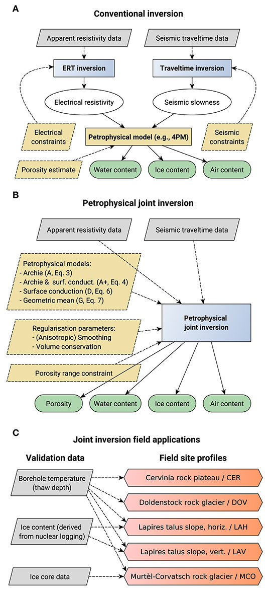
Figure 1. Schematic on the estimation of water, ice, and air from electrical resistivity and refraction seismic data (modified after Wagner et al., 2019). (A) Conventional inversion of both datasets with subsequent petrophysical transformation. (B) Petrophysical joint inversion honoring both datasets and petrophysical relations during parameter estimation. (C) Field applications and validation data of this paper.

The basic constraint of the model is the assumption that the subsurface is composed of the volumetric fractions of four phases: the rock matrix f_r, water f_w, ice f_i, and air f_a:

$\begin{array}{ll}{f}_{\text{r}}+f_{\text{w}}+f_{\text{i}}+f_{\text{a}}=1& (1)\end{array}$

The ice fraction is hereby an additional model parameter compared to most applied hydrogeophysical studies (e.g., Linde and Doetsch, 2016), whereas the air fraction is absent in the system of equations under saturated conditions (e.g., Rücker et al., 2017). In these cases, the number of model parameters in the system reduces to three (air or ice content assumed to be zero), contrary to most permafrost field cases, where all four phases can have strictly positive values. However, by using uncoupled electrical and seismic data (individual inversions, cf. Figure 1A), their use in separate petrophysical equations may lead to non-physical results, i.e., volumetric contents below zero or larger than one, which, as a sum, may still satisfy Equation (1).

These shortcomings led to the recent development of a joint inversion code to fully use the complementarity of independent geophysical data (Wagner et al., 2019). Figures 1A,B highlight the conceptual differences of both inversion approaches. In the original 4PM, both the apparent electrical resistivities and the refraction seismic travel times are inverted individually, and assuming a porosity distribution, the inverted resistivities and seismic velocities are then used in a system of petrophysical equations to retrieve the water, ice and air contents (Figure 1A). In the PJI (details are given in section 2.3), the apparent resistivities and travel times are used to directly and jointly invert for rock, ice, water, and air contents (Figure 1B). Petrophysical equations and additional porosity constraints as well as regularization parameters appear in the joint inversion core equations (yellow boxes in Figure 1B). These yellow boxes in Figure 1B and the field applications and validation (Figure 1C) constitute the scope of this paper.

2.2. Petrophysical Relations

Both P-wave velocity and electrical resistivity are sensitive to ice-to-water phase changes (Scott et al., 1990). However, no analytical relationship exists between resistivity and P-wave velocity (Gallardo and Meju, 2003). To develop a PJI scheme for geoelectric and seismic measurement data, the corresponding petrophysical relationships have to be combined.

Numerous petrophysical relationships for seismic velocity and electrical resistivity are available in the literature, including cross-property relations representing a given type of rock based on experimental data (e.g., Carcione et al., 2007; Glover, 2010). For the seismic data, we use the time-average equation (Equation 2) to predict the bulk velocity v from the constituent fractions and their individual velocities, which is an extension of the time-average approach by Timur (1968) to account for all four phases present in permafrost (cf. Hauck et al., 2011):

$\begin{array}{ll}\frac{1}{v}=\frac{f_{\text{r}}}{v_{\text{r}}}+\frac{f_{\text{w}}}{v_{\text{w}}}+\frac{f_{\text{i}}}{v_{\text{i}}}+\frac{f_{\text{a}}}{v_{\text{a}}}& (2)\end{array}$

The four phase velocities are named similarly to the volumetric fractions: v_r, v_w, v_i, v_a. Their values are considered constant and equal to values found in the literature (e.g., Hauck et al., 2011).

Archie's law (Archie, 1942) is used in the original 4PM and also for the PJI study by Wagner et al. (2019), although other relationships were tested within the conventional 4PM (e.g., unpublished Master thesis, Python, 2015). The electrical resistivity ρ (or conductivity σ) combines the contribution of three conduction mechanisms: particle conduction, surface conduction, and electrolytic conduction (e.g., Klein and Santamarina, 2003). According to Duvillard et al. (2018), the surface conduction is often (and incorrectly) neglected in geophysical studies using the original Archie's law. In the following, we therefore compare and test four different relations linking ρ with the respective ground properties.

2.2.1. Archie's Law (Model A)

Archie's second law is one of the oldest and most often used relations linking the bulk resistivity ρ with the pore water content (Archie, 1942, Equation 3) and is generally recognized as valid when electrolytic conduction dominates, an assumption, that is, however, not always justified.

$\begin{array}{ll}\rho ={\rho }_{\text{w}}{(1-f_{\text{r}})}^{-m}{\left(\frac{f_{\text{w}}}{1-f_{\text{r}}}\right)}^{-n}& (3)\end{array}$

ρ_w, m and n denote hereby the pore water resistivity, the cementation exponent and the saturation exponent (Archie, 1942), respectively. Without detailed site-specific knowledge, the empirical parameters m and n are assumed constant over space.

2.2.2. Archie's Law With Surface Conduction Factor (Model A+)

Several modified versions of Archie's law were developed to account for contributions from additional conduction processes, such as surface conduction (e.g., Sen et al., 1988; Glover, 2010). Equation (4) is a modified form of Waxman and Smits (1968) and Sen et al. (1988) accounting for unsaturated conditions (see also e.g., Friedel et al., 2006; Revil et al., 2014). We follow the notation of Python (2015), who introduced the factor ε (in S/m, Equation 4) to account for surface conduction in addition to electrolytic conduction. Equation (4) is named A+ (i.e., Archie's law with surface conduction factor) in the following.

$\begin{array}{ll}\rho =\frac{{\rho }_{\text{w}}}{1+\epsilon {\rho }_{\text{w}}}{(1-f_{\text{r}})}^{-m}{\left(\frac{f_{\text{w}}}{1-f_{\text{r}}}\right)}^{-n}& (4)\end{array}$

2.2.3. Surface Conduction Model (Model D)

At very low pore water salinity in the often dry and ion-poor substrates in mountain permafrost, surface conduction may also play the dominant role and electrolytic conduction can be neglected. According to Duvillard et al. (2018), in these cases, the bulk resistivity can be derived as follows:

$\begin{array}{ll}\rho =\frac{1}{\sigma }=\frac{1}{{\sigma }_{\text{w}}{(f_{\text{w}})}^2+b{f}_{\text{w}}}& (5)\end{array}$

with pore water conductivity σ_w = 1/ρ_w and b = ρ_gB CEC. ρ_g denotes the grain density (in kg/m³), B denotes the apparent mobility of the counterions for surface conduction (in m²/V/s), and CEC is the cation exchange capacity (in C/kg). CEC can vary by several orders of magnitude for different types of material (e.g., Coperey et al., 2019). In the case of low pore water salinity (σ_w ≃ 0), the resistivity can be approximated by the expression of surface conduction only (Duvillard et al., 2018), named model D in the following:

$\begin{array}{ll}\rho =\frac{1}{b{f}_{\text{w}}}& (6)\end{array}$

As measurements or estimations of the variables B and CEC are rare and difficult to obtain for real-world cases in high mountain environments, and as the constituents of the parameter b likely vary significantly in space and especially with depth, where measurements are difficult to perform (or numerous samples expensive to retrieve), we choose to apply Equation (6) with the factor b spanning over a large range of values including the values measured by Duvillard et al. (2018) to test this approach within our joint inversion framework. The factor b was found to be on the order of magnitude of 10⁻⁷ S/m by Duvillard et al. (2018).

2.2.4. Resistivity Geometric Mean Model (Model G)

Finally, the geometric mean model assumes random distributions of the four phases, i.e., arbitrary shaped and orientated volumes of the four phases (Glover, 2010):

$\begin{array}{ll}\rho ={\rho }_{\text{r}}^{f_{\text{r}}}·{\rho }_{\text{i}}^{f_{\text{i}}}·{\rho }_{\text{w}}^{f_{\text{w}}}·{\rho }_{\text{a}}^{f_{\text{a}}}& (7)\end{array}$

with ρ_r, ρ_a, and ρ_i, the resistivity of the rock, air and ice, respectively. Equation (7) has the advantage to include the fractions of the four phases (in contrast to the three other models A, A+, and D, where both the ice and air contents do not appear explicitly and are therefore not constrained by these equations). The geometric mean model (G) has however the disadvantage to add more unknowns in the system of equations, such as the rock matrix resistivity (which can also vary in space). Figures S1, S2 highlight the differences in the solution space between the 4PM using Archie's law (model A) and the resistivity geometric mean model (model G).

2.3. Petrophysical Joint Inversion Scheme

Wagner et al. (2019) developed a PJI scheme for four phases leveraging on the forward modeling capabilities available in pyGIMLi (Rücker et al., 2017). They implemented the modified Timur's equation and Archie's law (Equations 2 and 3, as in Hauck et al., 2011) to validate the approach for synthetic datasets and a proof-of-concept field application at the Schilthorn monitoring site. The pyGIMLi-based code is conceived flexible to apply additional constraints or to apply other petrophysical relationships, which facilitates comparison studies as presented in this work.

In the following, we follow the notation of Wagner et al. (2019). The input data vector d contains the travel times t and the logarithm of apparent resistivities ρ_a to ensure positivity (Equation 8), whereas the output parameter vector p contains the volumetric fractions of rock, water, ice, and air (Equation 9):

$\begin{array}{ll}d={\left[t,log({\rho }_{\text{a}})\right]}^T& (8)\end{array}$

with ^T denoting the transpose matrix.

$\begin{array}{ll}p={\left[f_{\text{w}},f_{\text{i}},f_{\text{a}},f_{\text{r}}\right]}^T& (9)\end{array}$

The inversion itself consists of minimizing the following objective function (Wagner et al., 2019):

$\begin{array}{ll}\parallel W_{\text{d}}(d-{F}(m)){\parallel }_2^2+{\alpha }^2\parallel W_{\text{m}}m{\parallel }_2^2+{\beta }^2\parallel W_{\text{p}}^{\text{sum}}p-1{\parallel }_2^2\to min.& (10)\end{array}$

The first term of Equation (10) corresponds to the misfit between the data vector d and the model response ${F}(m)$ incorporating the data errors in the data weighting matrix W_d. As we do not have an accurate estimate of data errors, W_d includes two data error values, err_ρa and err_tt, applied for all apparent resistivity data and all travel time data, respectively, which correspond to the root mean square errors (RMS) found by the respective individual inversions.

The second term corresponds to a smoothness regularization applied to the model vector m, where α denotes the smoothness regularization parameter and where the model smoothing matrix W_m serves to enhance smoothness in the distribution of each constituent of the parameter vector.

The third term represents a supplementary regularization term to fulfill the volume conservation constraint in Equation (1). β denotes hereby the volumetric conservation regularization parameter. $W_{\mathrm{\text{p}}}^{\mathrm{\text{sum}}}$ is a matrix of four adjacent identity matrices acting on the parameter vector p to favor solutions for which the sum of the four volumetric fractions approaches unity. See Wagner et al. (2019) for more details on the PJI scheme.

Constraint setting is flexible for each model parameter (within a fourth optional term in the objective function, Wagner et al., 2019). At first, the porosity ϕ (i.e., 1 − f_r) is constrained within a conservative physically plausible range (between ϕ_min and ϕ_max). The three pore fractions are constrained physically between zero and porosity. By this and the penalization of solutions, which do not conserve the volume (Equation 1) in the objective function, non-physical solutions of the inverse problem are avoided. If a priori knowledge is available, the volumetric fractions can be further constrained, i.e., their possible range can be reduced.

3. Field Sites and Datasets

3.1. Geophysical Datasets

The input data of the joint inversion problem consist of compressional wave travel times and apparent electrical resistivities. Apparent resistivity data were acquired through a Geotom instrument (Geolog, Germany) or a Syscal resistivity meter (Iris Instruments, France) and were filtered following the procedure described in Mollaret et al. (2019). Seismograms were recorded through a Geode system (Geometrics, USA). First breaks were picked manually within the software REFLEXW (Sandmeier, 2019).

ERT and RST profiles are collocated for each site described in the following. Survey geometry set-up is given in Table 1 indicating sensor number and interval as well as ERT acquisition scheme and the number of seismic shoot points. For illustration, we obtained individually inverted tomograms of each profile presented in Figure 2 using the open-source library pyGIMLi (Rücker et al., 2017). Their dates of measurements and the resulting individual RMS errors are indicated in Figure 2. Resolution capacity and data quality differ for each site and method (cf. RMS error and the geometrical set-up indicated in Figure 2 and in Table 1, respectively).

TABLE 1

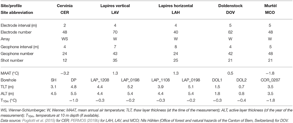
Table 1. Summary of ERT and RST profile set-ups and borehole characteristics.

FIGURE 2

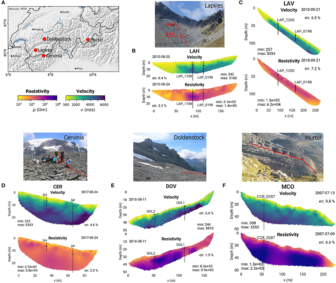
Figure 2. (A) Field site location map, field site photographs with red lines indicating the geophysical profile position, and electrical resistivity and refraction seismic tomograms (individual inversions) for (B) LAH, (C) LAV, (D) CER, (E) DOV, and (F) MCO. In the tomograms, the vertical axis is exaggerated by 50% for a better readability. The individual RMS error of each tomogram is indicated nearby, as well as the date of measurements and the minimum and maximum values of the tomograms. Black lines indicate the borehole and thaw layer positions.

3.2. Field Sites

For the evaluation of the applicability of the PJI for a wide range of permafrost landforms and materials, we choose several field sites from our monitoring network including bedrock, talus slope, and rock glacier sites and from ice-poor to ice-rich conditions. The chosen sites are located in four different regions of the northwestern Alps (Figure 2A).

Borehole temperature information and ice content were used as validation data (Figure 1C). Table 1 summarizes site and borehole information of the study sites. In the following, each of the four sites (including five profiles) is shortly described including a geophysical interpretation from the independent inversions (see Figure 2). In addition to these five profiles, the results of Wagner et al. (2019) of the proof-of-concept Schilthorn site are reproduced in section 5.2 for comparison purposes. The Schilthorn field site, located in the Bernese Alps, Switzerland, has been extensively investigated (e.g., Hilbich et al., 2008, 2011; Pellet et al., 2016). Wagner et al. (2019) offer a detailed description of the site and data used within the joint inversion (which is not repeated here).

3.2.1. Cervinia Rock Plateau

The Cervinia field site (CER) is located on the high-altitude plateau (3,100 m a.s.l.) of Cime Bianche in the Aosta valley, Italy (45° 55′09″N, 7° 41′34″E).

Sporadic bedrock outcrops are visible in the highly weathered surface layer of fine-grained to coarse-grained debris of mica schists (up to a couple of meters thick).

Ground temperatures are monitored in two boreholes by the Environmental Protection Agency of Aosta Valley (ARPA, Pogliotti et al., 2015).

Annual geophysical measurements of the same profile are performed since 2013 (Pogliotti et al., 2015; Pellet et al., 2016; Mollaret et al., 2019). In the tomogram in Figure 2D, the lowest velocities (corresponding to a high air content) occurring in the near-surface are interpreted to be a porous debris layer. The highest surface velocities around borehole DP correspond to weathered bedrock outcrops. The thaw layer is however hardly discernible from ERT and RST.

3.2.2. Lapires Talus Slope

The Lapires site is an alpine talus slope located at 2,500 m a.s.l. in the Valais Alps, Western Switzerland (6° 06′22″N, 7° 17′04″E). Its lithology mainly consists of gneiss. Excavation during the construction of a chairlift pylon proved the presence of ground ice in the talus slope (Delaloye and Lambiel, 2005). Staub et al. (2015) used ground surface temperature data to create a local permafrost distribution map, which highlights the occurrence of large patches of permafrost, but not covering the whole talus slope. The talus slope is characterized by the occurrence of internal convective air circulation, causing a net cooling especially in the lower part of the slope (Delaloye and Lambiel, 2005). Four boreholes were drilled in the Lapires talus slope, one in 1998 and three in 2008 (including one without permafrost) (PERMOS, 2013, 2019b).

Geophysical measurements were performed along two orthogonal profiles: the Lapires horizontal profile (LAH, Hilbich, 2010; Mollaret et al., 2019; PERMOS, 2019a) and the Lapires vertical profile (LAV, PERMOS, 2013; Scapozza, 2013). Hilbich (2010) investigated and jointly interpreted seasonal changes in electrical resistivities and seismic travel times at LAH.

Scapozza et al. (2015) carried out radioactivity logs at two boreholes in 2010 to quantitatively estimate the ice content and the apparent porosity from gamma-gamma and neutron-neutron logs, respectively. The two independent logging methods are consistent to each other, which confirms the robustness of the approach. Ice content estimations by nuclear logging highlight partially ice saturated to supersaturated conditions (Scapozza et al., 2015). The two boreholes (LAP_1108 and LAP_1208) are each located along one of the two profiles (see Figures 2B,C). The considered ERT and RST measurements were conducted shortly before the well logging (about a month earlier at LAH/LAP_1108).

Low velocities occur within the uppermost 4–5 m thick layer, as well as on the left of both LAH and LAV profiles (Figures 2B,C). They indicate the absence of ice and a high porosity (filled by air, cf. Scapozza, 2013). High resistivities in combination with intermediate velocities (3,000–4,000 m/s) are interpreted to correspond to the highest ice contents (see Figures 2B,C). Maximum velocities do mostly not exceed 4000 m/s and indicate that no bedrock was encountered down to ~ 20 m depth (except for the lowermost part of LAV).

3.2.3. Doldenstock Rock Glacier

The Doldenstock field site is located at 2,550 m a.s.l. in the Bernese Alps, Switzerland (46° 28′42″N, 7° 42′37″E). Typical creeping structures indicate the presence of a rock glacier. The lithology is dominated by limestones and marls (Federal Office of Topography Swisstopo, 2019). Outcropping bedrock was observed further up-slope, but not along the geophysical profiles.

From the two orthogonal geophysical profiles carried out on the rock glacier in summers 2015 and 2016 (Hilbich et al., 2019), the vertical profile (DOV, see Figure 2E), crosses the main part of the rock glacier and continues over the rooting part zone in its upper part. Two boreholes (DOL1 and DOL2) were drilled along this vertical profile in 2016. Bedrock was encountered at 6 and 16 m depth, below a 4.5 and 15 m thick layer of massive ice, respectively (Hilbich et al., 2019).

The rock glacier is characterized by very high resistivities (>10⁵Ωm) occurring at depth in the center of the profile (between the boreholes), which coincide with moderate velocities (3,000–4,000 m/s), suggesting ice-rich conditions. On the contrary, high velocities (6,000–7,000 m/s) with medium resistivities (10⁴ − 10⁵Ωm) indicate the bedrock in the upper part of the profile (see Figure 2E).

3.2.4. Murtèl-Corvatsch Rock Glacier

The Murtél-Corvatsch field site (MCO) is located at 2,670 m a.s.l. in the Engadine Valley, Eastern Swiss Alps, Switzerland (46° 25′44″N, 9° 49′18″E). This rock glacier has been extensively studied since 1987, when a deep borehole was drilled (Haeberli et al., 1988; Hoelzle et al., 2002). Drill core analysis proved the presence of massive ice with up to 80 to 100 Vol. % ice content. Since then, numerous geophysical measurements were carried out (Vonder Mühll and Klingelé, 1994; Maurer and Hauck, 2007; Schneider et al., 2013). Hilbich et al. (2009) assessed the feasibility of ERT monitoring techniques on coarse-debris ground, such as Murtèl rock glacier.

Since 2006, annual ERT monitoring measurements are conducted (Hilbich et al., 2009; Mollaret et al., 2019), and a seismic profile was measured in 2007 along the same line. Extremely high resistivity values can indicate either high ice or air content. In the MCO tomogram in Figure 2F, resistivities up to ~2.10⁶Ωm for depths >5 m correlate with moderate velocity values (about 3,500 m/s), and evidence a high ice content, which is confirmed by ice core data (Haeberli et al., 1988) as well as ground penetrating radar surveys (Maurer and Hauck, 2007). Due to the coarse-blocky material, even the unfrozen active layer exhibits relatively large resistivities of ~ 10⁴ − 10⁵Ωm, which is due to the large air-filled voids.

4. Results

4.1. Porosity Constraint Influence

One of the main advantages of the joint inversion code developed by Wagner et al. (2019) in comparison with the 4PM developed by Hauck et al. (2011) is the estimation of the rock content, which is inverted together with the three pore constituents as part of the output model parameter vector (cf. Equation 9). Consequently, the system of equations has more model parameters than data. Hence, the more a priori information we implement, the more constrained will be the system. In most field cases, a priori knowledge of the porosity distribution can be incorporated, such as a reduction of the possible porosity range, e.g., porosity is usually lower than 0.7 where bedrock outcrops are visible.

To illustrate this dependency on the porosity constraint, the petrophysical joint inversion has been run for the Cervinia rock plateau using the extended Timur's equation (Equation 2) and Archie's second law (model A, Equation 3), with the parameters specified in Table 2 and for three different porosity ranges. Figure 3 shows the resulting four-phase distribution with one subplot for each volumetric fraction as well as their sum in the bottom row. Figure 3A represents a case without any a priori information (the porosity being constrained between ϕ_min = 0 and ϕ_max = 1 and the initial porosity ϕ_start being 0.5, i.e., the median value of all physically possible values), whereas Figures 3B,C show two cases of constrained porosity ranges.

TABLE 2

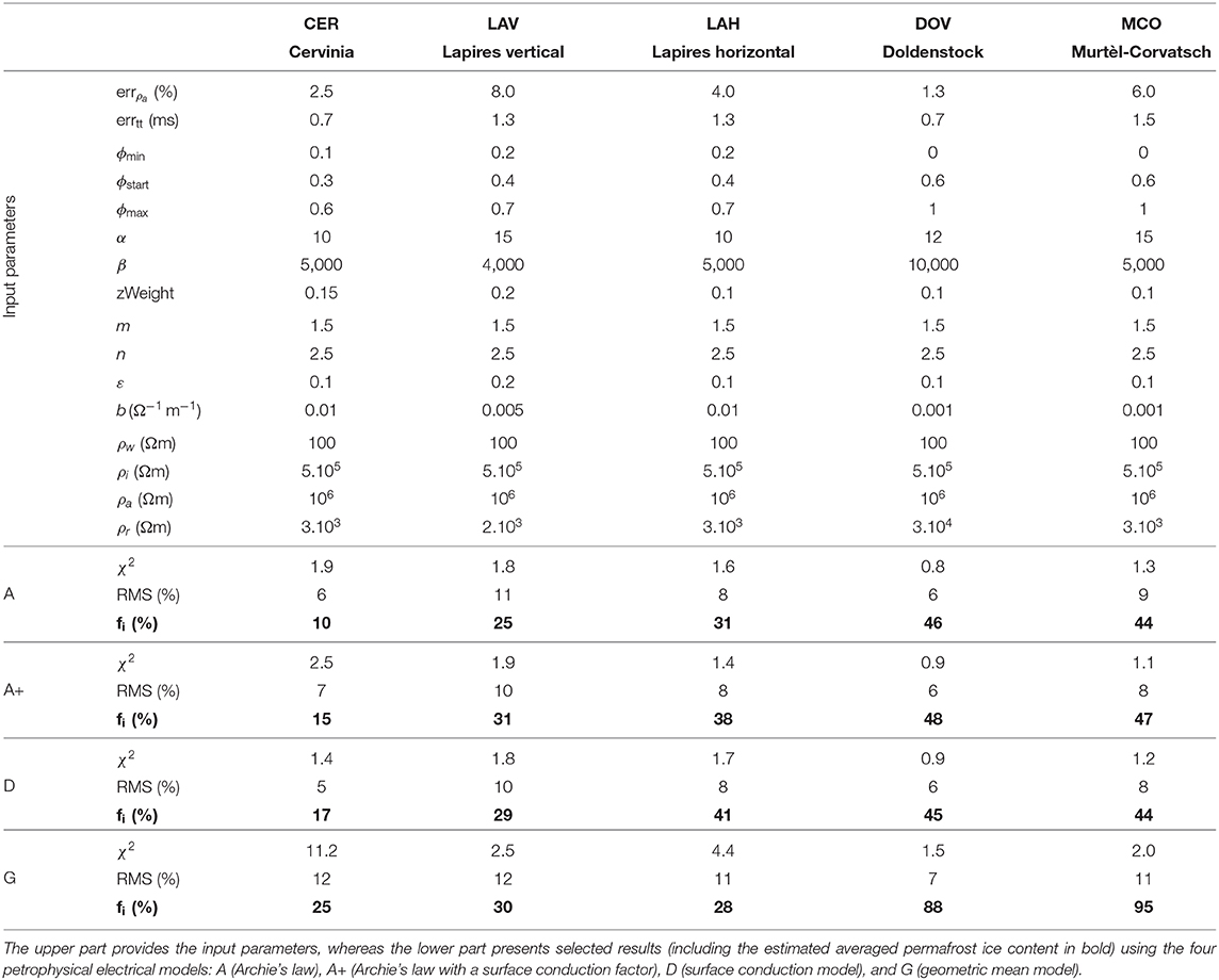
Table 2. Summary of selected parameters for each profile.

FIGURE 3

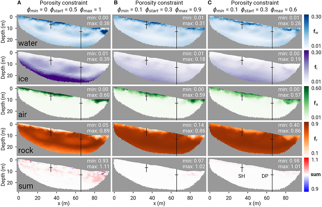
Figure 3. Joint inversion results for the Cervinia profile with volumetric fractions of water f_w, ice f_i, air f_a, rock matrix f_r, and their sum using Archie's law, shown for three different porosity constraints: (A) without a priori knowledge, (B) with a homogeneous start porosity model ϕ_start = 0.3 and excluding extreme values (0.1 < ϕ < 0.9), and (C) limiting in addition maximum porosity ϕ_max = 0.6. Boreholes and associated thaw depths are marked by black lines. Minimum and maximum phase fractions are indicated for each tomogram.

The water and air contents generally decrease with depth, whereas the ice and rock contents generally increase with depth. The comparison of all three cases shows that the porosity constraint has little influence on water and air contents. The air content reaches values up to 60% at the surface (porous debris layer) and approaches 0% from 5 m depth downwards and in the bedrock. Up to 30% water content is found near the surface, whereas values around 5–10% are characteristic for the rest of the tomogram. With identical inversion parameters, the case without a priori knowledge leads to a sum of fractions deviating from unity (bottom row of Figure 3); in contrast, the constrained cases avoid deviations from unity. The case without constraint also results in an (unlikely) decreasing rock content with depth (below 10 m depth) and higher ice content at depth, partly due to, both, the high start porosity assumption and the inherent ice-rock ambiguity of the petrophysical model considered (evidenced by Hauck et al., 2011).

The occurrence of non-physically large porosity values at the surface (i.e., f_r < 0.2) in Figures 3A,B, is avoided by further constraining the maximum porosity (ϕ_max = 0.6) in Figure 3C. We observe that the selected porosity constraint can improve the plausibility of the results (Figure 3C). Resulting ice contents are ~0% in the surface layer and reached values around 5–15% at depth (Figure 3C). Maximum rock content is about 90%, whereas the minimum rock content is encountered in the surface debris layer and reaches 40%, which represents however the maximum porosity constraints (Figure 3C).

A special attention was paid to the selection of porosity ranges according to each field site a priori knowledge, but without constraining the model too restrictively during the iterative process. The selected constraint values of porosity range (ϕ_min and ϕ_max) and the homogeneous start porosity model (ϕ_start) are given in Table 2 for each site.

4.2. Comparison Between Conventional 4PM and Joint Inversion

To illustrate the difference between the conventional 4PM and the PJI results we show a comparison of the two (again assuming model A) for the reference case of the Cervinia rock plateau in Figures 4A,B, respectively. A homogeneous porosity of 0.3 was assumed in the conventional 4PM and is also used as the starting model in the petrophysical joint inversion. As mentioned in section 2.1, the 4PM may result in non-physical values (e.g., volumetric fractions <0 or >1), which are blanked out in Figure 4A.

FIGURE 4

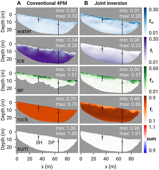
Figure 4. Resulting phase fractions and their sum for the Cervinia field site for (A) the conventional 4PM and (B) the PJI (using Archie's law in both cases). Boreholes and associated thaw depths are marked by black lines. Minimum and maximum phase fractions are indicated for each tomogram.

By fixing the porosity in the 4PM, the near-surface low velocities (cf. Figure 2D) result in a high air content (f_a > 1), which is compensated by a negative ice content (f_i < 0) to satisfy Equation (1). As demonstrated by Wagner et al. (2019), non-physical values are avoided in the joint inversion by the combined use of logarithmic barriers and the volume conservation constraint in Equation (9). In the conventional 4PM case, the thaw layer is well-delineated around borehole SH, but positive ice contents are estimated around borehole DP (Figure 4A). In contrast, the PJI generates only physical values by allowing the porosity to vary within a large range of values during the inversion, resulting in large near-surface lateral variations in porosity and identifying a low porosity zone (high rock content) around borehole DP (corresponding to a weathered bedrock outcrop visible at the surface, Figure 4B).

Moreover, below 10 m depth, the high P-wave velocities lead to a negative air content in the conventional 4PM. A striking feature is the large difference of ice content estimation by the 4PM and PJI, which is a consequence of the fixed rock content in the 4PM case: the fixed pore volumes cause nearly ice-saturated conditions. On the contrary, the PJI estimates a higher rock content (lower porosity) at depth and around borehole DP, which leads to a much lower total ice content estimation. By estimating the rock content within the joint inversion, all estimated pore fractions are considered to be more realistic [e.g., the near-surface air content ~0.5 (PJI) is more realistic than > 1 (4PM)].

Note that by definition, the sum of the four fractions is exactly one in the 4PM case (as Equation 1) is part of the system of equations), whereas it is only close to one for the joint inversion (Figure 4B), as its difference to one is minimized within the objective function (see also sections 2.3 and 4.3). Note as well that the regions where the 4PM gives non-physical solutions (i.e., in the lower part where f_a < 0 and at the surface where f_i < 0, cf. Figure 4A) are corresponding to the regions where the rock content seems problematic in the PJI case without a-priori constraint (cf. Figure 3A).

4.3. Choice of Regularization Parameters

As for every inversion scheme in general, also the results of the PJI highly depend on the choice of regularization parameters (e.g., Mead and Hammerquist, 2013; Zaroli et al., 2013). The higher the regularization (parameters), the smaller is the weight of the observed data during the minimization of the objective function (Equation 10), as more weight will be given to the minimization of the regularization terms (e.g., resulting in smoother results). An analysis of the regularization parameters α, β, and zWeight was performed for all profiles by applying a wide range of values for each regularization parameter to determine the most adequate values, as explained and illustrated in the following for the Cervinia field site and using Archie's law (Figures 5–7). Anisotropic smoothing (i.e., vertical anisotropic smoothness zWeight ≠ 1) is a method to enhance horizontal or vertical structures. The use of a low constraint weight for vertical boundaries (e.g., zWeight < 0.5) is a common technique to improve the inversion results for predominantly layered structures (Günther and Rücker, 2019). Choosing a low value of zWeight would decrease the overall smoothness and may lead to an overfitting of small-scale anomalies. This can be compensated by increasing the smoothness regularization parameter α. To account for this interdependency we therefore simultaneously tested pairs of α and zWeight to determine their most adequate values.

FIGURE 5

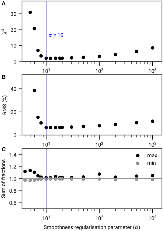
Figure 5. Scatter plot of the smoothness regularization parameter α against (A) χ², (B) RMS, and (C) minimum and maximum sum of the four fractions to determine the most adequate value of α for the Cervinia field site (for constant β and zWeight).

Classical inversion tools are used to assess the data misfit, such as the RMS (in %), which gives an error estimation of the model (Loke and Barker, 1996), or the dimensionless error-weighted χ² mathematical criterion (Günther et al., 2006). χ² is a measure of how well the model fits the data for a given data error (χ² = 1 means a perfect fit of the data within a given error level, Günther and Rücker, 2019). According to Günther et al. (2006), χ² values around 1–5 show reliable results avoiding data overfit or underfit, while Audebert et al. (2014) considers χ² up to 10 giving reliable results.

Joint inversion results have inherent uncertainties due to the non-uniqueness of the solution, i.e., several models can fit the data similarly well within the given error range. As data errors are rarely known accurately and were in our case not measured (through standard methods, such as e.g., reciprocal measurements for ERT, LaBrecque et al., 1996), we had to estimate them carefully. Underestimating the data errors would prevent the inversion to converge (i.e., no solution would be found with underestimated data errors), while overestimating the data errors would prevent the lowest possible data misfit (i.e., prevent obtaining the best possible subsurface image). The individual inversion errors of both data types are used as first guess data errors (err_tt and err_ρa). After the PJI run, the RMS and χ² of each data type are analyzed and are the base of a potential re-evaluation of the data error estimation in order to reduce the discrepancy between input data error and PJI-resulting RMS for each data type. For instance, if χ² < 1, a lower data error is set according to PJI-resulting RMS of the data type considered.

Figures 5A,B show the variation of the resulting χ² and RMS for different values of the smoothness regularization parameter α. For increasing α, both χ² and RMS decrease until a minimum, before increasing again. The α value resulting in the lowest χ² and RMS values, which also corresponds to the most coherent sum of all fractions (closest to one, Figure 5C) is therefore considered the most appropriate. Within the range of acceptable α values (between 10 and 50 in this example), the influence of α on the ice content was found to be negligible (not shown).

Similarly, Figure 6 analyses the influence of the volume conservation regularization parameter β on χ², RMS, and the sum of fractions. Both χ² and RMS gently increase with increasing β, until a threshold is reached, after which both χ² and the RMS start to increase significantly (see Figures 6A,B). Therefore, β should be chosen low enough to minimize χ² and RMS, but also high enough to satisfy Equation (1) (see Figure 6C).

FIGURE 6

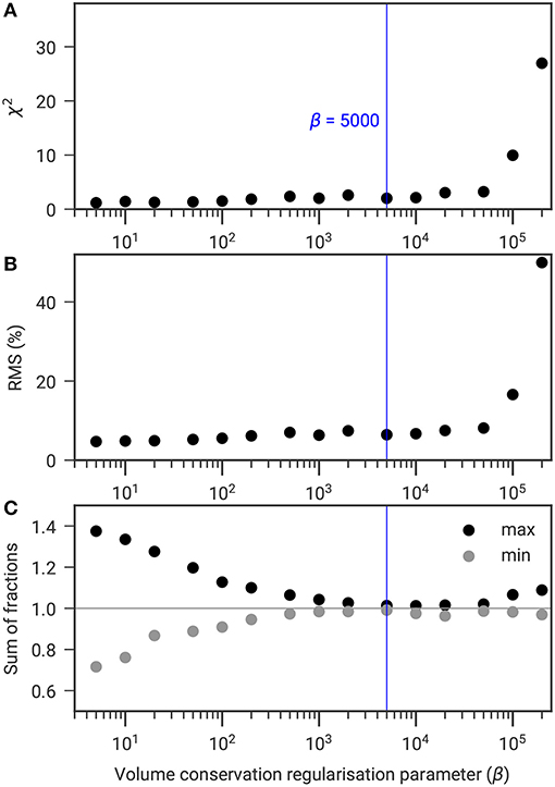
Figure 6. Scatter plot of the regularization parameter β constraining the sum of fractions to be unity against (A) χ², (B) RMS, and (C) minimum and maximum sum of the four fractions to determine the most adequate value of β for the Cervinia field site (for constant α and zWeight).

Figure 7 analyses the influence of the vertical anisotropic smoothness zWeight on χ², RMS, and the sum of all fractions. For increasing zWeight, both χ² and RMS decrease until a minimum, before increasing again (Figures 7A,B). Minimum values of χ² and RMS also correspond to a sum of fractions close to one (Figure 7C).

FIGURE 7

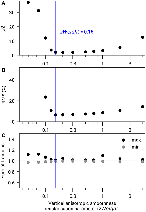
Figure 7. Scatter plot of the vertical anisotropic smoothness parameter zWeight against (A) χ², (B) RMS, and (C) minimum and maximum sum of the four fractions to determine the most adequate value of zWeight for the Cervinia field site (for constant α and β).

The use of anisotropic smoothing to account for observed horizontal layering is often adopted especially for sedimentary formations. Very high regularization anisotropy up to a ratio 1:100 are adopted in the literature (e.g., Attwa and Günther, 2013; Binley et al., 2016). In our case, the application of anisotropic smoothing has the aim to better delineate the active layer by allowing a sharp transition in the ice content and other ground constituents. Resulting zWeight used within the PJI amount to 0.1–0.2 for our field sites (see Table 2).

To sum up, a careful determination of the regularization parameters is essential for the inversion convergence. β has to be chosen to minimize the sum of fractions, while the smoothness regularization parameters should be chosen to minimize χ² or RMS (if the input data errors are adequately chosen, the minimum of both χ² and RMS correlate).

4.4. Comparison of Different Petrophysical Relationships

For all runs of the joint inversion, the selected input parameters correspond to the lowest associated χ² and RMS (i.e., the best possible fits of the model with the data) and the regularization parameters were determined as described in section 4.3. Porosity constraints were chosen according to site geomorphology understanding and are identified in the respective figures. For the rock glaciers, in which ice supersaturation may occur, the porosity is only physically-constrained (i.e., 0 ≤ ϕ ≤ 1), and the starting porosity model is fixed to 0.6. Table 2 summarizes all relevant input parameters for all field sites.

Figure 8 shows a comparison of the PJI results for the four different electrical petrophysical models (described in section 2.2) for the Doldenstock profile. For better comparability, we show the results as virtual borehole logs taken from the respective points on the profile, where boreholes DOL1 and DOL2 are located. Similarly for all petrophysical models, water and air contents generally decrease from about 10 and 50% at the surface to close to zero with depth, respectively (Figure 8). Using model G, the water content diverges from the other models within the first meters (0–3 m depth) at DOL2 and reaches values as high as 30%, which seems overestimated, especially in combination with a high air content (i.e., f_w ~ 30% and f_a ~ 40% at the permafrost table). Results for the water content seem more realistic for models A, A+, and D, while the air content is considered to be well-resolved within the thaw layer, as all different petrophysical models (based on different physical conduction processes) give similar results. One explanation may be that the air content is mostly constrained by the common time-average equation (Equation 2).

FIGURE 8

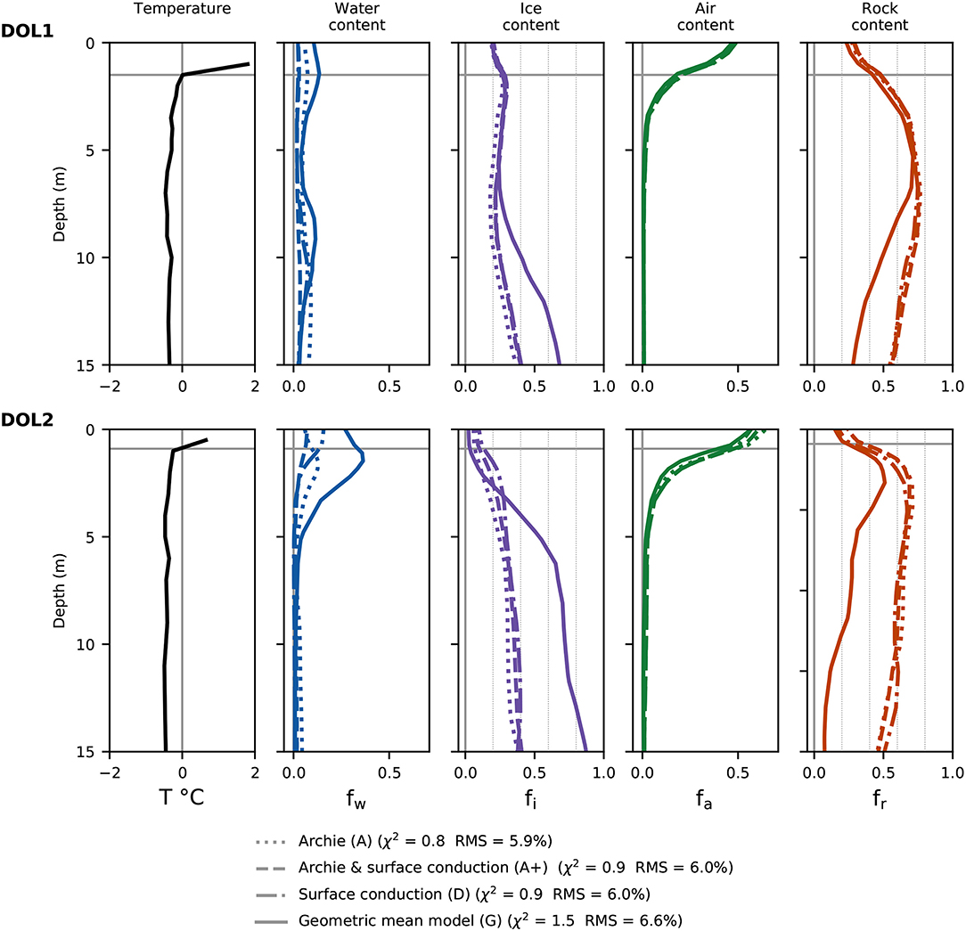
Figure 8. Borehole temperature measured in boreholes DOL1 and DOL2 and corresponding four-phase constituents estimated by the joint inversion with different petrophysical models A, A+, D, and G for the Doldenstock profile. 0°C temperature lines and thaw depths are marked by gray lines.

Rock and ice contents are also similar for all models close to the surface at DOL1 (and to a lesser extent at DOL2), whereas model G diverges from the three others at depth. Only model G detects a large difference in ice and rock contents between the two boreholes, e.g., at 7 m depth, where f_r ~ 0.7 and f_i ~ 0.25 are found for DOL1 (bedrock), while f_r ~ 0.3 and f_i ~ 0.7 are found for the rock glacier material at DOL2 (see Figure 8). The ice content is hereby (realistically) estimated to be minimal in the thaw layer. Hereby, values close to zero are found for model G in DOL2 and slightly overestimated values around 10% for the other models (the PJI resolution capacity is further addressed in section 4.5).

Note that the joint inversions using the geometric mean model (G) were run with a large number of combinations of resistivity of each individual phase (ρ_w, ρ_i, ρ_a, and ρ_r standing for the resistivity of water, ice, air, and rock matrix, respectively) within the standard ranges found in the literature (e.g., Hauck and Kneisel, 2008) for all sites. Almost all of these runs led to unstable inversions (not shown) characterized by very high χ² values (>100 or 1,000), i.e., no convergence. An adequate determination of the resistivities of the four phases is challenging and may prevent a reliable model parameter estimation. The above discussed Doldenstock results (Figure 8) are one of the few examples, where the joint inversion using model G actually converged. The material properties ρ_i and ρ_a are not expected to be site-specific and are found to be similar for all sites (see Table 2). Contrary to the 4PM, where it was found that the parameter ρ_w may have a large influence on the resulting ice contents, small variations in ρ_w in the model G did not influence significantly the overall model parameter estimation (tested ρ_w values were in any case of several orders of magnitude lower than all three other constituents) (see Table 2). Note that the model G always leads to slightly higher χ² and RMS values (see Table 2), because as model G exerts a stronger constrain on the model parameters, the data misfit cannot be as low as in the case of the less constraining models A, A+, or D.

While the reliability of models A, A+, and D relies on a good initial porosity estimate, model G offers constraints for all four phases (as for the time-average seismic equation). In contrast, the resistivity models A, A+, and D constrain only the water content for a given porosity. This may theoretically imply a higher reliability for model G as all four phase contents are constrained by both geophysical datasets. However, the adequate determination of the resistivities of the four phases is challenging (see also the strongly restricted solution space for model G compared to A in the Supplementary Material) and may prohibit meaningful PJI results.

4.5. Ice Content Estimation Comparison With Ground Truth

Previous quantification of ice content exists at Murtél (through core density measurements and direct observations, Haeberli et al., 1988) and at Lapires (through nuclear well logging, see section 3.2.2, Scapozza et al., 2015). Figures 9–11 show the PJI results for MCO, LAH, and LAV, respectively as virtual boreholes in comparison with these ice content estimations.

FIGURE 9

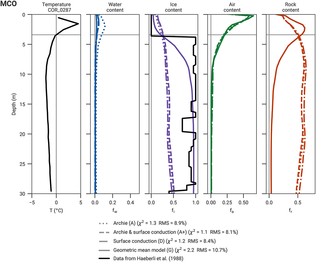
Figure 9. Borehole temperature measured in COR_0287 and corresponding four-phase constituents estimated by the joint inversion for the Murtél profile. The ice content data derived from density measurements (Haeberli et al., 1988) is included. 0°C temperature lines and thaw depths are marked by gray lines.

4.5.1. Murtèl Case

Figure 9 shows the borehole temperature as well as the PJI results for all four phases in comparison with the ice content estimated from the core density measurements in borehole COR_0287 (Haeberli et al., 1988) at Murtél. For all four resistivity petrophysical models the minimum and maximum porosity constraints were set to 0 and 1, and the start porosity was set to 0.6. All four resistivity petrophysical models yielded similar χ² and RMS values (see details in Figure 9 or Table 2). An ice content of roughly 95% (i.e., similar to the validation data) was only estimated when the geometric mean model was considered, whereas the three other resistivity models (A, A+, and D) exhibit largely comparable results, but which do not match the validation data. The upper boundary of the massive ice core (known from the validation data) was however not well-resolved by model G (due to resolution capacity further discussed in section 5.2).

Models A, A+, and D mainly constrain the water content (cf. the respective equations in section 2.2) and are subject to ice-rock ambiguity (Hauck et al., 2011). This ambiguity manifests itself by yielding similarly low RMS errors for a large range of different ice-rock combinations (e.g., for 100% ice, 100% rock, or 50/50% ice/rock). As the RMS depends more on the rock and ice sum, than on the ice-to-rock ratio for certain resistivity-velocity pairs (i.e., high resistivities 10⁵ − 10⁶Ωm, and medium velocities 3,000–4,000 m/s), this ambiguity leads to solutions, which favor ice contents, which are close to the start porosity model. PJI runs considering models A, A+, and D with a higher start porosity (not shown) therefore led to significantly higher estimated ice contents, however, in this case ice contents were also erroneously increased in the unfrozen thaw layer.

Thus, for the case of the massive ice occurrence in Murtél rock glacier, models A, A+, and D do not well constrain the inversion and lead to a large start porosity dependence. On the contrary, the geometric mean model G, which succeeds to correctly estimate the ice content and the air-filled blocks in the thaw layer according to the validation data, seems the most realistic and reliable petrophysical model for Murtél. Moreover, the inflection point of the ice content estimation curve fits well the ice content validation data (see Figure 9).

4.5.2. Lapires Case

Figures 10, 11 show the comparison between the borehole analysis of Scapozza et al. (2015) and the joint inversion results of the profiles LAH and LAV at the location of the boreholes LAP_1108 and LAP_1208, respectively. All four petrophysical models in Figures 10, 11 show overall similar results with the lowest ice content estimate for model A and the highest ice content estimate for model G.

FIGURE 10

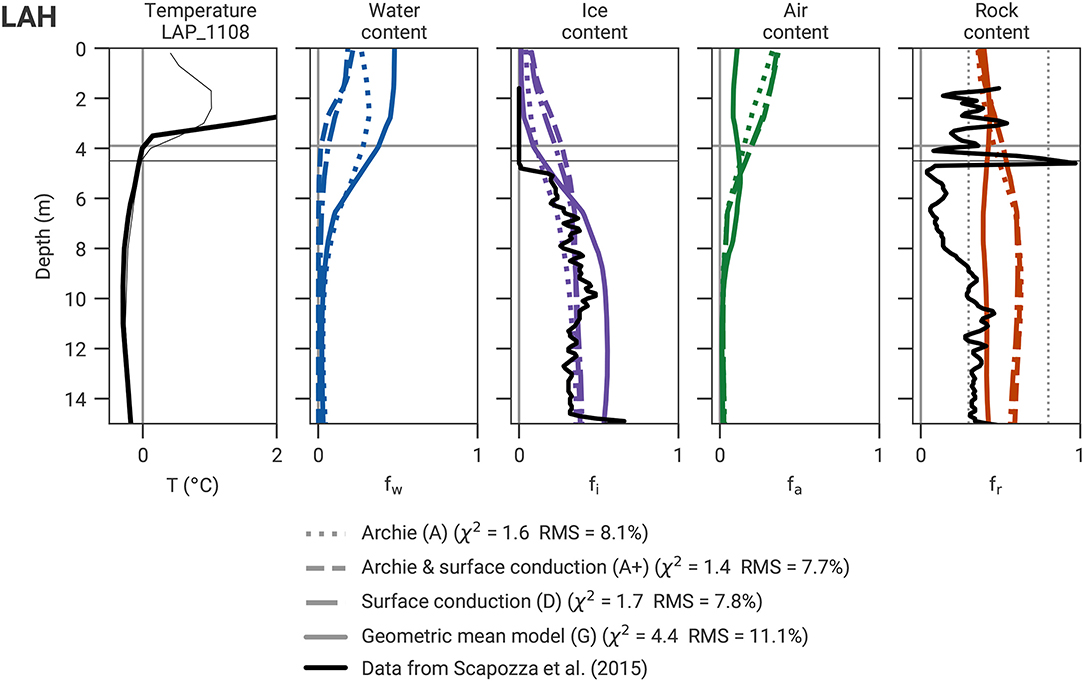
Figure 10. Borehole temperature measured in LAP_1108 and corresponding four-phase constituents estimated by the joint inversion of LAH, including the corresponding data derived from nuclear logging performed by Scapozza et al. (2015) at Lapires. 0°C temperature lines and thaw depths are marked by gray lines, respectively (23 August 2010, date of geophysical surveys). The black horizontal lines as well as the thin temperature curve correspond to the date of the nuclear logging data (30 September 2010). Vertical dotted lines mark the rock constraint limits (from the prescribed porosity range).

FIGURE 11

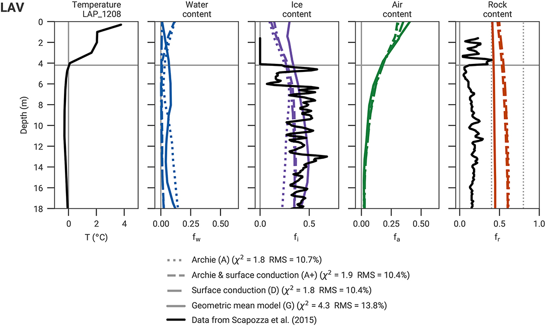
Figure 11. Borehole temperature measured in LAP_1208 and corresponding four-phase constituents estimated by the joint inversion of LAV, including the corresponding data derived from nuclear logging performed by Scapozza et al. (2015) at Lapires. 0°C temperature lines and thaw depths are marked by gray lines. Vertical dotted lines mark the rock constraint limits (from the prescribed porosity range).

For both borehole locations, the ice content estimated from the PJIs is in the range of the mean nuclear logging-derived ice content (except for model G at LAH, Figure 10, and for model A at LAV, Figure 11). As the PJI relies on the spatial resolution of both geophysical methods, its resolution is much smaller than the resolution of typical logging techniques. For this reason and due to the use of smoothness regularization, the joint inversion cannot image local minima and maxima in the ice content, as visible in the well logs. Radioactive logging data also have uncertainties due to calibration processes, the small radius of measurements, and in the case of Lapires, due to the gap in time between the date of drilling and the date of logging (water freezing along the casing may have occurred in between, Scapozza et al., 2015). However, the validation rock and ice content data are derived from independent logging methods, gamma-gamma and neutron-neutron, respectively. Because of higher uncertainties in the rock content and because of the extremely low rock content estimates (reaching only 10% in certain regions), the nuclear logging-derived rock content was considered less reliable than the ice content validation data (Scapozza et al., 2015). The PJI ice content estimation for Lapires corresponds well to the average values derived from the neutron-neutron log (Scapozza et al., 2015), whereas the rock estimation differs significantly (Figures 10, 11).

The overestimated surface water content and underestimated surface air content from model G at the coarse-blocky LAH site (i.e., 50% water, Figure 10) are not due to unreliable PJI estimates, but rather stem from the concrete chairlift pylon foundation which is characterized by a high electrical conductivity (see LAH ERT in Figure 2B). The combination of the resulting small resistivity and small P-wave travel times is then translated into low air content (corresponding to small travel times) and high water content (corresponding to small resistivities) estimations in the PJI.

In contrast to Murtél, where the rock content estimation depends very much on the start porosity value and is overestimated at depth for models A, A+, or D (supersaturated rock glacier, Figure 9), the rock content estimation at Lapires (frozen but not supersaturated talus slope, cf. Figures 10, 11) from the PJI seems more realistic than the corresponding well logging estimates (20% rock content on average is considered an underestimation in both Lapires boreholes).

In summary, the PJI ice content estimation is in general in good agreement with the validation data for the cases of Murtél and Lapires, when different resistivity models are considered, however, with less spatial resolution due to the methodological differences. For the models A, A+, or D, the porosity constraints have a strong influence on the results and need therefore to be chosen carefully according to the field site understanding, while the resistivity of the four phases need to be chosen in case of using model G.

5. Discussion

5.1. Benefits and Limitations of the Approach

5.1.1. Porosity Estimation

It was shown, that, similar to the conventional 4PM, the PJI results are sensitive to the porosity constraints (cf. Figure 3). The more a priori knowledge is available, the better the results can be constrained or validated by independent datasets. One of the limitations of the petrophysical models (and therefore the PJI) comes from the similar resistivity and P-wave velocity ranges characterizing both ice and rock matrix, which leads to a difficult distinction between rock and ice and consequently also results in a wide range of possible porosities (as demonstrated by Hauck et al., 2011). Nevertheless, a heterogeneous porosity seems to be correctly detected in the cases of CER, DOV, and MCO, while no prominent spatial variability of the porosity was expected in the Lapires talus slope. A moderate rock content was correctly found in the MCO surface layer, in contrast to the much lower values in the massive ice core. Despite the ambiguity mentioned above, the petrophysical joint inversion performs well regarding the distinction between ice and rock in cases where either low resistivity occurs with medium velocity (cf. the thaw layer of CER, Figure 2D) or where medium resistivity occurs with high velocity (cf. right part of DOV, Figure 2E).

Other (conventional 4PM) approaches used a prescribed linear porosity decrease with depth (e.g., Schneider et al., 2013) which may, however, be quite wrong for high porosity sites (rock glaciers and talus slopes). To better determine the porosity within the 4PM, Pellet et al. (2016) applied a three-phase model, where the ice content is assumed to be zero. With one model parameter less, the porosity can be directly determined from the three-phase model in the thaw layer. The porosity model resulting from the three-phase model (still including a gradient model for depths below the user-defined thaw layer) was then used as input in the 4PM and showed realistic results regarding the lateral variation of near-surface porosity in the case of Cervinia. The overall estimated porosity values in the thaw layer are comparable to our PJI-derived estimations. Nevertheless, Pellet et al. (2016) found also non-physical values (probably due to the slightly underestimated porosity at depth), which had to be discarded from interpretation (cf. Figure 4). Consequently, the PJI-derived porosity estimation is considered an important improvement, because of its degree of freedom during the determination, even if uncertainties remain in certain cases (i.e., for certain resistivity-velocity pairs).

While we consider the need of having a certain geological and geomorphological understanding to estimate a reasonable porosity start value an important requirement, we are convinced that a PJI based on geophysical methods should not require borehole availability. Boreholes are still expensive and rare in permafrost regions (especially in mountainous regions, Biskaborn et al., 2019), and we believe that geophysical methods (and PJIs) can be applied and bring useful information also where no borehole exists.

5.1.2. Petrophysical Models

We investigated several electrical petrophysical models, but the reliability of the time-average equation [linking the velocities with the volumetric fractions, Equation (2)] was not explored. Other velocity models would also be worth to be investigated (e.g., Draebing and Krautblatter, 2012), especially models which are considering the velocity (and resistivity) as a function of temperature (Carcione and Seriani, 1998; Oldenborger and LeBlanc, 2018), which is quite relevant in a permafrost context, although potentially less relevant for the field sites presented in this study due to their small observed permafrost temperature range (~2–3°C).

For the electrical petrophysical models, the proof-of-concept study was conducted using the classical Archie's law (Wagner et al., 2019). In our study, we tested Archie's law using different values of the Archie parameters m and n, however, many of those parameter combinations resulted in comparably low χ² and RMS values, leading to difficulties to favor one parameter value over another. For this reason, we did not focus on the determination of specific Archie parameters for each site (which may in addition vary spatially), but preferred to compare Archie's law with standard parameters to other petrophysical relationships (similar to e.g., Revil, 2013, who used the approximation m = n = 2). Furthermore, several studies reported the complexity to determine the Archie's parameters even at laboratory scale (e.g., Glover, 2010; Hamada et al., 2012).

The PJI results using the different electrical petrophysical relationships of models A, A+, and D were found to be similar, although their underlying conduction principles are theoretically very different. This can be explained by the inherent uncertainties of the material-dependent values of the free parameters in the various equations [i.e., the Archie parameters in Equation (3), ε in Equation (4), and b in Equation (6)]. The lack of laboratory data from samples from all depths and regions of our field sites made it necessary to prescribe all the above material-dependent properties in order to minimize the joint inversion objective function. These three equations are mainly and directly constraining the water content and porosity, in contrast to the geometric mean model G, which constrains all four fractions. The use of model G within the joint inversion overdetermines the model parameters (all four fractions are constrained by both datasets), while the use of the three other resistivity models led to underdetermined model parameters. This is the reason why the porosity start model has such a large weight on the results when using resistivity models A, A+, or D.

Model G performs differently for the different profiles. It seems to overestimate the ice content at some profiles (i.e., Lapires), while it is the only resistivity model, which recognizes a high porosity without explicitly forcing it (e.g., Murtèl). Model G is therefore the only resistivity model to remarkably lower the ice-rock ambiguity.

5.2. Considerations for Field Applications

The results of the joint inversion of geomorphologically different sites reveal the possibility to distinguish between ice-poor and ice-rich permafrost conditions, and to quantify these differences in ice content values, ranging from average values of 5% up to 95%. Figures 12, 13 show the best-guess ice content distribution estimated for all study sites of this paper as well as the Schilthorn (SCH) site investigated in the proof-of-concept study by Wagner et al. (2019). These results were obtained using the respective resistivity model with the highest confidence, based on the validation data.

FIGURE 12

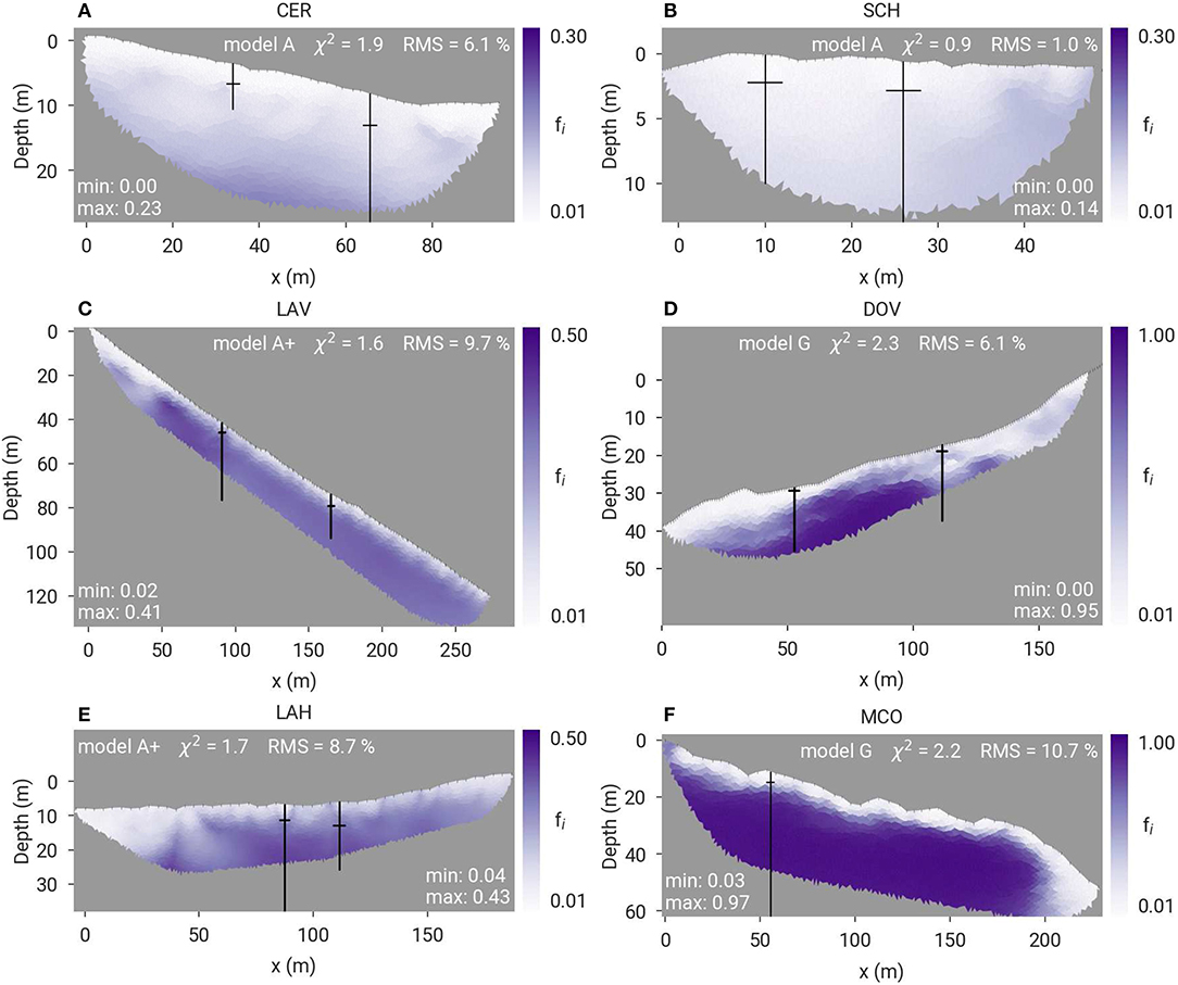
Figure 12. Summary of best-guess ice content distribution for all study sites: (A) CER, (B) SCH (after Wagner et al., 2019), (C) LAV, (D) DOV, (E) LAH, and (F) MCO according to the resistivity model with the highest confidence, respectively (indicated in each panel). Note the different color scales. Minimum and maximum estimated ice content as well as the RMS are also indicated in each panel. Boreholes and associated thaw depths are marked by black lines.

FIGURE 13

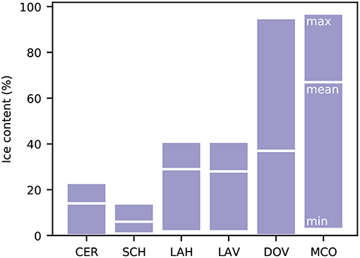
Figure 13. Minimum, mean, and maximum estimated ice content for the entire tomogram of all six sites considering the electrical resistivity models indicated in Figure 12.

Cervinia and Schilthorn hereby represent ice-poor bedrock situations (Figures 12A,B), where low bedrock porosity limits the occurrence of high ice contents. The ice content is found to be larger at CER than at SCH, which correlates to lower ground temperatures observed at CER (Pogliotti et al., 2015; PERMOS, 2019b) probably leading to a higher ice-to-water ratio at Cervinia.

The PJI-estimated ice distributions for the Lapires talus slope (Figures 12C,E) reveal frozen and unfrozen regions (unfrozen on the left-hand side of both profiles), which is in good agreement with the findings of Staub et al. (2015), who used purely temperature-based methods (ground surface and borehole temperatures). The geophysics-based PJI can, however, not resolve the high vertical ice content variability found by borehole studies (e.g., Scapozza et al., 2015), and small, individual ice lenses can therefore not be detected.

For the two rock glacier sites, the PJIs estimate a homogeneously high ice content at MCO (Figure 12F), and a more heterogeneous distribution at DOV (Figure 13), representing correctly both (ice-rich) rock glacier and (ice-poor) bedrock parts of the profile revealed during the drilling (Hilbich et al., 2019). The right-hand side of the profile DOV (Figure 12D), corresponds to high velocities (6000-7300 m/s) resulting in a high rock content (~90%).

The application of the resistivity geometric mean model G led to different performance for the different profiles. The solution space is indeed much narrower for the geometric mean model than for the three other models (such as Archie's law for instance, cf. Figures S1, S2), which can lead to a strongly differing performance depending on the resistivity-velocity pairs.

If an explicit spatial constraint on the thaw layer is not applied (as e.g., described by Wagner et al., 2019), the thaw layer is often only poorly defined (i.e., regions with positive borehole temperature do not necessarily result in a zero ice content). Of course, the PJI resolution capacity is directly driven by the resolutions of the input geophysical data. According to Mewes et al. (2017), a coarse sensor spacing (up to 8 m in our cases) may also lead to poor spatial resolution of small-scale anomalies, which may be improved by smaller electrode and geophone spacings. However, for all presented profiles, the sensor spacing was not chosen to focus on the thaw layer. The case of Cervinia in Figures 3, 4 shows hereby a comparatively good fit of the ice content with the thaw depths, and this profile has also the smallest sensor interval, cf. Table 1).

The resolution as well as the spatial coverage of the data sets (input of the petrophysical joint inversion) may differ significantly and is a further source of uncertainty. Both geophysical methods are indeed sensitive to different physical properties (ERT is particularly sensitive to conductive regions, whereas RST is sensitive to solid phases). This difference in sensitivity is both a strength (complementarity of the methods) and an inconvenience (difference in resolution).

6. Conclusions

A new petrophysical joint inversion (PJI) scheme based on electrical resistivity and refraction seismic tomography data was applied to five permafrost field profiles to estimate the near-surface water, ice, air, and rock distributions in two dimensions. The main findings from this study are:

• The results confirmed that the PJI approach is applicable for very different permafrost landforms, with ice contents varying from low to high volumetric contents. The warranty of physically-plausible solutions and the inclusion of the rock content as part of the output of the joint inversion are significant advantages over the conventional four-phase model. The porosity constraints can, however, significantly influence the results and need therefore to be set carefully according to the field site understanding in order to minimize the uncertainties. Furthermore, a careful determination of data errors and suitable regularization parameters is an essential prerequisite for a reliable model parameter estimation (otherwise the inversion may not converge).

• Water and air contents are well-constrained by the joint inversion scheme, whereas ambiguities between rock and ice contents remain for certain combinations of resistivity-velocity pairs. Rock and ice contents are best resolved when the measured P-wave velocity is relatively low (cf. CER, weathered bedrock occurrence) or high (cf. DOV, bedrock occurrence). The lack of contrast in velocity for ice and rock material is an inherent limitation of the geophysical method (but not due to the joint inversion scheme itself).

• The thaw layer can mostly be identified by its minimal ice content values, but the joint inversion fails to produce zero ice contents in regions with positive temperatures without forcing the presence of a sharp interface. This is partly due to the coarse sensor spacing and corresponding low resolution (note that the thaw layer was best delineated in the case of smallest sensor spacing at Cervinia). The applied smoothing (to stabilize the inversion) does also prevent the detection of strong contrasts.

• The application of Archie's law and the two models taking into account the surface conduction yield largely comparable results, although they are based on theoretically different electrical conduction processes. This can be explained by the lack of field calibration of the respective electrical material parameters included in the equations (e.g., the cation exchange capacity and the pore water resistivity), and the fact that theses parameters are similarly determined by minimizing the data misfit.

• The resistivity geometric mean model G is the most computational demanding of the four models, due to the need to find combinations of the four phase resistivities leading to PJI convergence. In the case of a dry rock glacier, model G led to a drastically reduced ice-rock ambiguity. Theoretically, model G can, therefore, be more reliable because all four phase contents are constrained by both geophysical datasets, but it can only be applied to a narrow range of combinations of resistivity-velocity pairs (narrower solution space, which depends in addition on the velocities and resistivities of the four phases). The use of the resistivity geometric mean model resulted in realistic and well-constrained estimation of the ice content and porosity at Murtél rock glacier.

• The PJI is able to resolve ice-poor to ice-rich conditions. The ice content was found to be 5–15% at the bedrock sites, 20–40% at Lapires talus slope, and up to 95% at Murtèl and Doldenstock rock glaciers. The good correlation with the available and independent ground truth data (thaw depth and ice content) demonstrates the high potential of the joint inversion approach. In addition, geophysical surveys provide additional spatial dimension(s), and allow an additional temporal dimension.

Further developments of the petrophysical joint inversion could include:

• A time-lapse joint inversion constraining the rock content being constant with time could be a significant improvement of the method for the sites having both resistivity and P-wave velocity monitoring data available (e.g., SCH or LAH, cf. Hilbich, 2010; Hauck et al., 2017; Mewes et al., 2017). The assumption of a constant rock content with time (in case of absence of excess ice, i.e., not applicable for e.g., rock glaciers) would reduce the number of model parameters and thereby decrease the uncertainties. The determination of temporal ice content changes has therefore a potential of higher reliability (Hauck et al., 2017).

• The addition of (an)other geophysical dataset(s) into the petrophysical model. For instance, induced polarization (Doetsch et al., 2015; Duvillard et al., 2018) and spectral induced polarization studies (Wu et al., 2017) confirmed in laboratory experiments that polarization signals can differentiate between frozen and unfrozen states.

• Integrating non-geophysical data in the petrophysical joint inversion (as done with the thaw depth by Wagner et al., 2019) could be further explored using e.g., the well logging data as structural constraints (e.g., Giraud et al., 2017; Heincke et al., 2017; Steiner et al., 2019). Another physical constraint may consist in penalizing non-physical cases where the sum of f_w and f_a is higher than a certain threshold (e.g., 0.5).

• More site specific field measurements of the pore water resistivity or cation exchange capacity (Duvillard et al., 2018; Coperey et al., 2019) for instance may help to better constrain the petrophysical model (although representative values for the whole profile and all depths are sometimes difficult to obtain).

Moreover, a probabilistic Monte-Carlo approach may help to determine the most appropriate petrophysical model.

Data Availability Statement

The field data as well as scripts to reproduce results and figures of the paper can be obtained through the corresponding author. The joint inversion code itself is freely available at https://github.com/florian-wagner/four-phase-inversion.

Author Contributions

CM performed the PJI modeling, data analysis, and interpretation. FW developed the main PJI code based on conceptual discussions with CM and CHa. CM designed the manuscript with contributions of FW, CHi, and CHa. CM, CHi, CS, and CHa contributed to the data collection. All authors contributed to the results, discussion, and the manuscript revision.

Funding

This study was conducted within two projects funded by the Swiss National Science Foundation (SPICE, 200021L_178823 and MODAIRCAP, 200021_169499).

Conflict of Interest

The authors declare that the research was conducted in the absence of any commercial or financial relationships that could be construed as a potential conflict of interest.

Acknowledgments

We were grateful to the PERMOS office, our colleagues from ARPA (Italian Regional Environmental Protection Agency), and Nils Hählen (Office of Forest and Natural Hazards of the Canton of Bern, Switzerland) for providing the temperature data and supporting the geophysical field work. We were thankful to the cable car companies Télénendaz S.A., Schilthornbahn and Corvatsch AG for the logistical support to our research activities.

Supplementary Material

The Supplementary Material for this article can be found online at: https://www.frontiersin.org/articles/10.3389/feart.2020.00085/full#supplementary-material

References

Archie, G. (1942). The electrical resistivity log as an aid in determining some reservoir characteristics. Trans. AIME 146, 54–62. doi: 10.2118/942054-G

CrossRef Full Text | Google Scholar

Attwa, M., and Günther, T. (2013). Spectral induced polarization measurements for predicting the hydraulic conductivity in sandy aquifers. Hydrol. Earth Syst. Sci. 17, 4079–4094. doi: 10.5194/hess-17-4079-2013

CrossRef Full Text | Google Scholar

Audebert, M., Clément, R., Touze-Foltz, N., Günther, T., Moreau, S., and Duquennoi, C. (2014). Time-lapse ERT interpretation methodology for leachate injection monitoring based on multiple inversions and a clustering strategy (MICS). J. Appl. Geophys. 111, 320–333. doi: 10.1016/j.jappgeo.2014.09.024

CrossRef Full Text | Google Scholar

Barsch, D., Fierz, H., and Haeberli, W. (1979). Shallow core drilling and bore-hole measurements in the permafrost of an active rock glacier near the grubengletscher, Wallis, Swiss Alps. Arctic Alpine Res. 11, 215–228. doi: 10.2307/1550646

CrossRef Full Text | Google Scholar

Binley, A., Keery, J., Slater, L., Barrash, W., and Cardiff, M. (2016). The hydrogeologic information in cross-borehole complex conductivity data from an unconsolidated conglomeratic sedimentary aquifer. Geophysics 81, E409–E421. doi: 10.1190/geo2015-0608.1

CrossRef Full Text | Google Scholar

Biskaborn, B. K., Smith, S. L., Noetzli, J., Matthes, H., Vieira, G., Streletskiy, D. A., et al. (2019). Permafrost is warming at a global scale. Nat. Commun. 10:264. doi: 10.1038/s41467-018-08240-4

PubMed Abstract | CrossRef Full Text | Google Scholar

Briggs, M., Campbell, S., Nolan, J., Walvoord, M., Ntarlagiannis, D., Day-Lewis, F., et al. (2016). Surface geophysical methods for characterising frozen ground in transitional permafrost landscapes. Permafr. Perigl. Process. 28, 52–65. doi: 10.1002/ppp.1893

CrossRef Full Text | Google Scholar

Buchli, T., Merz, K., Zhou, X., Kinzelbach, W., and Springman, S. M. (2013). Characterization and monitoring of the Furggwanghorn rock glacier, Turtmann Valley, Switzerland: Results from 2010 to 2012. Vadose Zone J. 12, 1–15. doi: 10.2136/vzj2012.0067

CrossRef Full Text | Google Scholar

Carcione, J., Ursin, B. I., and Nordskag, J. (2007). Cross-property relations between electrical conductivity and the seismic velocity of rocks. Geophysics 72, E193–E204. doi: 10.1190/1.2762224

CrossRef Full Text | Google Scholar

Carcione, J. M., and Seriani, G. (1998). Seismic and ultrasonic velocities in permafrost. Geophys. Prospect. 46, 441–454. doi: 10.1046/j.1365-2478.1998.1000333.x

CrossRef Full Text | Google Scholar

Coperey, A., Revil, A., Abdulsamad, F., Stutz, B., Duvillard, P. A., and Ravanel, L. (2019). Low-frequency induced polarization of porous media undergoing freezing: Preliminary observations and modeling. J. Geophys. Res. Solid Earth. 124, 4523–4544. doi: 10.1029/2018JB017015

CrossRef Full Text | Google Scholar

Degenhardt, J. J. (2003). Subsurface investigation of a rock glacier using ground-penetrating radar: Implications for locating stored water on Mars. J. Geophys. Res. 108:8036. doi: 10.1029/2002JE001888

CrossRef Full Text | Google Scholar

Delaloye, R., and Lambiel, C. (2005). Evidence of winter ascending air circulation throughout talus slopes and rock glaciers situated in the lower belt of alpine discontinuous permafrost (Swiss Alps). Norsk Geogr Tidsskr. 59, 194–203. doi: 10.1080/00291950510020673

CrossRef Full Text | Google Scholar

Doetsch, J., Ingeman-Nielsen, T., Christiansen, A. V., Fiandaca, G., Auken, E., and Elberling, B. (2015). Direct current (DC) resistivity and induced polarization (IP) monitoring of active layer dynamics at high temporal resolution. Cold Regions Sci. Technol. 119, 16–28. doi: 10.1016/j.coldregions.2015.07.002

CrossRef Full Text | Google Scholar

Doetsch, J., Linde, N., and Binley, A. (2010). Structural joint inversion of time-lapse crosshole ERT and GPR traveltime data. Geophys. Res. Lett. 37:L24404. doi: 10.1029/2010GL045482

CrossRef Full Text | Google Scholar

Doetsch, J., Linde, N., Pessognelli, M., Green, A. G., and Günther, T. (2012). Constraining 3-D electrical resistance tomography with GPR reflection data for improved aquifer characterization. J. Appl. Geophys. 78, 68–76. doi: 10.1016/j.jappgeo.2011.04.008

CrossRef Full Text | Google Scholar

Draebing, D. (2016). Application of refraction seismics in alpine permafrost studies: a review. Earth Sci. Rev. 155, 136–152. doi: 10.1016/j.earscirev.2016.02.006

CrossRef Full Text | Google Scholar

Draebing, D., and Krautblatter, M. (2012). P-wave velocity changes in freezing hard low-porosity rocks: a laboratory-based time-average model. Cryosphere 6, 1163–1174. doi: 10.5194/tc-6-1163-2012

CrossRef Full Text | Google Scholar

Duvillard, P. A., Revil, A., Qi, Y., Soueid Ahmed, A., Coperey, A., and Ravanel, L. (2018). Three-dimensional electrical conductivity and induced polarization tomography of a rock glacier. J. Geophys. Res. Solid Earth 123, 9528–9554. doi: 10.1029/2018JB015965

CrossRef Full Text | Google Scholar

Emmert, A., and Kneisel, C. (2017). Internal structure of two alpine rock glaciers investigated by quasi-3-D electrical resistivity imaging. Cryosphere 11, 841–855. doi: 10.5194/tc-11-841-2017

CrossRef Full Text | Google Scholar

Federal Office of Topography Swisstopo (2019). Geological Vector Datasets Geocover v2. Available online at: www.map.geo.admin.ch

Friedel, S., Thielen, A., and Springman, S. (2006). Investigation of a slope endangered by rainfall-induced landslides using 3D resistivity tomography and geotechnical testing. J. Appl. Geophys. 60, 100–114. doi: 10.1016/j.jappgeo.2006.01.001

CrossRef Full Text | Google Scholar

Gallardo, L. A., and Meju, M. A. (2003). Characterization of heterogeneous near-surface materials by joint 2D inversion of dc resistivity and seismic data. Geophys. Res. Lett. 30:1658. doi: 10.1029/2003GL017370

CrossRef Full Text | Google Scholar

Gallardo, L. A., and Meju, M. A. (2004). Joint two-dimensional DC resistivity and seismic travel time inversion with cross-gradients constraints. J. Geophys. Res. Solid Earth 109:B03311. doi: 10.1029/2003JB002716

CrossRef Full Text | Google Scholar

Garofalo, F. (2014). Physically constrained joint inversion of seismic and electrical data for near-surface application (Ph.D. thesis), Politecnico di Torino, Italy.

Google Scholar

Garofalo, F., Sauvin, G., Socco, L. V., and Lecomte, I. (2015). Joint inversion of seismic and electric data applied to 2D mediaseismic and electric data joint inversion. Geophysics 80:EN93. doi: 10.1190/geo2014-0313.1

CrossRef Full Text | Google Scholar

Giraud, J., Pakyuz-Charrier, E., Jessell, M., Lindsay, M., Martin, R., and Ogarko, V. (2017). Uncertainty reduction through geologically conditioned petrophysical constraints in joint inversion. Geophysics 82, ID19–ID34. doi: 10.1190/geo2016-0615.1

CrossRef Full Text | Google Scholar

Glover, P. (2010). A generalized Archie's law for n phases. Geophysics 75:E247. doi: 10.1190/1.3509781

CrossRef Full Text | Google Scholar

Günther, T., and Rücker, C. (2019). Boundless Electrical Resistivity Tomography BERT, The User Tutorial. version 2.2.8, 1–70.

Google Scholar

Günther, T., Rücker, C., and Spitzer, K. (2006). Three-dimensional modelling and inversion of dc resistivity data incorporating topography'II. Inversion. Geophys. J. Int. 166, 506–517. doi: 10.1111/j.1365-246X.2006.03011.x

CrossRef Full Text | Google Scholar

Haeberli, W., Huder, J., Keusen, H., Pika, J., and Röthlisberger, H. (1988). “Core drilling through rock glacier permafrost,” in Proceedings of the Fifth International Conference on Permafrost (Trondheim: Tapir Publishers), 937–944.

Google Scholar

Hamada, G. M., Almajed, A. A., Okasha, T. M., and Algathe, A. A. (2012). Uncertainty analysis of Archie's parameters determination techniques in carbonate reservoirs. J. Petrol. Explor. Prod. Technol. 3, 1–10. doi: 10.1007/s13202-012-0042-x

CrossRef Full Text | Google Scholar

Harris, S. A., French, H. M., Heginbottom, J. A., Johnston, G. H., Ladanyi, B., Sego, D. C., et al. (1988). Glossary of Permafrost and Related Ground-Ice Terms. Ottawa, ON: National Research Council of Canada, Associate Committee on Geotechnical Research.

Hauck, C., Böttcher, M., and Maurer, H. (2011). A new model for estimating subsurface ice content based on combined electrical and seismic data sets. Cryosphere 5, 453–468. doi: 10.5194/tc-5-453-2011

CrossRef Full Text | Google Scholar

Hauck, C., Hilbich, C., and Mollaret, C. (2017). “A time-lapse geophysical model for detecting changes in ground ice content based on electrical and seismic mixing rules,” in 23rd European Meeting of Environmental and Engineering Geophysics (Malmö: EAGE Publications BV).

Google Scholar

Hauck, C., and Kneisel, C. (2008). Applied Geophysics in Periglacial Environments. Vol. 240. Cambridge: Cambridge University Press.

Google Scholar

Hausmann, H., Krainer, K., Brückl, E., and Mostler, W. (2007). Internal structure and ice content of Reichenkar rock glacier (Stubai Alps, Austria) assessed by geophysical investigations. Permafr. Perigl. Process. 18, 351–367. doi: 10.1002/ppp.601

CrossRef Full Text | Google Scholar

Heincke, B., Jegen, M., Moorkamp, M., Hobbs, R. W., and Chen, J. (2017). An adaptive coupling strategy for joint inversions that use petrophysical information as constraints. J. Appl. Geophys. 136, 279–297. doi: 10.1016/j.jappgeo.2016.10.028

CrossRef Full Text | Google Scholar

Hellman, K., Ronczka, M., Günther, T., Wennermark, M., Rücker, C., and Dahlin, T. (2017). Structurally coupled inversion of ERT and refraction seismic data combined with cluster-based model integration. J. Appl. Geophys. 143, 169–181. doi: 10.1016/j.jappgeo.2017.06.008

CrossRef Full Text | Google Scholar

Hilbich, C. (2010). Time-lapse refraction seismic tomography for the detection of ground ice degradation. Cryosphere 4, 243–259. doi: 10.5194/tc-4-243-2010

CrossRef Full Text | Google Scholar

Hilbich, C., Fuss, C., and Hauck, C. (2011). Automated time-lapse ERT for improved process analysis and monitoring of frozen ground. Permafr. Perigl. Process. 22, 306–319. doi: 10.1002/ppp.732

CrossRef Full Text | Google Scholar

Hilbich, C., Hauck, C., Hoelzle, M., Scherler, M., Schudel, L., Völksch, I., et al. (2008). Monitoring mountain permafrost evolution using electrical resistivity tomography: a 7-year study of seasonal, annual, and long-term variations at Schilthorn, Swiss Alps. J. Geophys. Res. Earth Surf. 113:F01S90. doi: 10.1029/2007JF000799

CrossRef Full Text | Google Scholar

Hilbich, C., Hauck, C., and Mollaret, C. (2019). Geophysikalische Untersuchungen zur Permafrost-Verbreitung im Berner Oberland, 2015–2018. Fribourg: University of Fribourg.

Google Scholar

Hilbich, C., Marescot, L., Hauck, C., Loke, M. H., and Mäusbacher, R. (2009). Applicability of electrical resistivity tomography monitoring to coarse blocky and ice-rich permafrost landforms. Permafr. Perigl. Process. 20, 269–284. doi: 10.1002/ppp.652

CrossRef Full Text | Google Scholar

Hoelzle, M., Mühll, D. V., and Haeberli, W. (2002). Thirty years of permafrost research in the Corvatsch-Furtschellas area, Eastern Swiss Alps: a review. Norsk Geogr. Tidsskr. 56, 137–145. doi: 10.1080/002919502760056468

CrossRef Full Text | Google Scholar

IPCC (2019). “Summary for policymakers,” in IPCC Special Report on the Ocean and Cryosphere in a Changing Climate, eds H. O. Pörtner, D. Roberts, V. Masson-Delmotte, P. Zhai, M. Tignor, E. Poloczanska, et al. Available online at: https://www.ipcc.ch/srocc/cite-report/

Google Scholar

Karaoulis, M., Tsourlos, P., Kim, J.-H., and Revil, A. (2013). 4D time-lapse ERT inversion: introducing combined time and space constraints. Near Surf. Geophys. 12, 25–34. doi: 10.3997/1873-0604.2013004

CrossRef Full Text | Google Scholar

Kenner, R., Noetzli, J., Hoelzle, M., Raetzo, H., and Phillips, M. (2019). Distinguishing ice-rich and ice-poor permafrost to map ground temperatures and ground ice occurrence in the swiss alps. Cryosphere 13, 1925–1941. doi: 10.5194/tc-13-1925-2019

CrossRef Full Text | Google Scholar

Klein, K. A., and Santamarina, J. C. (2003). Electrical conductivity in soils: Underlying phenomena. J. Environ. Eng. Geophys. 8, 263–273. doi: 10.4133/JEEG8.4.263

CrossRef Full Text | Google Scholar

Kneisel, C., Hauck, C., Fortier, R., and Moorman, B. (2008). Advances in geophysical methods for permafrost investigations. Permafr. Perigl. Process. 19, 157–178. doi: 10.1002/ppp.616

CrossRef Full Text | Google Scholar

Krainer, K., Bressan, D., Dietre, B., Haas, J. N., Hajdas, I., Lang, K., et al. (2015). A 10,300-year-old permafrost core from the active rock glacier Lazaun, southern Ö-tztal Alps (South Tyrol, northern Italy). Quart. Res. 83, 324–335. doi: 10.1016/j.yqres.2014.12.005

CrossRef Full Text | Google Scholar

LaBrecque, D. J., Miletto, M., Daily, W., Ramirez, A., and Owen, E. (1996). The effects of noise on Occam's inversion of resistivity tomography data. Geophysics 61, 538–548. doi: 10.1190/1.1443980

CrossRef Full Text | Google Scholar

Léger, E., Dafflon, B., Soom, F., Peterson, J., Ulrich, C., and Hubbard, S. (2017). Quantification of arctic soil and permafrost properties using ground-penetrating radar and electrical resistivity tomography datasets. IEEE J. Select. Top. Appl. Earth Observ. Rem. Sens. 10, 4348–4359. doi: 10.1109/JSTARS.2017.2694447

CrossRef Full Text | Google Scholar

Linde, N., and Doetsch, J. (2016). “Joint inversion in hydrogeophysics and near-surface geophysics,” in Integrated Imaging of the Earth, eds M. Moorkamp, P. G. Lelièvre, N. Linde, and A. Khan (John Wiley & Sons, Inc.), 117–135. doi: 10.1002/9781118929063.ch7

CrossRef Full Text | Google Scholar

Liu, L., and Larson, K. M. (2018). Decadal changes of surface elevation over permafrost area estimated using reflected GPS signals. Cryosphere 12, 477–489. doi: 10.5194/tc-12-477-2018

CrossRef Full Text | Google Scholar

Loke, M., and Barker, R. (1996). Rapid least-squares inversion of apparent resistivity pseudosections by a quasi-newton method. Geophys. Prospect. 44, 131–152. doi: 10.1111/j.1365-2478.1996.tb00142.x

CrossRef Full Text | Google Scholar

Maurer, H., and Hauck, C. (2007). Geophysical imaging of alpine rock glaciers. J. Glaciol. 53, 110–120. doi: 10.3189/172756507781833893

CrossRef Full Text | Google Scholar

Mead, J. L., and Hammerquist, C. C. (2013). χ² tests for the choice of the regularization parameter in nonlinear inverse problems. SIAM J. Matrix Anal. Appl. 34, 1213–1230. doi: 10.1137/12088447X

CrossRef Full Text | Google Scholar

Menke, W. (1989). Geophysical Data Analysis: Discrete Inverse Theory. Rev. Edn., Vol. 45. San Diego, CA: Academic Press.

Merz, K., Maurer, H., Rabenstein, L., Buchli, T., Springman, S. M., and Zweifel, M. (2016). Multidisciplinary geophysical investigations over an alpine rock glacier. Geophysics 81, WA147–WA157. doi: 10.1190/geo2015-0157.1

CrossRef Full Text | Google Scholar

Mewes, B., Hilbich, C., Delaloye, R., and Hauck, C. (2017). Resolution capacity of geophysical monitoring regarding permafrost degradation induced by hydrological processes. Cryosphere 11, 2957–2974. doi: 10.5194/tc-11-2957-2017

CrossRef Full Text | Google Scholar

Mollaret, C., Hilbich, C., Pellet, C., Flores-Orozco, A., Delaloye, R., and Hauck, C. (2019). Mountain permafrost degradation documented through a network of permanent electrical resistivity tomography sites. Cryosphere 13, 2557–2578. doi: 10.5194/tc-13-2557-2019

CrossRef Full Text | Google Scholar

Monnier, S., and Kinnard, C. (2013). Internal structure and composition of a rock glacier in the Andes (upper Choapa valley, Chile) using borehole information and ground-penetrating radar. Ann. Glaciol. 54, 61–72. doi: 10.3189/2013AoG64A107

CrossRef Full Text | Google Scholar

Oldenborger, G. A., and LeBlanc, A.-M. (2018). Monitoring changes in unfrozen water content with electrical resistivity surveys in cold continuous permafrost. Geophys. J. Int. 215, 965–977. doi: 10.1093/gji/ggy321

CrossRef Full Text | Google Scholar

Parsekian, A. D., Singha, K., Minsley, B. J., Holbrook, W. S., and Slater, L. (2015). Multiscale geophysical imaging of the critical zone. Rev. Geophys. 53, 1–26. doi: 10.1002/2014RG000465

CrossRef Full Text | Google Scholar

Pellet, C., Hilbich, C., Marmy, A., and Hauck, C. (2016). Soil moisture data for the validation of permafrost models using direct and indirect measurement approaches at three alpine sites. Front. Earth Sci. 3:91. doi: 10.3389/feart.2015.00091

CrossRef Full Text | Google Scholar

Pepin, N., Bradley, R., Diaz, H., Baraer, M., Cáceres, B., Forsythe, N., et al. (2015). Elevation-dependent warming in mountain regions of the world. Nat. Clim. Change 5, 424–430. doi: 10.1038/nclimate2563

CrossRef Full Text | Google Scholar

PERMOS (2013). “Permafrost in Switzerland 2008/2009 and 2009/2010,” in Glaciological Report (Permafrost) No. 10/11 of the Cryospheric Commission of the Swiss Academy of Sciences, ed J. Noetzli (Zürich: Cryospheric Commission of the Swiss Academy of Sciences), 80.

PERMOS (2019a). “Permafrost in Switzerland 2014/2015 to 2017/2018,” in Glaciological Report (Permafrost) No. 16-19 of the Cryospheric Commission of the Swiss Academy of Sciences, eds J. Noetzli, C. Pellet, and B. Staub (Fribourg; Davos: Cryospheric Commission of the Swiss Academy of Sciences), 104.

Google Scholar

PERMOS (2019b). PERMOS Database. Swiss Permafrost Monitoring Network, Fribourg and Davos.

Pogliotti, P., Guglielmin, M., Cremonese, E., di Cella, U. M., Filippa, G., Pellet, C., et al. (2015). Warming permafrost and active layer variability at Cime Bianche, Western European Alps. Cryosphere 9, 647–661. doi: 10.5194/tc-9-647-2015

CrossRef Full Text | Google Scholar

Python, S. (2015). Technical improvement of the 4-phase model to better assess the ice, water and air content estimation in permafrost substrates. Case study: Stockhorn, Valais, Switzerland (Master's thesis), Department of Geosciences, University of Fribourg, Fribourg, Switzerland.

Ravanel, L., Magnin, F., and Deline, P. (2017). Impacts of the 2003 and 2015 summer heatwaves on permafrost-affected rock-walls in the Mont Blanc massif. Sci. Total Environ. 609, 132–143. doi: 10.1016/j.scitotenv.2017.07.055

PubMed Abstract | CrossRef Full Text | Google Scholar

Revil, A. (2013). Effective conductivity and permittivity of unsaturated porous materials in the frequency range 1 mHz-1GHz. Water Resourc. Res. 49, 306–327. doi: 10.1029/2012WR012700

PubMed Abstract | CrossRef Full Text | Google Scholar

Revil, A., Barnier, G., Karaoulis, M., Sava, P., Jardani, A., and Kulessa, B. (2014). Seismoelectric coupling in unsaturated porous media: theory, petrophysics, and saturation front localization using an electroacoustic approach. Geophys. J. Int. 196, 867–884. doi: 10.1093/gji/ggt440

CrossRef Full Text | Google Scholar

Ronczka, M., Hellman, K., Günther, T., Wisén, R., and Dahlin, T. (2017). Electric resistivity and seismic refraction tomography: a challenging joint underwater survey at Äspö Hard Rock Laboratory. Solid Earth 8, 671–682. doi: 10.5194/se-8-671-2017

CrossRef Full Text | Google Scholar

Rücker, C., Günther, T., and Wagner, F. M. (2017). pyGIMLi: An open-source library for modelling and inversion in geophysics. Comput. Geosci. 109, 106–123. doi: 10.1016/j.cageo.2017.07.011

CrossRef Full Text | Google Scholar

Sandmeier, K. (2019). REFLEXW Version 9.0 Windows^TM XP/7/8/10-Program for the Processing of Seismic, Acoustic or Electromagnetic Reflection, Refraction and Transmission Data. Available online at: https://www.sandmeier-geo.de/Download/reflexw_manual_a4_booklet.pdf

PubMed Abstract | Google Scholar

Scapozza, C. (2013). Stratigraphie, morphodynamique, paléoenvironnements des terrains sédimentaires meubles á forte déclivité dudomaine périglaciaire alpin. Géovisions 40, Institut de géographie et durabilité de l'Université de Lausanne, Lausanne.

Google Scholar

Scapozza, C., Baron, L., and Lambiel, C. (2015). Borehole logging in alpine periglacial talus slopes (Valais, Swiss Alps). Permafr. Perigl. Process. 26, 67–83. doi: 10.1002/ppp.1832

CrossRef Full Text | Google Scholar

Scherler, M., Hauck, C., Hoelzle, M., and Salzmann, N. (2013). Modeled sensitivity of two alpine permafrost sites to RCM-based climate scenarios. J. Geophys. Res. Earth Surf. 118, 780–794. doi: 10.1002/jgrf.20069

CrossRef Full Text | Google Scholar

Schneider, S., Daengeli, S., Hauck, C., and Hoelzle, M. (2013). A spatial and temporal analysis of different periglacial materials by using geoelectrical, seismic and borehole temperature data at Murtèl-Corvatsch, Upper Engadin, Swiss Alps. Geogr. Helvet. 68, 265–280. doi: 10.5194/gh-68-265-2013

CrossRef Full Text | Google Scholar

Scott, W. J., Sellmann, P. V., and Hunter, J. A. (1990). 13. “Geophysics in the study of permafrost,” in Geotechnical and Environmental Geophysics, ed S. H. Ward (Tulsa, OK: Society of Exploration Geophysicists), 355–384. doi: 10.1190/1.9781560802785.ch13

CrossRef Full Text | Google Scholar

Sen, P. N., Goode, P. A., and Sibbit, A. (1988). Electrical conduction in clay bearing sandstones at low and high salinities. J. Appl. Phys. 63, 4832–4840. doi: 10.1063/1.340476

CrossRef Full Text | Google Scholar

Staub, B., Marmy, A., Hauck, C., Hilbich, C., and Delaloye, R. (2015). Ground temperature variations in a talus slope influenced by permafrost: a comparison of field observations and model simulations. Geogr. Helvet. 70:45. doi: 10.5194/gh-70-45-2015

CrossRef Full Text | Google Scholar

Steiner, M., Wagner, F. M., and Flores-Orozco, A. (2019). Improved characterization of alpine permafrost through structurally constrained inversion of refraction seismic data. Cryosphere Discuss. 1–27. doi: 10.5194/tc-2019-52

CrossRef Full Text | Google Scholar

Timur, A. (1968). Velocity of compressional waves in porous media at permafrost temperatures. Geophysics 33, 584–595. doi: 10.1190/1.1439954

CrossRef Full Text | Google Scholar

Vey, S., Steffen, H., Müller, J., and Boike, J. (2012). Inter-annual water mass variations from GRACE in central Siberia. J. Geodesy 87, 287–299. doi: 10.1007/s00190-012-0597-9

CrossRef Full Text | Google Scholar

Vonder Mühll, D. S., and Klingelé, E. E. (1994). Gravimetrical investigation of ice-rich permafrost within the rock glacier Murtél-Corvatsch (upper Engadin, Swiss Alps). Permafr. Perigl. Process. 5, 13–24. doi: 10.1002/ppp.3430050103

CrossRef Full Text | Google Scholar

Vozoff, K., and Jupp, D. L. B. (1975). Joint inversion of geophysical data. Geophys. J. Int. 42, 977–991. doi: 10.1111/j.1365-246X.1975.tb06462.x

CrossRef Full Text | Google Scholar

Wagner, F. M., Mollaret, C., Günther, T., Kemna, A., and Hauck, C. (2019). Quantitative imaging of water, ice, and air in permafrost systems through petrophysical joint inversion of seismic refraction and electrical resistivity data. Geophys. J. Int. 219, 1866–1875. doi: 10.1093/gji/ggz402

CrossRef Full Text | Google Scholar

Wang, S., Sheng, Y., Li, J., Wu, J., Cao, W., and Ma, S. (2018). An Estimation of Ground Ice Volumes in Permafrost Layers in North-eastern Qinghai-Tibet Plateau, China. Chin. Geogr. Sci. 28:61. doi: 10.1007/s11769-018-0932-z

CrossRef Full Text | Google Scholar

Waxman, M., and Smits, L. (1968). Electrical conductivities in oil-bearing shaly sands. Soc. Petrol. Eng. J. 8, 107–122. doi: 10.2118/1863-A

CrossRef Full Text | Google Scholar

Wu, Y., Nakagawa, S., Kneafsey, T. J., Dafflon, B., and Hubbard, S. S. (2017). Electrical and seismic response of saline permafrost soil during freeze-thaw transition. J. Appl. Geophys. 146, 16–26. doi: 10.1016/j.jappgeo.2017.08.008

CrossRef Full Text | Google Scholar

Zaroli, C., Sambridge, M., Lévêque, J.-J., Debayle, E., and Nolet, G. (2013). An objective rationale for the choice of regularisation parameter with application to global multiple-frequency S-wave tomography. Solid Earth 4, 357–371. doi: 10.5194/se-4-357-2013

CrossRef Full Text | Google Scholar

Zhang, J., and Morgan, F. D. (1997). “Joint seismic and electrical tomography,” in Symposium on the Application of Geophysics to Engineering and Environmental Problems 1997 (Reno: Environment and Engineering Geophysical Society). doi: 10.4133/1.2922412

CrossRef Full Text | Google Scholar