Modeling the Dynamic Landscape Evolution of a Volcanic Coastal Environment Under Future Climate Trajectories

Introduction

Greenhouse gases have been increasing rapidly over the past century and will almost certainly continue to do so into the foreseeable future, in turn effectively impacting global climate (IPCC, 2001). Recently, the idea of introducing negative emissions technologies (NETs) to actively uptake carbon dioxide out of the atmosphere, have been advocated. One approach that has been proposed is enhanced silicate weathering, which is a strategy in which humans could enhance the natural process of mineral weathering (specifically olivine) to such a degree that enough CO₂ could be taken out of the atmosphere to at least partially alleviate the impacts of anthropogenic climate change (Schuiling and de Boer, 2013; Meysman and Montserrat, 2017; Schuiling, 2017). Although this strategy has the potential to sequester some of the carbon humans have released into the atmosphere, the speed of olivine weathering in nature as well as the efficacy, impact and cost of mining and supplying olivine to environments where weathering would be most effective are still debated. Thus, real-world experimentation is essential to answer these questions and to “move olivine weathering from the lab to the beach” (Montserrat et al., 2019). Our study identifies a coastal landscape in northeastern New South Wales in which mafic rock erosion, sedimentation and subsequent weathering could occur naturally and produce a regional scale negative feedback loop. This process may be a natural way in which extra carbon is sequestered in a warming climate. Our study focuses on a region in which we may have the opportunity to observe enhanced weathering of the erosional products of volcanic rocks, including olivine, in a natural environment. We note that there are some preliminary results that suggest olivine weathering is faster in natural environments than in laboratory settings (Schuiling and De Boer, 2011). Therefore modeling enhanced erosion of mafic rocks in coastal environments in a warming climate could lead to an improved understanding of this process through a quantification of coastal olivine sand weathering. The Tweed Caldera provides such experiments naturally. Overall, the purpose of our study is to model the impacts of climate change on regional hydrologic and landscape dynamics in order to assess the viability of the region as a natural mitigator of anthropogenic carbon emissions via enhanced mafic sediment supply into coastal environments.

The effects from a changing climate on landscapes are often perceived to be solely from retreat of shorelines in coastal areas and the concurrent takeover of oceans due to sea-level rise (SLR). However, this ignores the interlinks between coastal and upper catchment regions. Variations in precipitation rates affect sediment transport across drainage basins from source to sink and likely change erosional and depositional patterns. According to the IPCC, temperature directly impacts precipitation patterns (Solomon et al., 2007). With the current observable extreme changes in climate, there will most likely be a correlating annual precipitation change (Trenberth, 2011). In order to properly mitigate and adapt to future climate change induced hazards, understanding of geomorphic processes and their responses to climatic change on differing spatial and temporal scales is essential (Pelletier et al., 2015). Because these impacts will greatly vary throughout the globe, it is imperative to better understand the effects at regional scale. In this study, we design a series of landscape evolution simulations to evaluate how the Tweed Caldera drainage basin (NSW, Australia) will respond over the next five centuries to different climatic projections and subsequently how the regions erosional and sedimentation patterns will change. We use the Badlands landscape evolution model (Salles et al., 2018a) to simulate the regional effects of varying climatic conditions on landscape dynamics. Although Badlands’ main applications are on geological timescales, its capabilities are equally useful for understanding changes in erosion, sediment transport and deposition on millennial timescales. Riverine evolution and associated sediment transport are simulated using a stream power law approach, which scales the incision with river water discharge and slope. The approach is valid over a broad range of spatial (several hundred meters to kilometers) and temporal scales (yearly to thousand years time steps). As an example of such applications of smaller temporal scale simulations, Scherler et al. (2017) used the stream power law to evaluate the effects of monsoonal controls on river incision using annual and interannual discharge variability. In our simulation, the time step is set to five-year intervals allowing us to evaluate sediment transfer at a scale relevant to the study.

River catchments are a fundamental building block for both societies and ecosystems. Changes to their erosional and depositional patterns greatly affect their associated drainage basins, including the surrounding and highly sensitive riparian ecosystems (Nilsson and Berggren, 2000), causing a loss in wave inundation resilience and simultaneously impacting habitats (Möller et al., 2014). Modeling these behaviors and the corresponding changes in sedimentation patterns is becoming increasingly essential for connecting stratigraphic data and the record of alluviation to their causal environmental and climatic influences (Richards, 2002), and improving the understanding how/where such environments transport and deposit weatherable minerals, such as olivine, consequently impacting carbon sequestration. A greater understanding of how landscapes will evolve over time due to climate change effects, like sea level rise and changing precipitation patterns, as well as identifying and understanding how the region’s natural carbon sequestration may change in the future, can assist in defining future mitigation and adaptation policies, and ecosystem management strategies.

In the past hydrology and geomorphology have often been separated and studied/modeled individually. With relatively recent increases in computational capacity and further development of landscape evolution models (LEMs), these two components have been coupled and a more holistic approach to modeling drainage basin evolution has emerged (Coulthard, 2001). Past studies have been conducted to simulate drainage basin evolution due to climatic change using a variety of different LEMs. These studies have either been historical in that they attempt to use stratigraphic data as evidence to connect historic climatic variations to geomorphic responses in catchment areas (Knox, 1972; Bull, 1991; Dorn, 1994; Coulthard et al., 2000; Peizen et al., 2001) or are modeling the future evolution of a generic drainage basin (Willgoose et al., 1991; Tucker and Slingerland, 1997). The issue with the former, is that although these studies contribute important information for connecting sediment sinks to their sources, historic data do not elucidate process-based connections between environmental and basin changes and are also conducted over long Milankovitch timescales (10⁴–10⁵ years) or longer (10⁶–10⁷ years). The issue with the latter is that these studies fail to differentiate between the plethora of factors that vary from basin to basin. For example, Schumm (1998) and Schumm (1977) points out the importance of a number of different fluvial factors, leading Blum and Tornqvist (2000) to conclude “fluvial responses to climate change may be geographically circumscribed, nondeterministic and nonlinear.” The high variation of drainage basin response to changes in local climate and lack of unequivocal attribution to historical data demands more interpretable and process-based catchment modeling. This will both create a better understanding of region specific impacts and assist in “returning to the catchment scale in fluvial geomorphology in order to understand how drainage basin structure modulates the effects of environmental change” (Richards, 2002). Our study utilizes the advantages of regional landscape modeling to focus on more precise projections of landward-dominated processes as they are impacted topographically, hydrologically, and climatologically. More recently, LEMs have been used to evaluate specific drainage basin’s dynamics at high temporal and spatial resolutions (meter to sub-meter spatial resolution and annual to inter-annual temporal resolution) (Coulthard et al., 2005; Hancock et al., 2010; Coulthard et al., 2012). We note that the Badlands model in its current form is not designed to realistically simulate wave action and coast-parallel sediment transport. Therefore the focus of this study is the terrestrial coastal system that is dominated by rivers and their land-sea boundaries, and inland hydrologic/climatologic processes. We acknowledge that models are a simplified version of reality, but Badlands implements a vast collection of physical processes making the model more robust and useful for applications related to source to sink problems at regional scales (Salles et al., 2018a). Our study is useful for the identification of mafic sediment erosional, sedimentation, and potential weathering patterns on a regional scale and can be a precursor to the recognition of other similar regions in which future regional climatic shifts can alter the weathering potential of mafic sediments.

With ongoing changes in climate, there will be a correlating annual precipitation change in which dry areas will get drier and wet areas wetter (Trenberth, 2011). Regional sea level change, over a short time scale, will mainly be influenced by dynamic changes resulting from natural variability (Church et al., 2013), but toward the end of the century these regional areas will likely start being more affected by other emerging factors, like loss of land-ice mass (Church et al., 2013). An increase in sea level will have major implications for landscapes and the regional dynamics. To analyze landscape’s response, plausible SLR and precipitation projections for the region being studied are crucial. In this study, Badlands model (Salles 2016; Salles et al., 2018a; Salles et al., 2018b) is used to simulate the drainage basin’s erosional, depositional, discharge, elevation, and overall landscape variations, due to rising sea levels and increasing precipitation, through the 26th century. Over such a small geologic timescale, the main driving factor for erosion and corresponding sedimentation is climate. Climate controls both the abundance and distribution of the main erosive agents, rivers and glaciers, and also determines the type, amount, and spatial distribution of vegetation, which aids in preserving the integrity of the soil (Peizhen et al., 2001). Insight into how these factors could respond to climate change and alter landscape dynamics is essential for assessing the region’s natural ability to sequester carbon and for sustainably moving into a climatically uncertain future.

The Tweed Caldera Catchment

During Australia’s recent geological past, the region’s landscape has undergone major change considering that the continental shelf was exposed during the glacial maximum and that the coastline was located far inland during the last interglacial period (Eisenhauer et al., 1996; Murray-Wallace, 2002; Australia Department of Climate Change, 2009; Lewis et al., 2013). With a current rate of warming that dwarfs anything witnessed within these interglacial cycles over the past ∼1 million years (Solomon et al., 2007), the effects on landscape evolution are quite uncertain. It is therefore important that possible regional landscape responses under relatively unprecedented global warming scenarios are evaluated.

The Mount Warning Shield Volcano (Figure 1) was chosen for this study due to the unique topography of the caldera created by over 23 million years of erosion that consists mainly of basalt, abundant in olivine (Figure 2). Its hydrological setting has the ability to transport and deposit eroded sediment downstream and the wet climate and large areas of high relief (the caldera’s escarpment wall is steep-sided with many cliff faces that reach up to 600 m high) that are conducive to high erosion rates. Also, the region’s high humidity, rainfall rates and temperature, as well as relatively high top outlet sediment pH (de Caritat and Cooper, 2009) make the Tweed Caldera basin an extremely suitable environment for enhanced silicate weathering (Meysman and Montserrat, 2017). As Schuiling (2017) states, in order for an enhanced silicate weathering process, the mineral of preference would be olivine due to its abundance and high weathering rate. To make this process even more effective, the ideal circumstances for enhanced silicate weathering are among lush vegetation and a high-energy fluviatile environment (Schuiling, 2017), both of which are consistently present in the Tweed drainage basin. The region contains multiple river systems throughout the caldera and flood plain (Tweed catchment, 2018). With a diameter of ∼40 km, the Mount Warning shield volcano is the largest erosion caldera south of the equator and one of the largest in the world. The entire caldera covers an area of approximately 2,400 square kilometers and drains over a much greater area. The shield volcano has three main tributaries that define the basin (north, central, and south), each having semi-dendritic headwaters originating in the escarpment walls of the caldera, forming a relatively circular pattern around the central mass (Solomon, 1964). The northern arm’s main drainage system is made up of both the Nerang River, which drains the north facing slope of the caldera and mainly discharges into the manmade waterways of the Gold Coast. The southern arm is comprised of many different tributaries draining the southern slopes of the caldera, but one of the more active channels in that system is the Brunswick River, draining the caldera’s southeastern region and discharging into the Pacific. The third tributary consists mainly of the matured Tweed River, flowing directly east and meandering over the Tweed Valley floodplain. Comprised of previously deposited alluvium, the Tweed River drains the caldera floor and discharges into the Pacific (Solomon, 1964).

FIGURE 1

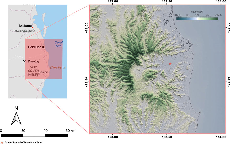
FIGURE 1. Maps of the studied region (Created using Natural Earth data in QGIS). Overview of the study site location in Australia and a zoomed in elevation map of the study site. y lat-min: ∼–28°, y lat-max: ∼–29°, x lon-min: ∼153.5°, and x lon-max: ∼153°.

FIGURE 2

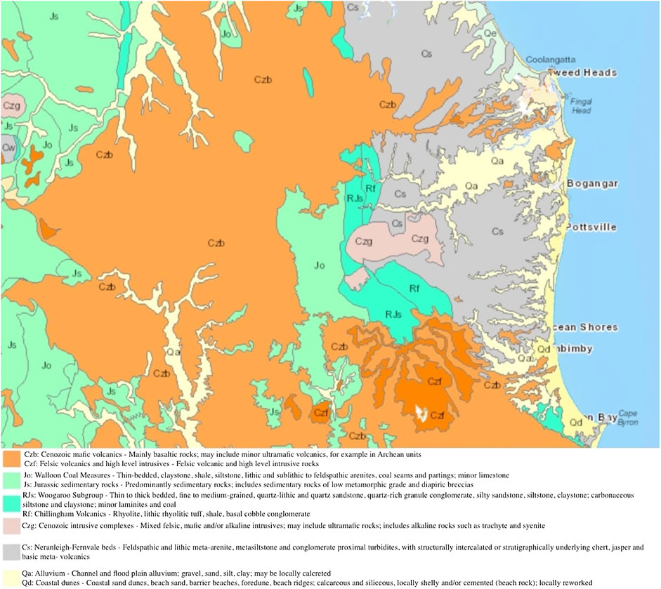
FIGURE 2. Geologic map of the studied area (Commonwealth of Australia, Geoscience Australia, 2020).

Materials and Methods

Model

A brief description of the Badlands LEM is provided here; for a more in-depth explanation of the model’s functionality readers are referred to Salles and Hardiman (2016) and Salles et al. (2018a). Badlands is a minimal numerical landscape and catchment model that efficiently solves erosion, sedimentation, diffusion, and flexure using a set of empirical and physical laws (Salles and Hardiman, 2016, p. 78). The associated equations do not differentiate between regolith and bedrock and assumes uniform substrate. The physics implemented by the model are simpler than the previously mentioned models (Coulthard et al., 2005; Hancock et al., 2010; Coulthard et al., 2012), but the purpose of Badlands is to take advantage of less complicated physics and provide an efficient code to model landscape dynamics at high resolution and over long temporal scales. An irregular mesh is implemented in order to prevent water flow directional bias. The continuity of mass is projected using the equation: ∂z/∂t = U − ∇⋅qs, in which z is elevation derived from the DEM, qs is the downhill soil flux (qs = qr + qd), ∇ ⋅ is a vector operator that controls spatial divergence and, for this study, U represents the tectonic conditions (assumed to be null in this study). Sediment transport is modeled using a stream power law that links topographic gradient to the flow accumulation:

$\text{qr}=-\text{κr }{\left(\text{qw}\right)}^{\text{m}}{(\nabla \text{z})}^{\text{n}}(1)$

where ∇z is the gradient in which sediment flux is oriented toward and qw is the rate of discharge (m²/yr). Hillslope transport processes are parameterized using the simple creep law:

${\text{q}}_{\text{d}}=-{\text{κ}}_{\text{d}}(\nabla \text{z})(2)$

where transport is reliant on local gradient and is scale-dependent.

For this study, the model required the inputs of topography in the form of a digital elevation model (DEM), bathymetric data, temporal evolution of annual precipitation rate (m/a), an annual SLR rate and an erodibility coefficient. The model then used these inputs to drive erosion, sedimentation, aggradation, transgression, river avulsion/incision, and the resulting landscape evolution of the simulated Tweed Caldera environment.

Experiments and Data

The digital topography and bathymetry of the Tweed Caldera drainage basin was derived from lidar (Royal Australian Navy, ∼50 m), multi-beam (Geoscience Australia and Australian Hydrographic Survey, ∼200 m), single-beam (Geoscience Australia and Australian Hydrographic Survey), satellite (Advanced Land Observing Satellite, 10 m; Shuttle Radar Topographic Mission, ∼30 m), and coastline data (Geoscience Australia, ∼10 m) provided by Australian federal and state government agencies in the form of DEMs and compiled by the eAtlas Three Dimensional Great Barrier Reef project (accessed April 2017) (Beaman, 2010). Badlands is able to model processes at high resolutions (10 m–2 km). The available elevation and bathymetric data for the drainage basin resulted in the DEM for the study at a resolution of ∼100 m. A model with 100 m resolution is sufficient to capture the regional changes in erosion and sedimentation. A higher resolution model would yield higher erosion and sedimentation rates, because with increasing DEM resolution, finer-scale tributaries of rivers and streams are included in the model, increasing the area subject to erosion and thus increasing the total sediment thickness over a given model run. This 100 m resolution DEM provides a minimum estimate for future increases in regional erosion and sedimentation. This exemplifies the need for government agencies to make high-resolution (>25 m) elevation and bathymetric data more readily available and easily obtainable. The data from the three dimensional Great Barrier Reef project is both spatially, in resolution and in coverage, a large improvement from the currently available data in the Australian Bathymetry and Topography grid (∼250 m) (Whiteway, 2009). As models continue to advance and develop more capabilities, elevation/bathymetric data resolution and availability will need to evolve simultaneously. This will allow for more comprehensive studies that can offer a greater understanding of landscape evolution processes met under climatic stress.

Realistic projections of precipitation and sea level rise were required as input for Badlands, in order to output practical responses of the landscape. The mean annual precipitation observed from 1972 to 2017 at the Murwillumbah observation point (Figure 1) was used as the baseline precipitation value for each model, beginning in 2020. This sight is set in between Tweed Heads and Mount Warning, and has a climate consistent with the humid subtropical climate of the catchment. The observed annual precipitation, using the baseline average from 1972 to 2017, was ∼1,600 mm per year. There are also regions of the caldera averaging much higher levels, like Nightcap National Park in the Southern region of the caldera which averages ∼2,300 mm annually (the highest in New South Wales), so a more pronounced erosional effect in these areas would be expected. Precipitation projection data was taken from “Climate Change in Australia” (climatechangeinaustralia.gov.au), in which data from a set of 50 current generation climate models for Australia were reviewed and given a confidence assessment (Clarke et al., 2011) (Table 1). It is noteworthy to mention that precipitation patterns in Australia are extremely difficult to project and relatively uncertain (CSIRO, 2015). While average rainfall is predicted to have no significant change for the Eastern region of Australia through the 21st century, the intensity and frequency of extreme rainfall events are projected to increase with temperature. The Queensland Government released a study that predicted a 5% increase in rainfall intensity per °C of mean temperature gain (Queensland Government, 2010). Moreover, the region’s average rainfall rate is approximately 1,000 mm more than the average for New South Wales. This relatively high amount of precipitation is predicted to increase as wet areas are projected to get wetter (Trenberth, 2011). Because the majority of models show little change in average precipitation patterns in northeastern New South Wales and the climate for the region is relatively wet, we will use the higher end of the projections in order to explore the effect of an increase in precipitation (+5%) for the most likely occurrence (–5% to +5%) by the end of the century. It is also important to note that this projection is for a region spanning the coastline from the study site (wetter climate) to Sydney (drier climate) and therefore, has significant potential for differences in projections due to orographic changes and coastal geometry (climatechangeinaustralia.gov.au). The average annual precipitation was incrementally increased every decade by ∼10 mm/a (0.625%) in order to see a 5% increase from baseline levels by the end of the century and kept at a constant rate past 2100.

TABLE 1

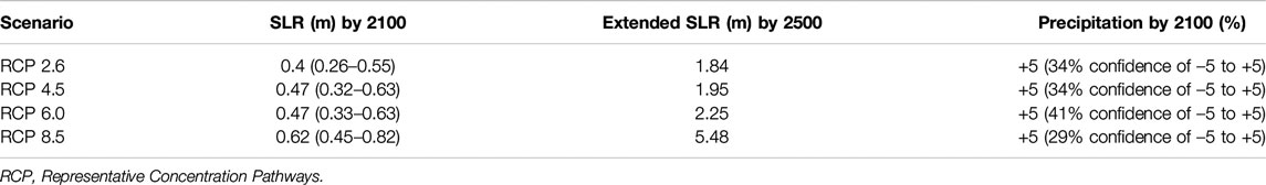
TABLE 1. Table showing sea level rise by 2100 (m), sea level rise (SLR) by 2500 as projected by the extended concentration pathways, and rates of increase in precipitation by 2100.

Regional northeastern New South Wales sea level rise projections for present-day to 2100 were derived from the Representative Concentration Pathways (RCP) relative to the average from 1988 to 2005 and are based on the 5–95% range of model results for SLR, but should only be considered likely (greater than 66% probability) (CSIRO and Bureau of Meteorology, 2015). Due to lack of regional SLR projection data past 2100, global extended SLR projections for 2100–2500, extracted from Jeyrejeya et al., (2012), were used (Table 1). Because there are many uncertainties attributed to scenarios past 2100, such as ice sheet response to climatic variation, long-term ocean heat uptake, and deep water formation (Jeyrejeya et al., 2012), it is important to note that these Extended Concentration Pathways (ECP) do not represent consistent scenarios, but are “what if” experiments that were derived using the basic principles of each RCP scenario and are produced for the purpose of having available data sets for longer-term research (Vaughn, 2008). It is also noteworthy to mention that the ECP scenarios do not take into account non-linearities such as the partial collapse of the West Antarctic Ice Sheet (WAIS), which would significantly raise global sea levels. We make use of the ECP scenarios in order to get a longer-term understanding of the potential mafic sediment supply has to sequester carbon on a regional scale. Silicate weathering is a long-term process, but enhanced silicate weathering is a concept that could effectively partially contribute to the mitigation of anthropogenic emissions. The inclusion of ECP scenarios, in order to project out to the year 2500, and the use of relatively lower resolution DEM data (>25 m), introduces uncertainties in the model results, swaying our model to more conservative estimates due to the lack of available relatively high resolution (<25 m) DEM data and causing for uncertain climate predictions the further we model into the future, but the overall pattern of mafic sediment being supplied to coastal erosive environments is expected to be fairly robust as the region experiences future shifts in climate.

A third variable that has significant control over the output of the model is the erodibility coefficient, which controls the magnitude of erosion at the surface of the simulated environment. In this study, the erodibility coefficient was set at 8e⁻⁵/yr and kept constant throughout all runs. The coefficient is dependent upon lithology, precipitation rate, channel width, channel hydraulics and flood frequency within the region. The value used in this study was determined due to the fact that the Tweed Caldera basin largely consists of volcanic basaltic rock and some minor sandstone, both of which are vulnerable to erosion; there are also rhyolite conglomerates that are demonstrated by the larger protruding rock formations (i.e., Egg Rock or Mount Doughboy), due to their higher resistance to weathering and the surrounding landscapes vulnerability to erosion (Solomon, 1964). The extreme slopes of the caldera, high precipitation rates, and vast network of river channels were also considered in choosing an appropriate erodibility coefficient.

In order to better understand how plausible future ice sheet melting can impact global sea levels and subsequently influence regional landscape dynamics, our study simulated three RCP scenarios (2.6, 4.5, and 8.5) with projected WAIS contributions. Plausible projections of WAIS evolution/collapse were derived from a study by DeConto and Pollard (2016), in which a newly improved numerical ice-sheet model, that implements model physics and parameter values previously used for simulations of past periods when the Antarctic Ice Sheet was melted to some degree. This model was used here to consider the effects of how Antarctica may evolve over the next five centuries. The global sea level rise values extrapolated from the ice-sheet model were added onto the three initial RCP/ECP projections. The values differ greatly from RCP 2.6 to RCP 8.5 due to the extreme sensitivities of ice sheets to warming, often referred to as “tipping points.” For example, in the modeled WAIS RCP 4.5 scenario, almost the entire ice sheet collapses by 2500, primarily because the retreat of Thwaites Glacier and subsequent retreat of the Aurora Basin into the deep WAIS interior; compared to a relatively minimal response of the ice sheet in the RCP 2.6 scenario, raising global sea levels by only 0.2 m by 2500 (DeConto and Pollard, 2016). In RCP 8.5, little effect is seen on ice by 2100 due to an increase in precipitation keeping most of the sheet stable, but by 2250 the entire WAIS collapses because of the extreme atmospheric warming and regional dynamics of Antarctica; eventually by 2500 retreat of ice into basins results in a AIS contribution of 12.3 m to global mean sea level rise (DeConto and Pollard, 2016).

For the purpose of understanding the influence local precipitation rates have on the dynamics of surrounding landscapes, specifically within the Tweed Caldera basin, four scenarios were created in which all variables, except annual average precipitation rates, are held constant. For scenario one, the precipitation values are the same as all the initial RCP model runs with a baseline precipitation value of ∼1.6 m/a and a 5% increase by 2100, followed by a constant rate of increase until 2500. Two more scenarios were run with the baseline precipitation value kept the same at ∼1.6 m/a, but a 10% and 15% increase by 2100 and the rate of increase kept constant until 2500. Our final precipitation scenario used the same baseline values as the previous scenarios, but a 5% decrease in annual precipitation by 2100 and a constant rate of decrease until 2500. This scenario was used to both compare the landscape impact of different plausible future precipitation scenarios and because many regions worldwide, including the chosen region, have uncertainty of how precipitation could change (Collins et al., 2013). For this reason, an understanding of the impacts of both an increase and decrease in regional precipitation rates needs to be better understood.

Results

Representative Concentration Pathway Scenarios

Model outputs from each scenario differed (at times significantly) based on the imposed climatic changes, the main controlling factor being the rate of sea level rise. Impacts to the upland catchment area are more extreme both in magnitude and rate for the scenarios with greater climatic change (i.e. RCPs 4.5–8.5 and AIS 4.5–8.5). For example, when rates of SLR were high, impacts to the local dynamics and landscape, such as infill of inland bodies of water, river avulsions and upstream flooding, occurred much more quickly and to a greater extent than scenarios with lesser rates of SLR, showing relatively small basin changes.

With very few climatic variations under RCP 2.6, compared to the rest of the scenarios, landscape response was modest as expected. The main impacts to upstream catchment observed in the model output were effects to the drainage network (i.e., main channels and tributaries). These effects occurred in the form of river avulsions and slight infill of inland bodies of water and bays. All of these impacts were due to the changing rates of erosion and deposition caused by the variation in local climate. Analysis of the model output allows for a quantification of the total deposited sedimenlt volume within the floodplain (25.2 million m²). We were able to measure the supplied sediment by defining a polygon that contained the floodplain region and analyzing the defined area’s sedimentation using a Badlands companion Jupyter notebook (https://github.com/badlands-model). We also estimated the sediment volume uncertainties by calculating the standard deviation of the supplied sediment for all scenarios by 2100 and 2500. Using this calculation (±) gives us an estimated standard margin of error for each scenario’s supplied sediment volume estimate, and provides a more thorough understanding of the potential for mafic sediment’s to be supplied to erosive environments within the catchment. By 2100 a total of ∼30 ± ∼1.4 million m³ is deposited and by the end of the model run ∼106.5 ± ∼32 million m³ of mafic sediment is deposited into erosive environments, with an average deposited sediment thickness of ∼4 m. The increase in sea level for RCP 2.6 was so small that no significant impact can be observed.

Comparatively, impacts under RCP 4.5 and 6.0 do not differ significantly by 2100, but by 2500 there is a noticeable contrast between the two landscapes (Figures 3 and 4). Under RCP 6.0 the floodplain experiences a greater increase in deposition compared to RCP 4.5, and in turn less sediment is discharged into the marine environment. By 2100–30 ± ∼1.4 million m³ of sediment is deposited into the floodplain for both scenarios, but by 2500 only ∼96 ± ∼32 million m³ is deposited under RCP 4.5, whereas a much more significant amount of ∼172.5 ± ∼32 million m³ occurs within the floodplain under RCP 6.0, resulting in an average thickness of ∼3.8 and 6.5 m, respectively. Although sea level rise is relatively insignificant throughout the RCP 4.5 scenario, the slightly higher magnitude of sea level rise under RCP 6.0 causes a significant difference in landscape dynamics. The increase in SLR forces extra sediment to be deposited in upstream environments where there is a high potential for an enhanced silicate weathering affect to occur.

FIGURE 3

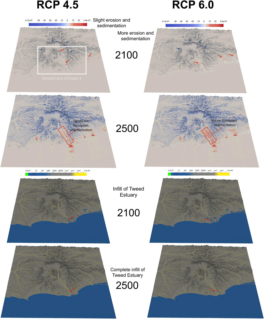
FIGURE 3. Comparison of (Representative Concentration Pathways) RCP 4.5 and RCP 6.0. Visualizations of erosion/deposition with red regions indicating areas of deposition and blue regions indicating areas of erosion (m²/a) (top). Visualizations of discharge with brighter yellow colors indicating greater discharge rates (m²/a) (bottom), with varying impacts between scenarios and over time.

FIGURE 4

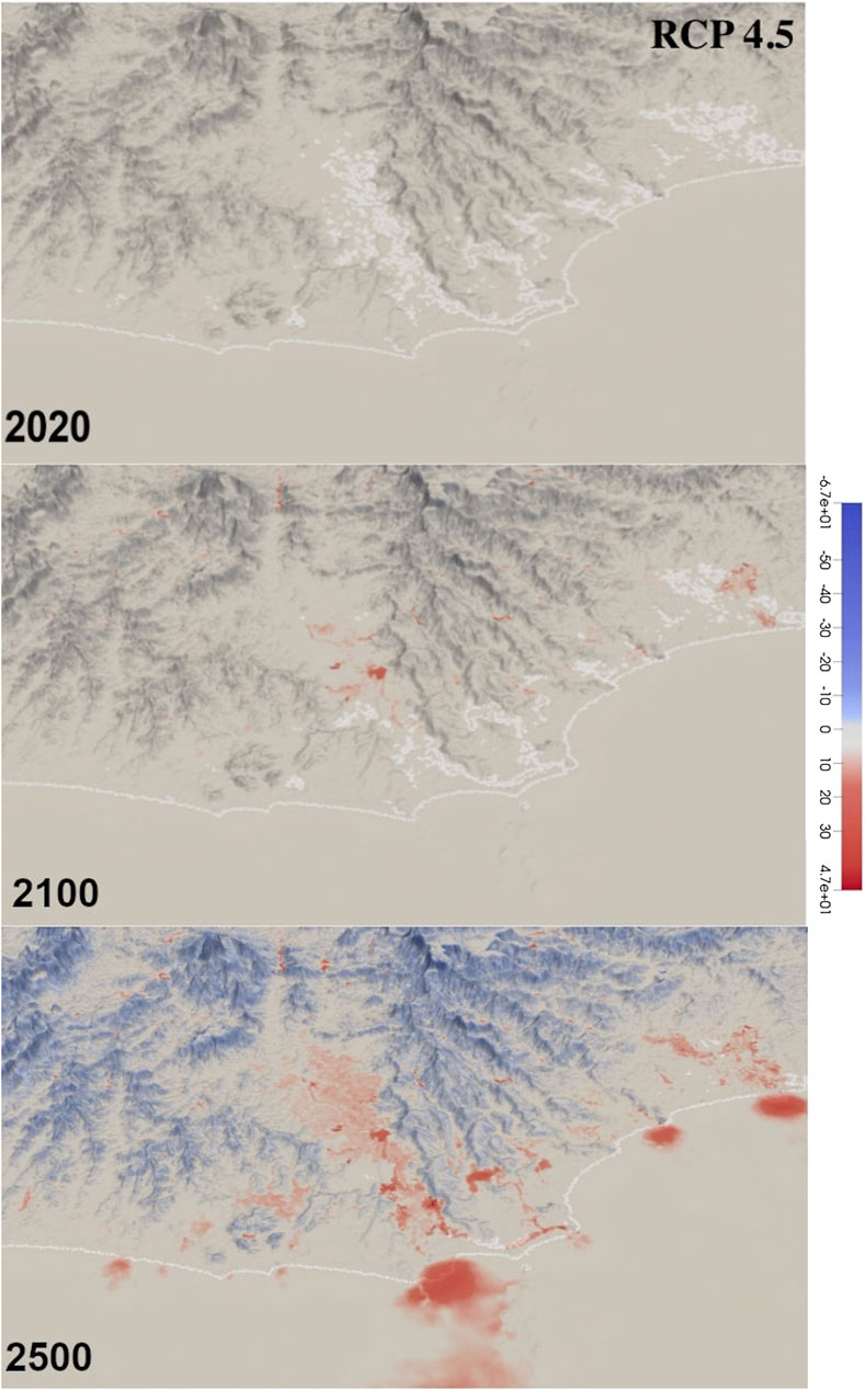
FIGURE 4. Zoomed in regional visualization of the Tweed Valley floodplain region under Representative Concentration Pathways 4.5, illustrating the deposition of mafic sediment supply into erosive environments, and demonstrating the impact of sediment supply on local dynamics. Red areas indicate deposition and blue areas indicate erosion (m²/a).

Due to significant variation of local climate in the RCP 8.5 scenario, the consequential impacts to landscape dynamics are accentuated compared to the previous scenarios (Figures 5 and 6). Under this “business as usual” scenario, sea level rise plays a huge role in landscape dynamics. Significant amounts of sediment are deposited into the ocean through mainstreams, but once SLR becomes significant enough, marine deposition stops. This forces large amounts of sedimentation inland, near coastal areas and within the floodplain, where weathering will occur. During the first century, sedimentation of the floodplain occurs at a slightly faster rate than the previous scenarios and a total of ∼32 ± ∼1.4 million m³ of sediment is deposited. Once SLR becomes dramatic enough to control the regional dynamic impact, there is a slowing of the deposition within the floodplain, in which ∼107 ± ∼32 million m³ are deposited by 2500, and an increase of deposition in other areas of the studied region (i.e. the deposition is pushed north and south along the coast). This deposition within the floodplain results in an average thickness of deposited sediment of ∼4 m. Eventually, inundation due to dramatic SLR is the main climatic forcing controlling inland dynamic response.

FIGURE 5

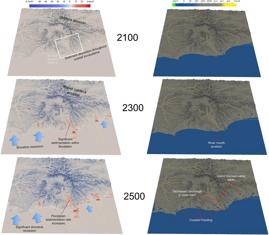
FIGURE 5. Visualizations of Representative Concentration Pathways 8.5 erosion and deposition, with red regions indicating areas of deposition and blue regions indicating areas of erosion (m²/a) (left). Visualizations of discharge with brighter yellow colors indicating greater discharge rates (m²/a) (right) demonstrating dynamic differences between 2100, 2300, and 2500.

FIGURE 6

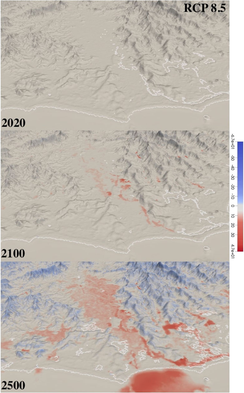
FIGURE 6. Zoomed in regional visualization of the Tweed Valley floodplain region under Representative Concentration Pathways 8.5, illustrating the deposition of mafic sediment supply into erosive environments and the heavy accumulation over time, as well as the the impact of sediment supply on local dynamics. Red areas indicate deposition and blue areas indicate erosion (m²/a).

Antarctic Ice Sheet Scenarios

Under RCP 2.6 and 4.5, DeConto and Pollard projected minor contributions from the Antarctic Ice Sheet to global sea level rise (2016). Model output shows a similar landscape reaction to RCPs 2.6 and 4.5 under this scenario, with an accentuated impact under RCP 4.5 toward the end of the model run, due to a tipping point not being hit within the ice sheet. Deposition within the floodplain remains similar to those scenarios as well, with ∼30 ± ∼1.4 million m³ deposited within the floodplain by 2100 under both scenarios and ∼115 and ∼163 ± ∼32 million m³ by 2500, respectively, resulting in an average thickness of ∼4.5 and ∼6 m. Conversely, under RCP 8.5 a tipping point is hit early in the scenario and the AIS contributes significantly to global sea level rise (DeConto and Pollard, 2016) (Figures 7 and 8). In response, the dynamics and landscape of the modeled basin are heavily impacted with new dynamical responses being observed as SLR hits a certain threshold. For the first few centuries (2020–2200) basin impacts are relatively similar to those seen under RCP 8.5, illustrated by the deposition of ∼27 ± ∼1.4 million m³ of sediment within the floodplain by 2100. Eventually, the tipping point hit in the AIS causes extreme amounts of SLR and this forces all deposition upstream, resulting in ∼315 ± ∼68 million m³ of deposition within the floodplain by 2500 and an average thickness of ∼11.5 m, as well as inundating the entire coastline. This increase in floodplain sedimentation causes a large rise in elevation within the area by the end of the simulation. Other than forcing changes in elevation, sedimentation is not sufficient to fill the accommodation space formed by extreme rates of SLR. This scenario would scatter a significant amount of newly eroded/deposited olivine within environments in which weathering could occur for a sustained period of time.

FIGURE 7

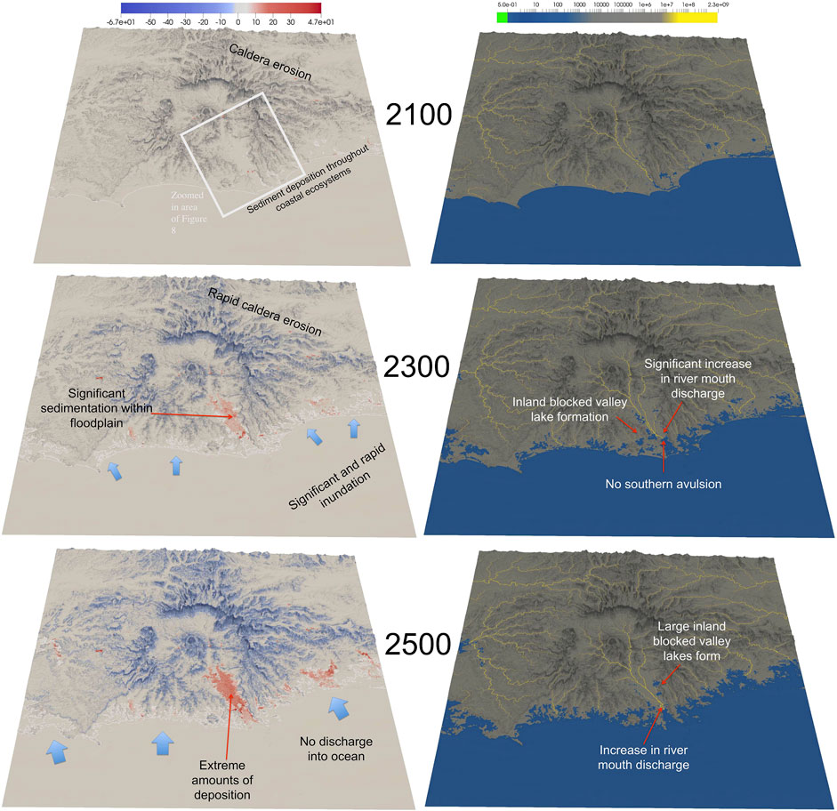
FIGURE 7. Visualizations of Representative Concentration Pathways 8.5 Antarctic Ice Sheet erosion and deposition, with red regions indicating areas of deposition and blue regions indicating areas of erosion (m²/a) (left). Visualizations of discharge with brighter yellow colors indicating greater discharge rates (m²/a) (right) demonstrating dynamic differences between 2100, 2300 and 2500.

FIGURE 8

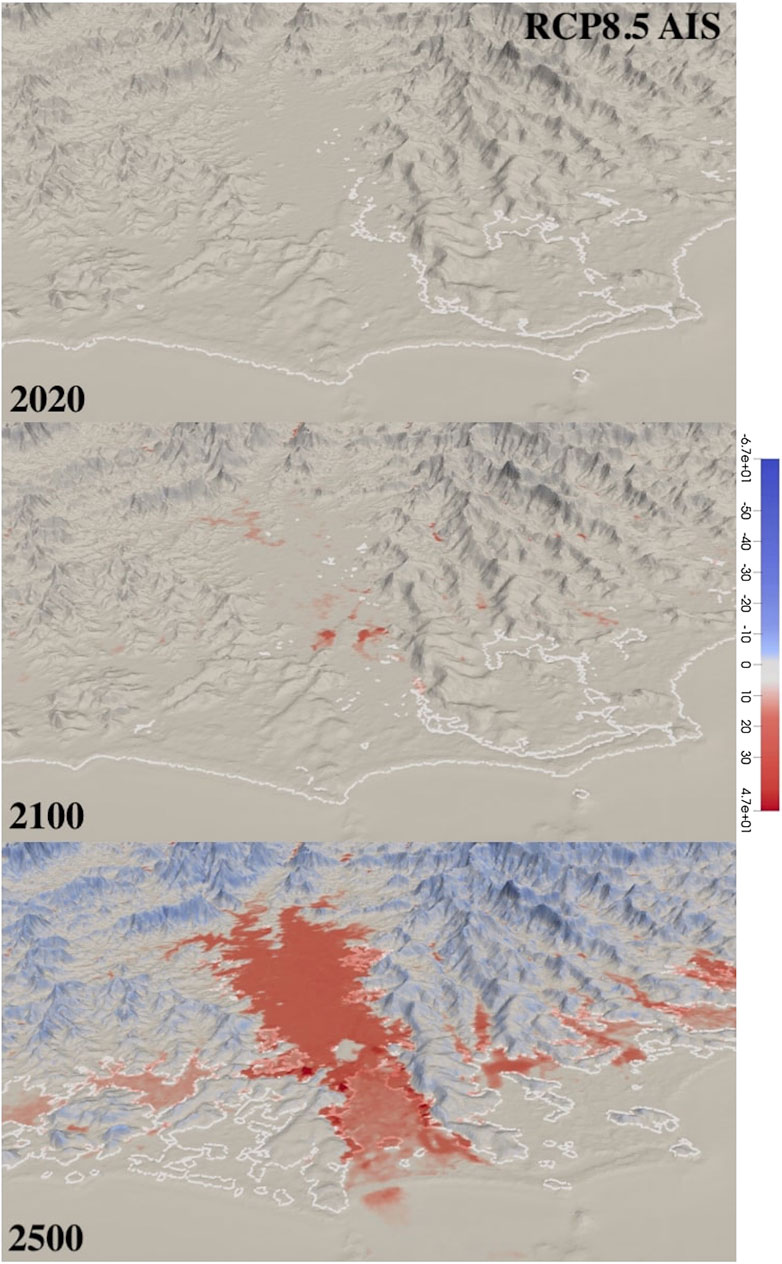
FIGURE 8. Zoomed in regional visualization of the Tweed Valley floodplain region under Representative Concentration Pathways 8.5 Antarctic Ice Sheet, illustrating the deposition of mafic sediment supply into erosive environments and the heavy accumulation over time, as well as the the impact of sediment supply on local dynamics. Red areas indicate deposition and blue areas indicate erosion (m²/a).

Under the RCP 8.5 scenario, the Antarctic Ice Sheet is projected to contribute a considerably large amount to global sea levels (DeConto and Pollard, 2016). Model output shows dramatic impacts to the local landscape, specifically the floodplain in which most of the eroded material is deposited, as a consequence of the high rates of sea level rise (Figure 9). There is seemingly also a change in local dynamics caused by the extreme magnitude and rate of environmental change forced by the AIS. Rates of sea level rise are high, evidenced by the fact that no sediment ever gets deposited to the original shoreline/marine environment, and is instead all being deposited within the floodplain/upstream. This results in a rise in elevation of the landscape by ∼20 m in some areas of the floodplain. Inundation is so significant that the coastline is no longer recognizable within the first few centuries. Throughout the entire scenario, rates of SLR are solely the forcing that controls deposition and basin changes. It is important to remember that these AIS model runs are “what if” scenarios and not likely or projected to actually occur. These scenarios can help create a better understanding of the massive potential ice sheets hold in completely altering worldwide landscapes/dynamics, and the control sea level rise has on sedimentation processes within a region.

FIGURE 9

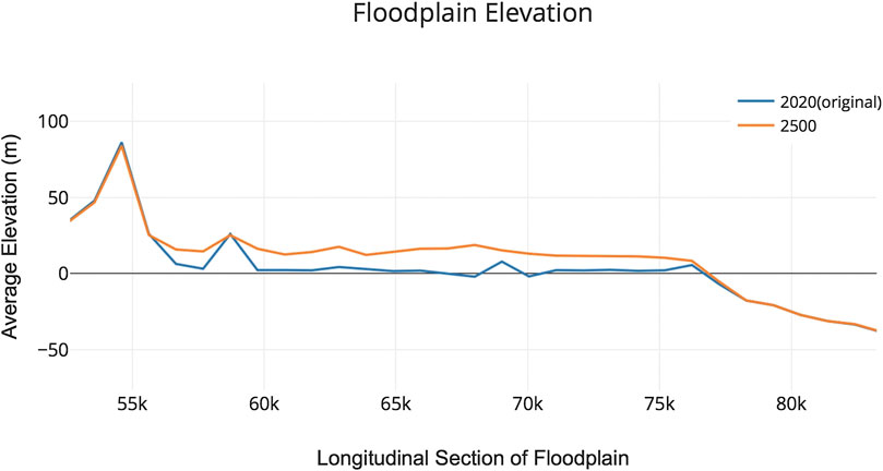
FIGURE 9. Comparisons of floodplain elevation between 2020 and 2500.

Precipitation Scenarios

For each precipitation scenario, model output shows relatively similar variations in local landscape dynamics, but with difference in magnitudes of change. Under the first precipitation scenario, the same 5% increase in precipitation by 2100 is used, but sea levels are held constant. Model output shows a noticeably different impact when there is no variation in sea level. Sediments are discharged into the ocean, miniscule amounts of inland deposition occur, evidenced by a total deposition within the floodplain of ∼28.5 ± ∼1.4 million m³ by 2100 and ∼78 ± ∼32 million m³ and an average thickness of ∼3 m by 2500. Consequently there is very little infill of inland bodies of water, but the southern avulsion of the mainstream stem still occurs (Figure 10). When the basin was put under a stress of both a 10% and 15% increase to the rate of precipitation by 2100, the impacts were very similar to the previous precipitation scenario in which the majority of basin impacts were seen within the floodplain and marine environments into which sediments are being discharged (Figure 11). By 2100–30 ± ∼1.4 million m³ of mafic sediment are supplied to the floodplain for both scenarios, and by 2500 a total of ∼82 million m³ and ∼88 m³ ± ∼32 million m³ are deposited respectively, resulting in an average thickness of ∼3.25 and ∼3.5 m. A 5% decrease in precipitation shows no significant changes in landscape or dynamics and has a similar response as RCP 2.6.

FIGURE 10

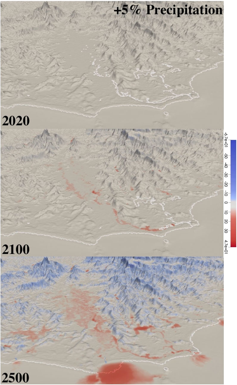
FIGURE 10. Zoomed in regional visualization of the Tweed Valley floodplain region under a 5% increase in precipitation, demonstrating the significant control sea level rise has on the regional transport of mafic sediment. Red areas indicate deposition and blue areas indicate erosion (m²/a).

FIGURE 11

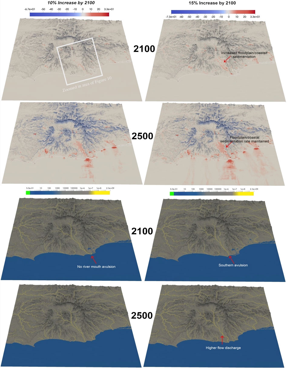
FIGURE 11. Comparison of precipitation scenarios: +10% (left) and +15% (right). Visualizations of erosion/deposition with red areas indicating deposition and blue areas indicating erosion (m²/a) (top) and visualizations of discharge with brighter yellow colors indicating greater discharge rates (m²/a) (bottom), illustrating the erosional, depositional and landscape dynamics from 2100–2500.

These precipitation scenarios illustrate the influence sea level rise has on the landscape dynamics of this region. Comparatively, when holding sea levels constant the effect seen to the regional sedimentation, landscape, and dynamics is significantly smaller. Even with large increases in precipitation (10–15%) and subsequent increases in local erosion, the depositional and landscape response were still relatively small. Although the erosion rates increase, most of the newly eroded sediment are fully transported through the river systems and deposited into the ocean. Some sediment is deposited within the floodplain, but not enough to cause significant inland impacts or any significant accumulation until much later in the scenarios. These scenarios effectively demonstrate the interplay of regional sea level rise and inland landscape dynamics.

Scenario Comparison

A qualitative analysis of the model output demonstrates some clear differences in the impacts to the landscape between each climatic scenario. It is also clear that the majority of the effects occur within the floodplain of the caldera, where the Tweed River transports/deposits sediment. This is an energetic and ideal environment for weathering and subsequent carbon sequestration to occur. In order to better understand these affects, the impacts of each scenario to elevation (caused by the amount of sediment deposited) and discharge within the floodplain was analyzed, as well as a comparison of these impacts between all the different climatic scenarios (Figure 12).

FIGURE 12

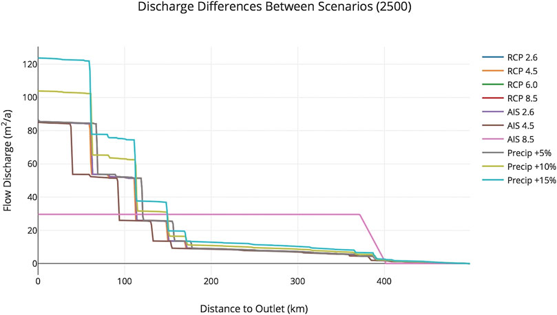
FIGURE 12. Comparison of discharge rates within the Tweed River by 2500 between all climatic scenarios.

FIGURE 13

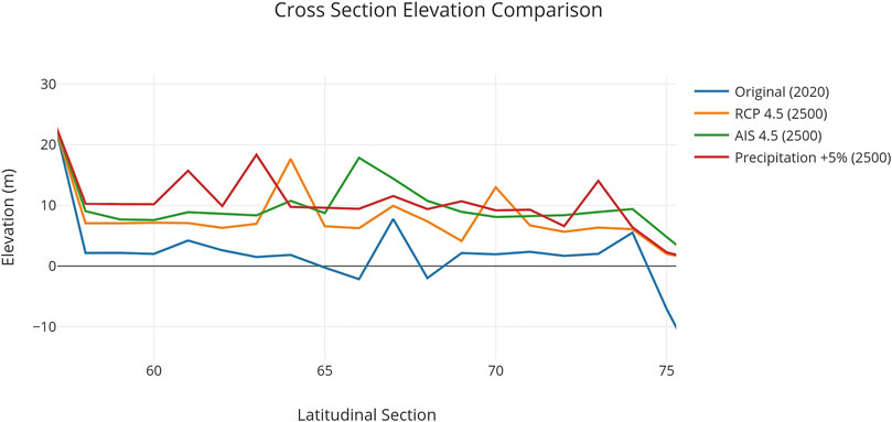
FIGURE 13. Comparison of the elevation differences between a few scenarios in a cross section of the floodplain region (by 2500), demonstrating the drastic control future climate change scenarios.

Analyzing the differences between scenarios of discharge within the Tweed River by 2500 not only shows that climatic factors varyingly impact the dynamics within the region, but also demonstrates how transport of eroded sediment can change depending on the climatic influences at play. Under extreme scenarios like AIS 8.5, there are subsequent extreme impacts and the vast majority of sediment is trapped within the inland environments. Under more mild scenarios like RCPs 2.6, 4.5 and 6.0, the impacts are relatively consistent and much less extreme, but a significant amount of sediment is still deposited within the coastal and floodplain environments. The precipitation scenarios show a large increase in discharge throughout the stream due to no other climatic influences forcing a decrease and pushing sediment further inland. Even when precipitation rates are identical between the initial precipitation scenario and all the RCP/AIS scenarios, there is still a greater increase in discharge of the mainstream when sea level rise is not a factor.

Analyzing the comparison of impacts to elevation (deposition) illustrates the differences in the accumulation of sediments in weatherable environments between each scenario. Figure thirteen shows the greatest impact is experienced in the floodplain, where elevation is increased in all scenarios (compared to 2020 levels), and to a lesser degree in areas of high relief where a decrease in elevation is seen due to erosion. This figure better quantifies the ability of the regional environment to erode, transport, and deposit the mafic sediment.

Performing a quantitative analysis of the deposition occurring within the floodplain allows for a more precise comparison between different climatic scenarios and illustrates the major controls of sedimentation within the region (Figure 14). By 2100, there is a similar response of floodplain deposition under all scenarios, with the sum of deposited sediment volume around ∼30 ± ∼3 million m³. Significantly different regional responses are experienced under RCP 6.0 and RCP 8.5 AIS after 2100, as well as RCP 4.5 AIS after 2300. Under RCP 6.0, there is a large increase in the rate of floodplain deposition between 2100 and 2300, but that rate significantly slows after 2300. Whereas in RCP 8.5 AIS, there is a similar large increase in the rate of floodplain deposition by 2100, but that rate never plateaus. All other scenarios show similar responses, in which there is a relatively linear increase in floodplain deposition until 2500, where the sum volume of sedimentation reaches ∼100 million m³. These responses demonstrate the non-linear control that sea level rise has on regional sedimentation processes. Under RCP 6.0, the sea level rate is high enough to force sediment up stream and slow marine deposition, but low enough that deposition is not forced into other coastal regions to the north and south of the floodplain. Under RCP 8.5 AIS, SLR is so extreme that all sedimentation is forced directly inland of where the sediment is being transported (the Tweed River) and cannot be deposited into marine environments or be transported north or south along the coast.

FIGURE 14

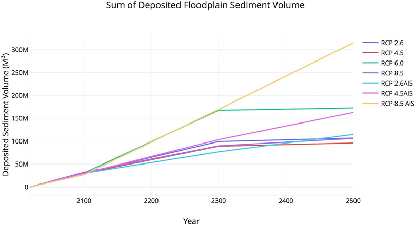
FIGURE 14. Comparison of the sum volume of deposited sediment within the floodplain under all scenarios (not including precipitation scenarios).

Along with a quantification of the modeled sediment volume supplied to the erosive environments, a further assessment of the consequent impact to enhanced silicate weathering will help visualize the overall enhanced sequestering potential of volcanic landscapes. According to the model results and regional geologic map (Figure 2), the area in which erosion is occurring consists almost entirely of mafic and ultramafic basalts. Based on this regional geologic composition and a USGS figure quantifying the general composition of basalts (Stoffer, 2002), we conservatively generalize the percentage of the supplied sediment volume’s mineral composition to consist of 25% olivine. The mean supplied sediment volume of the most likely future scenarios (RCP 2.6, 4.5, 6.0, and 8.5) by 2100 is ∼30.5 million m³ ± ∼92,500 m³, and by 2500 is ∼120 ± ∼30 million m³. The subsequent average volume of eroded olivine that is transported to erosive environments is ∼7.6 ± ∼250,000 m³ by 2100 and ∼30 ± ∼8.8 million m³. According to Schuiling (2017), the weathering rate of olivine grains in a natural wet environment, like the Tweed floodplains, would be approximately 50 microns per year. Taking our estimate of total volume of mafic and ultramafic rock eroded and using the CO₂ sequestration estimate of 0.80–1.10 tons of CO₂ sequestered per ton of rock eroded from Moosdorf et al. (2014), according to our model results under the most likely future climate scenarios in the Tweed catchment we estimate a total sequestration of ∼52–73 million tons of CO₂ by 2100 and ∼206–284 million tons by 2500. This relative amount of sequestered CO₂ from naturally enhanced silicate weathering could be expected in other similar volcanic landscapes, and could cumulatively amount to a significant impact, thus it is imperative to start studying this effect in more detail and in other landscapes.

Conclusions/Discussion

Based on the differences between the model output of varying scenarios, it can be concluded that climate change may significantly influence local erosion, deposition, and landscape evolution on a drainage basin scale in a volcanic landscape. Our models pinpoint particular regions where climate change can create environments in which enhanced natural carbon sequestration may occur due to increased mafic sediment supply to weathering inducive environments, as well as demonstrating what factors are having the most influence on this negative feedback loop and regional basin evolution. This mafic transport and supply is evidenced by the relatively small basin-wide elevation change seen in all scenarios by 2500 due to enhanced erosion and deposition, with a prominent decrease in the caldera areas with high relief and increase in areas within the Tweed Valley floodplain where sediments are being deposited (Figure 8). This impact on local elevation is related to the amount of sediment being eroded in each scenario and is therefore partially controlled by the changing precipitation rates, but as shown by the model output, is highly controlled by the rate of SLR. The rate and magnitude of SLR is the dominant control of where, when, and how much sediment is deposited within the region. Once SLR reaches a certain threshold, sediment within the mainstream, and other important sediment transporting streams, begins being deposited upstream throughout the floodplain rather than entering the marine environment. This phenomenon can be observed with a SLR rate equal to and greater than that seen in RCP/ECP 4.5, but is absent in scenarios with lower or stable SLR rates. This reflects the control of accommodation on deposition and the impact that sea-level change has on accommodation space. With a rise in local relative sea level, accommodation is simultaneously affected in a way that forces sediment to accumulate upstream within the energetic river channels that are transporting sediment, as well as in the overbank areas. These areas are effective environments for weathering to occur. Since the Tweed River is a mature stream, it has developed an equilibrium profile in which erosion is occurring in the upper tracts of the stream with sediments subsequently being deposited in the marine environment. Once climate change is drastic enough to significantly impact stream dynamics via increased sediment loads and/or changes in accommodation, then the profile is disturbed and moved out of equilibrium. This is seen in the majority of model runs, with the exception of the precipitation scenarios. This reinforces the idea that local dynamics, especially sedimentation, within the Tweed basin are heavily influenced by sea-level change and are sensitive to shifts in climate. Model results are only projections, and reality is more complex than what can be captured within any model, but our study using Badlands is useful to better understand the first-order mechanisms played by surface processes in potentially enhancing silicate weathering.

Some model scenarios show that although the overall shoreline pattern is a transgression, there can be regression at the mouths of rivers. This means that although SLR should be forcing a retreat of shorelines, there are some scenarios in which this effect can be overpowered by the amount of sediment being eroded/transported. This effect is only seen in RCPs 4.5 and 6.0 in which SLR is moderate enough and erosion is significant enough to allow for shoreline transgression, with shoreline regression occurring only at select river mouths where the sediment load is large enough to allow for growth. Under these circumstances, sediments are transported to coastal environments that are dominated by wave action. These scenarios would further allow for enhanced silicate weathering to occur. Future studies in this region may improve our understanding of the weathering rate of olivine in marine environments.

The ice sheet scenarios projected by DeConto and Pollard applied within the model runs vary greatly from the original RCP scenarios (except RCP 2.6) (DeConto and Pollard, 2016). This has to do with tipping points being reached within the ice sheet due to warming, followed by rapid impacts to the AIS and global sea levels. However, tipping points within ice sheets are a relatively ill constrained. Model projections from this study are a good example of why tipping points within ice sheets need to be better understood. Under AIS scenario 2.6 very miniscule impacts are observed, but under AIS scenarios 4.5 and 8.5 the impacts to the basin landscape are extreme. In such extreme SLR scenarios, all catchment response to the changing climate is essentially overpowered by the significant inundation that occurs by 2500. In scenarios in which sea level is significant enough, but not overpowering (RCP 8.5), or in the extreme SLR scenarios, but before the inundation effect is too overpowering, the formation of inland blocked-valley lakes can be observed. This is caused by the previously mentioned accommodation effect pushing deposition upstream. As the increased sediment load, caused by the increased erosion, is deposited upstream and not within the ocean, aggradation starts occurring. Many of the smaller tributaries of the mainstream, or some of the larger streams in the catchment, are unable to aggrade at the same rate as those larger streams. This essentially creates a natural dam and floods the smaller tributaries, effectively creating the inland blocked-valley lakes. The formation of these lakes would have major ecological and socioeconomic impacts as they would form within developed floodplains, and could create environments in which weathering would not be as effective. Under such extreme scenarios, SLR would be so extreme that much of the weathering potential in high-energy fluvial/floodplain environments may decrease.

Another impact that is consistently seen throughout all model scenarios is changes in discharge at the mouth of the mainstream over time and between scenarios. This impact is most noticeable within the mainstream (Tweed River) and throughout the floodplain. This is most likely due to the increased sediment load over time and between scenarios. Increased sediment within streams, due to increased precipitation as well as sea level/accommodation forcing, results in variations in river discharge and downstream incision. Furthermore, channel shape changes as the riverbeds aggrade and streams avulse, contributing to the changes in discharge. This could potentially impact the effectiveness of weathering within streams and force deposition to occur in other environments.

In general, the model output shows that when the Tweed Caldera basin experiences a warming climate, the subsequent impacts effect erosion, deposition, discharge, elevation, relief and the overall evolution the local landscape/dynamics (hydromorphic and geomorphic). Specific landscape effects due to climatic changes are unique to each scenario and can differ greatly. As predictions and models become more precise and representative of realistic landscape dynamics, more future studies will need to be oriented toward smaller-scale, regional areas, and regional climate change. This will allow for a better understanding of the local dynamics and how they interact with environmental change. The information landscape models such as Badlands can provide will be valuable for informing future policies on how to best adapt to the regional and local effects of future climate change and how effective an environment could be as a carbon sink. Global weatherability and weathering has been one of the primary, if not the foremost, driver of Earth’s climate state (Macdonald et al., 2019). Artificially enhancing weatherability globally could be a viable mitigation strategy to anthropogenic carbon emissions. In order to pursue artificially enhancing olivine weathering as a potential mitigation action, the impact of increased olivine supply into coastal depositional systems and the rate of olivine weathering in different environments needs to be further investigated (Meysman and Montserrat, 2017). Our study has identified a region in which these questions could be addressed through additional experiments, observations, and models.

Data Availability Statement

Publicly available datasets were analyzed in this study. This data can be found here: ftp.earthbyte.org. Further inquiries can be directed to the corresponding author/s.

Author Contributions

Conceptualization: KM, TS, RM; Methodology: TS, KM, RM; Software: TS; Formal Analysis: KM; Investigation: KM; Resources: TS, RM; Writing-Original Draft: KM; Review and Editing: KM, TS, RM; Visualization: KM.

Conflict of Interest

The authors declare that the research was conducted in the absence of any commercial or financial relationships that could be construed as a potential conflict of interest.

Acknowledgments

We thank Jen Kay, Jai Syvitski and Dale Miller for their roles on this project as thesis committee advisors. This work was initially conducted as a month long independent study project at the University of Sydney and progressed into a Senior Bachelor Honor’s Degree Thesis at the University of Colorado Boulder (Manley, 2018).

References

Australia Department of Climate Change (2009). Climate change risks to Australia’s coast: a first pass national assessment. (Canberra): Australia Dept. of Climate Change.

Google Scholar

Beaman, R. J. (2010). Project 3DGBR: a high-resolution depth model for the Great barrier reef and coral sea. marine and tropical sciences research facility (MTSRF) project 2.5 i. 1a final report, MTSRF, cairns, Australia, 12 plus appendix 1. Plus Appendix. 1, 12.

Google Scholar

Blum, M. D., and Törnqvist, T. E. (2000). Fluvial responses to climate and sea‐level change: a review and look forward. Sedimentology 47 (s1), 2–48. doi:10.1046/j.1365-3091.2000.00008.x

CrossRef Full Text | Google Scholar

Braun, J., and Willett, S. D. (2013). A very efficient O (n), implicit and parallel method to solve the stream power equation governing fluvial incision and landscape evolution. Geomorphology 180, 170–179. doi:10.1016/j.geomorph.2012.10.008

CrossRef Full Text | Google Scholar

Bull, W. B. (1991). Geomorphic responses to climatic change. Oxford: Oxford University Press.

Google Scholar

Church, J. A., Clark, P. U., Cazenave, A., Gregory, J. M., Jevrejeva, S., Levermann, A., et al. (2013). Sea level change. Cambridge, England: PM Cambridge University Press.

Google Scholar

Clarke, J. M., Whetton, P. H., and Hennessy, K. J. (2011b). “Providing application-specific climate projections datasets: CSIRO's climate futures framework,” in MODSIM2011, 19th international congress on modelling and simulation. Editors F. Chan, D. Marinova, and R. S. Anderssen, (Perth, Western Australia: Modelling and Simulation Society of Australia and New Zealand).

Google Scholar

Coulthard, T. J. (2001). Landscape evolution models: a software review. Hydrol. Process. 15 (1), 165–173. doi:10.1002/hyp.426

CrossRef Full Text | Google Scholar

Coulthard, T. J., Hancock, G. R., and Lowry, J. B. (2012). Modelling soil erosion with a downscaled landscape evolution model. Earth Surf. Process. Landforms. 37 (10), 1046–1055. doi:10.1002/esp.3226

CrossRef Full Text | Google Scholar

Coulthard, T. J., Kirkby, M. J., and Macklin, M. G. (2000). Modelling geomorphic response to environmental change in an upland catchment. Hydrol. Process. 14 (11‐12), 2031–2045. doi:10.1002/1099-1085(20000815/30)14:11/12<2031::aid-hyp53>3.0.co;2-g

CrossRef Full Text | Google Scholar

Coulthard, T. J., Lewin, J., and Macklin, M. G. (2005). Modelling differential catchment response to environmental change. Geomorphology 69 (1), 222–241. doi:10.1016/j.geomorph.2005.01.008

CrossRef Full Text | Google Scholar

Coulthard, T. J., Macklin, M. G., and Kirkby, M. J. (2002). A cellular model of Holocene upland river basin and alluvial fan evolution. Earth Surf. Process. Landforms. 27 (3), 269–288. doi:10.1002/esp.318

CrossRef Full Text | Google Scholar

Couture, N. J., and Pollard, W. H. (2007). Modelling geomorphic response to climatic change. Clim. Change. 85 (3), 407–431. doi:10.1007/s10584-007-9309-5

CrossRef Full Text | Google Scholar

CSIRO and Bureau of Meteorology (2015). Climate change in Australia information for Australia’s natural resource management regions: technical report. Australia: CSIRO and Bureau of Meteorology.

Google Scholar

de Caritat, P., and Cooper, M. (2009). Preliminary Soil pH map of Australia. Record 2010. Geoscience Australia, Canberra. http://pid.geoscience.gov.au/dataset/ga/70105.

Google Scholar

DeConto, R. M., and Pollard, D. (2016). Contribution of Antarctica to past and future sea-level rise. Nature 531 (7596), 591–597. doi:10.1038/nature17145

CrossRef Full Text | Google Scholar

Dorn, R. I. (1994). “The role of climatic change in alluvial fan development,” in Geomorphology of desert environments (Netherlands: Springer Netherlands), 593–615.

Google Scholar

Dorn, R. I., DeNiro, M. J., and Ajie, H. O. (1987). Isotopic evidence for climatic influence on alluvial-fan development in Death Valley, California. Geology 15 (2), 108–110. doi:10.1130/0091-7613(1987)15<108:iefcio>2.0.co;2

CrossRef Full Text | Google Scholar

Eisenhauer, A., Zhu, Z. R., Collins, L. B., Wyrwoll, K. H., and Eichstätter, R. (1996). The Last Interglacial sea level change: new evidence from the Abrolhos islands, West Australia. Geol. Rundsch. 85 (3), 606–614. doi:10.1007/bf02369014

CrossRef Full Text | Google Scholar

Hancock, G. R., Lowry, J. B. C., Coulthard, T. J., Evans, K. G., and Moliere, D. R. (2010). A catchment scale evaluation of the SIBERIA and CAESAR landscape evolution models. Earth Surf. Process. Landforms. 35 (8), 863–875. doi:10.1002/esp.1863

CrossRef Full Text | Google Scholar

Hancock, G. R., Willgoose, G. R., and Evans, K. G. (2002). Testing of the SIBERIA landscape evolution model using the Tin Camp Creek, Northern Territory, Australia, field catchment. Earth Surf. Process. Landforms. 27 (2), 125–143. doi:10.1002/esp.304

CrossRef Full Text | Google Scholar

IPCC (2001). Climate change 2001: the scientific basis. Editors J. T. Houghton, Y. Ding, D. J. Griggs, M. Noguer, P. J. Van Der Linden and D. Xioaosu, Contribution of working group I to the third assessment report of the intergovernmental panel on climate change Cambridge: Cambridge University Press, 944.

Google Scholar

Jevrejeva, S., Moore, J. C., and Grinsted, A. (2012). Sea level projections to AD2500 with a new generation of climate change scenarios. Glob. Planet. Change 80, 14–20

Google Scholar

Knox, J. C. (1972). Valley alluviation in southwestern Wisconsin. Ann. Assoc. Am. Geogr. 62 (3), 401–410. doi:10.1111/j.1467-8306.1972.tb00872.x

CrossRef Full Text | Google Scholar

Lech, M. E., and Trewin, C. L. (2013). Weathering, erosion and landforms: teacher notes and student activities. 2nd Edn Record 2013/16. Geoscience Australia: Canberra.

Google Scholar

Lewis, S. E., Sloss, C. R., Murray-Wallace, C. V., Woodroffe, C. D., and Smithers, S. G. (2013). Post-glacial sea-level changes around the Australian margin: a review. Quat. Sci. Rev. 74, 115–138. doi:10.1016/j.quascirev.2012.09.006

CrossRef Full Text | Google Scholar

Macdonald, F. A., Swanson-Hysell, N. L., Park, Y., Lisiecki, L., and Jagoutz, O. (2019). Arc-continent collisions in the tropics set Earth’s climate state. Science 364 (6436), 181–184. doi:10.1126/science.aav5300

CrossRef Full Text | Google Scholar

Manley, K. (2018). Modeling landscape evolution of the Tweed Caldera drainage basin under different climatic scenarios through the 26th century. (Undergraduate Thesis). (Boulder, CO: University of Colorado Boulder.

Google Scholar

Mann, M. E. (2000). Climate change: lessons for a new millennium. Science 289 (5477), 253–254. doi:10.1126/science.289.5477.253

CrossRef Full Text | Google Scholar

Meysman, F. J., and Montserrat, F. (2017). Negative CO₂ emissions via enhanced silicate weathering in coastal environments. Biol. Lett. 13 (4). doi:10.1098/rsbl.2016.0905

CrossRef Full Text | Google Scholar

Möller, I., Kudella, M., Rupprecht, F., Spencer, T., Paul, M., van Wesenbeeck, B. K., et al. (2014). Wave attenuation over coastal salt marshes under storm surge conditions. Nat. Geosci. 7 (10), 727–731. doi:10.1038/ngeo2251

CrossRef Full Text | Google Scholar

Montserrat, F., Knops, P., and Matzner, E. (2019). “Olivine Weathering from the Lab to the Beach: evaluation of data and deployment plan for the accelerated weathering reaction of olivine on beaches for carbon dioxide removal and ocean deacidification,” in AGU Fall Meeting AGU. AGU Marine-Based Management of Atmospheric Carbon Dioxide and Ocean Acidification I Posters. Available at: https://agu.confex.com/agu/fm19/meetingapp.cgi/Paper/613928.

Google Scholar

Moosdorf, N., Renforth, P., and Hartmann, J. (2014). Carbon dioxide efficiency of terrestrial enhanced weathering. Environ. Sci. Technol. 48 (9), 4809–4816. doi:10.1021/es4052022

CrossRef Full Text | Google Scholar

Murray‐Wallace, C. V. (2002). Pleistocene coastal stratigraphy, sea‐level highstands and neotectonism of the southern Australian passive continental margin—a review. J. Quat. Sci. 17 (5–6), 469–489. doi:10.1002/jqs.717

CrossRef Full Text | Google Scholar

Nilsson, C., and Berggren, K. (2000). Alterations of Riparian Ecosystems caused by river regulation: dam operations have caused global-scale ecological changes in riparian ecosystems. How to protect river environments and human needs of rivers remains one of the most important questions of our time. Bioscience 50 (9), 783–792. doi:10.1641/0006-3568(2000)050[0783:aorecb]2.0.co;2

CrossRef Full Text | Google Scholar

Peizhen, Z., Molnar, P., and Downs, W. R. (2001). Increased sedimentation rates and grain sizes 2-4 Myr ago due to the influence of climate change on erosion rates. Nature 410 (6831), 891–897. doi:10.1038/35073504

CrossRef Full Text | Google Scholar

Pelletier, J. D., Brad Murray, A., Pierce, J. L., Bierman, P. R., Breshears, D. D., Crosby, B. T., et al. (2015). Forecasting the response of Earth’s surface to future climatic and land use changes: a review of methods and research needs. Earth’s Future. 3 (7), 220–251. doi:10.1002/2014ef000290

CrossRef Full Text | Google Scholar

Phillips, J. D. (1991). Fluvial sediment delivery to a coastal plain estuary in the Atlantic drainage of the United States. Mar. Geol. 98 (1), 121–134. doi:10.1016/0025-3227(91)90040-b

CrossRef Full Text | Google Scholar

Queensland Government (2010). Increasing Queensland's resilience to inland flooding in a changing climate: final report on the Inland Flooding Study, 12.

Google Scholar

Richards, K. (2002). Drainage basin structure, sediment delivery and the response to environmental change. Geological Soc. London. 191 (1), 149–160. doi:10.1144/gsl.sp.2002.191.01.10

CrossRef Full Text | Google Scholar

Salles, T. (2016). Badlands: a parallel basin and landscape dynamics model. Software 5, 195–202. doi:10.1016/j.softx.2016.08.005

CrossRef Full Text | Google Scholar

Salles, T., Ding, X., and Brocard, G. (2018a). pyBadlands: a framework to simulate sediment transport, landscape dynamics and basin stratigraphic evolution through space and time. PLoS One. 13 (4), e0195557. doi:10.1371/journal.pone.0195557

CrossRef Full Text | Google Scholar

Salles, T., Ding, X., Webster, J. M., Vila-Concejo, A., Brocard, G., and Pall, J. (2018b). A unified framework for modelling sediment fate from source to sink and its interactions with reef systems over geological times. Sci. Rep. 8 (1), 5252. doi:10.1038/s41598-018-23519-8

CrossRef Full Text | Google Scholar

Salles, T., and Hardiman, L. (2016). Badlands: an open-source, flexible and parallel framework to study landscape dynamics. Comput. Geosci. 91, 77–89. doi:10.1016/j.cageo.2016.03.011

CrossRef Full Text | Google Scholar

Scherler, D., DiBiase, R. A., Fisher, G. B., and Avouac, J.-P. (2017). Testing monsoonal controls on bedrock river incision in the Himalaya and Eastern Tibet with a stochastic-threshold stream power model. J. Geophys. Res. Earth Surf. 122, 1389–1429. doi:10.1002/2016jf004011

CrossRef Full Text | Google Scholar

Schuiling, R. D. (2017). Olivine weathering against climate change. Nat. Sci. 9 (01), 21. doi:10.4236/ns.2017.91002

CrossRef Full Text | Google Scholar

Schuiling, R. D., and De Boer, P. L. (2011). Rolling stones; fast weathering of olivine in shallow seas for cost-effective CO₂ capture and mitigation of global warming and ocean acidification. Earth Syst. Dyn. Discuss. 2 (2), 551–568. doi:10.5194/esdd-2-551-2011

CrossRef Full Text | Google Scholar

Schuiling, R. D., and de Boer, P. L. (2013). Six commercially viable ways to remove CO₂ from the atmosphere and/or reduce CO₂ emissions. Environ. Sci. Eur. 25 (1), 35. doi:10.1186/2190-4715-25-35

CrossRef Full Text | Google Scholar

Schumm, S. A. (1977). The fluvial system, New York: Wiley, Vol. 338.

Google Scholar

Schumm, S. A. (1998). To Interpret the Earth: ten ways to be wrong. Cambridge, England: Cambridge University Press.

Google Scholar

Solomon, P. J. (1964). The Mount Warning Shield Volcano: a general geological and geomorphological study of the dissected shield. University of Queensland Papers. Available at: https://core.ac.uk/download/pdf/15160947.pdf.

Google Scholar

Solomon, S., Manning, M., Marquis, M., and Qin, D. (2007). Climate change 2007—the physical science basis: working group I contribution to the fourth assessment report of the IPCC. Cambridge University Press. Vol. 4.

Google Scholar

Stoffer, P. W. (2002). Rocks and geology in the San Francisco Bay region. US Department of the Interior, US Geological Survey. doi:10.3133/b2195

Google Scholar

Trenberth, K. E. (2011). Changes in precipitation with climate change. Clim. Res. 47 (1/2), 123–138. doi:10.3354/cr00953

CrossRef Full Text | Google Scholar

Tucker, G. E., and Bras, R. L. (2000). A stochastic approach to modeling the role of rainfall variability in drainage basin evolution. Water Resour. Res. 36 (7), 1953–1964. doi:10.1029/2000wr900065

CrossRef Full Text | Google Scholar

Tucker, G. E., and Slingerland, R. (1997). Drainage basin responses to climate change. Water Resour. Res. 33 (8), 2031–2047. doi:10.1029/97wr00409

CrossRef Full Text | Google Scholar

Tweed catchment. (2018). Available at: http://www.water.nsw.gov.au/water-management/catchments/tweed-catchment#loc (Accessed Retrieved March 09, 2018).

Google Scholar

Vaughan, D. G. (2008). West Antarctic Ice Sheet collapse–the fall and rise of a paradigm. Clim. Change. 91 (1), 65–79. doi:10.1007/s10584-008-9448-3

CrossRef Full Text | Google Scholar

Whiteway, T. G. (2009). Australian bathymetry and topography grid. Geoscience Australia Record. 21, 46. ISBN: 9781921498848

Google Scholar

Willgoose, G., Bras, R. L., and Rodriguez‐Iturbe, I. (1991). A coupled channel network growth and hillslope evolution model: 1. Theory Water Resour. Res. 27 (7), 1671–1684. doi:10.1029/91wr00935

CrossRef Full Text | Google Scholar