Fault Instability and Its Relation to Static Coulomb Failure Stress Change in the 2016 Mw 6.5 Pidie Jaya Earthquake, Aceh, Indonesia

Introduction

According to the Coulomb failure criterion (Sibson, 1985; Oppenheimer et al., 1988; Zoback, 2007), failure on a plane of rock can happen if shear stress acting on the plane exceeds the failure resistance. Failure-resistance components include the rock cohesive strength and internal friction multiplied by normal stress acting on the plane. This basic concept is widely used by researchers to obtain two main methods, which relate to 1) fault reactivation potential or fault instability (Vavryčuk, 2011; Leclère and Fabbri, 2013) and 2) earthquake interaction (King et al., 1994). Both methods are important for gaining knowledge about earthquake occurrences. Fault reactivation potential estimates the ratio in which a fault plane is optimally oriented, based on the Mohr-Coulomb diagram (Sibson, 1985; Leclère and Fabbri, 2013). The ratio is high when a fault plane is optimally oriented and low when the fault plane is disoriented. The potential of fault reactivation was introduced for the first time by Sibson (1985) and further developed by other researchers, each using a unique name for this phenomena: slip tendency (Morris et al., 1996), reactivation-tendency (Tong and Yin, 2011), fault instability (Vavryčuk, 2011), and 3D fault reactivation (Leclère and Fabbri, 2013). Earthquake interaction is explained using a Coulomb failure assumption in a well-known method, namely, the Coulomb Failure Stress Change (ΔCFS) (King et al., 1994). Based on calculating stress changes before and after an earthquake, an increase in ΔCFS is associated with subsequent events, while a decrease in ΔCFS is related to the stress shadow effect (King et al., 1994).

The Pidie Jaya earthquake struck the Pidie Jaya district in Aceh, Indonesia, on December 7, 2016, at 05:03:33 local time. It was followed by aftershocks which were detected up to one month after the event. Regional and local networks in Indonesia recorded these aftershocks (Supendi et al., 2017; Muzli et al., 2018). The regional stations of the Agency for Meteorology, Climatology and Geophysics (BMKG) recorded large aftershocks, while the Pijay-Net temporary local stations, deployed jointly by BMKG, German Research Center for Geosciences (GFZ-Potsdam), Institut Teknologi Bandung (ITB), and Syiah Kuala University (UNSYIAH), also recorded aftershocks including those having small magnitudes. Moreover, global networks, such as the United States Geological Survey (USGS) seismic stations, also detected some aftershocks. However, the aftershocks from these three catalogs show an ambiguous fault plane orientation, as depicted in Figure 1.

FIGURE 1

FIGURE 1. Mainshock and aftershocks (BMKG, Pijay, and USGS network) of the Pidie Jaya 2016 earthquake. Focal mechanism (mainshock) is from BMKG. The relocated BMKG aftershocks (December 7–19, 2016) from Supendi et al. (2017) are plotted with a yellow pentagon. Relocated Pijay aftershocks (December 14, 2016–January 15, 2017) from Muzli et al. (2018) are plotted with blue circle. USGS aftershocks (December 6–17, 2016) are plotted with a gray square. The relocated Pijay network aftershocks are creating planar fault that dips 63° toward southeast (Muzli et al., 2018); white stars are relocated past events from Hurukawa et al. (2014). Samalanga-Sipopok Fault is taken from Barber et al. (2005). Panteraja Fault is taken from Muzli et al. (2018). Seulimum and Aceh Faults are taken from the National Center for Earthquake Studies of Indonesia (PUSGEN). The figure was modified from Kusumawati et al. (2019b) and Sahara et al. (2019).

Two catalogs show a northeast-southwest aftershocks trend (Muzli et al., 2018; USGS), while one catalog depicts a northwest-southeast aftershocks trend (Supendi et al., 2017). By using the fault instability method, Sahara et al. (2019) conclude that the Pidie Jaya fault plane orientation has a northeast-southwest aftershock trend which is more unstable in Sumatra regional stress.

Along the east side of the 2016 Mw 6.5 Pidie Jaya earthquake lies a nearly 180° strike fault, the Samalanga-Sipopok Fault (Barber et al., 2005). The historical 1967 mb 6.1 earthquake took place between the Samalanga-Sipopok Fault and the Pidie Jaya earthquake (Hurukawa et al., 2014; Muzli et al., 2018). Hurukawa et al. (2014) relocate past events in the Great Sumatran Fault (GSF), including the 1967 mb 6.1 event, using Modified Joint Hypocenter Determination. After the relocation, the 1967 mb 6.1 event moved closer to the Samalanga-Sipopok Fault, as seen in Figure 1. This suggests that the fault is active; thus, it should not be overlooked.

Based on the BMKG report, the suspected causative fault for the 2016 Pidie Jaya earthquake is the Samalanga-Sipopok Fault (Djatmiko, 2016). This fault has been well documented in prior studies (Keats et al., 1981; Cameron et al., 1983; Genrich et al., 2000; Barber et al., 2005). Coming later, however, Muzli et al. (2018) did not associate the event with this fault due to the fact that neither of its focal mechanism strikes aligns with the strike of the Samalanga-Sipopok Fault. Instead, Muzli et al. associated it with an unidentified sinistral fault, which they suggest as being either the newly inferred fault in the west, the Panteraja Fault, or the same fault that was responsible for the 1967 mb 6.1 event. Nevertheless, some obscurity has arisen: the relocated 1967 mb 6.1 event is in the proximity of the Samalanga-Sipopok Fault, suggesting a link to that fault. In order to elucidate this obscurity, we proposed a fault instability analysis of the Pidie Jaya earthquake’s possible causative faults to analyze their relation to the 1967 mb 6.1 event.

As previously mentioned, the ΔCFS could show the likely region of subsequent events by the stress increase area. However, previous studies have shown that some aftershocks were located in the stress shadow areas (Kusumawati et al., 2019a; Kusumawati et al., 2019b). Despite that, stress increases along the order as small as 1 bar were reported, which could trigger subsequent events (Harris, 2000). The triggered events are assumed to be optimally oriented planes (King et al., 1994). Optimally oriented planes mean that the fault planes are unstable in the current regional stress field. The fault instability method could quantify fault plane stability. Thus, it might be insightful to perform a fault instability analysis prior to ΔCFS. Such an analysis might give insight into why ΔCFS “succeeded” in one area or “failed” in another area.

The second objective of this study is to calculate the fault instability of fault planes and then compare these to ΔCFS of the major earthquake as resolved on those planes. We applied the second objective to the M6.5 Pidie Jaya earthquake and its aftershocks.

To achieve these study objectives, we first describe fault instability (Vavryčuk, 2011) and ΔCFS (King et al., 1994) methods. Fault instability depends on the regional stress field, especially its orientation. Thus, preceding to the main analysis, we discuss the Sumatra regional stress and its stress perturbation possibilities. Then, we analyze the fault instability on faults related to the first objective and on aftershock fault planes related to the second objective. The results and discussion are included in the last section.

Method and Data

Fault Instability and Coulomb Failure Stress (ΔCFS)

Brittle failure of a rock under triaxial stress is governed by the Coulomb failure criterion (Sibson, 1990):

$\tau =C+\mu {\sigma }^{\prime }=C+\mu \left(\sigma -P\right),(1)$

where τ is the shear stress acting on the plane, C the rock cohesive strength, μ the rock internal friction, σ′ the effective normal stress, and P the fluid pressure in rock. Shear failure occurs when the shear stress (τ) on the failure plane exceeds the failure resistance, i.e., rock cohesive strength (C) and rock internal friction (μ) multiplied by the effective normal stress (σ′) (Oppenheimer et al., 1988; Sibson, 1990). Thus the Coulomb failure stress function is written as Eq. 2a (Oppenheimer et al., 1988):

$\left|\tau \right|\ge \mu \left(\sigma -P\right)+C,(2)$

$\text{CFS}= \left|\tau \right|-\mu \left(\sigma -P\right)-C,(\mathrm{2a})$

$\text{CFS}= \left|\tau \right|+\mu \left({\sigma }^{″}+P\right)-C.(\mathrm{2b})$

Failure will occur when CFS ≥ 0. Eq. 2a has a positive sign for compression. This is changed to negative for compression in Eq. 2b (σ″ = −σ). Coulomb failure stress function basically calculates the changes in stress. This is due to the lack of original stress state knowledge (Harris, 2000). Hence, Eq. 2b becomes Eq. 3. Cohesion vanished as it is assumed to be constant over time (Harris, 2000).

$\Delta \text{CFS}= \Delta \left|\tau \right|+\mu \left(\Delta \sigma +\Delta P\right).(3)$

Positive ΔCFS is associated with the subsequent event, while negative ΔCFS is associated with stress shadow effect (King et al., 1994). This can be clearly seen from the ΔCFS basic equations, Eqs. 2, 2a. In order for an earthquake (failure) to occur, shear stress acting on a plane has to be greater than the failure resistance; hence, CFS needs to be positive (vice versa for negative ΔCFS).

When the fault is in a reactivation condition, its cohesive or cementation strength is rather low (C ≈ 0) (Sibson, 1990). Under this condition, the Coulomb failure criterion (with the Mohr circle) is plotted in Figure 2. Vavryčuk (2014) formulates fault instability in the above condition (C ≈ 0). If the linear line touches the Mohr circle, i.e., the red dot in Figure 2, failure on a plane will occur. The red dot marks the most unstable and most susceptible fault to failure, which is called the principle fault (Vavryčuk, 2014). Vavrycuk scaled the most unstable fault to 1 and the most stable fault to 0 and defined fault instability using the following equation:

$I=\frac{\tau -\mu \left(\sigma -{\sigma }_1\right)}{{\tau }_C-\mu \left({\sigma }_C-{\sigma }_1\right)},(4)$

where τ_c and σ_c are the shear and effective normal stress along the principle fault (red dot in Figure 2), while τ and σ are the shear and effective normal stress along the observed fault (black dot in Figure 2). σ₁, σ₂, and σ₃ (in Eq. 4; Figure 2) are the effective regional stresses (Vavryčuk, 2014). Fault instability (I) has a range between 0 and 1, with 1 signifying the most unstable fault plane orientation in a certain regional stress field.

FIGURE 2

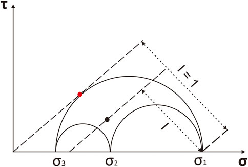
FIGURE 2. Fault instability definition [modified from Vavryčuk (2011) and Vavryčuk et al. (2013)].

Vavryčuk (2014) modified Eq. 4 so that it can be evaluated from friction coefficient (μ), shape ratio (R), and directional cosines (n). Directional cosines (n) define the fault plane inclination from the regional stress axes. The modified equation is as follows:

$I=\frac{\tau -\mu \left(\sigma -1\right)}{\mu +\sqrt{1+{\mu }^2}},(5)$

where σ and τ are

$\sigma =n_1^2+\left(1-2R\right)n_2^2-n_3^2,(6)$

$\tau =\sqrt{n_1^2+{\left(1-2R\right)}^2{n}_2^2+n_3^2-{\sigma }^2}.(7)$

Aside from μ, R, and n, a regional stress (maximum horizontal stress) orientation is also important in fault instability calculations, specifically in calculating n. The slip direction (rake) of the observed fault plane is assumed to be parallel to the maximum horizontal stress (S_H) (Kinoshita et al., 2019). The S_H orientation is incorporated in n, as shown in Eq.8 (n for strike-slip regime S_H > S_v > S_h):

$\mathbf{n}=\left(n_1,n_2,n_3\right)={\left(-\sin \delta \sin \alpha ,\cos \delta ,\sin \delta \cos \alpha \right)}^T,(8)$

where δ is the observed fault plane’s dip and α is the observed fault plane’s strike subtracted by S_H. We applied Eq. 5 in this study to analyze the instability of faults related to the Pidie Jaya earthquake.

Regional Stress Parameter

Regional stress information is needed to calculate fault instability. Thus, appropriate regional stress data should be calculated or inferred carefully. The stress inversion of focal mechanism data could be applied to obtain regional stress data, typically the orientation (Vavryčuk, 2014). In our study area (the North Sumatra Basin, see Figure 3A), it was not possible to infer the in situ stress using focal mechanism; this was mainly due to the small number of available earthquake focal mechanisms within a wide time span. Hence, in this study, we inferred the stress orientation and magnitude from existing studies.

FIGURE 3

FIGURE 3. (A) Sumatra tectonic setting (modified from Barber et al. (2005)), well field location (Mount and Suppe, 1992; Hennings et al., 2012), regional station networks (open triangle), and research area (red square). (B) GCMT events from June 1976 until the M6.5 Pidie Jaya 2016 earthquake. (C) ΔCFS resolved on Panteraja structure. Depth 20 km, μ 0.4. The transparent focal mechanisms showing the selected nodal plane, used as ΔCFS source faults.

The present-day maximum horizontal stress (S_H) orientation is generally assumed to be aligned with the plate convergence vector. For instance, Kinoshita et al. (2019) used this assumption in their study of slip tendency at the forearc area of the Nankai Zone. In Sumatra, the relative plate convergence vector defined from Global Positioning System (GPS) data is N14°E (Sieh and Natawidjaja, 2000). However, studies show that, on a local scale, Sumatra’s SH does not strictly align with N14°E. From the focal mechanism inversion, Sahara et al. (2018) found a variation of the SH orientation at −1° to 2.2°N of the GSF, i.e., N12°E ± 12°, N32°E ± 10°, and N10°E ± 10° from −1° to 2.2°N, respectively. Mount and Suppe (1992) observed an arc-normal SH orientation at the back-arc basin. They found that borehole breakouts in central and southern Sumatra oil field basins show consistent elongation of the maximum horizontal stress at N39°E ± 3.9° and N50°E ± 4.1°, respectively. Though not strictly parallel with the plate convergence vector (N14°E), Mount and Suppe (1992) suggested that strong coupling between the subducting Indo-Australian Plate and overriding Sunda Plate is the underlying force in these basins. Tingay et al. (2010) suggested the orientation in these areas is perpendicular to the adjacent subduction zone, which is slightly oriented NNE-SSW in northern Sumatra and primarily oriented NE-SW in the central to the southern part.

The Pidie Jaya earthquake occurred in the back-arc basin of the northern part of Sumatra Island. Due to lack of local SH information about this area, we inferred the S_H orientation from the nearest basin, that is, from the central Sumatra Basin, to be N39°E ± 3.9° (Mount and Suppe, 1992). In this calculation, we considered the uncertainty range (±3.9°) to cover the possibility of SH which may be less than N39°E in our study area. We inferred the stress magnitude from the in situ stress measurement in the Suban field, South Sumatra, i.e., SH 340 bar/km, Sv 240 bar/km, and Sh 180 bar/km (Hennings et al., 2012).

Parameters of Panteraja and Samalanga-Sipopok Faults

For the first objective in this study, we aim to conduct a fault instability analysis of the Pidie Jaya earthquake to locate the possible causative fault. We took two faults related to the possible causative fault into consideration: the Samalanga-Sipopok and the Panteraja Faults. The strike of the Samalanga-Sipopok Fault was approximately ∼180° (Barber et al., 2005). The strike and dip of the Panteraja Fault were inferred from Pijay-Net aftershock distribution done by Muzli et al. (2018). The uncertainty was approximated from the width of the aftershock distribution, as shown in Figure 4. We found that the strike is 43.6° ± 4.7° and the dip is 61.2° ± 1.6°. Due to the lack of knowledge about the fault dip for the Samalanga-Sipopok Fault, we calculated fault instability of all possible dips (0°–90°) for both faults.

FIGURE 4

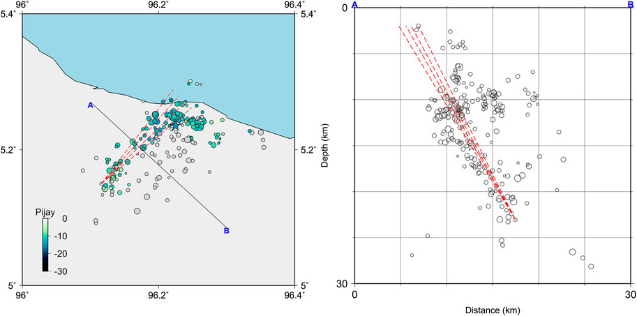
FIGURE 4. Strike and dip estimation of Panteraja Fault based on the 2016 Pidie Jaya aftershock distribution (Muzli et al., 2018). The star depicts Pidie Jaya mainshock from the Global Centroid Moment Tensor.

For the fault’s friction coefficient (µ), we estimated the maximum friction coefficient from the Mohr diagram of the stress magnitude data (SH 340 bar/km, Sv 240 bar/km, Sh 180 bar/km). We found that the failure line is tangent to this Mohr circle at µ of 0.32. Though this value might represent the principle fault's friction coefficient at the place where this data is taken, we still used it as a constraint for estimating the maximum value that we should consider in this study. In addition to the maximum friction coefficient, we also used several smaller friction coefficient values: 0.30 and 0.28.

The M6.5 Pidie Jaya Earthquake Slip Model and the Focal Mechanisms of the Aftershocks

In the second objective, we aimed to compare fault instability and ΔCFS results to the Pidie Jaya aftershocks. We calculated the fault instability of the focal mechanisms of the Pidie Jaya aftershocks. For the ΔCFS, we calculated the stress change imparted by the Pidie Jaya mainshock to the aftershock focal mechanisms. We used Coulomb3.3 software (Lin and Stein, 2004; Toda et al., 2005; Toda et al., 2011) to calculate the ΔCFS. We assessed both the nodal planes of the focal mechanism in the fault instability as well as the ΔCFS calculation. The Pidie Jaya mainshock slip model and focal mechanisms we used (Figure 5) refer to the results of Muzli et al. (2018) and Rusli (2017).

FIGURE 5

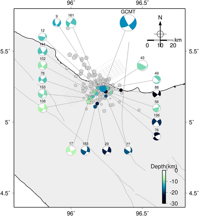
FIGURE 5. Events, focal mechanisms, and slip model grid (green and blue lines) of the 2016 Pidie Jaya aftershocks used in this study refer to the results of Supendi et al. (2017), Muzli et al. (2018), and Rusli (2017).

The focal mechanisms of the Pidie Jaya aftershocks might provide additional focal mechanism data for this area. Revisiting the possibility of inverting stress orientation from focal mechanism data, we plotted the P/T axes of the focal mechanism of the Pidie Jaya aftershocks in Figure 6, using STRESSINVERSE code (Vavryčuk, 2014). The P/T axes of the focal mechanisms could show the direction of maximum and minimum principal stress direction acting on the focal mechanism. From Figure 6, we can see that most of the aftershocks create a convergent cluster of principal stress axes; however, some points deviate, which is shown by red open circles in the lower half-circle and blue positive signs in the left half-circle. This deviation might show slight variation in the direction of local stress acting on the focal mechanisms. The azimuth of (average) maximum principal stress or sigma 1 is oriented approximately NNW, as shown by the green dot in Figure 6. The orientation of maximum principal stress could represent the SH direction. However, in this case, inverting stress orientation from aftershock data might represent the local stress orientation as the result of the mainshock stress perturbation. Thus, we did not invert the regional stress orientation from the focal mechanism of the Pidie Jaya aftershocks.

FIGURE 6

FIGURE 6. P/T axes of Pidie Jaya aftershock focal mechanisms.

Results

Sumatra Regional Stress Analysis

Vavryčuk (2011) suggests that the major earthquake could impart large stress perturbation which might rotate the orientation of the regional stress. Therefore, it is necessary to analyze the possible stress rotation in the study region. Stress rotation can be observed indirectly from ΔCFS distribution. When the earthquake's stress drop is much larger than the regional deviatoric stress, the optimum slip planes near the fault might be rotated (King et al., 1994).

For that purpose, we conducted a ΔCFS analysis of the major events preceding the Pidie Jaya earthquake. The nearest stress perturbation source in our study area comes from GSF activity in northern Sumatra. Therefore, we conducted static ΔCFS preanalysis using these events. GSF focal mechanisms data during the period of June 1976–December 2016 were compiled from the Global Centroid Moment Tensor Catalog (Figure 3B). We estimated the ΔCFS and found that ΔCFS stress change is small in the target study area (less than 1 bar), as shown in Figure 3C. Thus, the SH rotation due to GSF events is likely insignificant in our study area.

Another possible stress perturbation source arises from subduction zone activity, especially the 2004 Sumatra-Andaman M 9.2 earthquake. Hardebeck (2012) analyzed the stress rotation due to the Sumatra-Andaman earthquake in its rupture zone area, excluding inland Sumatra. Hardebeck found that the earthquake generates stress rotation in the rupture zone which rotated back after several months in the southern rupture zone area (≈2°–5°N). In addition, Rafie et al. (2019) analyzed stress rotation in inland Sumatra. The moderate rotation was found in the northern part of GSF (≈3°–6°N), yet Rafie et al. noted that this result should be cautiously interpreted because of limited available input data (earthquake data). Our study area (4.5°–5.5°N) is in the Northern Sumatra Basin and is off the GSF; therefore, the impact of the megathrust event might be even lower. Moreover, though the area might be exposed to stress rotation, there is a possibility of return rotation to occur.

Fault Instability of Panteraja and Samalanga-Sipopok Faults

We calculated the fault instability of the Panteraja and Samalanga-Sipopok Faults using approximated strikes of 43.6° and 180° for each fault. The maximum horizontal stress orientation we used is N39° ± 3.9°E and the magnitudes are SH 340 bar/km, Sv 240 bar/km, and Sh 180 bar/km. We varied the friction coefficient into three values: 0.32, 0.30, and 0.28. The results based on these input parameters are plotted in Figure 7. The right pane shows instability vs. dip values, while the left pane shows the Mohr diagram for strike and dip combinations in the right pane. Though the Samalanga-Sipopok Fault has higher instability in these figures, we could see that the Panteraja Fault also shows increasing instability values at dips of 40°–70° regardless of the friction coefficient. Optimum dip values for the Panteraja Fault to undergo a slip in this case might lie in dips of ≈40°–70°. Moreover, the Pidie Jaya aftershock distribution shows a dip of 61.2° ± 1.6°, which lies inside the optimum dip values. The higher instability values of the Samalanga-Sipopok Fault might be related to the slip of preceding events, e.g., the mb 6.1 1967.

FIGURE 7

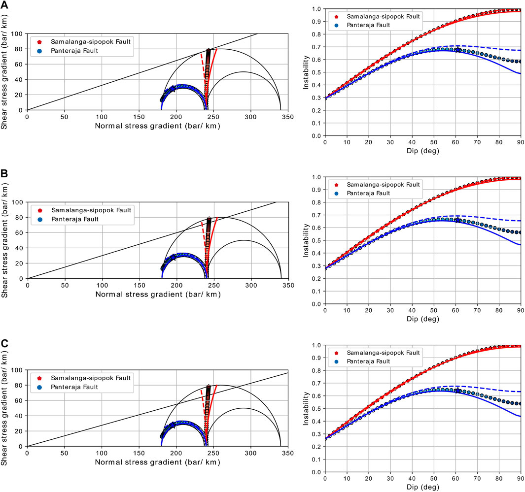
FIGURE 7. Instability results with constant strike values 43.6° for Panteraja and 180° for Samalanga-Sipopok Faults. Dip values were varied from 0° to 90°. The coefficient friction (μ) is 0.32 for (A), 0.30 for (B), and 0.28 for (C). The right pane is instability vs. dip values and the left pane is the Mohr diagram. Regional maximum horizontal stress orientation is N39° ± 3.9°E; N35.1°E for the dashed line, and N42.9°E for the solid line, but N39°E for the pentagon and circle line. Star shows Panteraja Fault with strike 43.6° and dip 61.2°.

Instability, as shown in Figure 7, is plotted with varying friction coefficients but constant SH values. Hence, the Mohr circle is intersected at two points with the failure line. In real conditions, the Mohr circle will decrease and become tangent only to the failure line at one point. Therefore, we again calculated the instability of the Panteraja Fault with a smaller SH magnitude, utilizing Eq. 9:

$\sin \psi = \frac{\left(1/2\right)\left(\text{SH}-\text{Sh}\right)}{\left(1/2\right)\left(\text{SH}+\text{Sh}\right)},(9)$

where ѱ is the arcus tangent of the friction coefficient, which we varied into 0.32, 0.30, and 0.28. We found that decreases in SH magnitude will cause a slight increase in the peak of instability curve of the Panteraja Fault, as shown in Figure 8.

FIGURE 8

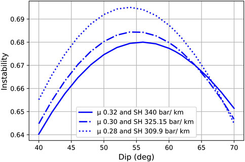
FIGURE 8. Instability of Panteraja Fault at dips of 40°–70°, using different friction coefficients and SH magnitudes. The Sv, Sh magnitudes, SH orientation, and strike of Panteraja Fault are kept constant: Sv 240 bar/km, Sh 180 bar/km, N39°E, and 43.6°, respectively. The stress magnitudes refer to Hennings et al. (2012), while the stress orientation refers to Mount and Suppe (1992).

Fault Instability and ΔCFS in M6.5 Pidie Jaya Aftershocks

Fault instability was calculated on both nodal planes of the Pidie Jaya aftershocks in Figure 5. We grouped the nodal planes into NE-SW and NW-SE based on their strike orientation. Using the nodal plane parameter, we calculated instability for each event and plotted these in the Mohr diagram in Figure 9A. The majority of the aftershocks have higher instability for NE-SW nodal planes, except for events 9 and 12 (Figure 9B)). In the Mohr diagram, these NE-SW nodal planes are clustered mostly near the left inner circle where the mainshock would be, as seen in Figure 7. We also calculated ΔCFS as imparted by the mainshock to the NE-SW and NW-SE aftershock nodal planes. Most of the aftershocks experienced stress change in the range of ±1 bar. We plotted the ΔCFS results in Figure 9C. The friction coefficient used to generate results in Figure 9 is 0.32. We only used µ 0.32, because we found that smaller friction coefficients (0.30 and 0.28) in this case did not flip the result. The list of nodal planes and the results are in Supplementary Table S1.

FIGURE 9

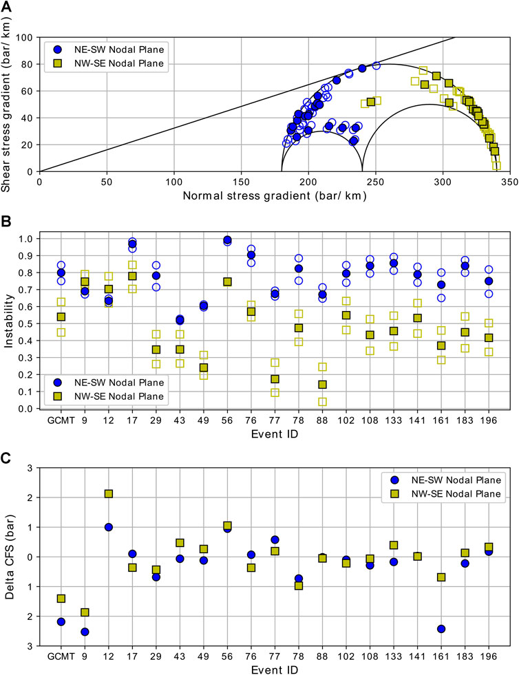
FIGURE 9. Instability of NE-SW and NW-SE aftershock focal mechanism nodal planes plotted in Mohr diagram (A) and in a graph of instability vs. event number (B). The ΔCFS of 2016 Pidie Jaya mainshock resolved in the NE-SW and NW-SE aftershock focal mechanism nodal planes (C). The open blue circle and yellow square in (A) and (B) are instability values calculated using SH N35.1°E and N42.9°E. The others are calculated using SH N39°E.

Discussion

The seismic history of the northern Sumatra region was analyzed by Hurukawa et al. (2014), who gathered and relocated historical earthquake data along the Sumatran Fault up to 2012. In the northern part of Sumatra, events from 1935 to 2012 were detected in the Hurukawa Catalog. The 1967 mb 6.1 earthquake occurred near the 2016 Pidie Jaya earthquake. The 1967 earthquake moved closer to the Samalanga-Sipopok Fault after relocation. We suggest the 1967 event to be related to Samalanga-Sipopok Fault activity. Other than the 1967 event, there is no historical M ≥ 6.0 earthquake recorded by the catalog around the Samalanga-Sipopok or Panteraja Faults (Supplementary Figure S1).

Based on GPS observations, the northern part of GSF has slip rates ranging between 16 and 20 mm/year (Ito et al., 2012). By using these slip rates as estimated slip rates for the Samalanga-Sipopok and Panteraja Faults, we were able to estimate the accumulated slip on these faults. The mb 6.1 1967 was the oldest event near the Samalanga-Sipopok Fault, as recorded in the Hurukawa Catalog. Thus, the accumulated slip of the Samalanga-Sipopok Fault from 1967 up to 2016 is approximately 0.78–0.98 m. Regarding the Panteraja Fault, there is no historically large event (M ≥ 6.0) in northern Sumatra recorded in the years spanning 1935–2012. Roughly estimated, the approximated accumulated slip of the Panteraja Fault since 1935–2016 is 1.30–1.62 m. It is worth noting that, given the limited seismic catalog we have for northern Sumatra, 1.30–1.62 m is the possible lower limit of slip accumulation in the Panteraja Fault. Nonetheless, from these calculations, we could see that Panteraja Fault has a larger accumulated slip than Samalanga-Sipopok Fault; hence, it is building up more stress than the Samalanga-Sipopok Fault, making it more susceptible for an earthquake occurrence.

A fault with a higher instability value is more susceptible to undergo slip. From Figure 7, we see that the Samalanga-Sipopok Fault has higher instability values than the Panteraja Fault. However, the Panteraja Fault has a unique fault instability feature. The instability curve peaked at a dip range between 40° and 70°, reaching the maximum values. This dip range might be revealing the most optimum dip for the Panteraja Fault to have an earthquake; the reactivated structure for the Pidie Jaya 2016 earthquake has a dip value of 61.2° ± 1.6°, which coincides with the optimum dip range. Based on the seismic history and the fault instability analysis, we suggest that Panteraja was the causative fault plane of the 2016 Pidie Jaya earthquake.

In attempting to resolve the ΔCFS on the aftershock focal mechanism nodal planes, one should infer the fault plane carefully because if one nodal plane has a positive stress change, the other may have a negative stress change (Toda et al., 2011). Thus, Toda et al. (2011) suggest that the fault plane should be inferred, based on independent information such as seismic alignment. While for fault instability calculation, local redistribution of Coulomb stress might activate a cluster of events with slightly low instability values, as suggested by Vavryčuk et al. (2013) in their study using swarm events. Indeed, analysis of the Pidie Jaya aftershock fault instability and ΔCFS comparison should be carried out cautiously. Therefore, we used the aftershock alignments to further confirm the results.

Recalling the instability result in Figure 9B, most of the NE-SW nodal planes have higher instability, except for events 9 and 12 which have slightly smaller instability at the NE-SW orientation. Then, we tried to plot the aftershocks focal mechanisms with the NE-SW nodal planes highlighted, in Figure 10. We also colored the focal mechanisms in this figure based on the ΔCFS result for the NE-SW nodal plane. Particularly for events 9 and 12, we plotted the NW-SE nodal plane and their ΔCFS results. Faults with higher instability are interpreted as faults which are more susceptible to failure. In the case of the Pidie Jaya aftershock focal mechanisms, we suggest that they failed in the NE-SW nodal plane. This is because the main fault of the mainshock ruptured in the NE-SW direction, as shown by the sharp alignment of local events and GPS observation. Gunawan et al. (2020) found that, by using the NE-SW fault plane orientation that extends to the offshore as the mainshock, the synthetic and observed displacement in nearby GPS stations fits very well. However, for events 9 and 12, the failure plane might be flipped to NW-SE. The first week aftershocks recorded by the BMKG regional network show sparse NW-SE event orientation. Approximately 78.4% of these regional aftershocks are concentrated in depths of 0 –15 km. Events 9 and 12 are located at the northern tip of the local aftershocks; they have shallow depths and occurred eight days after the mainshock. We suggest that there may have been a possible conjugate failure at a shallow depth in the NW-SE direction (aside from the NE-SW main fault failure), in which events 9 and 12 might have failed. This might confirm the identified cracks which are once thought to be associated with the possible NW-SE mainshock fault plane (right-lateral faulting) (National Center for Earthquake Studies of Indonesia (PUSGEN), 2017) but later suspected as the secondary effect of the NE-SW mainshock fault plane (Gunawan et al., 2020).

FIGURE 10

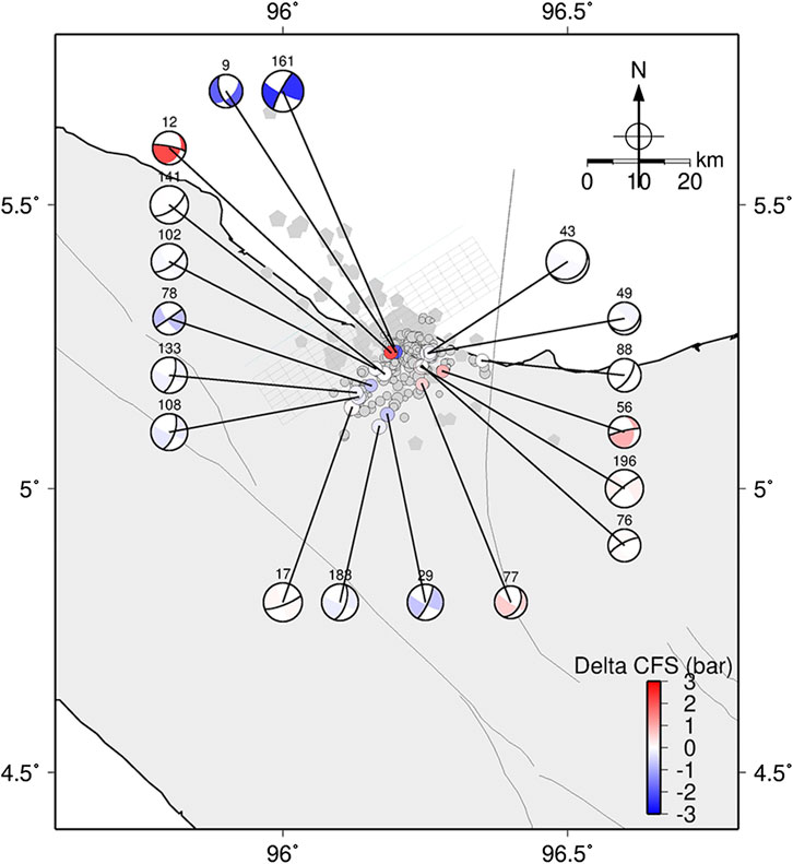
FIGURE 10. Map view of the ΔCFS of 2016 Pidie Jaya main shock resolved in the NE-SW aftershock focal mechanism nodal planes; except for events 9 and 12. The focal mechanisms are colored, based on the ΔCFS value. Bold nodal lines are the chosen nodal planes. Numbers above the focal mechanisms show the event number.

The ΔCFS and fault instability comparison for each aftershock (marked as aftershock event numbers) is plotted in Figure 11. From the comparison, we found that fault instability and ΔCFS do not have similar trends. However, the comparison showed that some of the events with negative ΔCFS have high instability values (above 0.7). This might give insight regarding the occurrence of events in the negative ΔCFS. The Coulomb stress is not sufficient to trigger other events in the negative ΔCFS area, yet some events occurred there, as can be seen in Figure 10. These events might exist as they are optimally oriented beforehand, which is shown from their high instability value.

FIGURE 11

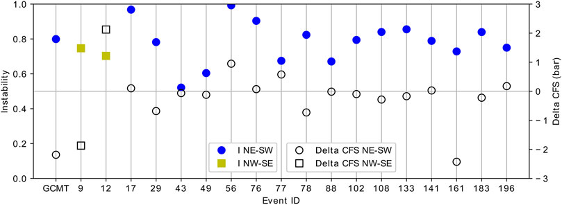
FIGURE 11. Comparison of instability and ΔCFS of Pidie Jaya aftershocks nodal planes. All events, except events 9 and 12, are plotted using their NE-SW instability and ΔCFS results. Both instability and ΔCFS calculation used a friction coefficient of 0.32.

Conclusion

We have conducted a fault instability analysis of the Pidie Jaya earthquake and described its relation to ΔCFS distribution. By using the fault instability method for the Pidie Jaya causative fault analysis, we concluded that neither the fault responsible for the 1967 mb 6.1 event nor the Samalanga-Sipopok Fault is the causative fault; however, we strengthened the Panteraja Fault as the causative fault, due to its dip which coincides with the optimum dip range.

Aftershock events located in the stress shadows were found to have a quite high fault instability, which indicates that these are the reactivation of critically stressed fractures (Figure 11). Therefore, we showed that fault instability of the preexisting fractures plays a role in inhibiting or promoting the occurrence of aftershock events.

The GSF is a well-documented active Fault in Sumatra. Besides the GSF, northern Sumatra is also exposed to off-GSF faults, i.e., the Panteraja, Samalanga-Sipopok, and Lhoksemauwe Faults (Barber et al., 2005). Several historical earthquakes, as well as recent earthquakes, were located around these faults, indicating that these off-GSF faults are also active. Moreover, our fault instability calculation has shown that the off-GSF (Panteraja and Samalanga-Sipopok) faults are unstable in the Sumatra regional stress setting. This is shown by the high instability value, thereby making it more susceptible for slip movement, stress build-up, and finally fault failure (earthquakes), which could occur in its return period (Hardebeck and Okada, 2018).

Data Availability Statement

The datasets generated for this study are available on request to the corresponding author.

Author Contributions

DK and DS contributed to modeling, result analysis, and manuscript writing. MM contributed to data preparation. SW, AN, MM, II, NP, and ZZ reviewed the manuscript. All authors have read and approved the final manuscript.

Funding

The authors would like to thank the Institut Teknologi Bandung (ITB) for supporting this research through “Program Riset Unggulan ITB 2019” managed by the Research Center for Disaster Mitigation (PPMB), ITB.

Conflict of Interest

The authors declare that the research was conducted in the absence of any commercial or financial relationships that could be construed as a potential conflict of interest.

Acknowledgments

We used Generic Mapping Tools (Wessel and Smith, 1998) to produce most of the figures. In addition, several figures were produced using Matplotlib (Hunter, 2007). This work was partially funded by the Ministry of Research, Technology, and Minister of Education of Indonesia under WCU 2020 Program managed by ITB awarded to S. Widiyantoro. We thank YZ, VV and FB as the reviewer and BT as the editor who gave constructive suggestions and advices.

Supplementary Material

The Supplementary Material for this article can be found online at: https://www.frontiersin.org/articles/10.3389/feart.2020.559434/full#supplementary-material.

References

Barber, A. J., Crow, M. J., and Milsom, J. (2005). Sumatra: geology, resources and tectonic evolution. Geological Magazine. 143 (6), 933. doi:10.1017/s0016756806212974

CrossRef Full Text | Google Scholar

Cameron, N. R., Bennett, J. D., Bridge, D. M., Clarke, M. G. C., Djunuddin, A., Ghazali, S. A., et al. (1983). The Geology of the Takengon Quadrangle (0520), Sumatra. Scale 1: 250 000. Geological Research and Development Centre, Bandung, 284.

CrossRef Full Text | Google Scholar

Djatmiko, H. T. (2016). Gempabumi kuat M=6.5 guncang Pidie Jaya, provinsi Aceh dipicu akibat aktivitas sesar aktif. (in Indonesian). https://www.bmkg.go.id/press-release/?p=gempabumi-kuat-m6-5-guncang-pidie-jaya-provinsi-aceh-dipicu-akibat-aktivitas-sesar-aktif&tag=press-release&lang=ID. (last accessed December 27, 2019).

CrossRef Full Text | Google Scholar

Genrich, J., Bock, Y., Mccaffrey, R., Prawirodirdjo, L., Stevens, C., Puntodewo, S., et al. (2000). Distribution of slip at the northern Sumatran Fault System. J. Geophys. Res.: Solid Earth. 105 (B12), 28327–28341. doi:10.1029/2000JB900158

CrossRef Full Text | Google Scholar

Gunawan, E., Nishimura, T., Susilo, S., Widiyantoro, S., Puspito, N. T., Sahara, D. P., et al. (2020). Fault source investigation of the 6 December 2016 Mw 6.5 Pidie Jaya, Indonesia, earthquake based on GPS and its implications of the geological survey result. J. Appl. Geodes. 14 (4), 405–412. doi:10.1515/jag-2020-0027

CrossRef Full Text | Google Scholar

Hardebeck, J. L. (2012). Coseismic and post-seismic stress rotations due to great subduction zone earthquakes. Geophys. Res. Lett. 39, L21313. doi:10.1029/2012GL053438

CrossRef Full Text | Google Scholar

Hardebeck, J. L., and Okada, T. (2018). Temporal stress changes caused by earthquakes: a review. J. Geophys. Res.: Solid Earth. 123, 1350–1365. doi:10.1002/2017jb014617

CrossRef Full Text | Google Scholar

Harris, R. A. (2000). Earthquake stress triggers, stress shadows, and seismic hazard. Curr. Sci. 79 (9), 1215–1225.

CrossRef Full Text | Google Scholar

Hennings, P., Allwardt, P., Paul, P., Zahm, C., Reid, R., Alley, H., et al. (2012). Relationship between fractures, fault zones, stress, and reservoir productivity in the Suban gas field, Sumatra, Indonesia. AAPG Bulletin. 96 (4), 753–772. doi:10.1306/08161109084

CrossRef Full Text | Google Scholar

Hunter, J. D. (2007). Matplotlib: a 2D graphics environment. Comput. Sci. Eng. 9, 90–95. doi:10.1109/mcse.2007.55

CrossRef Full Text | Google Scholar

Hurukawa, N., Wulandari, B. R., and Kasahara, M. (2014). Earthquake history of the Sumatran fault, Indonesia, since 1892, derived from relocation of large earthquakes. Bull. Seismol. Soc. Am. 104, 1750–1762. doi:10.1785/0120130201

CrossRef Full Text | Google Scholar

Ito, T., Gunawan, E., Kimata, F., Tabei, T., Simons, M., Meilano, I., et al. (2012). Isolating along-strike variations in the depth extent of shallow creep and fault locking on the northern Great Sumatran Fault. J. Geophys. Res. 117, B06409. doi:10.1029/2011JB008940

CrossRef Full Text | Google Scholar

Keats, W., Cameron, N. R., Djunuddin, A., Ghazali, S.A., Harahap, H., Kartawa, W., et al. (1981). The Geology of the Lhokseumawe Quadrangle, Sumatra. Geological Research and Development Centre, Bandung. [Explanatory note, 13 pp., and geological map, quadrangle 0521, 0621.

CrossRef Full Text | Google Scholar

King, G. C. P., Stein, R. S., and Lin, J. (1994). Static stress changes and the triggering of earthquakes. Bull. Seismol. Soc. Am. 84, 935–953.

CrossRef Full Text | Google Scholar

Kinoshita, M., Shiraishi, K., Demetriou, E., Hashimoto, Y., and Lin, W. (2019). Geometrical dependence on the stress and slip tendency acting on the subduction megathrust of the Nankai seismogenic zone off Kumano. Progress in Earth and Planetary Science. 6, 7. doi:10.1186/s40645-018-0253-y

CrossRef Full Text | Google Scholar

Kusumawati, D., Sahara, D., Nugraha, A., and Puspito, N. (2019a). “Stress drop, earthquake aftershocks and regional stress relation based on synthetic static Coulomb failure stress model,” J. Phys. in Conference Series. 1204, 012092. (Bristol, United Kingdom: IOP Publishing). doi:10.1088/1742-6596/1204/1/012092

CrossRef Full Text | Google Scholar

Kusumawati, D., Sahara, D. P., Nugraha, A. D., and Puspito, N. T. (2019b). Sensitivity of static Coulomb stress change in relation to source fault geometry and regional stress magnitude: case study of the 2016 Pidie Jaya, Aceh earthquake (Mw= 6.5), Indonesia. J. Seismol. 23 (6), 1391–1403. doi:10.1007/s10950-019-09878-3

CrossRef Full Text | Google Scholar

Leclère, H., and Fabbri, O. (2013). A new three-dimensional method of fault reactivation analysis. J. Struct. Geol. 48, 153–161. doi:10.1016/j.jsg.2012.11.004

CrossRef Full Text | Google Scholar

Lin, J., and Stein, R. S. (2004). Stress triggering in thrust and subduction earthquakes, and stress interaction between the southern San Andreas and nearby thrust and strike-slip faults. J. Geophys. Res. 109, B02303. doi:10.1029/2003JB002607

CrossRef Full Text | Google Scholar

Morris, A., Ferrill, D. A., and Henderson, D. B. (1996). Slip-tendency analysis and fault reactivation. Geology. 24, 275–278.

CrossRef Full Text | Google Scholar

Mount, V. S., and Suppe, J. (1992). Present-day stress orientations adjacent to active strike-slip faults: California and Sumatra. J. Geophys. Res.: Solid Earth. 97, 11995–12013.

CrossRef Full Text | Google Scholar

Muzli, M., Umar, M., Nugraha, A. D., Bradley, K. E., Widiyantoro, S., Erbas, K., et al. (2018). The 2016 M w 6.5 Pidie Jaya, Aceh, North Sumatra, earthquake: reactivation of an unidentified sinistral fault in a region of distributed deformation. Seismol Res. Lett. 89, 1761–1772. doi:10.1785/0220180068

CrossRef Full Text | Google Scholar

National Center for Earthquake Studies of Indonesia (PUSGEN) (2017). Investigation on the Pidie Jaya earthquake in Aceh province (in Bahasa Indonesia). Indonesia: Research and Development Agency of Ministry of Public Work and Housing.

CrossRef Full Text | Google Scholar

Oppenheimer, D. H., Reasenberg, P. A., and Simpson, R. W. (1988). fault plane solutions for the 1984 morgan hill, California, earthquake sequence: evidence for the state of stress on the calaveras fault. J. Geophys. Res.: Solid Earth. 93, 9007–9026. doi:10.1029/JB093iB08p09007

CrossRef Full Text | Google Scholar

Rafie, M. T., Sahara, D. P., Widiyantoro, S., and Nugraha, A. D. (2019). “Impact of the 2004 sumatra-andaman earthquake to the stress heterogeneity and seismicity pattern in Nothern Sumatra, Indonesia,”in IOP conference series: earth and environmental science. 318 (1), 012010 (Bristol, United Kingdom: IOP Publishing).

CrossRef Full Text | Google Scholar

Rusli, K. A. (2017). Aftershock mechanism analysis of an earthquake in Pidie Jaya Aceh december 7th, 2016. Bachelor’s thesis. (Jawa Barat, Indonesia: Institut Teknologi Bandung).

CrossRef Full Text | Google Scholar

Sahara, D. P., Kusumawati, D., Widiyantoro, S., Nugraha, A. D., Zulfakriza, , and Puspito, N. T. (2019). “Preliminary Fault instability analysis of M6.5 Pidie Jaya, Aceh 2016 earthquake,” in Advances in science, technology and innovation. (Berlin, Germany: SpringerLink) [accepted].

CrossRef Full Text | Google Scholar

Sahara, D. P., Widiyantoro, S., and Irsyam, M. (2018). Stress heterogeneity and its impact on seismicity pattern along the equatorial bifurcation zone of the Great Sumatran Fault, Indonesia. J. Asian Earth Sci. 164, 1–8. doi:10.1016/j.jseaes.2018.06.002

CrossRef Full Text | Google Scholar

Sibson, R. H. (1985). A note on fault reactivation. J. Struct. Geol. 7, 751–754. doi:10.1016/0191-8141(85)90150-6

CrossRef Full Text | Google Scholar

Sibson, R. H. (1990). Rupture nucleation on unfavorably oriented faults. Bull. Seismol. Soc. Am. 80, 1580–1604.

CrossRef Full Text | Google Scholar

Sieh, K., and Natawidjaja, D. (2000). Neotectonics of the Sumatran Fault, Indonesia. J. Geophys. Res. 105, 28295–28326.

CrossRef Full Text | Google Scholar

Supendi, P., Nugraha, A. D., and Wijaya, T. A. (2017). Relocation and focal mechanism of aftershocks Pidie Jaya earthquake (Mw6. 5) dec 7th, 2016 using BMKG network. Jurnal Geofisika. 15, 17–20. doi:10.36435/jgf.v15i1.19

CrossRef Full Text | Google Scholar

Tingay, M., Morley, C., King, R., Hillis, R., Coblentz, D., and Hall, R. (2010). Present-day stress field of southeast asia. Tectonophysics. 482, 92–104. doi:10.1016/j.tecto.2009.06.019

CrossRef Full Text | Google Scholar

Toda, S., Stein, R. S., Richards-Dinger, K., and Bozkurt, S. (2005). Forecasting the evolution of seismicity in southern California: animations built on earthquake stress transfer. J. Geophys. Res. 110, B05S16. doi:10.1029/2004JB003415

CrossRef Full Text | Google Scholar

Toda, S., Stein, R. S., Sevilgen, V., and Lin, J. (2011). Report 2011-1060. Coulomb 3.3 Graphic-rich deformation and stress-change software for earthquake, tectonic, and volcano research and teaching—user guide (U.S. Geological Survey Open-File), 63. Available at http://pubs.usgs.gov/of/2011/1060/

CrossRef Full Text | Google Scholar

Tong, H., and Yin, A. (2011). Reactivation tendency analysis: a theory for predicting the temporal evolution of preexisting weakness under uniform stress state. Tectonophysics. 503, 195–200. doi:10.1016/j.tecto.2011.02.012

CrossRef Full Text | Google Scholar

Vavryčuk, V., Bouchaala, F., and Fischer, T. (2013). High-resolution fault image from accurate locations and focal mechanisms of the 2008 swarm earthquakes in West Bohemia, Czech Republic. Tectonophysics. 590, 189–195. doi:10.1016/j.tecto.2013.01.025

CrossRef Full Text | Google Scholar

Vavryčuk, V. (2011). Principal earthquakes: theory and observations from the 2008 west bohemia swarm. Earth Planet Sci. Lett. 305, 290–296. doi:10.1016/j.epsl.2011.03.002

CrossRef Full Text | Google Scholar

Vavryčuk, V. (2014). Iterative joint inversion for stress and fault orientations from focal mechanisms. Geophys. J. Int. 199 (1), 69–77. doi:10.1093/gji/ggu224

CrossRef Full Text | Google Scholar

Wessel, P., and Smith, W. H. F. (1998). New, improved version of generic mapping tools released. Eos, Transactions American Geophysical Union. 79, 579. doi:10.1029/98EO00426

CrossRef Full Text | Google Scholar

Zoback, M. D. (2007). Reservoir geomechanics. Cambridge, United Kingdom: Cambridge University Press. doi:10.1017/CBO9780511586477

CrossRef Full Text | Google Scholar