Soil Solution Analysis With Untargeted GC–MS—A Case Study With Different Lysimeter Types

Introduction

Mobile organic compounds in surface and subsurface compartments, also called dissolved organic matter (DOM), are valuable markers for the monitoring of water fluxes, water quality, and pollution (Bianchi and Canuel, 2011). These surface signals can be altered or transformed but hardly traced within the Critical Zone (Küsel et al., 2016). The main groundwater recharge mechanism is the infiltration of precipitation and percolation of the seepage solution through soils (Freeze, 1969). Previous studies on DOM focused mainly on deposition, contamination, migration, and transformation of pollutants, such as polycyclic aromatic hydrocarbons, dioxins or insecticides (Frimmel et al., 2002; Haarstad et al., 2012). In contrast, natural organic signatures in uncontaminated environments are rather poorly understood, though there is a huge interest in quantifying such carbon compounds in soil solution, particularly to elucidate the formation and breakdown of organic matter in groundwater. Due to low concentrations and high chemical diversity of such compounds, untargeted sampling and analysis is highly challenging. Consequently, most existing methods focus on the targeted quantification of specific compounds with elaborate compound specific extraction steps (Fenoll et al., 2011). Untargeted approaches are a growing field for DOM analysis. The majority of these methods focus on compound classes (Brock et al., 2020; Ye et al., 2020) or they calculate sum formulas for more precise data annotation (Thieme et al., 2019). Still underrepresented are publications covering compound identification despite the fact that they have the potential to give novel insights into complex environmental processes including microbial and abiotic transformations (Bundy et al., 2009; Leyva et al., 2020; Withers et al., 2020). Metabolomics techniques have now matured sufficiently to serve as a tool for monitoring environmental samples (Garcia-Sevillano et al., 2015). Progress has been made in the high-resolution Fourier-transform mass spectrometry-based characterization of metabolic patterns in groundwater (Brown et al., 2005; Tautenhahn et al., 2012; Roth et al., 2015). These studies provide information on the elemental composition of analytes and allow correlation of observed patterns to the prevalence of substance classes. Another powerful approach is the use of hyphenated techniques where chromatographic methods are coupled to mass spectrometry (MS) allowing the sensitive detection and quantification of a broad range of metabolites. In both approaches it is however a challenge to spot relevant peaks from environmental samples in the presence of dominant contaminants. The availability of elaborate algorithms to filter out signals of contaminants allows tracing of biotic and abiotic signatures in even dilute matrices. Such background corrected data-sets can be the basis for comparative metabolomics as a tool to spot relevant differences in sample groups (Kuhlisch and Pohnert, 2015). Using computer-assisted statistical evaluation of datasets as well as data bases and analyzes of fragmentation patterns, relevant regulated compounds can be identified (Alonso et al., 2015). Such untargeted approaches require a rather unselective but reproducible and contamination-poor sampling that has which is problematic in the case of soil solution.

In soil sciences, percolate collecting devices are powerful tools to collect and to quantify the passing water in the soil (Robertson et al., 1999; Weihermüller et al., 2007; Singh et al., 2018). Several studies have employed devices for water extraction from soil in general (Siemens and Kaupenjohann, 2004) or for the analysis of sum parameters, such as dissolved organic matter or for the targeted analysis of specific compounds (Winton and Weber, 1996; Fischer et al., 2003; Lloyd et al., 2012; Olofsson et al., 2014). Even the term lysimeters seems to be not clearly defined; such devices have also been used to quantify the export of suspended particulates, DOM, and hydrophobic organic compounds (Totsche et al., 2007; Dibbern et al., 2014) or to trace the carbon flow in the below-ground food web (Kramer et al., 2012; Malá et al., 2013). Challenging is the aspect that usually water collecting devices are constructed to cover (hydro) geological aspects rather than the needs of highly sensitive chemical analysis (Siemens and Kaupenjohann, 2003). Such devices are often resulting substantial background signals if samples are utilized for metabolomics analyzes. Here we present the development and evaluation of different lysimeters for water collection and subsequent sample preparation with the aim to establish a robust sampling method to enable comparative investigations of organic signatures using powerful algorithms developed for metabolomics. We use a GC-MS based approach for separation and detection that focuses on comparably small and mobile compounds, however, the workflow can easily be adapted to liquid chromatography/mass spectrometry (LC-MS) as well. Particular strengths of GC-MS are 1) high chromatographic separation performance, thus low competitive effects such as ion suppression, and more facile association of signals in comparative metabolomics compared to LC-MS; 2) EI-ionisation as employed by us is a more universal ionization technique compared to ESI which relies on protonation or deprotonation sites. Intrinsic fragmentation allows the use of common databases such as NIST and fragmentation theory also supports the assignment of unknown compounds. With seepage water, where many compounds do not match to database entries, we therefore consider the GC-MS approach strong to deal with unknown metabolites and enabling follow-up identification studies.

The introduced workflow permits the identification of marker molecules characteristic for land use that can be traced below ground. It thereby opens possibilities to monitor fluxes as well as (microbial) transformation. We introduce a lysimeter that reduces background signals of contaminants to a minimum thereby facilitating easy and reliable analysis of analytical data sets. Another focus of this study is the chemoinformatic elimination of background signals, caused by plasticizers or other contaminants introduced during sampling and workup. The optimized workflow is applied for monitoring of differences in organic signatures of water samples, collected at the topsoil-subsoil boundary at three different land-use sites.

Materials and Methods

Sampling Sites

For method development, soil solution was collected at closely neighboring locations at long-term monitoring sites of the Hainich Critical Zone Exploratory (CZE) Thuringia, central Germany (Figure 1) (Küsel et al., 2016). The bedrock at the eastern hillslope of the Hainich low-mountain range is composed of alternating sequences of limestones and mudstones of Upper Muschelkalk (subgroup of Germanic Triassic) formations (Lehmann et al., 2020). Major soil types are cambisols, luvisols, and chromic cambisols that formed from the limestone-mudstone alternations and loess derivates as parent materials (Kohlhepp et al., 2017). Sampling took place at the monitoring plot transect, along the northern border of the Hainich National Park [51.105,508 N, 10.407,190 E, 440 m above sea level]. The different sites used in this study comprise the land uses: 1) managed forest of mainly European beech (Fagus sylvatica L.) with dominant cambisol soil type, 2) agricultural site with cropland used for wheat, corn, canola also dominated by a cambisol soil type, and 3) pasture site which is characterized by luvisols and chromic cambisols (Kohlhepp et al., 2017).

FIGURE 1

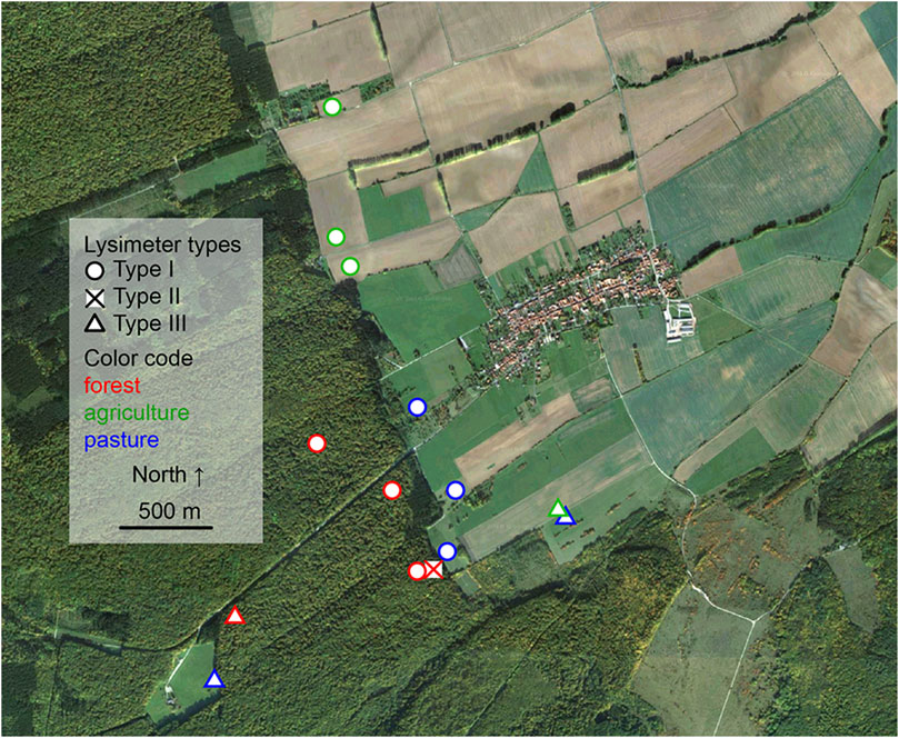
FIGURE 1. Satellite image of the sampling transects including highlighted sampling spots. “Map data: Google, DigitalGlobe 2016”.

Lysimeter Set-Up

Three different lysimeters were evaluated for the collection of soil solution exiting the topsoil horizon (Ah). The lysimeters were installed in October 2014 up to May 2015 and regular sampling (every fortnight) as well as event-based sampling, following events like thunderstorms, has been performed for this analysis from October 2015 to January 2016. Table 1 lists the specifics of the respective instruments which are shown in Figure 2. Supplementary Table S1 lists the replicates utilized within this study as well as the sampling places and times.

TABLE 1

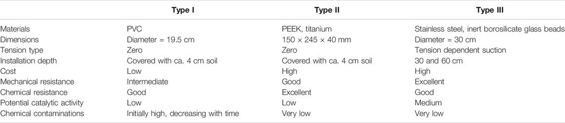
TABLE 1. Relevant features of the employed lysimeters.

FIGURE 2

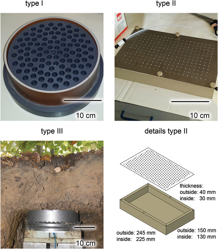
FIGURE 2. Images and technical drawing of lysimeters used in this study. Type I is made of poly vinyl chloride (PVC), type II of poly ether ether ketone (PEEK) and titanium, type III is made of stainless steel and glass.

Type I Lysimeter

This lysimeter consists of a polyvinylchloride (PVC) cylinder (diameter = 19.5 cm) and a concave bottom plate (Figure 2). The cylinder is separated by a punch plate into a bottom part, where the solution is collected gravimetrically and stored, and a top part with the forest floor/Ah soil monolith. The punch plate is perforated by 97 holes (each 10 mm in diameter) and covered by two polyethylene (PE) nets (mesh size = 0.5 mm) that prevent soil material from dropping into the collected water but allow the passage of free-draining soil solution. The solution was sampled biweekly from the bottom part by a pump via a polyethylene (PE) outlet-tube using reduced pressure and a Woulfe bottle for sample collection.

The samples for the blank signal were acquired after assembly of the lysimeter in the laboratory. First, this set-up was carefully rinsed with bidistilled water and then bidistilled water was introduced and left for one week at 20°C before sampling.

Installation

The zero-tension lysimeters were installed in July 2014 underneath the topsoil horizon so that the punch-plate of the lysimeter was covered with ca. 4 cm soil. Care was taken that the soil and the overlaying forest floor were not substantially disturbed. For lysimeter installation, a soil monolith containing the Ah soil material and the overlying forest floor layer was cut out undisturbed using a steel cylinder (diameter = 19.5 cm). Then, the soil column was carefully transferred from the steel cylinder onto the top of the net-covered punch plate of the lysimeter. The resulting soil pit was slightly enlarged and the lysimeter together with the soil monolith was installed and adjusted to the surrounding surface level. The open space between the lysimeter and the soil wall was refilled with soil material.

Type II Lysimeter

This lysimeter was prepared from a commercially available polyether ether ketone (PEEK) block with the dimensions of 150 × 245 × 40 mm. A cavity of 130 × 225 × 30 mm is milled into this block (Figure 2). The set-up is covered by a 0.6 mm thick titanium grade 1 (material number 3.7025) plate perforated with 252 holes, each with a diameter of 2 mm. These materials were selected for a minimum of potential biological activity on surface to minimize further sample modification (Zhang et al., 2014). To collect the water a 3/8–28 thread adapter for standard 1/8 inch HPLC-PTFE tubing is attached. The whole apparatus was first rinsed in the laboratory three times with bidistilled water, before being installed. Soil solution was sampled from the lysimeter by suction of the collected water using a syringe. One replicate at the time was collected and extracts were measured in triplicate with GC/MS.

Installation

The lysimeter was installed in March 2014. As described for the Type I device the installation was done by cutting and lifting the soil carefully using a sharp spade removing additional soil under the lysimeter and placing the lysimeter in parallel to the surface. Water and control sampling followed the protocol described for lysimeter type I.

Type III Lysimeter

The tension-supported Type III lysimeter was specifically constructed to representatively and quantitatively sample the seepage with dissolved, colloidal and particulate mobile components in undisturbed soils (similar Set-up: (Zhang et al., 2018). We used commercially available lysimeters that were filled with glass beads (all from UMS GmbH, München, Germany), circular in geometry and made of stainless steel (d = 0.3 m; h = 0.14 m). Hydraulic contact of the lysimeter to the soil was mediated by a porous bed made of silica beads (∼2 mm diameter, Sigmund Lindner GmbH, Warmensteinach, Germany) and supported by a 1 cm thick silicon carbide porous plate (pore size: 10 µm) at lysimeter bottom. Prior installation the system was rinsed with bidistilled water. A controlled suction is applied to the lysimeter porous plate, regulated according to the actual matric-potential measured via tensiometer (T8, UMS) in the depth of lysimeter installation (30 cm). The suction is applied with a battery powered vacuum pump, connected to a suction control unit. This unit is connected to the lysimeter via a Woulfe-bottle that collects the soil solution from the overburden undisturbed soil while at the same time applying the suction to the lysimeter.

Installation

Type III lysimeters were installed in duplicates in a depth of 30 cm (boundary topsoil-subsoil) below surface at all three land use sites. In addition, a set of duplicates in a depth of 60 cm (subsoil) was installed at the same sites. In the forest the lysimeters were installed in October 2014, in the cropland and in the pasture site in May 2015. To install a type III lysimeter a soil pit (L × W × H: 2 × 1 ×1 m) was trenched and faced. From this pit, a vertical tray (L × W × H: 0.4 × 0.4 × 0.3 m) was excavated with its top ceiling located in the desired depth for seepage water collection. In this way, the overburden soil remained undisturbed. Prior installation of the lysimeter, the tray bottom and top were carefully leveled. The lysimeter was then placed in the tray and pressed to the ceiling with the load compensation unit (Lehmann et al., 2020).

Sample Preparation

Lysimeter samples were kept at 0–5°C for transport and handled immediately in the lab. Hydrophilic-lipophilic balanced solid phase extraction (SPE) was carried out using Strata X 500 mg, 6 ml amide modified polystyrene resin cartridges (Phenomenex, Aschaffenburg, Germany) that were conditioned by passing 5 ml methanol followed by 5 ml water. For extraction, a 50 ml syringe without plunger was attached to the Luer cone of a Swinnex filter holder (Ø 47 mm, Roth, Germany) equipped with a GF/C filter (VWR, Germany, Ø 47 mm, 1 µm pore size of glass fiber). The filter holder was connected with a male-male Luer adaptor to a tapered SPE adaptor which was placed onto the cartridge. After 50 ml seepage water sample passed the cartridge, 5 ml bidistilled water was used to remove salts followed by applying a vacuum to pass air through the cartridge for 5 min. Elution was carried out with a mixture of 5 ml methanol and acetonitrile 1:1 (v/v) by gravity. The samples were spiked with the internal standard ribitol (5 µL of 40 µM aqueous solution) and dried in a nitrogen stream followed by drying overnight in vacuum. Previous to adding ribitol, we verified that natural unspiked samples do not contain detectable traces of ribitol. Therefore a doubly concentrated sample was injected using identical conditions as above. No traces of ribitol were detected (Supplementary Figures 2–5). The samples were dissolved in pyridine (20 µL) and derivatized with N,O-bis(trimethylsilyl)trifluoroacetamide (BSTFA) (20 µL) at 60 °C for 1 h. GC-MS analysis was conducted immediately after derivatization.

GC-MS Measurement

Gas-chromatographic analysis was executed on a Thermo (Bremen, Germany) Trace 1,310 gas chromatograph equipped with a TriPlus RSH auto sampler. A Thermo TSQ 8,000 electron impact (EI) triple quadrupole mass spectrometer was used for detection; however, commonly available single quadrupole instruments would suffice. Separation was performed on a Thermo TG-5SILMS column with the following dimensions: length 30 m; 0.25 mm inner diameter, and 0.25 μm film thickness. The column was operated with helium carrier gas using a PTV injector with a column flow of 1.2 ml min⁻¹ and splitless (1 min) injection. After initial 60°C operation the injector temperature was raised to 320 °C with a rate of 14.5°C s⁻¹, held for 2 min and cleaned for further 5 min at 350 °C with a split-flow of 50 ml min⁻¹. After the cleaning time, the split flow was set to 20 ml min⁻¹. The injector syringe was cleaned twice with 5 µL n-hexane and rinsed with 1 µL sample before injection. After injection, the syringe was cleaned five times with ethyl acetate and five times with n-hexane (5 µL each). The GC column oven was held at 100 °C for 1 min and temperature was subsequently raised to 320 °C at 5°C min⁻¹. This temperature was held for 3 min before cooling and re-equilibration. The mass spectrometer recording started at 10 min measurement time, monitoring the mass range between 50 and 650 m/z in EI+ (70 eV) mode. The MS transfer line and the ion source temperature were set to 300 °C.

Peak detection and integration were carried out using the software Thermo TraceFinder EFS 3.1. The retention time window was set to 30 s, and the genesis peak detection algorithm was selected. The relative amounts of the monitored substances were evaluated in relation to the internal standard (ribitol) by normalization integrals. An additional normalization for the sum parameter DOM (Sysi-Aho et al., 2007) did not substantially affect our analysis (data not shown) and was not pursued further.

Procedures for the identification of contaminants and corrections for signals caused by such compounds found in the blank are described below in the results and discussion section. Peaks used for quantification and confirmation are listed in Supplementary Table S2. Each replicate sample was measured three times using a randomized sample list. The quantification was carried out using a quantification ion and two or three confirmation ions. All relative quantifications were normalized to the internal standard ribitol. These values were additionally normalized to plot the relative intensities by defining the most intensive integral of each peak considered to a value of 1.00.

Substance identification was carried out by retention time comparison with authentic standards. Alternatively, suggested hits from the National Institute of Standards and Technology (NIST) MS library 2.0 g and the NIST database 11 were collected.

Statistical Analysis

The statistical data processing was done using a procedure including peak recognition and alignment with XCMS (see chapter XCMS) followed by a statistical analysis with MetaboAnalyst (see chapter MetaboAnalyst) to assess variation in the seepage of the different lysimeters, two environmental replicates each for the different land use sites based on GC/MS analysis were compared using principle component analysis (PCA).

XCMS

The raw data files were converted into -.cdf file format using the Xcalibur (3.0.63) file converter. Statistical data processing was carried out using the XCMS software platform (Version 3.01.03, La Jolla, CA, United States). For blank-subtraction, raw data were handled with Xcalibur using the data from blank measurement with a scaling factor of three applied to the whole file. Processing was carried out using the pre-defined setting for GC-measurements “Single Quad (matched filter)”. In addition, the retention time correction was removed (Tautenhahn et al., 2012). The following settings in detail were applied: feature detection: matchedFilter; step: 0.25; FWHM: 3; S/N ratio cutoff: 10; max # chrom. Peaks: 100; mzdiff: 0.5; retention time correction: none; mzwid: 0.25; minfrac: 0.5; bw: 3; max: 100; minsamp: 1; statistical test: ANOVA (parametric); perform post-hoc analysis: true; p-value threshold (highly significant features) 0.01; fold change threshold 1.5; p-value threshold (significant features) 0.05.

MetaboAnalyst

The XCMSdiffreports harboring the peak intensity table were converted into a -.csv file and imported into the functional module “Statistical Analysis” of MetaboAnalyst. After data import neither “missing value estimation”, transformation or scaling was performed. Data filtering was conducted based on the standard deviation, which removes data that were near constant throughout the experiment conditions (40% of the features were filtered). A sample specific normalization was used based on the peak area of the internal standard ribitol. Data scaling was done by performing a Pareto scaling to reduce the relative importance of large features while keeping the data structure partially intact (van den Berg et al., 2006). Heatmap visualization was conducted using a Euclidean distance measure and the cluster algorithm ward. To highlight the most prominent features, the top 200 entries were selected using a t-test/ANOVA based selection. On the basis of these 200 features a heatmap and cloud plot were generated.

Compound Identification

For compound identification it must be mentioned that due to the derivatization which makes polar compounds accessible for gas chromatography, each spectrum was assessed individually for the presence of TMS groups. Note that the TMS specific peak at m/z = 73 is not always recognized by XCMS, because of its occurrence over the whole retention time range. Contaminants found in lysimeter Type I— The most substantial feature (cloud at 26.19 min) had an m/z value of 357. The compound was identified as bisphenol A (as bis-TMS derivative Prob: 85%; SI: 917‰; RSI: 919‰), a compound commonly used in PVC production. All other most dominant signals in this sample can also be attributed to contaminants such as phthalates (RT: 19.42 min; Prob: 15%; SI: 914‰; RSI: 942‰ and RT: 21.31 min; Prob: 30%; SI: 954‰; RSI: 972‰) and fumarates (RT: 26.35 min; Prob: 72%; SI: 897‰; RSI: 927‰), oxidation stabilizers like butylated hydroxyl toluene (as TMS derivative RT: 15.86 min; Prob: 93%; SI: 841‰; RSI: 867‰) and decayed stabilizers such as triphenylphosphine oxide (RT: 30.97 min; Prob: 94%; SI: 874‰; RSI: 902‰).

Glucose isomers— Identity was verified by comparison of mass spectra and retention times with those of authentic standards. The α- and β-isomers were assigned according to their retention order (Medeiros and Simoneit, 2007). Since α- and β-glucose are readily interconverted during sample preparation, the relative abundance of both isomers is determined by the solvent properties during handling, rather than by their presence in the soil.

Identification of putative 3-carboxyphenylalanine—The odd [M]^∙+ ion at 425 m/z indicates the presence of one or three nitrogen atoms. An analysis of the isotopic pattern reveals the abundance of three silicon atoms from the [M+2]^∙+ peak and 20 ± 1 carbon atoms suggested by the intensity of the [M+1] ^∙+ peak. A fragment m/z = 73 is most likely caused by TMS (Si(CH₃)₃) groups. Further ions (relative intensities in brackets) are m/z = 147 (80), 189 (72), 263 (39), and 337 (8). The presence of three silicon atoms necessarily implies that three groups in the molecule had undergone TMS derivatization. Hypothetically, replacing three TMS groups by hydrogen atoms leads to a molecular mass of 209 of the non-derivatized molecule. This compound harbors 11 ± 1 carbon atoms with the most plausible molecular formulas of C₁₀H₁₁NO₃, C₁₀H₁₅N₃O₂, C₁₁H₁₅NO₃, C₁₁H₁₉N₃O, C₁₂H₁₉NO₂, and C₁₂H₂₃N₃ based on the isotopic pattern. Due to the pristine environment in the pasture site we narrowed our search on natural products containing three derivatizable functional groups with the sum formulas mentioned above. All these criteria considered, the major MS fragments are in accordance with 3-carboxyphenylalanine (Figure 3E), a compound that was previously isolated from the leaves, stems, roots, and inflorescence of Resedaceae species (Kaa Meier et al., 1979).

FIGURE 3

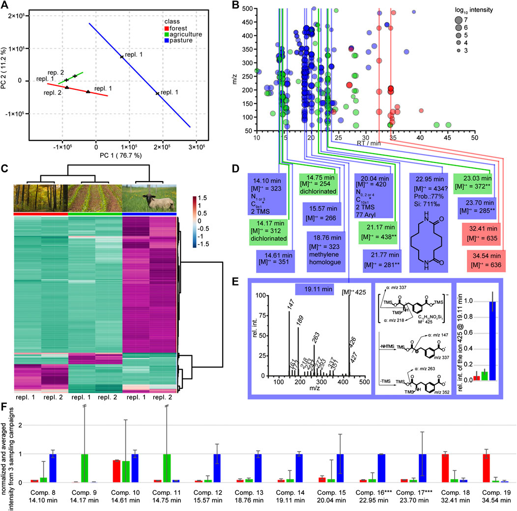
FIGURE 3. Statistical analysis and structure elucidation of seepage water originating from lysimeters of type III. Lysimeters were installed at three different land use sites and data are assigned by red labels for the forest sites, green for the agricultural sites and blue for the pasture sites. (A) PCA score plot of two environmental replicates each for the different land use sites forest, agriculture and pasture based on GC-MS analysis. (B) Heat map of the top 200 (ANOVA) features that contribute to the different land use sites. The dendrograms on top and side of the heat map indicate similarity clusters of the sampling sites and metabolite features, respectively (environmental replicates are numbered). (C) Cloud plot of the top 200 features from the heat map in Figure part B. The color indicates land use and the cloud size the intensity in the mass spectrum. Features that appear at the same retention time are labeled with vertical lines. The most probable chemical identity of these marked feature classes is summarized in part (D). (E) Mass spectrum and suggested fragmentation mechanism of the marker for pasture at 19.11 min (3-caboxyphenylalanine). Including a bar diagram of the relative concentrations (±SD) of the molecular ion 425 occurring in the land use sites. *Carbon number is calculated by the intensity of the [M+1]⁺ ion under consideration of possible silicon isotopes. **Highest observed ion but the low mass is not compatible with the high retention time. (F) Relative intensities of selected compounds (compare Figure part D) monitored in three consecutive sampling campaigns (temporal replication), with environmental duplicate measurements. The graph shows averages (+/− standard deviation) across campaigns per respective land use site, with the highest value per each compound normalized to one. Error bars calculated from the SD by the propagation of error. The compound marked with ** in Figure part D was excluded from the analysis. ***These compounds could only be detected in one of three sampling campaigns (Figure part A–D).

Results and Discussion

Lysimeters

We evaluated three types of lysimeters for their suitability to collect seepage water for the monitoring of organic signatures in soil water using GC-MS. The general aspects (set-up, costs, resistance, chemical artifacts) of the lysimeters are summarized in Table 1, pictures of the lysimeters are given in Figure 2. Lysimeter type I and II were designed for and installed at the topsoil-subsoil boundary thereby allowing the characterization of the input signal that would enter deeper layers. Lysimeter type III was installed to sample seepage water in 30 and 60 cm depth, thereby monitoring water after the passage through the topsoil and additionally the subsoil, respectively. Thus, the water may have estimated dwell time up to one month to undergo transformation until it reaches the sampling device (Sprenger et al., 2016). We aimed for an untargeted qualitative analysis and relative quantification of candidate compounds that allows identifying patterns of variability in water from subsurface environments.

Due to the installation and sampling procedure this set-up gives authentic results regarding the natural flow and water budget.

General Evaluation of the Lysimeters

For the initial evaluation, all three lysimeters were exposed to the environment. We analyzed the soil solution sampled after cumulative collection by the lysimeters. After SPE and desalting with a polymeric amide modified polystyrene resin. GC-MS measurements of the organic eluates were performed after evaporation of the solvent and derivatization with BSTFA, resulting in trimethylsilylation of -OH, -COOH, and -NH₂ groups, following a modified protocol from (Vidoudez and Pohnert, 2012).

It is evident that the three entirely different lysimeter types that also rely on different sampling strategies will give non-uniform patterns of detected compounds. We evaluated if and how environmentally relevant data can be obtained from these different samples and if universal marker compounds can be identified from all three lysimeter set-ups. Visual inspection of the chromatograms revealed substantial qualitative and quantitative differences (Figure 4). Signals caused by plasticizers dominated in chromatograms of type I lysimeter samples. Substantially lower contaminations were detected in type II lysimeter samples. Principal component analysis (PCA, Supplementary Figure S1) confirmed that chemical profiles are highly dependent on sampling instrumentation since the PVC lysimeter (type I) and the inert type II lysimeter showed entirely different profiles despite relying on identical sampling strategies.

FIGURE 4

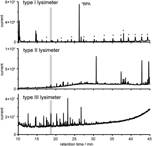
FIGURE 4. Gas chromatography coupled to mass spectrometry (GC-MS) analysis of derivatized water extracts collected by the lysimeters. Gray marked is the internal standard ribitol as penta-TMS derivative. Note, the relative intensities differ in each plot.

The type III lysimeter should not be directly compared with the others since it was installed in deeper soil therefore resulting in long flow path and higher interaction time between soil and seepage. In addition, the sampling was not based on the collection of water by means of gravity but by applying suction in the range of the measured predominant matrix potential, therefore sampling capillary and macropore water. Thus both, the different lysimeter setup and the differences in the chemical composition of the water will be responsible for the major differences in the chemical composition of water sampled with this device. This is clearly illustrated by principal component analysis that show data separated from those obtained with the other lysimeters. However, data are reported here, since inclusion of these samples allows to judge about the suitability and quality of the samples generated.

Especially with lysimeter I we faced several challenges in the further data analysis to reveal the naturally occurring water chemistry composition despite the background signals. Visualization of differences between the samples according to retention time-m/z-pairs of selected analyzed ions, as well as differences in the respective sample types, is given in Supplementary Figure S1A2. The largest difference of any detected signal can be attributed to an m/z value of 357 at 26.2 min in samples obtained from type I lysimeter. The compound was identified as bisphenol A, commonly used in PVC production. All other most dominant signals in this sample can also be attributed to contaminants such as phthalates and fumarates, oxidation stabilizers like butylated hydroxytoluene and decayed stabilizers such as triphenylphosphine oxide (see Supplementary Information). The amount of these contaminations decreased over time when the lysimeter was in use and exposed to environmental conditions (data not shown). Only bisphenol A was found in high amounts over the entire 8-months exposure. As illustrated in detail in the Supplementary Figure S1in silico data treatment like background subtraction leads to data sets of higher quality; however, contaminations could not be entirely suppressed in lysimeters of type I. Strategies for data evaluation that allow targeted and untargeted analysis despite the contaminations are described below.

The type II lysimeter was built from inert material without using any glue or plasticizers and could be used directly after rinsing with bidistilled water without further conditioning. Indeed, we did not detect any of the typical contaminations from e.g., plasticizers or stabilizers under routine sampling conditions. Even if production costs for these lysimeters are comparably high due to the utilized high prized materials, the reduction of contaminations is substantial and a robust data set for qualitative and quantitative analysis can be obtained (Figure 4).

The tension type III lysimeter collected water at greatest depth; this water gave a more than 10-fold lower overall signal intensity compared to those in upper soil (Figure 4). This result is in unison with general observations indicating a depth-dependent reduction of the concentration of total organic carbon and of specific phenolic acids originating mainly from decaying plant material in deeper sampling sites (Martens et al., 2004). The background signal from contaminations is low in lysimeter III, which makes it a good compromise for monitoring fluxes and transformation products in unaffected soils if sampling costs and sample purity is concerned.

Identification of Naturally Occurring Compounds in Lysimeter Samples

Naturally occurring compounds were identified upon visual inspection of the data from samples collected in lysimeters type II and type III. We also subjected the background-corrected file-set from these lysimeters to XCMS data analysis and obtained a cloud plot that allowed identifying common features. Compounds that exhibit sample dependent variability were identified and matched to previously reported naturally occurring compound classes, including carbohydrates (Paul and Clark, 1996), lipids (Jandl et al., 2002) and phenolic acids (Malá et al., 2013). Six of the eight unambiguously identified compounds found in the untargeted analysis using type II and type III lysimeters could also be observed in type I lysimeters in a targeted quantification. This indicates that even the strong contaminants from lysimeter type I do not fully overshadow soil solution chemistry. Among the eight variable compounds were plant or microbe derived α- and β-glucose (RT: 20.20 min) (RT: 22.02 min) that were detected as penta-(trimethylsilyl)-derivatives (supporting information). Glucose cannot be found in chromatograms of samples from the type I lysimeter where it is most likely underdetermined due to adsorption properties of the lysimeter material (Figure 5A). In addition, underdetermination of glucose might also be caused by metabolism in biofilms forming on PVC. Such bacterial activity is suppressed by the use of titanium in the type II lysimeter (Zhang et al., 2014).

FIGURE 5

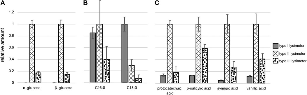
FIGURE 5. Relative amounts of compounds originating from three different types of lysimeters sorted by compound class: (A) sugars, (B) fatty acids, (C) phenolic acids (Note: all compounds were detected as (multiple) tri methyl silyl (TMS)-derivative after N,O-bis(trimethylsilyl)trifluoroacetamide (BSTFA) treatment). Structure identification is based on comparison with authentic standards; normalization was carried out using ribitol as internal standard.

We could also identify saturated fatty acids with a chain length of 16 (palmitic acid) and 18 (stearic acid) carbon atoms as variable marker molecules in the lysimeter extracts. These fatty acids were previously detected in targeted analyzes of soil solutions, and the fact that they are covered with the sampling procedure here, highlights the suitability of the introduced protocols for untargeted screening (Jandl et al., 2002; Jandl et al., 2004; Jandl et al., 2005; Jandl et al., 2007; Schwab et al., 2017). We found the highest abundance of stearic acid in type I lysimeter samples; in comparison, in type II and type III lysimeter samples 3-fold and 12-fold lower amounts were detected, respectively. The differences in palmitic acid concentrations were lower, but again, samples from lysimeters installed close to the surface (type I and II) contained higher amounts compared to those from lysimeter type III at greatest depth (Figure 5B). The fact that saturated fatty acids are more prevalent in samples collected closer to the surface has also been previously observed in targeted analysis of soil extracts (Martens et al., 2004; Schwab et al., 2017).

Four typically occurring phenols, that are connected to humus and lignin chemistry (Schmidt et al., 2011; Lehmann and Kleber, 2015), were also identified using the cloud-plot analysis. Retention time comparison with commercial standards revealed their identity as the phenolic acids protocatechuic acid and p-salicylic acid. Syringic acid and vanillic acid were identified based on the evaluation of their characteristic mass spectra (Malá et al., 2013). The type II lysimeter samples contained the highest amounts of all phenolic acids (Figure 5C). Lower concentrations of these compounds were observed in the type III lysimeter, potentially as a result of transformation, sorption on eg clay minerals or degradation during the passage to greater depth (see Figure 5C). The lowest recovery of these compounds in lysimeters of type I might again be explained by adsorption to PVC. Besides these sugars, fatty acids and phenolic acids, we spotted eight additional common marker compounds. These compounds share a fragment at 131 m/z which might be from Δ^15,7 or Δ^15,8 sterol backbone (Goad and Akihisa, 1997) but could not be fully structurally confirmed (Supplementary Figure S1C2).

Thus, GC-MS-based metabolomics allows a broad survey of biotic and abiotic marker molecules in subsurface solutions. The information-rich EI-MS spectra allow for efficient library search and the chromatographic separation for precise integration. Additional LC-MS studies could be used with the same, underivatized, sample set to complement these data (Supplementary Figure 3). This additional data set covers also larger, more polar metabolites in a complimentary manner. The suitability of the workflow can, however be already judged with the set of GC-MS runs utilized and documented in detail here.

Comparison of the different extracts using the metabolomics workflow shows the strong dependence of profiles on the fabric, functioning, and placement of the lysimeters. This is indicative of a system containing highly diluted compounds that requires careful limitation of interfering signals. Working with devices like type II and type III lysimeters that introduce a minimum of contaminants allows for a straightforward data evaluation. These lysimeters are thus suitable to apply comparative metabolomics algorithms to spot similarities and variation between sites, covering a broad spectrum of natural products. Nevertheless, we show that data obtained with different sampling devices cannot be quantitatively intercompared.

Elucidation of Site-Specific Markers in Seepage Water

With the method evaluation in hands we undertook a survey at three different locations of the Hainich Critical Zone long-term monitoring sites (Küsel et al., 2016). This proof of principle study was undertaken to evaluate the suitability of the approaches for an untargeted survey of soil solution. Due to clear and expected differences of the samples from different lysimeter types, we selected two separate data sets from lysimeters of type I and III and performed two independent data analyzes to identify markers for different land use. Samples were initially analyzed using XCMS (Tautenhahn et al., 2012) and further evaluated by MetaboAnalyst (Xia et al., 2015). We first focused on samples from type I lysimeters installed at three different land use sites (Figure 1). The initial step in our marker identification was the feature recognition including peak picking (of not background subtracted data). The resulting diffreport harbors the vast number of 6,576 total aligned features. To identify markers for the specific sampling site we next processed the data using the online platform MetaboAnalyst 3.0. Filtering, sample specific normalization based on the internal standard ribitol, and Pareto scaling were applied (van den Berg et al., 2006). Ribitol was not contained in unspiked samples (Supplementary Figures 2–5), however in a larger scale screening it would be advised to use labeled standard to fully exclude the potential interference with natural metabolites. In an unsupervised PCA analysis, data showed that 71.6% of the sample variability in the GC/MS data were explained by the first two principal components (PC): PC1, 53.6%; PC2, 18.0%. The forest (red) site clearly separated from the agriculture (green) and the pasture site (blue), which overlap in large areas (Figure 6A). For the identification of marker molecules that are responsible for the separation within the PCA we plotted a heat map, based on the 200 most important features selected by analysis of variance (ANOVA) with a p-value threshold of 0.05. The Euclidean clustering confirmed the separation by the PCA. All three sampling sites can clearly be distinguished (Figure 6B). The forest site shows more specific features than the agricultural site, and only one specific feature could be identified for the pasture site. It is most challenging to translate the detected relevant features into chemical compounds. By means of the features from the ANOVA based heatmap the peak intensities generated by XCMS were used to construct a color-coded cloud plot (Figure 6C). We used the color code to distinguish between the sampling sites and the cloud size to visualize the specific (logarithmic) intensity. Acknowledging that the utilized electron impact ionization produces a series of fragments from a single compound, we combined dominant feature groups and identified one compound specific for the agricultural site, nine for the forest site and none for the pasture site. Three of the compounds had been already annotated in the preliminary lysimeter evaluation (see above): These compounds were p-salicylic acid (comp. 1, 14.87 min), vanillic acid (comp. 3, 17.83 min), and protocatechuic acid (comp. 5, 18.99 min). One further compound was assigned to be a monosaccharide based on typical fragments (m/z = 147 and 117) and the retention time.

FIGURE 6

FIGURE 6. Statistical analysis and structure elucidation of compounds from seepage water collected with lysimeters of type I. Lysimeters were installed at three different land use sites and data are assigned by red labels for the forest sites, green for the agricultural sites and blue for the pasture sites. (A) Principal component analysis (PCA) score plot of six replicates (environmental replicates are numbered, and technical replicates thereof are numbered in brackets) each for the different land use sites based on GC-MS data. (B) Heat map of the top 200 (ANOVA) features that contribute to the different land use sites. The dendrograms on top and side of the heat map indicate similarity clusters of the sampling sites and metabolites, respectively. (C) Cloud plot of the top 200 features from the heat map in Figure part B. The color indicates the respective highest intensity from the sampling sites (by land use) and the cloud-size the signal intensity in the mass spectrum. Features that appear at the same retention time are labeled with vertical lines. The most probable chemical identity of these marked feature classes is summarized in part (D). (E) Relative intensities of compounds from Figure part D. The graph shows averages (+/- standard deviation) across all replicates (environmental and technical) per respective land use site, with the highest value per each compound normalized to one. The compounds labeled with * in Figure part D were excluded from the analysis due to overlapping signals.

Since these markers were gathered from scaled data, we verified the findings by integrating and normalizing the original data (Figure 6E). Despite large standard deviations, most of the relative concentrations were in accordance with their initial assignment to specific land use sites.

A second elucidation of potential marker compounds was based on data gathered using type III lysimeters installed 30 cm below surface. No clear patterns arose from those lysimeters even when testing several scaling techniques like auto scaling or level scaling (van den Berg et al., 2006). In contrast, samples originating from 60 cm depth resulted in clear patterns in unsupervised PCA with respect to the confidence interval. Partial least square discriminant analysis (PLS-DA, not shown) supported the result from the PCA. All three land use sites forest (red), agriculture (green) and pasture (blue) were separated with two principal components (Figure 3A). Two-dimensional PCA summarized 87.9% of the sample variability in the GC-MS data by the first two principal components (PC1, 76.7%; PC2, 11.2%). A heat map was constructed based on the 200 most important features (ANOVA, p value < 0.05). All three sampling sites can clearly be distinguished and the Euclidean clustering (Figure 3B) confirmed the PCA separation. The pasture site shows more specific features than the forest and the agricultural sites (see Figure 3B). The color-coded cloud plot was used to visualize differences between the sampling sites (Figure 3C). Only two compounds which are specific for the forest site are detectable, four compounds were specific for the agricultural and eight for the pasture site. In a NIST library search only the pasture specific feature group at 22.95 min gave a hit with an acceptable probability and spectral identity. The suggested 1,8-diazacyclotetradecane-2,7-dione, a chemical used in nylon 66 production, was assigned as probable artifact or contaminant. Due to the absence of library hits for the other putative markers, structure elucidation on the basis of the reconstructed mass spectra from the XCMS diffreport with further support from the original mass spectral data was conducted. For the forest site, marker structure elucidation was not successful, but compounds like sugars, aliphatic hydrocarbons or fatty acids can be excluded due to missing key fragments. The four agriculture specific markers could not be fully elucidated either, but two of them showed isotopic patterns indicative for two chlorine atoms in the formulae. The exclusive presence of these unknown compounds in the site with heavy land use lets us conclude that they likely represent degradation products of pesticides or related compounds. The elucidation of pasture site related compounds was also challenging and only for the chromatographic peak at 19.11 min we were able to define 3-carboxyphenylalanine as a plausible hit (Supporting information, Figure 3E). This compound was previously isolated from the leaves, stems, roots, and inflorescence of Resedaceae species (Kaa Meier et al., 1979). These belong to the order of Brassicales of which several species exist on our sampling site.

Monitoring of Time Series

The heterogeneity of soil might cause variability of the chemical composition of collected lysimeter water even if instruments are installed in close proximity. To compensate for such influences, we replicated our data in a time series where samples were taken from the same lysimeters (type III) four and six weeks after the above discussed sampling campaign. In addition, we took samples of one additional pasture site within the transect (south western spot in Figure 1). Compounds identified in the untargeted screening (Figure 3D) were monitored in these sampling campaigns. Peaks from each campaign were integrated and normalized (Figure 3F). Indeed, we could track 10 out of 15 putative marker molecules over the three sampling campaigns. All relative concentrations recorded in these independent experiments were in accordance with the findings in Figure 3D. Five compounds could be verified as specific markers for the pasture site (compounds 12 to 14, 16 and 17). Especially the putative 3-carboxyphenylalanine could be proven as marker over the entire monitoring period. Local variability, caused potentially by different histories in agricultural land use, was observed, since the chlorinated compounds two and four were only abundant in one of the two sampling sites.

Conclusion

The lysimeters tested in our analysis are suitable to monitor seepage water chemistry in an untargeted analysis. Cost-minimized PVC based free draining lysimeters enable the installation of several replicates with minimum expenses. However, initial bleeding leads to signals of contaminants that are dominant compared to the natural products and require for extensive data treatment. The newly designed PEEK/titanium lysimeter, as well as tension lysimeters made from stainless steel/inert glass, allowed for seepage collection of samples that give high-quality chromatographic profiles. With some limitations of the PVC instruments, all lysimeters enable to analytically follow a structurally diverse series of compound classes as we have shown for sugars, fatty acids, phenolic acids. Sample heterogeneity is generally lower in deeper soil. Here not further discussed, but illustrated in Supplementary Figure 6, the SPE eluates and thus the whole sample pre-treatment is also suitable for LC-MS based metabolomic methods which broadens the field of application from this study.

An untargeted data evaluation of lysimeter solutions allowed the identification of land use markers. Three phenolic acids can serve as specific markers for the forest land use site with lysimeters of type I. Additional markers for the land use forest (2), pasture (9), and agriculture (4) were identified. Two not further specified chlorinated compounds served as markers for the agricultural site in 60 cm depth, the putative 3-carboxyphenylalanine as a marker to the pasture site. Ten out of these 15 site-specific markers could also be traced over time in two additional sampling campaigns. Thus, GC-MS-based untargeted seepage analysis allows to identify a broad range of markers that can be used for the identification of spatiotemporal cycling patterns and for the tracing of matter fluxes within subsurface compartments of the Critical Zone.

Data Availability Statement

The raw data supporting the conclusion of this article will be made available by the authors, without undue reservation.

Author Contributions

NU performed metabolomics analysis and implemented lysimeter type II. KL, AS, and SM maintained the Lysimeters type I and III implemented and KT, BM, and GP contributed to the conception and design of the work. NU, CZ and GP wrote the manuscript. All authors contributed to the final version of the manuscript.

Conflict of Interest

The authors declare that the research was conducted in the absence of any commercial or financial relationships that could be construed as a potential conflict of interest.

Acknowledgments

The authors acknowledge the DFG for funding within theframework of the SFB 1076 ‘‘AquaDiva” under project number 218627073. Field work permits were issued by the responsible state environmental offices of Thuringia, Germany. We thank the Hainich CZE site manager Robert Lehmann, Christine Hess and Maria Fabisch for scientific coordination, Bernd Ruppe for field sampling, and the Hainich National Park administration.

Supplementary Material

The Supplementary Material for this article can be found online at: https://www.frontiersin.org/articles/10.3389/feart.2020.563379/full#supplementary-material.

References

Alonso, A., Marsal, S., and Julià, A. (2015). Analytical methods in untargeted metabolomics: state of the art in 2015. Front. Bioeng. Biotechnol. 3, 23. doi:10.3389/fbioe.2015.00023

PubMed Abstract | CrossRef Full Text | Google Scholar

Bianchi, T. S., and Canuel, E. A. (2011). Chemical biomarkers in aquatic ecosystems. Princeton, NJ: Princeton University Press.

Google Scholar

Brock, O., Kalbitz, K., Absalah, S., and Jansen, B. (2020). Effects of development stage on organic matter transformation in Podzols. Geoderma. 378, 114625. doi:10.1016/j.geoderma.2020.114625

CrossRef Full Text | Google Scholar

Brown, S. C., Kruppa, G., and Dasseux, J. L. (2005). Metabolomics applications of FT-ICR mass spectrometry. Mass Spectrom. Rev. 24 (2), 223–231. doi:10.1002/mas.20011

PubMed Abstract | CrossRef Full Text | Google Scholar

Bundy, J. G., Davey, M. P., and Viant, M. R. (2009). Environmental metabolomics: a critical review and future perspectives. Metabolomics 5 (1), 3–21. doi:10.1007/s11306-008-0152-0

CrossRef Full Text | Google Scholar

Dibbern, D., Schmalwasser, A., Lueders, T., and Totsche, K. U. (2014). Selective transport of plant root-associated bacterial populations in agricultural soils upon snowmelt. Soil Biol. Biochem. 69, 187–196. doi:10.1016/j.soilbio.2013.10.040

CrossRef Full Text | Google Scholar

Fenoll, J., Hellín, P., Martínez, C. M., Flores, P., and Navarro, S. (2011). Determination of 48 pesticides and their main metabolites in water samples by employing sonication and liquid chromatography-tandem mass spectrometry. Talanta. 85 (2), 975–982. doi:10.1016/j.talanta.2011.05.012

PubMed Abstract | CrossRef Full Text | Google Scholar

Fischer, K., Wacht, M., and Meyer, A. (2003). Simultaneous and sensitive HPLC determination of mono- and disaccharides, uronic acids, and amino sugars after derivatization by reductive amination. Acta Hydrochim. Hydrobiol. 31 (2), 134–144. doi:10.1002/aheh.200300484

CrossRef Full Text | Google Scholar

Freeze, R. A. (1969). The mechanism of natural ground-water recharge and discharge: 1. One-dimensional, vertical, unsteady, unsaturated flow above a recharging or discharging ground-water flow system. Water Resour. Res. 5 (1), 153–171. doi:10.1029/WR005i001p00153

CrossRef Full Text | Google Scholar

Frimmel, F. H., Abbt-Braun, G., Heumann, K. G., Hock, B., Lüdemann, H.-D., and Spiteller, M. (2002). Refractory organic substances in the environment. Weinheim, Germany: WileyVCH.

Google Scholar

García-Sevillano, M. Á., García-Barrera, T., and Gómez-Ariza, J. L. (2015). Environmental metabolomics: biological markers for metal toxicity. Electrophoresis 36 (18), 2348–2365. doi:10.1002/elps.201500052

PubMed Abstract | CrossRef Full Text | Google Scholar

Goad, L. J., and Akihisa, T. (1997). Analysis of sterols. Blackie Academic & Professional.

Google Scholar

Haarstad, K., Bavor, H. J., and Mæhlum, T. (2012). Organic and metallic pollutants in water treatment and natural wetlands: a review. Water Sci. Technol. 65 (1), 76–99. doi:10.2166/wst.2011.831

PubMed Abstract | CrossRef Full Text | Google Scholar

Jandl, G., Leinweber, P., Schulten, H. R., and Ekschmitt, K. (2005). Contribution of primary organic matter to the fatty acid pool in agricultural soils. Soil Biol. Biochem. 37 (6), 1033–1041. doi:10.1016/j.soilbio.2004.10.018

CrossRef Full Text | Google Scholar

Jandl, G., Leinweber, P., Schulten, H. R., and Eusterhues, K. (2004). The concentrations of fatty acids in organo-mineral particle-size fractions of a Chernozem. Eur. J. Soil Sci. 55 (3), 459–469. doi:10.1111/j.1365-2389.2004.00623.x

CrossRef Full Text | Google Scholar

Jandl, G., Leinweber, P., and Schulten, H. R. (2007). Origin and fate of soil lipids in a Phaeozem under rye and maize monoculture in Central Germany. Biol. Fertil. Soils 43 (3), 321–332. doi:10.1007/s00374-006-0109-2

CrossRef Full Text | Google Scholar

Jandl, G., Schulten, H.-R., and Leinweber, P. (2002). Quantification of long-chain fatty acids in dissolved organic matter and soils. J. Plant Nutr. Soil Sci. 165. 2-T, 133–139. doi:10.1002/1522-2624

CrossRef Full Text | Google Scholar

Kaa Meier, L., Olsen, O., and Sorensen, H. (1979). Acidic amino acids in Reseda luteola. Phytochem. 18 (9), 1505–1509. doi:10.1016/S0031-9422(00)98484-X

CrossRef Full Text | Google Scholar

Kohlhepp, B., Lehmann, R., Seeber, P., Küsel, K., Trumbore, S. E., and Totsche, K. U. (2017). Aquifer configuration and geostructural links control the groundwater quality in thin-bedded carbonate–siliciclastic alternations of the Hainich CZE, central Germany. Hydrol. Earth Syst. Sci. 21 (12), 6091–6116. doi:10.5194/hess-21-6091-2017

CrossRef Full Text | Google Scholar

Kramer, S., Marhan, S., Ruess, L., Armbruster, W., Butenschoen, O., Haslwimmer, H., et al. (2012). Carbon flow into microbial and fungal biomass as a basis for the belowground food web of agroecosystem. Pedobio. 55 (2), 111–119. doi:10.1016/j.pedobi.2011.12.001

CrossRef Full Text | Google Scholar

Kuhlisch, C., and Pohnert, G. (2015). Metabolomics in chemical ecology. Nat. Prod. Rep. 32 (7), 937–955. doi:10.1039/c5np00003c

PubMed Abstract | CrossRef Full Text | Google Scholar

Küsel, K., Totsche, K. U., Trumbore, S. E., Lehmann, R., Steinhäuser, C., and Herrmann, M. (2016). How deep can surface signals be traced in the critical zone? Merging biodiversity with biogeochemistry research in a central German Muschelkalk landscape. Front. Earth Sci. 4. doi:10.3389/feart.2016.00032

CrossRef Full Text | Google Scholar

Lehmann, J., and Kleber, M. (2015). The contentious nature of soil organic matter. Nature. 528 (7580), 60–68. doi:10.1038/nature16069

PubMed Abstract | CrossRef Full Text | Google Scholar

Lehmann, K., Lehmann, R., and Totsche, K. U. (2020). Event-driven dynamics of the total mobile inventory in undisturbed soil account for significant fluxes of particulate organic carbon. Sci. Total Environ. 143774. doi:10.1016/j.scitotenv.2020.143774

PubMed Abstract | CrossRef Full Text | Google Scholar

Leyva, D., Jaffe, R., and Fernandez-Lima, F. (2020). Structural characterization of dissolved organic matter at the chemical formula level using TIMS-FT-ICR MS/MS. Anal. Chem. 92 (17), 11960–11966. doi:10.1021/acs.analchem.0c02347

PubMed Abstract | CrossRef Full Text | Google Scholar

Lloyd, C. E. M., Michaelides, K., Chadwick, D. R., Dungait, J. A. J., and Evershed, R. P. (2012). Tracing the flow-driven vertical transport of livestock-derived organic matter through soil using biomarkers. Org. Geochem. 43, 56–66. doi:10.1016/j.orggeochem.2011.11.001

CrossRef Full Text | Google Scholar

Malá, J., Cvikrová, M., Hrubcová, M., and Máchová, P. (2013). Influence of vegetation on phenolic acid contents in soil. J. For. Sci. 59 (7), 288–294. doi:10.17221/23/2013-JFS

CrossRef Full Text | Google Scholar

Martens, D. A., Reedy, T. E., and Lewis, D. T. (2004). Soil organic carbon content and composition of 130-year crop, pasture and forest land-use managements. Global Change Biol. 10 (1), 65–78. doi:10.1046/j.1529-8817.2003.00722.x

CrossRef Full Text | Google Scholar

Medeiros, P. M., and Simoneit, B. R. (2007). Analysis of sugars in environmental samples by gas chromatography-mass spectrometry. J. Chromatogr. A. 1141 (2), 271–278. doi:10.1016/j.chroma.2006.12.017

PubMed Abstract | CrossRef Full Text | Google Scholar

Olofsson, M. A., Norström, S. H., and Bylund, D. (2014). Evaluation of sampling and sample preparation procedures for the determination of aromatic acids and their distribution in a podzol soil using liquid chromatography–tandem mass spectrometry. Geoderma. 232–234, 373–380. doi:10.1016/j.geoderma.2014.06.005

PubMed Abstract | CrossRef Full Text | Google Scholar

Paul, A., and Clark, F. E. (1996). Soil Microbiology and Biochemistry. Cambridge, MA: Academic Press.

Google Scholar

Winton, K., and Weber, J. B. (1996). A review of field lysimeter studies to describe the environmental fate of pesticides. Weed Technol. 10 (1), 202–209. doi:10.1017/S0890037X00045929

CrossRef Full Text | Google Scholar

Robertson, G. P., Kellogg, W. K., Coleman, D. C., Bledsoe, S., and Sollins, P. (1999). Standard soil methods for long-term ecological research. Oxford, England: Oxford University Press.

Google Scholar

Roth, V. N., Dittmar, T., Gaupp, R., and Gleixner, G. (2015). The molecular composition of dissolved organic matter in forest soils as a function of pH and temperature. PloS One 10 (3), e0119188. doi:10.1371/journal.pone.0119188

PubMed Abstract | CrossRef Full Text | Google Scholar

Schmidt, M. W., Torn, M. S., Abiven, S., Dittmar, T., Guggenberger, G., Janssens, I. A., et al. (2011). Persistence of soil organic matter as an ecosystem property. Nature 478 (7367), 49–56. doi:10.1038/nature10386

PubMed Abstract | CrossRef Full Text | Google Scholar

Siemens, J., and Kaupenjohann, M. (2004). Comparison of three methods for field measurement of solute leaching in a sandy soil. Soil Sci. Soc. Am. J. 68 (4), 1191–1196. doi:10.2136/sssaj2004.1191

CrossRef Full Text | Google Scholar

Siemens, J., and Kaupenjohann, M. (2003). Dissolved organic carbon is released from sealings and glues of pore-water samplers. Soil Sci. Soc. Am. J. 67 (3), 795–797. doi:10.2136/sssaj2003.7950

CrossRef Full Text | Google Scholar

Singh, G., Kaur, G., Williard, K., Schoonover, J., and Kang, J. (2018). Monitoring of water and solute transport in the vadose zone: a review. Vadose Zone J. 17 (1), 160058. doi:10.2136/vzj2016.07.0058

CrossRef Full Text | Google Scholar

Sprenger, M., Seeger, S., Blume, T., and Weiler, M. (2016). Travel times in the vadose zone: variability in space and time. Water Resour. Res. 52 (8), 5727–5754. doi:10.1002/2015WR018077

CrossRef Full Text | Google Scholar

Sysi-Aho, M., Katajamaa, M., Yetukuri, L., and Oresic, M. (2007). Normalization method for metabolomics data using optimal selection of multiple internal standards. BMC Bioinf. 8, 93. doi:10.1186/1471-2105-8-93

CrossRef Full Text | Google Scholar

Tautenhahn, R., Patti, G. J., Rinehart, D., and Siuzdak, G. (2012). XCMS Online: a web-based platform to process untargeted metabolomic data. Anal. Chem. 84 (11), 5035–5039. doi:10.1021/ac300698c

PubMed Abstract | CrossRef Full Text | Google Scholar

Thieme, L., Graeber, D., Hofmann, D., Bischoff, S., Schwarz, M. T., Steffen, B., et al. (2019). Dissolved organic matter characteristics of deciduous and coniferous forests with variable management: different at the source, aligned in the soil. Biogeosci. 16 (7), 1411–1432. doi:10.5194/bg-16-1411-2019

CrossRef Full Text | Google Scholar

Totsche, K. U., Jann, S., and Kögel-Knabner, I. (2007). Single event–driven export of polycyclic aromatic hydrocarbons and suspended matter from coal tar–contaminated soil. Vadose Zone J. 6 (2), 233–243. doi:10.2136/vzj2006.0083

CrossRef Full Text | Google Scholar

Trumbore, V. F., Herrmann, M., Roth, V. N., Gleixner, G., Lehmann, R., Pohnert, G., et al. (2017). Functional diversity of microbial communities in pristine aquifers inferred by PLFA- and sequencing-based approaches. Biogeosci. 14 (10), 2697–2714. doi:10.5194/bg-14-2697-2017

CrossRef Full Text | Google Scholar

van den Berg, R. A., Hoefsloot, H. C., Westerhuis, J. A., Smilde, A. K., and van der Werf, M. J. (2006). Centering, scaling, and transformations: improving the biological information content of metabolomics data. BMC Genom. 7 (1), 142–215. doi:10.1186/1471-2164-7-142

CrossRef Full Text | Google Scholar

Vidoudez, C., and Pohnert, G. (2012). Comparative metabolomics of the diatom Skeletonema marinoi in different growth phases. Metabolomics 8 (4), 654–669. doi:10.1007/s11306-011-0356-6

CrossRef Full Text | Google Scholar

Weihermüller, L., Siemens, J., Deurer, M., Knoblauch, S., Rupp, H., Göttlein, A., et al. (2007). In situ soil water extraction: a review. J. Environ. Qual. 36 (6), 1735–1748. doi:10.2134/jeq2007.0218

PubMed Abstract | CrossRef Full Text | Google Scholar

Withers, E., Hill, P. W., Chadwick, D. R., and Jones, D. L. (2020). Use of untargeted metabolomics for assessing soil quality and microbial function. Soil Biol. Biochem. 143, 107758. doi:10.1016/j.soilbio.2020.107758

CrossRef Full Text | Google Scholar

Xia, J., Sinelnikov, I. V., Han, B., and Wishart, D. S. (2015). MetaboAnalyst 3.0—making metabolomics more meaningful. Nucleic Acids Res. 43 (W1), W251–W257. doi:10.1093/nar/gkv380

PubMed Abstract | CrossRef Full Text | Google Scholar

Ye, Q., Wang, Y.-H., Zhang, Z.-T., Huang, W.-L., Li, L.-P., Li, J., et al. (2020). Dissolved organic matter characteristics in soils of tropical legume and non-legume tree plantations. Soil Biol. Biochem. 148, 107880. doi:10.1016/j.soilbio.2020.107880

CrossRef Full Text | Google Scholar

Zhang, L., Lehmann, K., Totsche, K. U., and Lueders, T. (2018). Selective successional transport of bacterial populations from rooted agricultural topsoil to deeper layers upon extreme precipitation events. Soil Biol. Biochem. 124, 168–178. doi:10.1016/j.soilbio.2018.06.012

CrossRef Full Text | Google Scholar

Zhang, W. P., Wang, Y., Tian, R. M., Bougouffa, S., Yang, B., and Cao, H. L., (2014). Species sorting during biofilm assembly by artificial substrates deployed in a cold seep system. Sci. Rep. 4, 6647. doi:10.1038/srep06647

PubMed Abstract | CrossRef Full Text | Google Scholar