Pathways for Methane Emissions and Oxidation that Influence the Net Carbon Balance of a Subtropical Cypress Swamp

Introduction

Inland aquatic ecosystems actively cycle carbon from the terrestrial biosphere (Battin et al., 2009), which results in large emissions of greenhouse gases (GHGs) such as carbon dioxide (CO₂) (Raymond et al., 2013; Sawakuchi et al., 2017) and methane (CH₄) (Baker-Blocker et al., 1977; Matthews and Fung, 1987) from inland waters to the atmosphere. Wetlands play a prominent role in the inland water carbon cycle due to their close connection between water, vegetation, and land. High rates of primary production by terrestrial and aquatic vegetation and low redox potential conditions in wetlands favor both organic carbon (OC) burial and methanogenesis, the relative balance of which regulate wetland impacts on the atmospheric GHG balance (Mitsch and Gosselink, 2007). Wetlands are the largest natural source of methane to the atmosphere with a global flux of 55–231 Tg C yr⁻¹ (Houweling et al., 2000; Wuebbles and Hayhoe, 2002; Neef et al., 2010). The balance between carbon burial and GHG emissions in wetlands and aquatic ecosystems along the land-ocean continuum remain poorly constrained in the global carbon cycle and poorly represented in Earth system models (Ward et al., 2017; Ward et al., 2020).

The role of CH₄ in this balance is particularly difficult and important to constrain because of high spatiotemporal variability in field observations and high global warming potential compared to CO₂; CH₄ has 96 and 11 times the warming potential of CO₂ when CH₄ emissions are sustained for 20 and 500 years, respectively (Neubauer and Megonigal, 2015). An evaluation of three wetlands ecosystems along a latitudinal gradient showed that the molar ratio of CH₄ emitted to net atmospheric CO₂ fixation by vegetation on an annual basis ranged from 0.05 to 0.20 (Whiting and Chanton, 2001). Considering the relative global warming potential of CH₄, these wetlands exacerbate atmospheric greenhouse effect over short (20 years) time scales, but serve as net sinks of warming potential (i.e., produce a global cooling effect) over 100–500 years timescales since the atmospheric residence time of methane is an order of magnitude shorter than CO₂ (Whiting and Chanton, 2001).

Global estimates of CH₄ emissions from wetlands are poorly constrained because complex interactions between hydrology, vegetation, and soil/sediment properties result in emissions that can be orders of magnitude different even at short separation distances (Bridgman et al., 2013). Gaps in mechanistic understanding of how methane is produced, consumed, and emitted from wetlands further complicate predictions for how these ecosystems will respond to future climate and restoration scenarios (Riley et al., 2011). Fluctuating water table dynamics in wetlands means that saturated, inundated, and aerated zones exist and shift over time, with implications for where and when CH₄ is produced. However, general predictions about these dynamic controls on CH₄ emissions remains unclear because the functional relationship between water table height and CH₄ emissions is inconsistent across studies and wetland types. For example, CH₄ emissions respond differently to water table height in bogs, fens, and swamps while antecedent conditions (e.g., dry periods) appear to exert an important influence (Turetsky et al., 2014).

Wetland vegetation plays an important role in transporting CH₄ from belowground to the atmosphere because the soil and porewater that are the venue for plant roots contain high CH₄ levels (Schutz, 1991), and because vascular plant tissues are known to offer reduced resistance to atmospheric gas exchange. This phenomenon has been well-studied in herbaceous plants (Nouchi et al., 1990; Nisbet et al., 2009), but woody plants have recently been recognized as also playing an important role in transporting CH₄ to the atmosphere both in wetlands and upland forests (Barba et al., 2019a). In tropical wetlands, for example, emissions from tree stems accounted for up to 65% of total ecosystem CH₄ emissions (Pangala et al., 2017).

Despite the clear role of plant vascular systems in gas transport, few studies have considered some of the unique morphological features of highly flood tolerant trees. For example, flood tolerant trees of the genus Taxodium have “cypress knees” that visually appear similar to pneumatophores found in mangroves. However, the function of cypress knees remains unknown. Despite the ability for Taxodium to thrive in low oxygen soil environments compared to other genera (Pezeshki et al., 1996; Anderson and Pezeshki, 2000) there is little evidence that their emergent root structures provide oxygen to the root system. Another proposed function is that the knees provide stability in soft muddy soil (Briand, 2000). Considering these emergent structures provide a direct link between the anaerobic subsurface and the atmosphere, they may be an active, but largely unknown pathway for CH₄ emissions. Several studies have measured CH₄ flux rates from cypress knees, registering significantly higher evasion rates than nearby surface waters and soils (Pulliam, 1992; Bianchi et al., 1996). Likewise, pneumatophores have been shown to be conduits for methane emissions in mangrove forests (Purvaja et al., 2004). An experimental study showed that methane emissions from Taxodium distichum trees increased under both elevated ambient CO₂ levels and water table depth, suggesting that wetland methane emissions will increase under future climate scenarios (Vann and Megonigal, 2003). Despite their ubiquity in many coastal plain swamps, it remains unclear how important knees are for overall CH₄ emissions, particularly since this pathway would bypass microbial processes that might otherwise reduce methane export.

The microbial oxidation of methane (MOX) has been shown to dramatically reduce emissions from surface water environments such as rivers, in some cases by ∼99% (Sawakuchi et al., 2016). The magnitude and mechanisms for MOX, however, remain poorly constrained and are not frequently measured alongside emissions (Segers, 1998). Aerated surface waters are the most likely venue for MOX to occur, but MOX has also been attributed to processes occurring within herbaceous plants (Frenzel and Rudolph, 1998; Frenzel, 2000). If wetland surface waters play an important role in reducing CH₄ emissions similar to rivers and lakes (Bastviken et al., 2002), then emissions from vegetation may represent an important pathway to “bypass” this oxidative layer. A similar phenomenon has been observed in brackish coastal floodplains, where transpiration by trees allowed CH₄ produced deep in the soil profile (below shallow layers where sulfate inhibits methanogenesis) to bypass oxidation in the shallow soil layers (Ward et al., 2019).

Small aquatic ecosystems such as ponds and wetlands are increasingly recognized as exerting outsized influence on global aquatic GHG emissions (Holgerson and Raymond, 2016; DelSontro et al., 2018; Peacock et al., 2019), but settings with extensive organic matter turnover, such as cypress dome wetlands, remain poorly studied (Villa and Mitsch, 2014; Pereyra and Mitsch, 2018). Here, we examine methane cycling and carbon burial dynamics in the Big Cypress National Preserve (BICY) in southwest Florida, a subtropical wetland characterized by isolated forest wetland depressions (cypress domes) that are evenly distributed within short-hydroperiod marshes and pine uplands (Watts et al., 2014). The cypress domes in BICY are thought to form via feedback between water storage and carbonate rock dissolution, mediated and accelerated by organic matter cycling (Cohen et al., 2011; Dong et al., 2019). The resulting regular pattern of wetland sizes and arrangement (Quintero and Cohen, 2019) illustrates the importance of these feedbacks in creating geomorphic structure, a process thought to have occurred over the last 10,000 years (Chamberlin et al., 2018; Zhang et al., 2019).

Given the central importance of carbon cycling to the evolution of landscape depressions, our overarching goal was to enumerate carbon fluxes in these wetlands. The central relevance of methane fluxes in BICY emerges from a global understanding that wetlands are important control points for land-atmosphere methane exchanges, and from the local need to understand the hydrologic controls on organic matter cycling. Our objective was to quantify the components of CH₄ losses from small seasonal wetlands and evaluate how carbon burial balances with these CH4 flux pathways over 20–500 yr timescales. This required us to quantify the mass fluxes of methane in saturated and inundated settings, with varying water table conditions, to enumerate the mass fluxes through emergent root structures, and also to quantify mass retention due to water column oxidation. Measured methane emissions and existing carbon burial data (Zhang et al., 2019) was then scaled across the wetlands to evaluate the net radiative balance of the system. We hypothesized that the presence of oxic surface waters reduces overall wetland emissions, while emissions from cypress knees and ebullition bypass MOX and contribute significantly to wetland-scale emissions. We further hypothesized that the combination of these methane flux pathways will result in the system being a net source of atmospheric warming over decadal timescales.

Materials and Methods

Study Site

The Big Cypress National Preserve is a flat (mean surface slope = 0.03 m km⁻¹) karst landscape in southwestern Florida, and part of the Greater Everglades ecosystem (Figures 1A–C). The combination of low relief and a humid subtropical climate with mean annual precipitation of 1.33 m (McPherson, 1974; Shoemaker et al., 2011) results in significant water storage on the landscape. Thousands of small (< 2 ha) karst depressions dot the landscape in a remarkable regularly patterned landscape of distributed water storage (Quintero and Cohen, 2019). These depressions have far thicker soils (Watts et al., 2014) with far higher OC content (Zhang et al., 2019) than the surrounding uplands because they hold water for much of the year, thereby supporting hydrophytic vegetation such as pond cypress (Taxodium ascendens) and a variety of wetland taxa (e.g., Salix caroliniana, Cladium jamaicense). These cypress “domes,” so called because the cypress trees at the margins are typically shorter than those in the center due to growth rate differences (Katherine, 1988), are crucial elements in the complex mosaic that makes BICY an important biodiversity hotspot. The mosaic of uplands within which these depressions occur are dominated by cabbage palm (Sabal palmetto) and south Florida slash pine (Pinus elliottii var. densa) and, in stark contrast to the wetlands, are rarely inundated and lack any soil development.

FIGURE 1

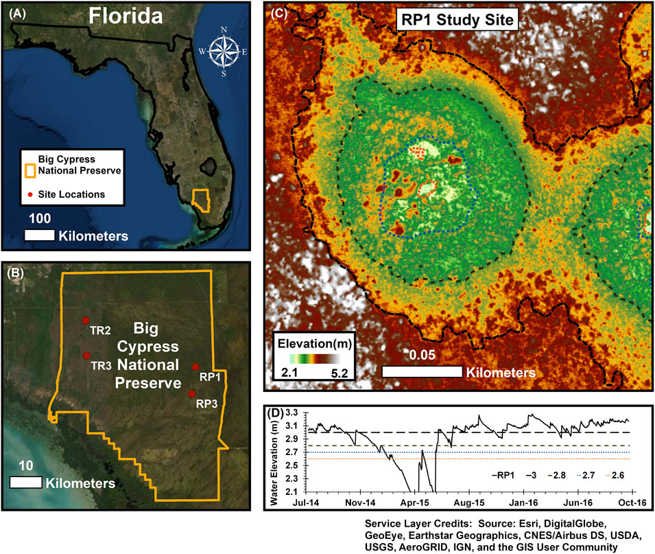
FIGURE 1. (A,B) Measurements were made at four wetlands in the Big Cypress National Preserve. (C) Wetlands are described as cypress domes with three distinct elevation zones that we defined as the center, intermediate, and edge zones. (D) Water elevation was below the ground surface for many of the wetlands and their three zones during the dry season, while the intermediate and center zones were inundated for the majority of the year (see Table 3).

Water levels in the wetlands follow pronounced seasonal patterns in rainfall and evapotranspiration; high water levels typically occur in the summer and fall, with drydown over the winter and the lowest water levels in late spring (Figure 1D). Hydrologic connectivity in this landscape occurs when the wetlands fill sufficiently to exceed a critical stage threshold where water spills out and generates landscape sheetflow (McLaughlin et al., 2019); below this spill threshold, wetlands hold water but do not appear to exchange water regionally. While construction of elevated roads and canals for logging, oil drilling, and recreation over the last century has resulted in localized hydrologic modification (McPherson, 1974), the hydrologic and biological conditions in BICY are far less impacted than in the adjacent Everglades system.

We studied four cypress domes across two contrasting lithologies within BICY. Two were in the region known as Raccoon Point, near the end of 11-Mile Road (RP1: 25.9896 N, 80.9279 W and RP3: 25.9144 N, 80.9392 W) on the Pleistocene Fort Thompson Formation, a more recent carbonate lithology with a high proportion of insoluble material. The RP domes were shallower, and lacked surface water during the dry season. The other two domes were located near Turner River Road (TR2: 26.1197 N, 81.2691 W, and TR3: 26.0208 N, 81.2661 W), located on the Miocene Tamiami Formation. The TR domes were deeper, and each wetland center was inundated during the entire study period. All sampling described below was performed during daylight hours, generally between 10:00 and 15:00.

Above and Belowground CH₄ Concentrations and Stable Isotopic Composition

The partial pressure of CH₄ (pCH₄) and stable isotopic composition (δ¹³C-CH₄) was measured in surface waters, bubbles collected from the sediment-water interface, and two porewater depths at three locations per wetland site—the edge of the wetland near the upland-wetland boundary, midway into the wetland, and the center of the wetland (Figure 1C and Figure 2). For each of these locations, nested porewater samplers were installed to the soil-bedrock interface and a depth halfway between the bedrock and sediment-water interface (Table 1). The samplers were constructed of 5.1 cm diameter schedule 80 PVC and had 10 cm long sections with 125 µm well screening at their base. Water was pumped from each sampler through an overflow cup which contained calibrated (daily) YSI ProPlus pH, DO, specific conductivity, and temperature probes. Water was pumped until all parameters stabilized, to ensure pristine porewaters were sampled.

FIGURE 2

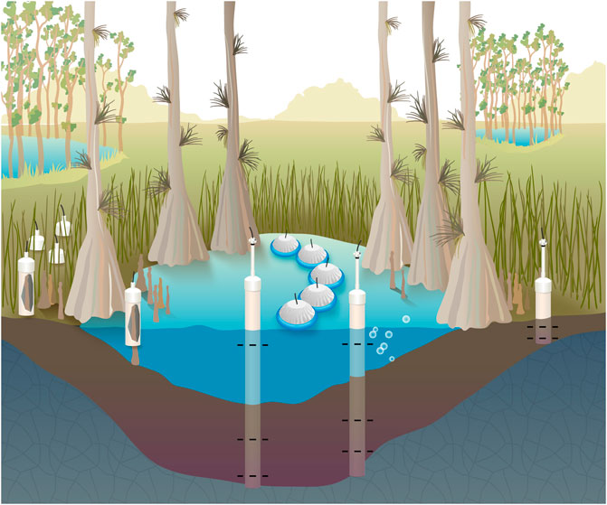
FIGURE 2. The concentration and stable isotopic composition of methane was measured in surface waters, porewaters sampled near the bedrock interface and midway between the bedrock and sediment surface, and bubbles extracted from sediments. Methane fluxes were measured from surface waters, non-inundated soils when present, and cypress tree knees. These measurements were made in the center of the domes, the edge of the dome, and a midpoint between these locations.

TABLE 1

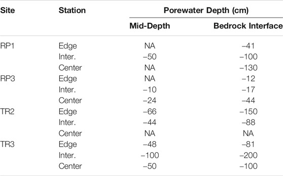
TABLE 1. Depth belowground for porewater sampling at each wetland edge, intermediate point (Inter.), and wetland center sampling stations. NA indicates depths that were not sampled due to logistical constraints.

Sampling for measurements of pCH₄ and δ¹³C-CH₄ values included overfilling 635 ml polycarbonate bottles for about three bottle volumes ensuring they contained no bubbles. The bottles were closed with butyl stoppers equipped with two stop-cocks and short/long straws to allow creation of a headspace by removing 60 ml of water and injecting 60 ml of N₂ to fill the headspace without contact with the atmosphere (Ward et al., 2016). The bottle was shaken vigorously for 2 min and the headspace was extracted into a 60 ml syringe.

After collecting the above samples and measuring CH₄ fluxes (described below), bubbles were collected from the sediment-water interface to measure non-microbially degraded δ¹³C-CH₄ values. Bubbles were collected by manually disturbing the sediment and capturing the released gas in an inverted funnel equipped with a 3-way luer valve (Sawakuchi et al., 2016). When the funnel filled with sediment bubbles, the gas was collected in 60 ml syringes. Prior to collecting the bubbles, care was taken to not disturb sediments as porewater were collected and flux measurements were made. δ¹³C-CH₄ data from the bubbles was used in our estimations of MOX (Estimations of CH₄Oxidation).

Gas samples were injected from the syringe into a Picarro G2201-i Cavity Ring-Down Spectrometer (CRDS) within ∼12 h of sampling to measure pCH₄ and δ¹³C-CH₄. Porewater and bubble samples were diluted 10–1,000 times with pure N₂ prior to analysis to achieve values within the CRDS’s detection range. pCH₄ values were corrected for dilution with N₂ based on the common gas law. pCH₄ values are reported in ppt units considering the high values recorded in porewaters and bubbles.

CH₄ fluxes From Surface Water, Soils, and Cypress Knees

The flux of CH₄ was measured using various opaque chambers depending on the source of the CH₄ flux (Figure 2). For surface waters we used a “floating dome” design, which was an inverted high density polyethelene planter pot with polyethelene foam glued to its rim for flotation (Sawakuchi et al., 2017). The chamber was wrapped in tin foil to avoid heating of the headspace, which was sampled via an air-tight 2-way luer valve. The surface water chambers had a volume of 9.9 L, diameter of 0.33 m where the chamber meets the water, and surface area of 0.086 m² where the chamber meets the water. Five replicate chambers were deployed simultaneously for 5–6 min, after which the headspace was sampled using a 60 ml syringe. Ambient air was also sampled in the same manner.

When surface waters were not present, e.g., at the edge of the wetland during certain sampling periods, we utilized triplicate soil flux chambers constructed from white PVC pipe with a sealed endcap on one end and air-tight 2-way luer valve. Chambers were gently placed on the soil surface for 4–5 min and samples were collected in 60 ml syringes. The soil chambers had a volume of 2.0 L, diameter of 0.10 m where the chamber meets the soil, and a surface area of 0.008 m² where the chamber meets the soil.

Another chamber, made out of the same PVC materials used for the soil chambers, was designed to fit over cypress knees protruding from the water surface (Figure 2). At inundated sampling stations the chamber’s opening was placed just below the water surface so as to not touch the sediment-water interface for 5 min prior to sampling with a 60 ml syringe. One chamber was deployed in triplicate over one knee per sampling location when present; no cypress trees or knees were present at TR3. In order to calculate how much of the chamber’s volume was submerged under water and filled with the knee above the water-air interface, we measured how deep the chamber was submerged underwater, the knee height above the water surface, and the circumference at the bottom and top of the knee assuming the geometry of a tapered cylinder.

For each chamber design, a Licor-820 with external diaphragm pump was interfaced to one chamber to monitor CO₂ fluxes (not reported here) and to ensure that the chamber’s headspace was initially in equilibrium with the atmosphere and did not reach equilibrium with the surface waters/soils/knees during the deployment (i.e. gas fluxes remained linear). Water and air temperatures were measured using a YSI Pro Plus multiparameter sonde. Samples collected from the flux chambers were analyzed by direct injection on the CRDS as previously described. The rate of change ($\frac{dC{H}_4}{dt}$; atm L⁻¹ min⁻¹) was calculated as follows:

$\frac{dC{H}_4}{dt}=\frac{pC{H}_4^f - pC{H}_4^i}{t} (1)$

where $pC{H}_4^f$ is the partial pressure of CH₄ inside the flux chamber at the end of the deployment (atm L⁻¹), $pC{H}_4^i$ is the partial pressure of CH₄ in ambient air collected with a syringe (atm L⁻¹), and t is the length of time between placing the chamber on the water, soil, or knee and sampling the chamber’s headspace (minutes). CH₄ fluxes (F_CH4; μmol m⁻² min⁻¹) were then calculated based on the ideal gas law as follows:

${\text{F}}_{\text{CH}4}= \frac{dC{H}_4}{dt} x \frac{\text{V}}{\text{R }x\text{ T }x\text{ A }} (2)$

where, V is the volume of the chamber in L units, R is the universal gas constant (0.082057 L atm °K⁻¹ mol⁻¹), T is temperature in °K, and A is the surface area of the chamber opening in m² units. We then converted F_CH4 values to mmol m² d⁻¹ for reporting. The above flux calculations were applied to our three chamber types to represent: (Eq. 1) the total methane flux from surface waters (F_T), which include ebullitive and diffusive fluxes, (Eq. 2) the total methane flux from soils (F_S), and (Eq. 3) the total methane flux from cypress knees (F_K) to the atmosphere.

We then calculated the relative contributions of diffusive vs. ebullitive fluxes (F_D and F_E, respectively) in the case of surface waters using gas transfer velocities similar to other river and lake studies (Bastviken et al., 2004, Bastviken et al., 2010; Sawakuchi et al., 2014). To do this, we first converted surface water and atmospheric pCH₄ from μatm L⁻¹ units to μmol L⁻¹ concentrations ([CH₄]_SW and [CH₄]_ATM, respectively) based on the temperature dependent Henry’s Law constant (K_H) (Wiesenburg and Guinasso, 1979):

${\text{K}}_{\text{H}}= e^{\left[-68.8862 + \left(101.4956 x \frac{100}{\text{T}}\right) + \left(28.7314 x\ln \left(\frac{T}{100}\right)\right)\right]}(3)$

where T is temperature in °C units. Gas transfer velocity (k_CH4) was then calculated in m d⁻¹ units for each deployed chamber as:

$k_{\text{CH}4}=\frac{{\text{F}}_{\text{T}}}{{\left[{\text{CH}}_4\right]}_{\text{SW}} - {\left[{\text{CH}}_4\right]}_{\text{ATM}}}(4)$

k_CH4 was then converted to k₆₀₀ based on the following equation (Wanninkhof, 1992; Wanninkhof, 2014):

$k_{600}={\left(\frac{600}{{\text{Sc}}_{\text{CH}4}}\right)}^{0.5} x k_{\text{CH}4}(5)$

where Sc_CH4 is the temperature-dependent Schmidt number for methane calculated as follows:

${\text{Sc}}_{\text{CH}4}=1897.8-114.28 x \text{T}+3.2902x {\text{T}}^2-0.039061 x {\text{T}}^3(6)$

where T is temperature in °C. We then calculated the ratio of k₆₀₀ in each individual chamber to the minimum k₆₀₀ observed per deployment of five chambers (k₆₀₀/k_600-min) to determine which chambers captured bubbles from ebullition (Bastviken et al., 2004; Bastviken et al., 2010; Sawakuchi et al., 2014). For example, a high k₆₀₀/k_600-min value indicates a large contribution of ebullitive vs. diffusive methane fluxes. The frequency distribution of k₆₀₀/k_600-min for all chamber deployments indicates two distinct groups of ratios, whereby a ratio of 1.75 is the point of distinction (Figure 3). We chose the threshold value of 1.75 based on change point analysis (described in Data Analysis). Thus, we assumed that chambers with a k₆₀₀/k_600-min greater than 1.75 experienced ebullition. We first calculated the average rate of CH₄ diffusion for chambers with a k₆₀₀/k_600-min below 1.75. We then calculated ebullition as the difference between total and diffusive fluxes. For comparison across the study domain, we calculated the average ebullition rate for all five simultaneously deployed chambers, using a value of zero for chambers with a k₆₀₀/k_600-min below 1.75.

FIGURE 3

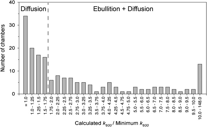
FIGURE 3. The frequency distribution of the ratio of the observed gas transfer coefficient in a given chamber to the minimum gas transfer coefficient observed during a given set of chamber deployments (k₆₀₀/k₆₀₀ Minimum) was used to differentiate between diffusive and ebullitive surface water methane emissions. The threshold of 1.75 was determined by statistical change point detection.

Estimations of CH₄ Oxidation

Microbial oxidation of CH₄ in either oxic shallow sediment layers or surface waters results in an increase in δ¹³C-CH₄ values relative to its origin (Bastviken et al., 2002). Thus, we calculated the extent to which MOX limits diffusive surface water methane emissions by comparing surface water δ¹³C-CH₄ to both bubble and porewater δ¹³C-CH₄. We applied two different models to assess the largest range of uncertainty. We used a model that represents an open system at steady state (Eq. 7) (Happell et al., 1994) and a second Rayleigh model for closed systems (Eq. 8) (Sawakuchi et al., 2016) to calculate the fraction of CH₄ oxidized in shallow sediments and surface waters (f):

$f=\frac{{\text{δ}}_{\text{SW}}- {\text{δ}}_{\text{b}}}{\left(a-1\right) x 1000}(7)$

$\ln \left(1-f\right)=\frac{\ln \left({\text{δ}}_{\text{b}}+1000\right)- \ln \left({\text{δ}}_{\text{SW}}+1000\right)}{a-1}(8)$

where δ_SW is the δ¹³C-CH₄ of surface waters, δ_b is the δ¹³C-CH₄ of bubbles and/or porewater, and a is the isotopic fractionation factor. Each calculation was made using two fractionation factor values—1.025 and 1.033—representative of the range of literature values available for similar systems (Tyler et al., 1997; Zhang et al., 2013). We also made the calculations using δ¹³C-CH₄ from bubbles and both porewater depths considering it was not always logistically possible to collect bubbles in shallow waters. We present MOX estimations as the average ± 1 SE of all calculations (i.e., two equations, two a values, and one or more belowground δ¹³C-CH₄ values).

Spatial Scaling of CH₄ Fluxes

We estimated total annual CH₄ emissions from each wetland in order to evaluate 1) the contribution of each flux pathway to wetland-scale CH₄ emissions and 2) the sustained global warming potential impact of CH₄ emissions compared to OC burial in the wetland sediments. The hydrology and topographic setting of the studied wetlands are extensively described by McLaughlin et al. (2019). In short, we measured water levels continuously for the entire study period using pressure transducers (Solinst Gold Levelogger) deployed in shallow groundwater wells situated in the deepest part of each wetland. Barometric pressure correction was performed using data collected from barometric pressure transducers (Solinst Barologger) deployed in a dry well adjacent to each water level recorder. LIDAR digital elevation models were provided by the National Center for Airborne Laser Mapping, processing of the LIDAR digital elevation models are described in detail in Quintero and Cohen (2019). Elevations are reported with an estimated mean accuracy of 5 cm across each domain, and with a spatial resolution of 5 m. The surface area of the center, intermediate, and edge sections of each wetland were determined based on elevation thresholds that aligned with shifts in vegetation coverage and inundation extent. Edge delineations capture the entirety of the wetland depression within the delineated extent while making sure to exclude any upland area. Intermediate delineations capture the bald/pond cypress extent of each wetland while making sure to exclude dwarf cypress and pine at higher elevations. Center delineations capture the center communities in our domes, these include open water areas, which typically differ from the dominant cypress community.

Surface water CH₄ fluxes were multiplied by the percentage of the year that each section was inundated and soil CH₄ fluxes were multiplied by the percentage of the year that was dry. To scale the knee surface area we used an available literature value for the density of knees (0.315 knees m⁻²) in a similar cypress swamp setting since knee density was not measured in this study (Pulliam, 1992). Pulliam (1992) determined knee density across two 1,250 m transects in the frequently inundated lower floodplain of the Ogeechee River with 1 m² plots established every 8m (i.e., 156 plots per transect).We then multiplied this knee density by the average surface area of knees that we made flux measurements on (0.57 m² knee⁻¹), and finally multiplied by the landscape surface area of each compartment. TR3 had no cypress trees or knees, whereas the other wetlands had knees in qualitatively similar abundance from the center to edge. Due to logistical constraints (i.e., time constraints), knee CH₄ flux measurements were not able to be made in each wetland section, thus, in those cases the average flux rate for a given wetland was applied to each of its sections.

Carbon burial rates were estimated for the center of each wetland based on previously reported 210Pb sediment accumulation rates, which were not measured for the intermediate and edge wetland sections (Zhang et al., 2019). 210Pb dating was performed down to 42 cm at the RP3 wetland and we applied this same rate to the other three wetlands. OC abundance in sediments (%OC) and bulk density were measured every 1 cm (Zhang et al., 2019). We used the average %OC and bulk density down to 42 cm to match the 210Pb time frame for carbon burial estimates. Carbon burial rates were determined as follows:

$\text{OC Burial}=\%\text{OC} x \text{Bulk Density} x S\text{ediment Accumulation Rate} x \text{Surface Area}(9)$

The ratio of methane emissions to OC burial was calculated to compare their relative rates. This ratio was then multiplied by the sustained global warming potential of CH₄ for 20, 100, and 500 yr time frames (Neubauer and Megonigal, 2015) to determine the net balance in atmospheric radiative forcing from CH₄ emissions and CO₂ uptake by vegetation and subsequent burial as OC in sediments.

Data Analysis

All statistical analyses were performed in the statistical computing language R using R Studio version 1.3.1093 (RStudio Team, 2020). Calculations of the k₆₀₀/k_600-min threshold for ebullition to occur described in CH₄fluxes From Surface Water, Soils, and Cypress Knees were performed using the “changepoint” R package. The changes in mean (cpt.mean) function was used with the At Most One Change (AMOC) method and the Modified Bayesian information criterion (MBIC) penalty. The change point of k₆₀₀/k_600-min was determined to be 1.75 with a confidence value of 1.00.

Field data was determined to not have a normal distribution based on visual inspection of density and QQ plots. Thus, we chose the non-parametric unpaired Wilcoxon test to evaluate the statistical significance of differences in measured parameters (e.g., pCH₄, δ¹³C-CH₄, CH₄ fluxes, and MOX) between wetland sites, sampling stations (i.e., center, intermediate, and edge), measurement types (e.g., soil vs. surface water fluxes), and sampling season. For example, we used the Wilcoxon test to determine if a given flux pathway was significantly higher at the site with the highest average flux rate compared to each of the other three sites individually. Thus, reported p values represent comparisons of one group to another (e.g., TR2 vs. RP1, TR2 vs. RP3, etc.). Significant differences were considered to fall within a 95% confidence interval (i.e., p < 0.05). In cases where all comparisons yielded insignificant differences (e.g., no wetland sites were statistically distinct from one another) we report the range of computed p values as (maximum p value < p > minimum p value) for the sake of brevity.

We performed linear regressions to determine correlations between measured parameters (i.e., pCH₄ vs. δ¹³C-CH₄, fluxes vs. temperature, and fluxes vs. wetland stage) and report R² values.

All data is reported as the average ± standard error of the mean. This standard error was propagated through our estimations of total wetland methane emissions. The distribution and variability of field data is shown in box plots (Figures 4–6).

FIGURE 4

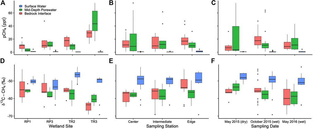
FIGURE 4. The partial pressure of CH₄ measured in surface water and porewater sampled near the bedrock interface and midway between the bedrock and sediment surface sorted by (A) site and (B) season. The stable isotopic composition of CH₄ (δ¹³C-CH₄) is also shown by (C) site and (D) season. Panels A and C include measurements made at the center, intermediate, and edge sampling locations for each wetland. Panels B and D include measurements made at all sampling locations and wetlands.

FIGURE 5

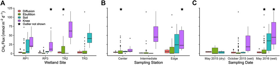
FIGURE 5. Big Cypress methane fluxes from surface water diffusion, surface water ebullition, non-inundated soils, and cypress knees by (A) site, (B) sampling station, and (C) sampling period. Stars indicate one outlier present outside the displayed axis scale.

FIGURE 6

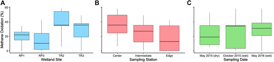
FIGURE 6. The percentage of methane that was microbially oxidized in surface waters prior to outgassing via diffusion by (A) site, (B) sampling station, and (C) sampling period.

Results

CH₄ Concentrations and Stable Isotopic Composition

Methane measurements were made during two dry seasons (May 2015 and 2016) and one wet season (October 2015). Wetland stage was lower immediately before and after the May 2015 sampling, whereas wetland stage was relatively high during the May 2016 dry season compared to 2015 and 2017 (Figure 1D). The partial pressure of CH₄ in surface waters varied from 0.148 to 4.53 ppt with an average of 0.805 ± 0.128 ppt throughout the study period (Figures 4A–C). The δ¹³C-CH₄ of surface waters ranged from -69.2 to -42.0‰ with an average of -50.3 ± 0.8‰ throughout the study period (Figures 4D–F). Surface water pCH₄ was highest on average at RP1 (1.31 ± 0.128 ppt) compared to RP3 (1.00 ± 0.284 ppt; p = 0.60), TR3 (0.654 ± 0.239 ppt; p = 0.06), and TR2 (0.477 ± 0.068 ppt; p = 0.05) (Figure 4A). The most enriched average δ¹³C-CH₄ values (−46.7 ± 0.7‰) were observed TR2, which also had the lowest pCH₄ and this difference in δ¹³C-CH₄ was significant (p = 0.00 when comparing TR2 to each wetland individually) (Figure 4D). Average δ¹³C-CH₄ values were more similar to each other at RP1 (−50.2 ± 0.5‰), RP3 (−53.7 ± 1.8‰), and TR3 (−53.0 ± 2.6‰) with no statistically significant differences (0.79 < p > 0.16 when comparing each wetland to one another). There was also no significant difference between the center, midway point, or edge of the wetlands for surface water pCH₄ (0.79 < p > 0.16) and δ¹³C-CH₄ (0.74 < p > 0.58) (Figures 4B,E). Finally, there were no statistically significant differences in surface water pCH₄ (0.66 < p > 0.28) or δ¹³C-CH₄ (0.45 < p > 0.26) when comparing each sampling season (Figures 4C,F).

Porewater CH₄ concentrations ranged from 0.748 to 75.2 ppt with an average of 16.1 ± 1.85 ppt. The δ¹³C-CH₄ of porewaters ranged from −69.1‰ to −43.3‰ with an average of −57.0 ± 0.6‰ throughout the study period. Average pCH₄ in pore waters was 20 times higher than surface waters (p = 0.00) and porewater δ¹³C-CH₄ was more 6.7‰ more depleted than surface waters (p = 0.00) (Figure 4). Porewater collected at mid-depth had an average pCH₄ that was 1.1 times higher than at the bedrock interface, but this difference was not significant (p = 0.35). Likewise, average porewater δ¹³C-CH₄ at mid-depth (-57.7 ± 0.7‰) was slightly more depleted than at the bedrock interface (-56.5 ± 0.9‰; p = 0.28), but this difference was not significant.

Seasonally, the highest average porewater pCH₄ occurred during the October 2015 high wetland stage period (17.9 ± 2.32 ppt) compared to the low wetland stage May 2015 period (14.4 ± 7.35 ppt; p = 0.03) and moderate wetland stage May 2016 period (13.2 ± 2.63 ppt; p = 0.07) (Figure 4C). δ¹³C-CH₄ was the most depleted in May 2016 (−59.1 ± 1.3‰) compared to May 2015 (−55.7 ± 1.0‰; p = 0.09) and October 2015 (−56.3 ± 0.8‰; p = 0.07) (Figure 4F). Porewater pCH₄ at the bedrock interface was highest at TR3 (28.0 ± 3.75 ppt) compared to TR2 (16.0 ± 2.82 ppt; p = 0.02), RP3 (14.3 ± 3.65 ppt; p = 0.02), and RP1 (16.0 ± 3.65 ppt; p = 0.00) (Figure 4A). Following the same trend, δ¹³C-CH₄ at the bedrock interface was 9.0–10.5‰ more depleted at TR3 compared to the other wetlands (p = 0.00) (Figure 4D). Porewater pCH₄ at mid-depth was even more elevated at TR3 (46.7 ± 7.92 ppt) compared to RP3 (11.1 ± 2.18 ppt; p = 0.00), TR2 (8.30 ± 1.40 ppt; p = 0.00), and RP1 (3.29 ± 0.917 ppt; p = 0.00) (Figure 4A). The difference in δ¹³C-CH₄ between sites was not as large for mid-depth porewaters; TR3 was 2.7–5.2‰ more depleted at TR3 compared to the other wetlands (0.23 < p > 0.00). In general, pCH₄ was not correlated with δ¹³C-CH₄ for either surface or porewaters (R² = 0.12 and 0.03, respectively), except for surface waters at TR3, where pCH₄ was negatively correlated with δ¹³C-CH₄ (R² = 0.89).

The pCH₄ of bubbles collected from the sediment-surface water interface ranged from 55.0 to 1,000 ppt (i.e., pure CH₄) for all sites with an average value of 376 ± 71.1 ppt. The average δ¹³C-CH₄ of bubbles was −61.3 ± 0.68‰, which was 4.3% more depleted than porewaters (p = 0.00). Because bubbles were not always able to be collected (e.g., when surface water level was too low for the sampling funnel), we did not attempt statistical comparisons between wetland sites, seasons, or sampling stations.

CH₄ Flux Rates

The total flux rate of CH₄ from surface waters to the atmosphere (F_T) for all floating chamber deployments ranged from 0.17 to 137 mmol m⁻² d⁻¹ with an average of 11.3 ± 1.45 mmol m⁻² d⁻¹. The highest F_T rates were observed in May 2016 (16.2 ± 3.22 mmol m⁻² d⁻¹) compared to May 2015 (11.4 ± 3.22 mmol m⁻² d⁻¹; p = 0.38) and October 2015 (8.19 ± 1.39 mmol m⁻² d⁻¹; p = 0.14) (Figure 5C). The TR2 wetland had the highest F_T rates (17.3 ± 3.86 mmol m⁻² d⁻¹) compared to RP1 (12.0 ± 2.91 mmol m⁻² d⁻¹; p = 0.77), TR3 (10.7 ± 2.48 mmol m⁻² d⁻¹; p = 0.65), and RP3 (3.95 ± 0.64 mmol m⁻² d⁻¹; p = 0.05) (Figure 5A).

The gas transfer coefficient (k₆₀₀) for surface water fluxes ranged from 0.002 to 18.0 m d⁻¹ (average = 0.711 ± 0.14 m d⁻¹). The k₆₀₀/k_600-min ratio for each deployment of five chambers reached as high as 148 in the case of high ebullition, with an average of 4.82 ± 0.91 (Figure 3). Based on k₆₀₀/k_600-min ratio, we separated out F_T into surface water fluxes derived from diffusion and ebullition (F_D and F_E, respectively) for each deployment. Average CH₄ ebullition rates for all four wetlands combined (7.79 ± 1.37 mmol m⁻² d⁻¹) were 2.2 times higher than diffusion rates (3.50 ± 0.22 mmol m⁻² d⁻¹; p = 0.00); F_T accounted for 69% of the total surface water CH₄ flux rate on average. Similar to F_T, the ebullitive flux F_E was highest in May 2016 (12.5 ± 3.01 mmol m⁻² d⁻¹) compared to May 2015 (6.87 ± 3.15 mmol m⁻² d⁻¹; p = 0.38) and October 2015 (4.92 ± 1.33 mmol m⁻² d⁻¹; p = 0.03) (Figure 5C). In contrast, the diffusive surface water flux F_D was highest during the May 2016 sampling (4.57 ± 0.44 mmol m⁻² d⁻¹) compared to May 2015 (3.72 ± 0.41 mmol m⁻² d⁻¹; p = 0.03) and October 2016 (3.26 ± 0.28 mmol m⁻² d⁻¹; p = 0.03) (Figure 5C).

Across sites, F_D was highest at RP1 (4.72 ± 0.63 mmol m⁻² d⁻¹) compared to TR3 (3.68 ± 0.43 mmol m⁻² d⁻¹; p = 0.14), TR2 (3.21 ± 0.27 mmol m⁻² d⁻¹; p = 0.69), and RP3 (2.31 ± 0.32 mmol m⁻² d⁻¹; p = 0.00) (Figure 5A). In contrast, F_E was highest at TR2 (14.0 ± 3.75 mmol m⁻² d⁻¹) compared to RP1 (12.0 ± 2.91 mmol m⁻² d⁻¹; p = 0.14), TR3 (7.04 ± 2.48 mmol m⁻² d⁻¹; p = 0.34), and RP3 (3.95 ± 0.64 mmol m⁻² d⁻¹; p = 0.08). F_T at the wetland edge stations were 1.6 and 2.6 times higher than the center (p = 0.39) and intermediate stations (p = 0.00), respectively (Figure 5B). Likewise, F_D at the wetland edge stations were 1.5 and 3.9 times higher than the center (p = 0.05) and intermediate stations (p = 0.00), respectively. FE was also 1.6 and 2.3 times higher at the edge stations compared to center (p = 0.32) and intermediate stations (p = 0.73), respectively, but this difference was less statistically significant likely due to higher variability (Figure 5B).

The average flux rate of CH₄ from soils (F_S) that were not inundated during the time of sampling (18.4 ± 5.14 mmol m⁻² d⁻¹) was 1.6 times higher than the total flux from surface waters, but this difference was not statistically significant (p = 0.77). However, there was a more significant difference between F_S and F_D and F_E when considered separately (p = 0.06 and 0.00, respectively). F_S was substantially higher in May 2016 (34.8 ± 8.31 mmol m⁻² d⁻¹) compared to both May 2015 (3.56 ± 1.01 mmol m⁻² d⁻¹; p = 0.02) when water levels were substantially lower and October 2015 when only non-inundated soils were present at RP1 (2.85 ± 1.69 mmol m⁻² d⁻¹; p = 0.29) (Figure 5C). F_S was substantially higher at TR3 (44.8 ± 13.9 mmol m⁻² d⁻¹) compared to RP1 (18.7 ± 7.01 mmol m⁻² d⁻¹; p = 0.10), RP3 (4.41 ± 1.39 mmol m⁻² d⁻¹; p = 0.03), and TR2 (0.718 ± 0.035 mmol m⁻² d⁻¹; p = 0.06) (Figure 5A).

The average flux of CH₄ from cypress knees (F_K; 42.0 ± 6.33 mmol m⁻² d⁻¹) was 3.7 and 2.3 times higher than F_T (p = 0.00) and F_S (p = 0.00), respectively. F_K was 2.1 times higher in May 2016 (58.2 ± 10.8 mmol m⁻² d⁻¹) compared to October 2016 (27.6 ± 5.48 mmol m⁻² d⁻¹; p = 0.01), and was not sampled in May 2015 (Figure 5C). F_K was highest at TR2 (65.1 ± 8.46 mmol m⁻² d⁻¹) compared to RP1 (33.5 ± 7.31 mmol m⁻² d⁻¹; p = 0.01) and RP3 (31.0 ± 11.2 mmol m⁻² d⁻¹; p = 0.00) (Figure 5A). Cypress knees are not present at TR3. The higher cypress knee flux rates at TR2 may be linked to elevated porewater pCH₄ at that site (Figure 4A). The highest average F_K rates were observed at intermediate sampling stations (54.7 ± 7.76 mmol m⁻² d⁻¹) compared to edge stations (45.9 ± 13.1 mmol m⁻² d⁻¹; p = 0.18) and center stations (12.1 ± 4.67 mmol m⁻² d⁻¹; p = 0.00) (Figure 5B), but there was not a significant difference between porewater concentrations by station (0.99 < p > 0.36) (Figure 4B). CH₄ fluxes were not correlated to either temperature or wetland stage for F_T, F_D, F_E, F_S, or F_K (0.17 < R² > 0.00).

Microbial Oxidation of CH₄

On average, we estimate that 26 ± 3% of the CH₄ diffused from soil porewaters into surface waters is oxidized to CO₂ before evasion to atmosphere, resulting in an observed surface water diffusive CH₄ flux (i.e., F_D) that is 26% lower than the rate of CH₄ input to surface waters from sediments. The extent of MOX was higher in the TR wetlands than the RP wetlands (Figure 6A); TR2 had the highest extent of MOX on average (40 ± 5%), which was 1.4 times higher than TR3 (28 ± 7%; p = 0.46), 2.0 times higher than RP1 (20 ± 5%; p = 0.01), and 2.7 times higher than RP3 (15 ± 7%; p = 0.04). There was no significant variability between sampling period for the wetlands when all wetlands were considered together (1.00 < p > 0.37) (Figure 6C). MOX was highest in the center sampling stations (35 ± 6%) compared to intermediate stations (25 ± 5%; p = 0.17) and edge stations (18 ± 7%; p = 0.11) (Figure 6B), but these differences were not significant.

Spatially-Scaled CH₄ Fluxes and Carbon Burial

The low elevation center of each dome comprised 3–12% of the surface area of the studied wetlands. The intermediate and edge (i.e., mid to high elevation) sections comprised of 25–47% and 49–88% of each wetland, respectively (Table 2). The center, intermediate, and edge components were non-inundated (i.e., no surface water) 9–17%, 15–27%, and 16–46% of the study period, respectively. The total flux of CH₄ from each wetland ranged from 239 ± 70 kg C yr⁻¹ for the small RP3 wetland to 1741 ± 220 kg C yr⁻¹ for the larger RP1 wetland. Diffusion and ebullition of methane from surface waters to the atmosphere contributed to 14 ± 2% (range = 8–17%) and 25 ± 6% (range = 12–34%) of the total spatially-scaled flux estimates from all four wetlands, respectively (Table 2). Methane emissions from non-inundated soils contributed to 34 ± 10% of the total spatially-scaled flux estimates from all four wetlands, but had a much larger range (1–71%) for each individual wetland compared to surface water fluxes (Table 2). Cypress knees contributed to 26 ± 5% of the total spatially-scaled flux estimates from all four wetlands. Knees were not present at TR3. When only considering the other three wetlands, knees accounted for 39 ± 5% of the total scaled methane fluxes with a range of 24–75% for each individual wetland. These totals do not include fluxes from the stems and leaves of the cypress trees, which is likely to increase the total.

TABLE 2

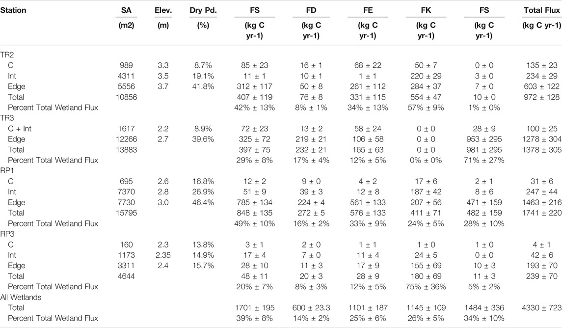
TABLE 2. Summary of surface area (SA), elevation delineations (Elev), the percentage of the year without inundation (Dry Pd), and spatially scaled total surface water methane fluxes (F_T), diffusive surface water fluxes (F_D), ebullitive surface water fluxes (F_E), methane fluxes from cypress knees (F_K), and methane fluxes from soils (F_S).

OC burial rates over the last century were estimated for the dome centers based on a sediment accretion rate of 0.45 cm yr⁻¹ (Zhang et al., 2019). %OC averaged across the top 42 cm ranged from 13.5% to 19.1% for each wetland center and bulk density ranged from 1.20 to 1.37 g cm⁻³ (Table 3). Carbon burial rates ranged from 160 kg C yr⁻¹ for the small RP3 wetland to 1,263 kg C yr⁻¹ for TR3. The molar ratio of CH₄ emissions to OC burial ranged from 0.03 to 0.14, or, in other words, spatially-scaled OC burial rates were 7–36 times greater than total spatially-scaled CH₄ emissions from the wetland centers. When ecosystem CH₄ emissions are sustained (as opposed to a one-time pulse), CH₄ has a sustained global warming potential of 96, 45, and 11 times that of CO₂ on 20 yr, 100 yr, and 500 yr timescales (Neubauer and Megonigal, 2015). Over the 20 and 100 yr time frames, the wetland centers of all four wetland sites were a net source of warming potential to the atmosphere; i.e., the methane they emitted to the atmosphere had a larger greenhouse gas impact than the CO₂ removed from the atmosphere by vegetation that gets buried in sediments as OC (Table 3). The ratio of methane warming potential to carbon burial ranged from 2.7–13.3 and 1.3–6.3 for 20 yr and 100 yr time frames, respectively (Table 3). Over the 500 yr time frame the wetland centers at three wetland sites were net sinks of warming potential (i.e., OC burial outweighed the impact of CH₄ emissions) with the ratio of methane warming potential to carbon burial ranging from 0.3–0.9. TR2 was a net source of warming potential even over 500 yr time scales with a warming potential ration of 1.5 (Table 3).

TABLE 3

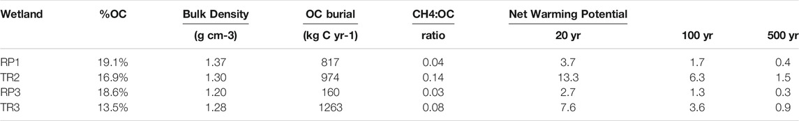
TABLE 3. The percent organic carbon (%OC) and bulk density of sediments, OC burial rates, the molar ratio of total methane fluxes to OC burial, and net warming potential of the wetland centers from 20–500 yr timescales. Net warming potential values above 1 indicate the wetland is a net source of atmospheric warming and values below 1 indicate that the wetland is a net sink (i.e., has a net cooling effect).

Discussion

Pathways for Methane Emissions and Oxidation

Our results show that the total flux of CH₄ from cypress dome surface waters was not significantly different from non-inundated soil CH₄ fluxes on the wetland edge or during periods of low water levels (Figure 5). Likewise, our observed methane flux rates from soils and surface waters (diffusion + ebullition) were nearly equivalent to other chamber-based measurements made in similar subtropical wetlands in Florida such as Corkscrew Swamp, FL (11.2 mmol m² d⁻¹ compared to 11.3 mmol m² d⁻¹ in this study) (Villa and Mitsch, 2014; Pereyra and Mitsch, 2018). The deep slough of the Corkscrew Swamp riverine cypress strand, which accumulates peat, is most similar to the cypress domes we studied, whereas the other four topographic settings studied by Villa and Mitsch (2014) were more similar to the unstudied upland settings surrounding our study domain and had an order of magnitude lower flux rates. Our average flux rates for surface water diffusion were also comparable to average rates reported for subtropical wetlands in a synthesis of global wetland studies, whereas our observed flux rates for total surface water emissions (diffusion + ebullition) was 2.8 times higher, soil emissions were 4.6 times higher, and knee emissions were 10.5 times higher (Turetsky et al., 2014). Only two subtropical wetlands were included in this synthesis, highlighting the paucity of comprehensive GHG data needed to constrain global wetland CH₄ budgets, which represent nearly half of all natural sources of CH₄ to the atmosphere (Saunois et al., 2020).

Cypress knees were the most rapid pathway for methane release in our study with flux rates 3.7 and 2.3 times higher than total surface water and soil flux rates, respectively (Figure 5). The highest knee flux rates were observed at the wetland site with the highest porewater pCH₄ (TR2) suggesting that subsurface methane content is an important driver of emissions through emergent root structures and perhaps also tree stems (Barba et al., 2019a), which were not studied here. Cypress knees represent a relatively small feature of the landscape in a two-dimensional plane, however, unlike the soil and water surface, gas exchange occurs from its entire three-dimensional structure. This attribute, along with the high measured flux rates, scales to represent a substantial percentage (39 ± 5%) of wetland CH₄ emissions at the three studied wetland sites with cypress trees present. This potentially important emission pathway has only been addressed by several previous studies. Observations made in the floodplain of a southeastern, USA blackwater river concluded that cypress knees contributed to less than 1% of the total methane emissions from the floodplain (Pulliam, 1992). The small contribution of cypress knees compared to floodplain surface CH₄ emissions in this case was likely due to substantially lower porewater CH₄ concentrations that resulted in average knee CH₄ flux rates that were ∼45 times lower than our measured rates. Knee CH₄ flux rates measured in the Sabine River floodplain in S.E. Texas were similar in magnitude to our measurements and it was reported that vegetation contributed to 64–96% of total ecosystem methane release (Bianchi et al., 1996). In that case the measured porewater CH₄ concentrations at depths greater than ∼10 cm were the same order of magnitude as our observations, whereas surface soils had nearly undetectable CH₄ levels, and surface waters had measurable rates of CH₄ oxidation.

Understanding the mechanisms that drive methane cycling through each pathway is a prerequisite for determining how effectively wetlands act as sources or sinks of GHGs and how they feedback and interact with changes to the Earth system. Water level is considered to be the primary factor that controls soil methane emissions in wetlands, particularly in tropical and subtropical wetlands that have wet and dry seasons (Whalen, 2005; Mitsch et al., 2010). Mitsch et al. (2010) observed that tropical wetlands with seasonal pulses in water level (e.g., monsoon cycles) had higher total annual methane emissions than permanently flooded wetlands, and that the highest seasonal emissions occurred when water levels were between 15–30 cm above the ground surface. This relationship to depth has also been observed in ombrotrophic peatlands and in both cases was attributed to enhanced MOX in shallow soils when water levels are low enough to allow soil aeration and enhanced MOX in surface waters when surface water depths are greater (Jauhiainen et al., 2005), which aligns with our observations of higher MOX in the wetland centers compared to edge (Figure 6B).

The open water environments in BICY are small and shallow, which favor CH₄ ebullition due to low hydrostatic pressure and plant mediated fluxes from the predominantly anoxic porewater environments. MOX decreased the diffusive flux from open water by 26 ± 3% in the BICY wetlands (Figure 6). However, the extent of MOX observed in our study area was considerably lower than reported in a large tropical floodplain lake in the Amazon (Barbosa et al., 2018), which found that in some cases up to 100% of the methane delivered from sediments to surface waters was oxidized. Future studies are needed to resolve the drivers of the large variability in MOX across different wetlands, and thereby better predict the conditions under which MOX significantly limits wetland methane emissions. Studies in rivers and lakes have identified some factors that influence the extent of MOX. For example, a lab incubation study showed that methane formation rates in lake sediments increased with increasing temperatures, whereas MOX potential was more closely related to CH₄ concentrations rather than temperature or sediment type (Duc et al., 2010). In rivers, NH₄⁺ concentrations above 20 μmol L⁻¹ and light exposure have both been shown to inhibit MOX (de Angelis and Scranton, 1993; Dumestre et al., 1999), whereas MOX generally increases with higher suspended sediment concentrations (Weaver and Dugan, 1972). The high light exposure to the shallow waters at BICY, low suspended sediment concentrations (mean = 5–7 mg L⁻¹; 1974–1994), and historic mean NH₄⁺ concentrations of 13–20 μmol L⁻¹ (Lietz, 2000) are all factors that may result in low MOX compared to other wetland systems.

Methane emissions from woody vegetation, which has only recently received significant attention (Barba et al., 2019a), are linked to several mechanisms relevant to our measurements. One mechanism for methane emissions from woody plants appears to be similar to herbaceous plants, whereby they take up soil-derived CH₄ by the root system (Covey and Megonigal, 2019). Stem methane emissions are not related to transpiration (Barba et al., 2019b), suggesting that diffusion through the plant’s cells is the physical mechanism for methane exchange. For example, though plant adaptations such as aerenchyma and lenticels for increased O₂ diffusion in anoxic or water-logged environments can facilitate root-mediated transport of soil-produced methane (Pangala et al., 2013), transport of soil-derived CH₄ through tree stems has also been found in plants without these structures (Maier et al., 2018). Thus, regardless of whether or not cypress knees actively provide O₂ to roots in anoxic soil layers, diffusion of methane from soils to the atmosphere through knees is likely to occur, resulting in the high flux rates we observed. Methane can also be produced inside the biomass of woody vegetation by methanogenic archaea (Zeikus and Ward, 1974; Yip et al., 2019). This phenomenon is typically attributed to trees in upland forests with high CH₄ flux rates even when soils exhibit net uptake of methane (Barba et al., 2019b), though it is certainly possible that trees in wetland environments both transport methane from soils and produce it internally depending on the redox state and microbiome of woody biomass.

Woody vegetation plays an important role in CH₄ emissions in the case of environments with elevated porewater concentrations and high amounts of oxidation in shallow soils and/or surface waters. For example, average porewater pCH₄ was 20 times greater than surface water pCH₄ in our study (Figure 4). The roots of trees, which sample water and solutes from deeper soils than herbaceous plants, act as a direct conduit for methane to vent from deep soil porewaters with limited exposure to settings where oxidation occurs. On the other hand, O₂ may enter sediments from tree roots, oxidizing the rhizosphere and enabling MOX to occur deeper in the sediment than one might expect. This may explain several of the relatively high porewater δ¹³C-CH₄ values observed (i.e., maximum of −43.3‰), while the average porewater δ¹³C-CH₄ values (−57.0 ± 0.6‰) fall in the range of acetoclastic rather than hydrogenotrophic methanogenesis. Tree stems may contribute even more than knees to whole ecosystem methane fluxes because of their greater surface area and height, though few studies have shown how CH₄ fluxes change along the radial and vertical axes of a stem (Jeffrey et al., 2020). Tree-mediated methane emissions contribute 9–27% and 44–65% of the total ecosystem CH₄ flux in forested temperate and tropical wetlands, respectively (Pangala et al., 2017). Similar to methane emissions, the soil depths where methane oxidation can occur are linked to water level (Whalen and Reeburgh, 2000). Thus, the extent of wetland tree CH₄ emissions are likely linked to the interplay between rooting depth, water table depth, and redox zonation along the soil profile.

Comparison of Wetland Methane Emissions and Organic Carbon Burial

Are freshwater wetlands net sources or sinks of atmospheric GHGs and over what timescales? This critical question has been addressed in previous studies using the molar ratio between wetland CH₄ emissions and CO₂ uptake. These values ranged from 0.05–0.06 for two subtropical wetlands, 0.09–0.11 for two temperate wetlands, and 0.13–0.20 for three high-latitude wetlands (Whiting and Chanton, 2001). Our estimates were in the same range as subtropical wetlands studied by Whiting and Chanton (2001) (0.04–0.08) with the exception of TR2 (0.14) (Table 3), which had the highest knee flux rates and highest rates of ebullition from sediments (Figure 5A). Whiting and Chanton (2001) used global warming potential values of CH₄ based on the lifetime of a single pulse of CH₄ in the atmosphere (20 yr = 21.8, 100 yr = 7.6, 500 yr = 2.5) (Lelieveld et al., 1993) to reach the conclusion that all of their studied wetlands were net sinks of warming potential over a 500 yr time frame and the subtropical wetlands were also net sinks over a 100 yr time frame. We used updated global warming potentials based on a sustained flux of methane from an ecosystem, which are considerably higher (20 yr = 96, 100 yr = 45, 500 yr = 11; (Neubauer and Megonigal, 2015) to reach the conclusion that, over 100 yr timescales, the subtropical wetlands we studied are net sources of warming potential in contrast to prior studies.

There is not a clear consensus on what timescales are most important to consider with respect to global warming potential (Myhre et al., 2013; Kirschbaum, 2014). The 100 yr time frame represents the lifetime of CO₂ in the atmosphere—an order of magnitude longer than the residence time of CH₄—and the time it generally takes terrestrial ecosystems to reach successional steady state (Odum, 2014). The 500 years time frame is similar to the time period over which ocean circulation exerts an important influence on climate change (Lelieveld et al., 1998). For context, the BICY patterned landscape appears to have begun forming in the middle to late Holocene (Chamberlin et al., 2018) and the dominant vegetation shifted from herbaceous to woody vegetation ∼3,000 years before present as precipitation and hydroperiods increased (Zhang et al., 2019). Radiocarbon dating of long-chain fatty acids showed that sediment accretion rates in the BICY wetlands were an order of magnitude slower from 1,600 to 3,500 years before present (0.03 cm yr⁻¹ vs. 0.45 cm yr⁻¹ present-day) (Zhang et al., 2019). Although we have no way of measuring past methane emissions, it is possible that carbon burial and methane emission rates have maintained a similar relative balance throughout the various stages of the wetland system’s development, i.e., as carbon burial increases, so do CH₄ emissions. On the other hand, if woody vegetation is in fact a dominant pathway for deep soil methane to bypass oxidation, the wetlands may have shifted from a net sink to net source of greenhouse potential after the vegetation shift towards woody species around 3,000 years ago.

Results from this study build upon a growing body of work demonstrating the importance of wetlands for methane emissions and thus their contributions to climate change (Zhang et al., 2017). Model simulations suggest that natural wetland methane emissions may be a positive feedback for warming. This feedback may be amplifying anthropogenic radiative forcing by up to 5% by 2100, similar to increases in anthropogenic methane emissions over the same time scales (Gedney, 2004). Our results further demonstrate that emergent vegetation is an important flow path for releasing methane from wetland soils as it limits the amount of methane oxidized in surface waters and shallow soils. While the role of herbaceous plants on wetland methane emissions is represented in current global scale Earth system models, the role of woody vegetation is crudely parameterized (Riley et al., 2011). Adding mechanistic detail to predictive models is paramount for fully constraining the role of wetlands as a positive feedback for warming and, likewise, predicting the impact of natural and anthropogenic changes to hydrological regimes on wetland carbon cycling.

Data Availability Statement

The datasets presented in this study can be found in online repositories. The names of the repository/repositories and accession numbers can be found below: https://doi.org/10.6084/m9.figshare.c.4791546.

Author Contributions

TB, JM, and MC led the Big Cypress project and oversaw field and lab activities. CQ organized field logistics and NW performed methane measurements and sample collections. NW and HS performed calculations and data analyses. All authors discussed the results and commented on the manuscript.

Funding

This research was funded by National Science Foundation (DEB#1354783). The Jon and Beverly Thompson Endowed Chair of Geological Sciences to TB also provided support.

Conflict of Interest

The authors declare that the research was conducted in the absence of any commercial or financial relationships that could be construed as a potential conflict of interest.

Acknowledgments

Site access for sample collection was enabled by the U. S. National Park Service under permit BICY‐2016‐SCI‐0008. We gratefully acknowledge assistance and insight from the larger project team including Amy Brown, Catherine Chamberlain, Xiaoli Dong, Madison Flint, Daniel McLaughlin, Brad Murray, Andrea Pain, Adam Watts, Xiaowen Zhang, and James Heffernan. Figure 2 was developed by artist Nathan Johnson. All data can be found in the figures and tables of the manuscript and is also deposited in the figshare repository at: https://doi.org/10.6084/m9.figshare.c.4791546.

References

Anderson, P. H., and Pezeshki, S. R. (2000). The effects of intermittent flooding on seedlings of three forest species. Photosynthetica 37 (4), 543–552.

CrossRef Full Text | Google Scholar

Baker-Blocker, A., Donahue, T. M., and Mancy, K. H. (1977). Methane flux from wetlands areas. Tell’Us 29, 245–250.

CrossRef Full Text | Google Scholar

Barba, J., Bradford, M. A., Brewer, P. E., Bruhn, D., Covey, K., van Haren, J., et al. . (2019a). Methane emissions from tree stems: a new frontier in the global carbon cycle. New Phytol. 22, 18–28. doi:10.1111/nph.15582

CrossRef Full Text | Google Scholar

Barba, J., Poyatos, R., and Vargas, R. (2019b). Automated measurements of greenhouse gases fluxes from tree stems and soils: magnitudes, patterns and drivers. Sci. Rep. 9, 4005. doi:10.1038/s41598-019-39663-8

PubMed Abstract | CrossRef Full Text | Google Scholar

Barbosa, P. M., Farjalla, V. F., Melack, J. M., Amaral, J. H. F., da Silva, J. S., and Forsberg, B. R. (2018). High rates of methane oxidation in an Amazon floodplain lake. Biogeochemistry 137, 351–365. doi:10.1007/s10533-018-0425-2

CrossRef Full Text | Google Scholar

Bastviken, D., Ejlertsson, J., and Tranvik, L. (2002). Measurement of methane oxidation in lakes: a comparison of methods. Environ. Sci. Technol. 36, 3354–3361. doi:10.1021/es010311p

PubMed Abstract | CrossRef Full Text | Google Scholar

Bastviken, D., Santoro, A. L., Marotta, H., Pinho, L. Q., Calheiros, D. F., Crill, P., et al. . (2010). Methane emissions from Pantanal, South America, during the low water season: toward more comprehensive sampling. Environ. Sci. Technol. 44, 5450–5455. doi:10.1021/es1005048

PubMed Abstract | CrossRef Full Text | Google Scholar

Bastviken, D., Cole, J., Pace, M., and Tranvik, L. (2004). Methane emissions from lakes: dependence of lake characteristics, two regional assessments, and a global estimate. Global Biogeochem. Cycles 18, Gb4009. doi:10.1029/2004GB002238

CrossRef Full Text | Google Scholar

Battin, T. J., Luyssaert, S., Kaplan, L. A., Aufdenkampe, A. K., Richter, A., and Tranvik, L. J. (2009). The boundless carbon cycle. Nat. Geosci. 2, 598–600. doi:10.1038/ngeo618

CrossRef Full Text | Google Scholar

Bianchi, T. S., Freer, M. E., and Wetzel, R. G. (1996). Temporal and spatial variability, and the role of dissolved organic carbon (DOC) in methane fluxes from the Sabine River Floodplain (Southeast Texas, USA). Arch. Hydrobiol. 136, 261–287.

Google Scholar

Briand, C. H. (2000). Cypress knees: an enduring engima. Arnoldia 60 (4), 19–25.

PubMed Abstract | CrossRef Full Text | Google Scholar

Bridgman, S. D., Cadillo-Quiroz, H., Keller, J. K., and Zhuang, Q. (2013). Methane emmisions from wetlands: biogeochemical, microbial, and modelling prespectives from local to global scales. Glob. Chang. Biol. 19, 1325–1346. doi:10.1111/gcb.12131

CrossRef Full Text | Google Scholar

Chamberlin, C. A., Bianchi, T. S., Brown, A. L., Cohen, M. J., Dong, X., Flint, M. K., et al. . (2018). Mass balance implies Holocene development of a low-relief karst patterned landscape. Chem. Geol. 527, 118782. doi:10.1016/j.chemgeo.2018.05.029

CrossRef Full Text | Google Scholar

Cohen, M. J., Watts, D. L., Heffernan, J. B., and Osborne, T. Z. (2011). Reciprocal biotic control on hydrology, nutrient gradients, and landform in the greater everglades. Crit. Rev. Env. Sci. Tech. 41 (S1), 395–429.

CrossRef Full Text | Google Scholar

Covey, K. R., and Megonigal, J. P. (2019). Methane production and emissions in trees and forests. New Phytol. 222, 35–51. doi:10.1111/nph.15624

PubMed Abstract | CrossRef Full Text | Google Scholar

de Angelis, M. A., and Scranton, M. I. (1993). Fate of methane in the hudson river and estuary. Global Biogeochem. Cycles 7 (3), 509–523. doi:10.1029/93GB01636

CrossRef Full Text | Google Scholar

DelSontro, T., Beaulieu, J. J., and Downing, J. A. (2018). Greenhouse gas emissions from lakes and impoundments: upscaling in the face of global change. Limnology and Oceanography Letters 3, 64–75. doi:10.1002/lol2.10073

CrossRef Full Text | Google Scholar

Dong, X., Cohen, M. J., Martin, J. B., McLaughlin, D. L., Murray, A. B., Ward, N. D., et al. . (2019). Ecohydrologic processes and soil thickness feedbacks control limestone-weathering rates in a karst landscape. Chem. Geol. 527, 118774.

PubMed Abstract | CrossRef Full Text | Google Scholar

Duc, N. T., Crill, P., and Bastviken, D. (2010). Implications of temperature and sediment characteristics on methane formation and oxidation in lake sediments. Biogeochemistry 100 (1-3), 185–196. doi:10.1007/s10533-010-9415-8

CrossRef Full Text | Google Scholar

Dumestre, J. F., Guézennec, J., Galy-Lacaux, C., Delmas, R., Richard, S., and Labroue, L. (1999). Influence of light intensity on methanotrophic bacterial activity in Petit Saut Reservoir, French Guiana. Appl. Env. Microbiol. 65 (2), 534–539.

Frenzel, P. (2000). “Plant-associated methane oxidation in rice fields and wetlands,” in advances in microbial ecology, editor B. Schink (Boston, MA: Springer US), 85–114.

CrossRef Full Text | Google Scholar

Frenzel, P., and Rudolph, J. (1998). Methane emission from a wetland plant: the role of CH4 oxidation in eriophorum. Plant Soil 202, 27–32.

CrossRef Full Text | Google Scholar

Gedney, N. (2004). Climate feedback from wetland methane emissions. Geophys. Res. Lett. 31, 307. doi:10.1029/2004GL020919

CrossRef Full Text | Google Scholar

Happell, J. D., Chanton, J. P., and Showers, W. S. (1994). The influence of methane oxidation on the stable isotopic composition of methane emitted from Florida swamp forests. Geochim. Cosmochim. Acta. 58, 4377–4388. doi:10.1016/0016-7037(94)90341-7

CrossRef Full Text | Google Scholar

Holgerson, M. A., and Raymond, P. A. (2016). Large contribution to inland water CO2 and CH4 emissions from very small ponds. Nat. Geosci. 9, 222. doi:10.1038/ngeo2654

CrossRef Full Text | Google Scholar

Houweling, S., Dentener, F., Lelieveld, J., Walter, B., and Dlugokencky, E. (2000). The modeling of tropospheric methane: how well can point measurements be reproduced by a global model? J. Geophys. Res. 105, 8981–9002. doi:10.1029/1999JD901149

CrossRef Full Text | Google Scholar

Jauhiainen, J., Takahashi, H., Heikkinen, J. E. P., Martikainen, P. J., and Vasander, H. (2005). Carbon fluxes from a tropical peat swamp forest floor. Glob. Chang. Biol. 11, 1788–1797. doi:10.1111/j.1365-2486.2005.001031.x

CrossRef Full Text | Google Scholar

Jeffrey, L. C., Maher, D. T., Tait, D. R., and Johnston, S. G. (2020). A small nimble in situ fine-scale flux method for measuring tree stem greenhouse gas emissions and processes (SNIFF). Ecosystems 23, 1–14. doi:10.1007/s10021-020-00496-6

CrossRef Full Text | Google Scholar

Katherine, C. (1988). Effect of swamp size on growth rates of cypress (Taxodium distichum) trees. Am. Midl. Nat. 120, 362. doi:10.2307/2426008

CrossRef Full Text | Google Scholar

Kirschbaum, M. U. F. (2014). Climate-change impact potentials as an alternative to global warming potentials. Environ. Res. Lett. 9, 034014. doi:10.1201/b20720-3

CrossRef Full Text | Google Scholar

Lelieveld, J., Crutzen, P. J., and Brühl, C. (1993). Climate effects of atmospheric methane. Chemosphere 26, 739–768. doi:10.1016/0045-6535(93)90458-H

CrossRef Full Text | Google Scholar

Lelieveld, J., Crutzen, P. J., and Dentener, F. J. (1998). Changing concentration, lifetime and climate forcing of atmospheric methane. Tellus B Chem. Phys. Meteorol. 50, 128–150. doi:10.3402/tellusb.v50i2.16030

CrossRef Full Text | Google Scholar

Lietz, A. C. (2000). Analysis of water-quality trends at two discharge stations-one within Big Cypress National Preserve and one near Biscayne Bay-southern Florida, 1966-94. US Department of the Interior, US Geological Survey.

CrossRef Full Text | Google Scholar

Maier, M., Machacova, K., Lang, F., Svobodova, K., and Urban, O. (2018). Combining soil and tree-stem flux measurements and soil gas profiles to understand CH4 pathways in Fagus sylvatica forests. J. Plant Nutr. Soil Sci. 181, 31–35. doi:10.1002/jpln.201600405

Google Scholar

Matthews, E., and Fung, I. (1987). Methane emission from natural wetlands: global distribution, area, and environmental characteristics of sources. Global Biogeochem. Cycles 1, 61–86. doi:10.1029/GB001i001p00061

CrossRef Full Text | Google Scholar

McLaughlin, D. L., Diamond, J. S., Quintero, C., Heffernan, J., and Cohen, M. J. (2019). Wetland connectivity thresholds and flow dynamics from stage measurements. Water Resour. Res. 55, 6018–6032. doi:10.1029/2018WR024652

CrossRef Full Text | Google Scholar

McPherson, B. F. (1974). “The big cypress swamp,” in Environments of south Florida: present and past. Editor P. J. Gleason (Miami, FL: Miami Geological Society), Vol. 2, 8.

CrossRef Full Text | Google Scholar

Mitsch, W. J., and Gosselink, J. G. (2007). Wetlands, 4th Edn. New Jersey: John Wiley & Sons.

Google Scholar

Mitsch, W. J., Nahlik, A., Wolski, P., Bernal, B., Zhang, L., and Ramberg, L. (2010). Tropical wetlands: seasonal hydrologic pulsing, carbon sequestration, and methane emissions. Wetl. Ecol. Manag. 18, 573–586. doi:10.1007/s11273-009-9164-4

Google Scholar

Myhre, G., Shindell, D., Bréon, F. M., Collins, W., Fuglestvedt, J., Huang, J., et al. . (2013). “Anthropogenic and natural radiative forcing,” in Climate change 2013: the Physical Science Basis Contribution of working group to the fifth assessment report of the intergovernmental panel on climate change. Editors. T. F. Stocker, D. Qin, G. K. Plattner, M. Tignor, S. K. Allen, and J. Boschung Cambridge, England: Cambridge University Press, 659–740.

CrossRef Full Text | Google Scholar

Neef, L., van Weele, M., and van Velthoven, P. (2010). Optimal estimation of the present-day global methane budget. Global biogeochem. Cycles 24, GB4024. doi:10.1029/2009GB003661

Google Scholar

Neubauer, S. C., and Megonigal, J. P. (2015). Moving beyond global warming potentials to quantify the climatic role of ecosystems. Ecosystems 18, 1000–1013. doi:10.1007/s10021-015-9879-4

CrossRef Full Text | Google Scholar

Nisbet, R. E., Fisher, R., Nimmo, R. H., Bendall, D. S., Crill, P. M., Gallego-Sala, A. V., et al. . (2009). Emission of methane from plants. Proc. Biol. Sci. 276, 1347–1354. doi:10.1098/rspb.2008.1731

CrossRef Full Text | Google Scholar

Nouchi, I., Mariko, S., and Aoki, K. (1990). Mechanism of methane transport from the rhizosphere to the atmosphere through rice plants. Plant Physiol. 94, 59–66. doi:10.1104/pp.94.1.59

PubMed Abstract | CrossRef Full Text | Google Scholar

Odum, E. P. (2014). “The strategy of Ecosystem development,” in The ecological design and planning reader, Editor. F. O. Ndubisi (Washington, DC: Island Press/Center for Resource Economics), 203–216.

PubMed Abstract | CrossRef Full Text | Google Scholar

Pangala, S. R., Enrich-Prast, A., Basso, L. S., Peixoto, R. B., Bastviken, D., Hornibrook, E. R. C., et al. . (2017). Large emissions from floodplain trees close the Amazon methane budget. Nature 552, 230–234. doi:10.1038/nature24639

CrossRef Full Text | Google Scholar

Pangala, S. R., Moore, S., Hornibrook, E. R., and Gauci, V. 2013). Trees are major conduits for methane egress from tropical forested wetlands. New Phytol. 197, 524–531. doi:10.1111/nph.12031

PubMed Abstract | CrossRef Full Text | Google Scholar

Peacock, M., Audet, J., Jordan, S., Smeds, J., and Wallin, M. B. (2019). Greenhouse gas emissions from urban ponds are driven by nutrient status and hydrology. Ecosphere 10, e02643. doi:10.1002/ecs2.2643

PubMed Abstract | CrossRef Full Text | Google Scholar

Pereyra, A. S., and Mitsch, W. J. (2018). Methane emissions from freshwater cypress (Taxodium distichum) swamp soils with natural and impacted hydroperiods in Southwest Florida. Ecol. Eng. 114, 46–56. doi:10.1016/j.ecoleng.2017.04.019

CrossRef Full Text | Google Scholar

Pezeshki, S. R., Pardue, J. H., and DeLaune, R. D. (1996). Leaf gas exchange and growth of flood-tolerant and flood-sensitive tree species under low soil redox conditions. Tree Physiol. 16, 453–458. doi:10.1093/treephys/16.4.453

CrossRef Full Text | Google Scholar

Pulliam, W. M. (1992). Methane emissions from cypress knees in a southeastern floodplain swamp. Oecologia 91, 126–128. doi:10.1007/BF00317250

PubMed Abstract | CrossRef Full Text | Google Scholar

Purvaja, R., Ramesh, R., and Frenzel, P. (2004). Plant-mediated methane emission from an Indian mangrove. Glob. Chang. Biol. 10, 1825–1834. doi:10.1111/j.1365-2486.2004.00834.x

PubMed Abstract | CrossRef Full Text | Google Scholar

Quintero, C. J., and Cohen, M. J. (2019). Scale‐dependent patterning of wetland depressions in a low‐relief karst landscape. J. Geophys. Res. Earth Surf. 124, 2101–2117. doi:10.1029/2019JF005067

CrossRef Full Text | Google Scholar

Raymond, P. A., Hartmann, J., Lauerwald, R., Sobek, S., McDonald, C., Hoover, M., et al. . (2013). Global carbon dioxide emissions from inland waters. Nature 503, 355–359. doi:10.1038/nature12760

CrossRef Full Text | Google Scholar

Riley, W. J., Subin, Z. M., Lawrence, D. M., Swenson, S. C., Torn, M. S., Meng, L., et al. . (2011). Barriers to predicting changes in global terrestrial methane fluxes: analyses using CLM4Me, a methane biogeochemistry model integrated in CESM. Biogeosciences 8, 1925–1953. doi:10.5194/bg-8-1925-2011

PubMed Abstract | CrossRef Full Text | Google Scholar

RStudio Team (2020). RStudio. Boston, MA: Integrated Development Environment for R. RStudio, PBC.

CrossRef Full Text | Google Scholar

Saunois, M., Stavert, A. R., Poulter, B., Bousquet, P., Canadell, J. G., Jackson, R. B., et al. , (2020). The global methane budget 2000–2017. Earth Syst. Sci. Data, 12 (3), 1561–1623. doi:10.5194/essd-12-1561-2020

Google Scholar

Sawakuchi, H. O., Bastviken, D., Sawakuchi, A. O., Krusche, A. V., Ballester, M. V., and Richey, J. E. (2014). Methane emissions from Amazonian Rivers and their contribution to the global methane budget. Global Change Biol. 20 (9), 2829–2840.

Sawakuchi, H. O., Bastviken, D., Sawakuchi, A. O., Ward, N. D., Borges, C. D., Tsai, S. M., et al. . (2016). Oxidative mitigation of aquatic methane emissions in large Amazonian rivers. Glob. Chang. Biol. 22, 1075–1085. doi:10.1111/gcb.13169

CrossRef Full Text | Google Scholar

Sawakuchi, H. O., Neu, V., Ward, N. D., Barros, M. de. L. C., Valerio, A. M., Gagne-Maynard, W., et al. . (2017). Carbon dioxide emissions along the lower Amazon river. Front. Mar. Sci. 4, 76. doi:10.3389/fmars.2017.00076

CrossRef Full Text | Google Scholar

Schutz, H. (1991). “Role of plants in regulating the methane flux to the atmosphere,” in Trace Gas Emission by Plants, San Diego: Academic Press, 29–63.

PubMed Abstract | CrossRef Full Text | Google Scholar

Segers, R. (1998). Methane production and methane consumption: a review of processes underlying wetland methane fluxes. Biogeochemistry 41, 23–51.

CrossRef Full Text | Google Scholar

Shoemaker, W. B., Barclay Shoemaker, W., Lopez, C. D., and Duever, M. J. (2011). Evapotranspiration over spatially extensive plant communities in the Big Cypress National Preserve, southern Florida, 2007-2010. Scientific Investigations Report. doi:10.3133/sir20115212

CrossRef Full Text | Google Scholar

Turetsky, M. R., Kotowska, A., Bubier, J., Dise, N. B., Crill, P., Hornibrook, E. R., et al. . (2014). A synthesis of methane emissions from 71 northern, temperate, and subtropical wetlands. Glob. Chang. Biol. 20, 2183–2197. doi:10.1111/gcb.12580

Google Scholar

Tyler, S. C., Bilek, R. S., Sass, R. L., and Fisher, F. M. (1997). Methane oxidation and pathways of production in a Texas paddy field deduced from measurements of flux, δl3C, and δD of CH4. Global Biogeochem. Cycles 11, 323–348.

CrossRef Full Text | Google Scholar

Vann, C. D., and Patrick Megonigal, J. (2003). Elevated CO2 and water depth regulation of methane emissions: comparison of woody and non-woody wetland plant species. Biogeochemistry 63, 117–134. doi:10.1023/A:1023397032331

PubMed Abstract | CrossRef Full Text | Google Scholar

Villa, J. A., and Mitsch, W. J. (2014). Methane emissions from five wetland plant communities with different hydroperiods in the big cypress swamp region of florida everglades. Ecohydrol. Hydrobiol. 14, 253–266. doi:10.1016/j.ecohyd.2014.07.005

CrossRef Full Text | Google Scholar

Wanninkhof, R. (1992). Relationship between wind speed and gas exchange over the ocean. J. Geophys. Res. C Oceans 97, 7373–7382. doi:10.1029/92JC00188

CrossRef Full Text | Google Scholar

Wanninkhof, R. (2014). Relationship between wind speed and gas exchange over the ocean revisited: gas exchange and wind speed over the ocean. Limnol. Oceanogr. Methods 12, 351–362. doi:10.4319/lom.2014.12.351

CrossRef Full Text | Google Scholar

Ward, N. D., Megonigal, J. P., Bond-Lamberty, B., Bailey, V., Butman, D., Canuel, E. A., et al. . 2020). Representing the function and sensitivity of coastal interfaces in earth system models. Nat. Commun. 11, 2458. doi:10.1038/s41467-020-16236-2

CrossRef Full Text | Google Scholar

Ward, N. D., Bianchi, T. S., Medeiros, P. M., Seidel, M., Richey, J. E., Keil, R. G., et al. . (2017). Where carbon goes when water flows: carbon cycling across the aquatic continuum. Front. Mar. Sci. 4, GB4007. doi:10.3389/fmars.2017.00007

CrossRef Full Text | Google Scholar

Ward, N. D., Bianchi, T. S., Sawakuchi, H. O., Gagne-Maynard, W., Cunha, A. C., Brito, D. C., et al. . (2016). The reactivity of plant-derived organic matter and the potential importance of priming effects along the lower amazon river. J. Geophys. Res.: Biogeosciences 121, 1522–1539. doi:10.1002/2016JG003342

PubMed Abstract | CrossRef Full Text | Google Scholar

Ward, N. D., Indivero, J., Gunn, C., Wang, W., Bailey, V., and McDowell, N. G. (2019). Longitudinal gradients in tree stem greenhouse gas concentrations across six Pacific Northwest coastal forests. J. Geophys. Res.: Biogeosciences 124 (6), 1401–1412. doi:10.1029/2019JG005064

CrossRef Full Text | Google Scholar

Watts, A. C., Watts, D. L., Cohen, M. J., Heffernan, J. B., McLaughlin, D. L., Martin, J. B., et al. . (2014). Evidence of biogeomorphic patterning in a low-relief karst landscape. Earth Surf. Processes Landforms 39, 2027–2037. doi:10.1002/esp.3597

CrossRef Full Text | Google Scholar

Weaver, T. L., and Dugan, P. R. (1972). Enhancement of bacterial methane oxidation by clay minerals. Nature 237 (5357), 518. doi:10.1038/237518a0

CrossRef Full Text | Google Scholar

Whalen, S. C. (2005). Biogeochemistry of methane exchange between natural wetlands and the atmosphere. Environ. Eng. Sci. 22, 73–94. doi:10.1089/ees.2005.22.73

CrossRef Full Text | Google Scholar

Whalen, S. C., and Reeburgh, W. S. (2000). Methane oxidation, production, and emission at contrasting sites in a boreal bog. Geomicrobiol. J. 17, 237–251. doi:10.1080/01490450050121198

PubMed Abstract | CrossRef Full Text | Google Scholar

Whiting, G. J., and Chanton, J. P. (2001). Greenhouse carbon balance of wetlands: methane emission versus carbon sequestration. Tellus B Chem. Phys. Meteorol. 53, 521–528. doi:10.1034/j.1600-0889.2001.530501.x

CrossRef Full Text | Google Scholar

Wiesenburg, D. A., and Guinasso, N. L. (1979). Equilibrium solubilities of methane, carbon monoxide, and hydrogen in water and sea water. J. Chem. Eng. Data 24, 356–360. doi:10.1021/je60083a006

CrossRef Full Text | Google Scholar

Wuebbles, D. J., and Hayhoe, K. (2002). Atmospheric methane and global change. Earth-Sci. Rev. 57, 177–210. doi:10.1016/S0012-8252(01)00062-9

CrossRef Full Text | Google Scholar

Yip, D. Z., Veach, A. M., Yang, Z. K., Cregger, M. A., and Schadt, C. W. (2019). Methanogenic Archaea dominate mature heartwood habitats of Eastern Cottonwood (Populus deltoides). New Phytol. 222, 115–121. doi:10.1111/nph.15346

CrossRef Full Text | Google Scholar

Zeikus, J. G., and Ward, J. C. (1974). Methane formation in living trees: a microbial origin. Science 184, 1181–1183. doi:10.1126/science.184.4142.1181

CrossRef Full Text | Google Scholar

Zhang, G. B., Ji, Y., Ma, J., Liu, G., Xu, H., and Yagi, K. (2013). Pathway of CH4 production, fraction of CH4 oxidized, and 13C isotope fractionation in a straw-incorporated rice field. Biogeosciences 10, 3375–3389. doi:10.5194/bg-10-3375-2013

PubMed Abstract | CrossRef Full Text | Google Scholar

Zhang, X., Bianchi, T. S., Cohen, M. J., Martin, J. B., Quintero, C. J., Brown, A. L., et al. . (2019). Initiation and development of wetlands in southern Florida karst landscape associated with accumulation of organic matter and vegetation evolution. J. Geophys. Res. Biogeosci. 124, 1604–1617. doi:10.1029/2018JG004921

PubMed Abstract | CrossRef Full Text | Google Scholar

Zhang, Z., Zimmermann, N. E., Stenke, A., Li, X., Hodson, E. L., Zhu, G., et al. . (2017). Emerging role of wetland methane emissions in driving 21st century climate change. Proc. Natl. Acad. Sci. U.S.A. 114, 9647–9652. doi:10.1073/pnas.1618765114

CrossRef Full Text | Google Scholar